


1. Introduction
Kidney stones are prevalent, extremely painful and can, on occasion, be life threatening (Stamatelou et al. Reference Stamatelou, Francis, Jones, Nyberg and Curhan2003; Scales et al. Reference Scales, Smith, Hanley and Saigal2012; Kum et al. Reference Kum, Mahmalji, Hale, Thomas, Bultitude and Glass2016). A common, minimally invasive procedure for stone removal is flexible uretero-renoscopy. A long and thin endoscope, a ureteroscope, is passed through the urinary tract, with its tip within the renal pelvis, the main hollow cavity within the kidney. Visualisation, provided by a minuscule light and camera on the scope tip, allows the surgeon to locate stones and to establish an appropriate treatment strategy. Large stones are often managed with laser lithotripsy where a long, thin optical fibre transmits laser power through a hollow channel (the working channel) within the ureteroscope; laser pulses create shock waves to fragment stones. The resulting particles and debris can obstruct the field-of-view for the operating surgeon and are cleared from the renal pelvis via irrigation; a continuous flow of saline solution through the working channel, out of the scope tip and into the renal pelvis. The fluid exits the body along the outside of the scope shaft through a surrounding cylindrical access sheath. This configuration of scope and sheath requires a jet of saline to enter an enclosed cavity and flow out in the opposite direction, leading to large recirculation zones within the cavity. A common clinical challenge during ureteroscopic procedures is lack of visualisation within the renal pelvis due to obscuration of the field-of-view by kidney stone debris; in fact, visualisation during surgery has been described metaphorically as trying to see through a ‘snowstorm’ (Moore & Bishoff Reference Moore and Bishoff2005; Smith et al. Reference Smith, Preminger, Kavoussi, Badlani and Rastinehad2018). We hypothesise that this issue may be, in part, caused by stone debris becoming trapped within steady vortical structures within the fluid. If we assume a weak concentration of stone dust that interacts passively with irrigation flow, stone dust that initiates within closed streamlines can only escape to open streamlines via diffusive mechanisms. A main focus of this article is to model kidney stone dust clearance as the time required to clear a passive tracer concentration from a cavity, and to explore how this depends on the presence of recirculation zones in the cavity.
A precursor to understanding the impact of fluid structure on washout is to fully characterise flow structure as a function of relevant parameters such as flow rate and cavity size. Here, it is important to note a distinctive feature of irrigation flow: an emerging jet into an enclosed renal cavity with a return flow through the access sheath, i.e. the inlet and outlet for the flow are located on the same boundary of an otherwise closed domain. This feature has strong implications on the flow structure and subsequently on the washout of debris. Here, we investigate flow in a highly idealised but representative geometry through numerical simulations combined with flow visualisation experiments. Our reduced geometry enables computational tractability while retaining the key feature – return flow in an enclosed cavity – of the physiological system. The idealised geometry is depicted in figure 1, with figures 1(a) and 1(b) representing the scope as centred and offset within the access sheath, respectively. The light-pink region represents the renal pelvis, and denotes the problem domain with inflow and outflow boundaries  $\varGamma ^{\star }_{{in}}$ and
  $\varGamma ^{\star }_{{out}}$. The black rectangles symbolise the solid scope shaft, with grey areas denoting fluid-filled inflow and outflow channels (all outside the domain). The rectangular domain is characterised by three dimensionless aspect ratios,
  $b^{\star }/a$,
  $h^{\star }/a$ and
  $l/a$ and we assume fixed values for
  $a$,
$a$,  $b^{\star }$ and
  $h^{\star }$ motivated by typical working channel, scope shaft and access sheath dimensions in ureteroscopy. We consider a two-dimensional Cartesian coordinate system and model fluid flow with the steady, incompressible Navier–Stokes equations.

Figure 1. The basic geometry. The light pink rectangle denotes the domain,  $\varOmega ^{\star }$. Panel
  $(a)$ shows the addition of a passive tracer of concentration with an initially circular distribution.
  $(a)$ Centred.
  $(b)$ Offset.
The existence of multiple solutions to the nonlinear, two-dimensional, steady Navier–Stokes equations in domains such as figure 1 is expected, as flow in a channel with a sudden expansion is one of the classical examples of nonlinear bifurcation phenomena in fluid mechanics (Fearn, Mullin & Cliffe Reference Fearn, Mullin and Cliffe1990). It is well known for expanding channels that in a low Reynolds number regime, the flow is symmetric (and the solution to the steady Navier–Stokes equations unique). As the Reynolds number increases, however, steady asymmetric solutions bifurcate, and the critical Reynolds number at which these develop depends on the ratio between the channel widths downstream and upstream of the sudden expansion (Sobey & Drazin Reference Sobey and Drazin1986). Several modifications on the classic expansion channel problem have also been studied, such as the addition of a downstream contraction, shown to restabilise the symmetric state above certain Reynolds numbers (Mizushima, Okamoto & Yamaguchi Reference Mizushima, Okamoto and Yamaguchi1996; Mullin, Shipton & Tavener Reference Mullin, Shipton and Tavener2002). Bifurcation phenomena of flow in a cavity with one inlet and two outlets were considered by Mizushima & Takahashi (Reference Mizushima and Takahashi1999) – distinct from the geometry in figure 1(a) in that the outlets are on the opposite wall of the cavity from the inlet. Two different numerical boundary conditions were implemented at the two outlets (either equal pressure or equal flux), and although the flow patterns were qualitatively similar, the structure of the bifurcation diagram was dependent on the choice of boundary condition. Laminar jet flow in a geometry similar to figure 1(a), with inflow and outflow channels included as part of the domain and  $a = 2\ \textrm {mm}$,
  $b^{\star } = 38\ \textrm {mm}$ and
  $h^{\star } = 10\ \textrm {mm}$, has been solved numerically by Jelić, Kolšek & Duhovnik (Reference Jelić, Kolšek and Duhovnik2007) and Kolšek, Jelić & Duhovnik (Reference Kolšek, Jelić and Duhovnik2007). Several flow distributions, including asymmetric patterns, were observed for different cavity dimensions, and it was postulated that cavity length
  $l$ is a key parameter in controlling the nature of the flow. However, a full characterisation of the numerical solutions, and the parameter regime (Reynolds number and cavity lengths) under which they exist, was not presented. Solutions in a geometry similar to figure 1(a) with
  $b^{\star } = 0$ (i.e. with a simple boundary between inlet and outlets) have also been determined by Battaglia et al. (Reference Battaglia, Kulkarni, Feng and Merkle1998). Here, symmetry-breaking bifurcations were found, and solutions presented for different ratios of
  $a/h^{\star }$.
Inertial forces in two-dimensional flows lead to flow separation, recirculation and vortices. An early flow-visualisation study of hydraulic behaviour in a rectangular chamber with inlet and outlet on opposite sides demonstrated the presence of large recirculation zones, the structure of which change dramatically with Reynolds number (Walter & Chen Reference Walter and Chen1992). These vortical flow patterns are of relevance to ureteroscopy where debris can become trapped in regions of closed streamlines within the renal pelvis, resulting in slow kidney clearance via irrigation. A passive tracer advected by a non-uniform two-dimensional flow field and subject to weak diffusion undergoes enhanced mixing through shear dispersion, first discovered by Taylor in 1953 through his study of shear-flow dispersion in a pipe (Taylor Reference Taylor1953). This governing theory can be extended beyond dispersion by laminar Poiseuille flow to the mixing of a passive scalar within closed streamlines. According to Rhines & Young (Reference Rhines and Young1983), the expulsion of a tracer from closed streamlines occurs in two stages. First, a rapid concentration-averaging phase dominated by shear-augmented diffusion over a time  $Pe^{1/3}(\ell /U)$, where
  $\ell$ is the length scale of the flow,
  $U$ is the velocity scale and
  $Pe = U\ell /\mathcal {D}_{{eff}}$ is the Péclet number based on
  $\mathcal {D}_{{eff}}$ where
  $\mathcal {D}_{{eff}}$ is proportional to the diffusion coefficient
  $\mathcal {D}$ but exceeds it if the streamlines of the vortex are non-circular. During this period, the tracer concentration averages throughout the vortex. Second, a slow stage which allows the tracer to escape the closed streamlines. This requires the full diffusion time (
 $\ell ^2/\mathcal {D}^{{eff}}$), which can be rearranged as
  $(\ell /U)Pe$, and hence scales linearly with the Péclet number. Fundamentals of shear dispersion also underpin the field of chaotic mixing: a classic example of this is the blinking vortex model, where alternate activation and deactivation of a pair of separated vortices results in enhanced spreading of a tracer (Aref Reference Aref1984). Although we are interested, primarily, in the advection and diffusion of a passive tracer representing kidney dust, the advection and diffusion of heat, where fluid properties are assumed independent of temperature, is governed by similar physics. This problem has been explored numerically within a square cavity with inlet and outlet ports positioned in various locations (Saeidi & Khodadadi Reference Saeidi and Khodadadi2006). In this instance the velocity field is also dominated by vortical structures and the effect of the relative positions of the inlet and outlet on the flow and resulting temperature distribution is discussed. Large temperature gradients are seen proximal to circular streamlines as the vortices trap heat, analogous to the entrapment of a passive tracer. In Saeidi & Khodadadi (Reference Saeidi and Khodadadi2006) only the steady-state temperature field is calculated, rather than the time-dependent advection–diffusion problem considered in this study.
1.1. Structure of the article
In this article, we combine physical experiments with numerical simulations to investigate cavity flow properties. The fluid is taken (in both experiments and numerical simulations) to be water; the saline solution used in ureteroscopy is sufficiently weak that this is a valid approximation. Our experimental technique to visualise and quantitatively measure instantaneous velocity fields is particle image velocimetry (PIV) in a pseudo two-dimensional set-up. Tracer particles are added to the flow, and are illuminated in a plane with images captured at least twice within a short time interval. The displacement of the particles between the two images, measured through post-processing techniques, provides a measure of the velocity field (Raffel et al. Reference Raffel, Willert, Wereley and Kompenhans1998). We assume that the dilute concentration of tracer particles used for the PIV experiments does not affect the fluid rheology and that the flow properties remain Newtonian. However, it is of interest to note that the phenomenon of symmetry breaking in expanding channels has also been observed in non-Newtonian flows (Neofytou & Drikakis Reference Neofytou and Drikakis2003).
We solve the steady Navier–Stokes equations in the cavity domain  $\varOmega ^{\star }$ pictured in figure 1 using a finite element discretisation detailed in § 4. We focus on quantifying the flow structure as a function of three important parameters: the flow rate, captured mathematically by the dimensionless Reynolds number, the scope position (centred or offset) and the length,
  $l$, of the cavity (see figure 1). In a ureteroscopy context, these parameters could be varied by the operating staff by changing the irrigation flow rate, or by adjusting the distance between the scope tip and proximal kidney walls, respectively.
The resulting flow patterns, which depend on the Reynolds number of the flow and the aspect ratio of the cavity, are characterised by multiple vortices. For the symmetric domain (figure 1a) we demonstrate the existence of multiple solutions and compute bifurcation diagrams using deflation (Farrell, Birkisson & Funke Reference Farrell, Birkisson and Funke2015). By scaling the aspect ratio of the cavity into the governing equations, we are able to compute bifurcation diagrams in this parameter, as well as the Reynolds number of the flow. It has been shown that small physical imperfections in an experimental apparatus can lead to significant disconnections in the bifurcation diagram (Fearn et al. Reference Fearn, Mullin and Cliffe1990; Hawa & Rusak Reference Hawa and Rusak2000; Mullin et al. Reference Mullin, Shipton and Tavener2002), and indeed, we observe a disconnected pitchfork in our experimental results. For both the centred and offset-scope domains (figures 1a and 1b, respectively), we compare the flow patterns obtained through numerical simulation to those extracted from the PIV experiments, with excellent qualitative and quantitative agreement.
Finally, we explore how different flow structures may affect the time taken to clear the field-of-view in ureteroscopy by solving an advection–diffusion equation, for an imposed initial circular cloud of stone dust (figure 1a), assuming that the concentration of dust has no effect on the background advecting velocity. Motivated by Rhines & Young (Reference Rhines and Young1983), we propose and validate through numerical simulations that if the debris cloud initiates within a vortex, the time required for escape and subsequent expulsion from the cavity is split into three phases: the first two as described by Rhines & Young (Reference Rhines and Young1983) enable the debris to escape the vortex, and the third, the time required for the debris to advect out of the cavity, which depends on the flow speed and the distance between the vortex and the outlet. We quantify how the initial position of the debris cloud and the flow structure, in terms of vortex size and location, affect washout time. We finally propose a theoretical flow manipulation strategy – switching instantaneously from one asymmetric solution structure to its mirror pair – to decrease cavity clearance time.
2. Particle image velocimetry experiments
2.1. Experimental set-up
To emulate the theoretical domain in figure 1, we designed an experimental rig, consisting of a rectangular acrylic chamber, containing parallel inflow and outflow channels (see figure 2b). There were two positions for the inflow channel: centred, in which case there were two outflow channels of equal width; and offset, where there was a single outflow channel (see the two positions in figure 1).

Figure 2. Schematics of the PIV set-up. Measurements provided in mm units; diagrams not to scale. Panel  $(a)$ provides a side view of the full set-up with the main components (reservoir, pump, flow metre and camera) labelled. Panel
  $(b)$ indicates a more detailed view of the experimental rig for the inflow, outflows and cavity. The inner walls demonstrate the division between the inflow and outflow channels. The LED light sheet, which illuminates a plane of the cavity, is shown in yellow.
  $(a)$ Side view.
  $(b)$ Front view.
The centre channel had width  $1.2\ \textrm {mm}$ (the diameter of the working channel of Boston Scientific's LithoVue ureteroscope) and each outflow channel had width
  $0.9\ \textrm {mm}$. The width of the chamber was
  $9\ \textrm {mm}$ and the depth of the chamber was approximately 25 times the inflow channel width to approximate a domain of infinite parallel plates (and reduce the influence of the top and bottom bounding walls). Water flowed from a suspended reservoir to the inflow channel through a vertical tube (see figure 2a). The height of the reservoir could be adjusted to control the driving pressure, and subsequent flux into the chamber. The parallel channels terminated a finite distance from the end of the chamber (see figure 2b), creating a cavity. Two different cavity lengths, 13 mm and 5 mm, were tested experimentally. The water left the chamber through the two outlets and the flow rate was measured using a flowmeter (FLR1000 Series Omega), before collecting in an open air container. The fluid was pumped from the collecting container to the reservoir at the required rate to maintain the height of the reservoir. A diagonal acrylic sheet acted as a diffuser to minimise fluid recirculation in the reservoir.
To visualise the flow, the water was seeded with a dilute suspension of particles, designed to be advected with the flow. Two particle types were used: (A) silver-coated glass particles of  $12\ \mathrm {\mu }\textrm {m}$ diameter and density
  $1.22\ \textrm {g}\,\textrm {cm}^{-3}$ (10089-SLVR, TSI Inc.), and (B) polyamide seeding particles of
  $5\ \mathrm {\mu }\textrm {m}$ diameter and density
  $1.03\ \textrm {g}\,\textrm {cm}^{-3}$ (PSP-5 Dantec Dynamics). The experimental contour plots in figures 7(a) and 7(c) were derived from PIV data with particle type (A), whereas all other experimental images – figures 7(b), 3 and 6(a,c) – contain particle type (B). An LED light illuminated a two-dimensional sheet at the centre of the chamber, i.e. approximately 14 mm from the chamber base (figure 2b), and a Phantom Miro LAB 320 high-speed camera recorded images at a speed between 2000 and 5600 f.p.s.. PIV experiments were performed for a range of reservoir heights (1.8–72 cm above the inflow channel). The flow was gravitationally driven and once the rig was set-up, the flow was allowed to continuously circulate. For each reservoir height, the flow rate was recorded, and particles introduced for flow visualisation. The wait time between introducing particles and recording the image depended on the type of data sought. For purely qualitative images, we introduced particles to a clear cavity, and immediately captured the resulting patterns (figures 3 and 6a,c). To enable the extraction of quantitative velocity fields by comparing subsequent image pairs, we waited sufficient time for the particles to diffuse uniformly throughout the cavity before recording the images. Images were analysed using PIVlab (Thielicke & Stamhuis Reference Thielicke and Stamhuis2014), an open source tool in Matlab. Each PIV experiment resulted in a series of image pairs; approximately 100 were analysed to determine average steady-state velocity fields. Figure 6 displays the average velocity fields from the multiple image pairs, and the data points in figure 8 give average measurements; vertical error bars provide the standard deviation in measurements within each image set and horizontal error bars denote uncertainty in flow measurements provided by the FLR1000 Series Omega flowmeter of approximately
  $0.013\ \textrm {cm}^{3}\,\textrm {s}^{-1}$ (
 $1\,\%$ of the
  $20\text {--}100\ \textrm {mL}\,\textrm {min}^{-1}$ range).

Figure 3. A time series of the experiment technique to ‘switch’ the direction of the jet. The images are at 0.1 s intervals. The bottom outflow was closed between  $(a)$ and
  $(b)$ and re-opened between
  $(e)$ and
  $(\,f)$. This experiment was performed at a head height of
  $61\ \textrm {cm}$ (
 $1.2\ \textrm {cm}^{3}\,\textrm {s}^{-1}$), and a cavity length of 13 mm. See supplementary movie at https://doi.org/10.1017/jfm.2020.583 for the full experiment.
2.2. The existence of asymmetric flow patterns
In the longer (13 mm) cavity, when the height of the suspended reservoir was above 27 cm, we observed asymmetric flow patterns, as seen in figure 3(a).
We anticipated, based on theoretical and experimental studies of flow in expanding channels, the existence of a pitchfork solution structure: an unstable symmetric flow pattern and a pair of stable asymmetric patterns (Drikakis Reference Drikakis1997; Mullin et al. Reference Mullin, Shipton and Tavener2002). To demonstrate the existence of flow with the ‘mirror’ orientation, we manually blocked the outflow that the jet was inclined towards (e.g. the lower outflow in figure 3a), forcing the jet to move across the cavity (figures 3a–3e). (The outflow was blocked by pinching the tubing at the exit of the acrylic chamber in figure 2(a) – i.e. just over 240 mm from the base of the cavity.) We then released the closed outflow, and the new flow pattern persisted (figure 3f). (We note that the images in figure 3 were taken immediately after introducing particles to the flow; thus the higher particle density in figure 3(f) than 3(a) is due to more particles in the flow stream, rather than any difference in flow rate.) For the shorter cavity (5 mm), or for reservoir heights below 27 cm, closing and re-opening the outflow tube only disturbed the flow before it returned to its original pattern. For very low reservoir heights (3 cm) for the longer cavity, and for all reservoir heights for the shorter cavity, the flow patterns appeared symmetric.
3. Theoretical formulation
The experimental results depicted in figure 3 suggest the existence of multiple stable flow solutions in our representative geometry. To investigate this, we compute numerical solutions to the steady incompressible Navier–Stokes equations, considering the two-dimensional domain in Cartesian coordinates pictured in figure 1 with corresponding coordinate directions  $\boldsymbol {i}$ and
  $\boldsymbol {j}$. We consider fluid with density
  $\rho$ and viscosity
  $\mu$; these are taken to be the properties of water. The dimensional two-dimensional velocity field is given by
  $\boldsymbol {u}^{\star } = u^{\star }\boldsymbol {i} + v^{\star }\boldsymbol {j}$ and pressure by
  $p^{\star }$ (stars denote dimensional variables and coordinates). The governing equations are thus
 \begin{equation} \rho\left(\boldsymbol{u}^{\star}\boldsymbol{\cdot}\nabla^{\star}\right)\boldsymbol{u}^{\star} = -\nabla^{\star}p^{\star} + \mu^{\star}\boldsymbol{\nabla}\boldsymbol{\cdot}\boldsymbol{\boldsymbol{\mathcal{E}}}(\boldsymbol{u}^{\star}), \quad \nabla^{\star}\boldsymbol{\cdot}\boldsymbol{u}^{\star} = 0, \end{equation}
where  $\boldsymbol{\mathcal{E}}(\boldsymbol {u}^{\star }) = \nabla ^{\star }\boldsymbol {u}^{\star }+(\nabla ^{\star }\boldsymbol {u}^{\star })^{\top }$ and
  $\nabla ^{\star } = (\partial /\partial x^{\star }, \partial /\partial y^{\star })$. (The long formulation of (3.1a), rather than reducing
  $\nabla ^{\star }\boldsymbol {\cdot }\boldsymbol{\mathcal{E}}(\boldsymbol {u}^{\star })$ to
  $\boldsymbol {\nabla }^{{\star }2}\boldsymbol {u}^{\star }$ using (3.1b), ensures zero stress as the natural boundary condition in the weak formulation of the equations.)
We impose a fully developed parabolic profile at the inlet boundary with maximum velocity  $U$
$U$
 \begin{equation} u^{\star} = U\left[1-(y^{\star})^2\right], \quad v^{\star} = 0, \quad \text{on }\varGamma^{\star}_{{in}}. \end{equation}
As outflow conditions, we impose zero normal and tangential stress on boundaries  $\varGamma ^{\star }_{{out}}$ in figure 1. Although the experiments contain parallel outflow channels (of length 240 mm), we have found nearly identical results in the truncated geometry with zero-stress boundary conditions to those in a domain with outflow channels with zero-normal stress and parallel outflow boundary conditions (appendix A). We choose the smaller domain which allows for more tractable numerical simulations. The outflow conditions on
  $\varGamma ^{\star }_{{out}}$ are thus
  $\boldsymbol {\sigma }^{\star }\boldsymbol {n} = \boldsymbol {0}$, where
  $\boldsymbol {\sigma }^{\star }$ is the viscous stress tensor
  $\boldsymbol {\sigma }^{\star } = [-p^{\star }\boldsymbol {I} + \mu (\nabla ^{\star }\boldsymbol {u}^{\star } + (\nabla ^{\star }\boldsymbol {u}^{\star })^{\textrm {T}})]$. In two dimensions this reduces to
 \begin{equation} 2\mu\frac{\partial{u^{\star}}}{\partial x^{\star}} - p^{\star} =0, \quad \frac{\partial u^{\star}}{\partial y^{\star}} + \frac{\partial v^{\star}}{\partial x^{\star}}= 0, \quad \text{on }\varGamma^{\star}_{out}. \end{equation}
On the walls (solid black lines in figure 1) we assume no slip
 \begin{equation} u^{\star} = v^{\star} = 0, \quad \text{on }\varGamma^{\star}_{{wall}}. \end{equation}
To account for changes in the dimensionless length of the cavity, and to allow for continuous numerical continuation in this geometric parameter, we consider the following dimensionless ratio:
 \begin{equation} \alpha = l/a, \end{equation}
see figure 1. We scale our coordinate system accordingly
 \begin{equation} x = \frac{x^{\star}}{\alpha a}, \quad y = \frac{y^{\star}}{a}. \end{equation}
Following the formulation in Mullin et al. (Reference Mullin, Shipton and Tavener2002), we also scale the velocity components,
 \begin{equation} u = \frac{u^{\star}}{U}, \quad v = \frac{\alpha v^{\star}}{U}, \end{equation}
so that (3.1b) remains independent of  $\alpha$. Additionally scaling pressure
  $p = (a/(U\mu ))p^{\star }$ (3.1) become, in component form,
 \begin{gather} \frac{Re}{\alpha}\left(u\frac{\partial u}{\partial x} + v\frac{\partial u}{\partial y}\right) = -\frac{1}{\alpha}\frac{\partial p}{\partial x} + \left(\frac{2}{\alpha^2}\frac{\partial ^2u}{\partial x^2} + \frac{\partial u^2}{\partial y^2} + \frac{1}{\alpha^2}\frac{\partial^2v}{\partial x\partial y}\right), \end{gather}
 \begin{gather} \frac{Re}{\alpha^2}\left(u\frac{\partial v}{\partial x} + v\frac{\partial v}{\partial y}\right) = -\frac{\partial p}{\partial y} + \left(\frac{2}{\alpha}\frac{\partial^2v}{\partial y^2} + \frac{1}{\alpha^3}\frac{\partial v^2}{\partial x^2} + \frac{1}{\alpha}\frac{\partial^2u}{\partial x\partial y}\right), \end{gather}
 \begin{gather} \frac{\partial u}{\partial x} + \frac{\partial v}{\partial y} = 0. \end{gather}
The dimensionless boundary conditions (3.2), (3.3) and (3.4) are
 \begin{gather} u = 1-y^2, \quad v = 0, \quad \text{on }\varGamma_{in}, \end{gather}
 \begin{gather} 2u_x - p =0, \quad u_y + v_x = 0, \quad \text{on }\varGamma_{out}, \end{gather}
 \begin{gather} v = v = 0, \quad \text{on }\varGamma_{wall}, \end{gather}
where subscripts denote partial derivatives and dimensionless boundaries are defined by
 \begin{gather} \varGamma_{{in}} = \{(x,y); x = 0, y\in[-1,1]\}, \end{gather}
 \begin{gather} \varGamma_{{out}} = \{(x,y); x = 0, y\in[1+b,1+b+h]\cup [-1-b-h,-1-b]\}, \end{gather}
 \begin{gather} \varGamma_{{wall}} =\varGamma \backslash\{\varGamma_{{in}}\cup\varGamma_{{out}}\}, \end{gather}
where  $b = b^{\star }/a$ and
  $h = h^{\star }/a$.
3.1. Numerical methods
We computed numerical solutions to (3.8) with boundary conditions (3.9) using the open-source finite element library Firedrake (Hendrickson & Leland Reference Hendrickson and Leland1995; Balay et al. Reference Balay, Gropp, McInnes, Smith, Arge, Bruaset and Langtangen1997, Reference Balay, Abhyankar, Adams, Brown, Brune, Buschelman, Dalcin, Eijkhout, Gropp and Kaushik2018; Amestoy et al. Reference Amestoy, Duff, L'Excellent and Koster2001, Reference Amestoy, Guermouche, L'Excellent and Pralet2006; Dalcin et al. Reference Dalcin, Paz, Kler and Cosimo2011; Deuflhard Reference Deuflhard2011; Mitchell & Müller Reference Mitchell and Müller2016; Rathgeber et al. Reference Rathgeber, Ham, Mitchell, Lange, Luporini, McRae, Bercea, Markall and Kelly2016; Kirby & Mitchell Reference Kirby and Mitchell2018). We used the solver provided by Farrell, Mitchell & Wechsung (Reference Farrell, Mitchell and Wechsung2019) which was extended to employ the exactly divergence-free Scott–Vogelius element (Scott & Vogelius Reference Scott and Vogelius1985; John et al. Reference John, Linke, Merdon, Neilan and Rebholz2017; Farrell et al. Reference Farrell, Mitchell, Scott and Wechsung2020). We built a structured, rectangular mesh of triangular elements using Gmsh, shown in figure 4. We used a mesh that was symmetric about the midplane  $y=0$, so that the continuous and discrete systems of equations were equivariant with respect to the same symmetry operator (see equation (5), Battaglia et al. (Reference Battaglia, Tavener, Kulkarni and Merkle1997)), and to support discrete solutions that are symmetric with respect to this operator. The mesh was barycentrically refined to insure inf–sup stability (Farrell et al. Reference Farrell, Mitchell and Wechsung2019) and we used cubic Scott–Vogelius elements for velocity. A typical number of elements was
  $5\times 10^4$.

Figure 4. Scaled computational domain  $\varOmega$ with boundary
  $\varGamma$. The structured mesh of rectangular elements was built in Gmsh with barycentric refinement. (In practise, in all simulations we used a mesh with non-dimensional length
  $1/0.06$ to improve mesh element shapes.)
The values for  $b$ and
  $c$ were chosen to be
  $b = 1.933$ and
  $h = 4.2835$; i.e. the measurements of the experimental apparatus, scaled by
  $a$. The two experimental cavity lengths were 0.5 cm and 1.3 cm which correspond to values of approximately
  $\alpha = 8.3$ and
  $\alpha = 21.7$.
In figure 15 we present a computed bifurcation diagram for two different mesh sizes ( $2.1\times 10^4$ elements and
  $8.4\times 10^4$ elements) to demonstrate mesh independence of our results.
4. Numerical and experimental results
4.1. Comparisons of streamline calculations and flow-visualisation experiments
Before performing a more sophisticated set of computations using numerical deflation techniques (see § 4.2), we conducted a series of computations to compare with flow-visualisation experiments. To determine the Reynolds number for a particular experiment, we took the measured volumetric flux,  $Q$, and divided by the cross-sectional area of the inflow channel. This provides an estimate of the average velocity, and to obtain an estimate for
  $U$ (the peak velocity for a Poiseuille inflow), we multiplied this by
  $1.54$, which is the relation between the average and maximum velocity for Poiseuille flow through a rectangular channel of the relevant dimensions (Happel & Brenner Reference Happel and Brenner1983). This is a slight correction from the relationship between average and maximum velocity for Poiseuille flow through parallel plates, which is
  $1.5$ (Lamb Reference Lamb1916).
The experiment in figure 3 corresponds to  $\alpha = 21.7$ and
  $Re = 34$. Solving (3.8) for these parameters, providing the Newton solver with a symmetric initial guess, namely
  $\boldsymbol {u} = \boldsymbol {0}$, we obtained a symmetric flow pattern (streamlines shown in figure 5a). Motivated by the experiment in figure 3, we replaced the boundary condition on the lower outlet with a zero-velocity condition. Using the symmetric flow field as the initial guess, the Newton solver converged to the flow in figure 5(b). Restoring the original boundary conditions and using the flow field in figure 5(b) as an initial guess, the Newton solver converged to the flow in figure 5(c). The structure of the flow in figure 5(c) shows the existence of a large vortex near the centre of the cavity, along with other smaller vortices near the cavity wall. This asymmetric flow state persists as the Reynolds number is further increased. While a transient computation (see § 4.2) would have modelled the transitions observed in the laboratory experiment more closely, the point was to establish the existence of multiple solutions at a given fixed Reynolds number, rather than the details of the transience.

Figure 5. Panels  $(a$–
$(a$– $c)$ show a sequence of numerical streamlines for
  $\alpha = 21.7$,
  $Re = 34$. Panel (a) is initially computed by solving equations (3.8) on the computational domain with initial guess
  $\boldsymbol {u} = 0$ provided to the Newton solver. To produce
  $(b)$, the boundary condition on the bottom outflow is replaced by a zero-velocity condition (demonstrated graphically by the blocked outflow channel). Using the solution pictured in
  $(b)$ as the initial guess for the Newton solver with the true boundary conditions, we compute the asymmetric solution
  $(c)$.
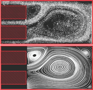
We present qualitative comparisons between numerical streamlines and PIV images of the corresponding experiments in figure 6 for the longer cavity length at two Reynolds numbers,  $Re = 7$ and
  $Re = 34$. When flow rate is low, the experiment shows the jet emerging symmetrically into the cavity. This pattern is shown in figure 6(a), where tracer particles indicate streamlines originating within the inflow channel. The numerical tricks described above and resulting in figure 5(c) did not produce an asymmetric solution at this lower Reynolds number.

Figure 6. A comparison of qualitative ‘for visualisation’ experiments with theoretical streamlines. All are for  $\alpha = 21.7$.
  $(a)$ Experiment (
 $Re = 7$).
  $(b)$ Numerics (
 $Re = 7$).
  $(c)$ Experiment (
 $Re = 34$).
  $(d)$ Numerics (
 $Re = 34$).
Figures 7(a,d) and 7(b,e) display velocity colour maps for the dimensionless numerical and experimental velocity fields for  $Re = 35$ and
  $\alpha = 8.3$ and
  $21.7$, respectively. (The driving pressure for the experiments in figure 6(a,d) was slightly different from the driving pressure for figure 7a–c resulting in the two different
  $Re$ values (
 $Re = 34$ and
  $Re = 35$, respectively).) These suggest the existence of a critical cavity length at which asymmetric solutions emerge. Although less relevant in a symmetry-breaking context, we have also compared experimental and theoretical velocity fields for the ‘offset-scope’ configuration (figure 1b) in figures 7(c) and 7(f), respectively. All three geometries in figure 7 demonstrate good visual agreement between PIV and simulation.

Figure 7. A comparison for (a–c) numerical simulations with (d–f) PIV experiments showing the velocity magnitude and vector directions. (a,d)  $\alpha = 8.3$, (b,e) and (c,f)
  $\alpha = 21.7$ (with far right the ‘offset-scope’ configuration). All are for
  $Re = 35$.
4.2. Bifurcation diagrams
We computed bifurcation diagrams as functions of  $Re$ and
  $\alpha$ using an implementation of numerical deflation techniques (Farrell et al. Reference Farrell, Birkisson and Funke2015) within Firedrake. Deflation is a technique for calculating multiple solutions of a nonlinear problem from a fixed initial guess. When a regular solution is found with Newton's method, a modified problem is constructed that retains all solutions of the base problem, except the one that has been found. Newton's method can then be applied from the same initial guess, and if it converges, it will converge to a distinct solution. The process can then be repeated until Newton's method fails to find any solutions.
To test the stability of the branches at representative points on the bifurcation diagram, we determine transient behaviour by using the computed steady-state solution (with an added random perturbation) as the initial condition to a time-dependent finite element solver for the incompressible Navier–Stokes equations. (We take  $\boldsymbol {u}(\boldsymbol {x}) + \boldsymbol {\epsilon }(\boldsymbol {x})$ as the initial condition, where
  $\boldsymbol {u}$ is the calculated steady-state solution and
  $\boldsymbol {\epsilon }$ is an independent normally distributed random variable with mean zero and standard deviation
  $0.01$, at each value of
  $\boldsymbol{x}$. If the transient solution moves away from the initial condition, the branch is marked unstable; otherwise it is stable. We terminate the solver once a steady-state has been reached – i.e. when the solver requires zero Newton iterations to update the solution from the previous time step.)
For expanding channels, the maximum value of the cross-stream velocity along the centreline ( $y = 0$) provides a good functional of the solution for visualising bifurcation phenomena, as this value will be zero for symmetric flows, and non-zero otherwise (Battaglia et al. Reference Battaglia, Tavener, Kulkarni and Merkle1997). However, due to our confined geometry, the cross-stream velocity along the centreline of the cavity may have two peaks of opposite sign; see, for example, figure 6(d). Thus, we define a bifurcation functional,
  $v_{{m}}$, to be the value of the first peak; that is, the one with smaller
  $x$-value coordinate. Denoting the cross-stream velocity along the centreline
  $v_{{c}} = v^{\star }(x,0)/U$,
  $v_{{m}}$ is hence defined as
 \begin{align} v_{{m}} = \begin{cases} \max(v_{{c}}), & \text{argmax}(v_{{c}}) < \text{argmin}(v_{{c}}),\\ \min(v_{{c}}), & \text{otherwise}. \end{cases} \end{align}
 In figure 8(a), we plot the computed bifurcation diagram for  $\alpha = 21.7$ as a function of Reynolds number – branch stability is indicated by solid lines (stable) and dashed lines (unstable) – as well as the relevant experimental data. We obtain a pitchfork in the numerical solutions, where the appearance of the asymmetric branches corresponds to loss of stability of the symmetric branch. Figure 8 demonstrates good quantitative agreement between numerics and experiments; however, for
  $Re < 24$, only one asymmetric jet direction was obtained experimentally, and we were unable to switch the direction of the flow via the experimental technique described in § 2.2. This indicates a disconnected pitchfork in the experimental results, as is often found, due to small imperfections in the experimental set-up (Fearn et al. Reference Fearn, Mullin and Cliffe1990; Hawa & Rusak Reference Hawa and Rusak2000; Mullin et al. Reference Mullin, Shipton and Tavener2002). To illustrate the effect of imperfections on the bifurcation diagram, in figure 8(b) we add a small asymmetry to the domain (we take the upper outflow to be
  $10\,\%$ smaller than the lower one), and compute the resulting bifurcation diagram, comparing this, again, with the experimental data. It is difficult to quantify the imperfections in the experimental set-up, but we see that an asymmetry in the computational domain can disconnect the bifurcation diagram in a manner that matches qualitatively with the experimental data. Additionally it is worth recalling when comparing bifurcation results between numerics and experiment, that flows in the physical experiments, although conducted in a geometry where the third dimension is nearly 25 times larger than the width of the inflow channel, will inherently be three-dimensional. The effect of the distance between the bounding walls in the third dimension on bifurcation phenomena in a sudden expansion channel was explored numerically by Guevel et al. (Reference Guevel, Allain, Girault and Cadou2018). The critical Reynolds number for the first primary steady bifurcation was shown to converge to the value for two-dimensional flow, albeit slowly, as the distance between the bounding walls in the third dimension was increased.

Figure 8. Black lines denote results of numerical simulations. Solid and dashed lines are solution branches conjectured to be stable and unstable, respectively. Panel  $(a)$ is a plot of
  $v_{{m}}$ as a function of Reynolds number. Data points from PIV experiments for
  $\alpha = 21.7$ are in red, with error bars providing the standard deviation. Panel
  $(b)$ adds a small asymmetry to the domain; here, the upper
  $b$ separation is
  $10\,\%$ smaller than the lower one. Panel
  $(c)$ shows the bifurcation structure as a function of
  $\alpha$ for fixed
  $Re = 35$. Data points are from the PIV experiments with red for
  $\alpha = 21.7$ and blue for
  $\alpha = 8.3$. Panel
  $(d)$ is a function of
  $Re$ for fixed
  $\alpha = 0.875\times 0.06^{-1} \approx 14.58$. The inset plot shows a zoomed-in view of the area encompassed by the yellow box (from
  $Re = 16.14$ to
  $Re = 21$). The grey and green dots denote a subcritical point and a supercritical point, respectively, which will collide to form a C
 $-$ coalescence point as
  $\alpha$ is increased.
  $(a)$
$(a)$ $\alpha = 21.7$;
  $(b)$
$(b)$ $21.7$;
  $(c)$
$(c)$ $Re = 35$; and
  $(d)$
$(d)$ $\alpha = 14.58$.
We also compute bifurcation diagrams as a function of  $\alpha$. An example is shown for fixed
  $Re = 35$ in figure 8(c), where we also plot experimental measurements for the two experimental cavity lengths at this Reynolds number. As predicted, for cavity lengths below a critical value (
 $\alpha \approx 14.5$), only the symmetric solution exists.
Interestingly, in the numerical solutions, we observe a hysteresis loop and a small range of  $\alpha$ for which both the symmetric and asymmetric branches may be stable. Now fixing
  $\alpha \approx 14.58$, we vary
  $Re$, to obtain the bifurcation diagram shown in figure 8(d). A similar hysteresis loop at low Reynolds number has been shown for flow in a symmetric channel with an expanded section, emerging at a particular aspect ratio and Reynolds number, termed a C+ coalescence point (Mullin et al. Reference Mullin, Shipton and Tavener2002). As the aspect ratio is increased, the subcritical point in the hysteresis loop (analogous to the green point in figure 8) moves and eventually coalesces with the supercritical point (in grey), colliding to form a C
 $-$ coalescence point. Although we have only computed slices through the bifurcation structure that exists in a three-dimensional space, and have not explicitly determined the trajectories of limit points, we postulate a similar behaviour for the bifurcation structure in our geometry as for the channel with an expanded section (Mullin et al. Reference Mullin, Shipton and Tavener2002). We also computed eight additional solution branches at
  $Re>100$ and
  $\alpha \approx 14.58$ (results not shown). This is not surprising given that a rich structure to solutions of the Navier–Stokes equations in a two-dimensional expansion channel at Reynolds numbers less than a few hundred is well established (Alleborn et al. Reference Alleborn, Nandakumar, Raszillier and Durst1997).
The results in this section highlight that even for the simplest symmetric representative geometry, complex asymmetric flow patterns arise. In the following section, we consider how the structure of the flow affects the time required for a passive tracer (representing debris within the kidney) to exit the cavity.
5. The effect of flow structure on tracer transport
We consider a passive tracer in a steady velocity field, the latter computed as a solution to (3.8) with boundary conditions (3.9). We assume an initial concentration in the cavity (sufficiently low such that the tracer does not affect the flow) that is subsequently transported through the fluid by advection and diffusion.
5.1. Theoretical formulation
We consider the tracer concentration  $c^{\star }(\boldsymbol {x}^{\star },t^{\star })$ to diffuse with coefficient,
  $\mathcal {D}$, and to be passively advected by the flow of fluid within the cavity (figure 1a). Conservation of mass provides
 \begin{equation} \frac{\partial c^{\star}}{\partial t^{\star}} + \nabla^{\star}\boldsymbol{\cdot}\boldsymbol{J}^{\star} = 0, \qquad \boldsymbol{J}^{\star} = -\mathcal{D}\nabla^{\star}c^{\star} + \boldsymbol{u}^{\star}c^{\star}, \end{equation}
where stars denote dimensional quantities and  $\boldsymbol {u}^{\star }$ is determined a priori by solving (3.8) with boundary conditions (3.9a–e). We note that due to the incompressibility of the fluid, (5.1) is equivalent to
 \begin{equation} \frac{\partial c^{\star}}{\partial t^{\star}} = \mathcal{D}\boldsymbol{\nabla}^{{\star}2} c^{\star} - \boldsymbol{u}^{\star}\boldsymbol{\cdot}\nabla^{\star} c^{\star}. \end{equation}
We impose no movement of the tracer through the inflow or solid walls and no diffusion through the outflows
 \begin{gather} \boldsymbol{J}^{\star}\boldsymbol{\cdot}\boldsymbol{n} = 0, \quad\text{on }\varGamma^{\star}_{{in}},\varGamma^{\star}_{{{wall}}}, \end{gather}
 \begin{gather} \nabla^{\star}c^{\star}\boldsymbol{\cdot}\boldsymbol{n} = 0, \quad\text{on }\varGamma^{\star}_{{{out}}}, \end{gather}
where  $\boldsymbol {n}$ is the unit vector normal to each boundary. We assume an initial tracer concentration of density
  $C$ that is uniform in a circle of radius
  $c_r^{\star }$, centred at
  $\boldsymbol {x}^{\star }_c = (x^{\star }_c,y^{\star }_c)$, which we approximate by
 \begin{equation} c^{\star}(\boldsymbol{x}^{\star},0) = \frac{C}{2}\left[1 + \tanh\left(\frac{d^{\star}(\boldsymbol{x}^{\star})}{\delta^{\star}}\right)\right], \end{equation}
where  $\delta ^{\star }$ controls the width of the step function approximation and
 \begin{equation} d^{\star}(x^{\star},y^{\star}) = c^{\star}_r - \sqrt{(x^{\star}-x^{\star}_c)^2 + (y^{\star}-y^{\star}_c)^2} \end{equation}
ensures an initially circular distribution.
We non-dimensionalise as follows
 \begin{equation} c = \frac{c^{\star}}{C}, \quad t = \frac{Ut^{\star}}{a}, \quad \boldsymbol{u} = \left(\frac{u^{\star}}{U},\frac{\alpha v^{\star}}{U}\right), \quad \boldsymbol{x} = \left(\frac{x^{\star}}{\alpha a}, \frac{y^{\star}}{a}\right), \end{equation}
where time has been non-dimensionalised using the advective time scale. Thus, (5.2) becomes
 \begin{equation} \frac{\partial c}{\partial t} = \frac{1}{Pe}\left(\frac{1}{\alpha^2}\frac{\partial^2c}{\partial x^2} - \frac{\partial^2c}{\partial y^2}\right) - \frac{1}{\alpha}\left(u\frac{\partial c}{\partial x} + v\frac{\partial c}{\partial y}\right), \end{equation}
where the Péclet number
 \begin{equation} Pe = Ua/\mathcal{D}, \end{equation}
characterises the relative influence of advection with respect to diffusion.
The dimensionless, scaled, initial condition (5.4), (5.5) is
 \begin{equation} c(x,y,0) = \frac{1}{2}\left[1 + \tanh\left(\frac{\textrm{d}(\boldsymbol{x})}{\delta}\right)\right], \end{equation}
where
 \begin{equation} \textrm{d}(x,y) = c_r-\sqrt{\alpha^2(x-x_c)^2+(y-y_c)^2}, \end{equation}
and
 \begin{equation} x_c = \frac{x_c^{\star}}{\alpha a}, \quad y_c = \frac{y_c^{\star}}{a}, \quad c_r = \frac{c_r^{\star}}{a}, \quad \delta = \frac{\delta^{\star}}{a}. \end{equation}
Boundary conditions (5.3) are
 \begin{gather} \boldsymbol{J}\boldsymbol{\cdot}\boldsymbol{n} = 0, \quad\text{on }\varGamma_{{in}},\varGamma_{{{wall}}}, \end{gather}
 \begin{gather} \boldsymbol{\nabla} c\boldsymbol{\cdot}\boldsymbol{n} = 0, \quad\text{on }\varGamma_{{{out}}}, \end{gather}
where  $\boldsymbol {J} = -(1/Pe)\boldsymbol {\nabla } c + \boldsymbol {u}c$ and
  $\boldsymbol {\nabla } = (\alpha ^{-1}\partial /\partial x, \partial /\partial y)$.
To quantify the rate at which the passive tracer exits the cavity we define the percentage loss at time  $t$ as
 \begin{equation} \% \text{ loss} = \frac{\iint_{\varOmega}\left[ c(x,y,0)-c(x,y,t)\right]\,\mathrm{d}{\varOmega}}{\iint_{\varOmega} c(x,y,0)\,\mathrm{d}{\varOmega}}. \end{equation}
We define a ‘washout time’ metric,  $T_{90}$ corresponding to the time required for
  $90\,\%$ of the tracer to exit the cavity, i.e.
 \begin{equation} \frac{\iint_{\varOmega}\left[ c(x,y,0)-c(x,y,T_{90})\right]\,\mathrm{d}{\varOmega}}{\iint_{\varOmega} c(x,y,0)\,\mathrm{d}{\varOmega}} = 0.9, \end{equation}
where the initial concentration is set by (5.9), (5.10). We note that as concentration only advects through the cavity outlets by (5.12b),  $T_{90}$ can also be defined by
 \begin{equation} \frac{\int_0^{T_{90}}\left[\int_{\varGamma_{{out}}}c\boldsymbol{u}\boldsymbol{\cdot}\boldsymbol{n}\,\mathrm{d}{y}\right]\,\mathrm{d}{t}}{\iint_{\varOmega}c(x^{\star},y,0)\,\mathrm{d}{\varOmega}} = 0.9. \end{equation}
We have verified that both formulas agree, and use the former as it only requires spatial integration and is thus less prone to accumulation of numerical error over time.
5.2. Numerical details
We approximated the concentration function with piecewise linear elements on the same mesh as the velocity field (see § 3.1). The velocity field was solved for using the methods in § 3.1 and subsequently restored to drive the advective term in (5.7). Equation (5.7) was discretised in time using a Crank–Nicolson scheme, and we added a mesh-dependent Streamline-Upwind Petrov-Galerkin (known as SUPG) stabilisation term, as described in Franca, Frey & Hughes (Reference Franca, Frey and Hughes1992) as standard Galerkin discretisations of advection–diffusion equations are oscillatory in the advection-dominated regime (Silvester, Elman & Wathen Reference Silvester, Elman and Wathen2014). We validated our code using the method of manufactured solutions, with details presented in appendix B.2.
5.3. Effect of flow pattern
In § 4.1, we determined the existence of multiple flow solutions in a symmetric domain, and additionally, computed flow patterns corresponding to both centred and offset inlets. In this section, we initially place the debris cloud in the centre of the cavity, and consider the effect of different flow patterns on the washout time. In figure 9, we plot (5.13) as a function of time, for three different advecting flow patterns: symmetric, asymmetric and offset. All are at  $Re = 34$, cavity length corresponding to
  $\alpha = 21.7$ and
  $Pe = 10^3$. The washout times
  $T_{90}$ are indicated by the colour bar to the right of the streamline figures, corresponding to the colours of the circular dust clouds in figures 9(a–c), and the lines in figure 9(d). The symmetric flow pattern provides the shortest washout time, and the offset one the longest. Placing the tracer initially in the centre for the symmetric flow profile allows it to be immediately transported along streamlines that advect out of the cavity, with only trace amounts of debris entering the two vortices (figure 9a). In contrast, both the asymmetric and offset flow patterns contain vortices of closed streamlines surrounding the initial concentration, resulting in longer washout times in an advection dominated regime (
 $Pe = 10^3$). To further explore the possibility of vortical streamlines trapping debris and causing longer washout times, we examine the effect of the initial position of a tracer within the flow pattern in figure 9(b), as well as the Péclet number, in the following sections.

Figure 9. The percentage loss for  $Pe = 10^3$ as a function of time for three different flow patterns. The corresponding patterns are shown in (a–c), with the colour of the initial concentration indicating the value of
  $T_{90}$.
  $(a)$ Symmetric.
  $(b)$ Asymmetric.
  $(c)$ Offset. (d)
  $Re = 34$,
  $\alpha = 21.7$.
5.4. Effect of tracer position
To investigate how the initial position of the debris cloud  $\boldsymbol {x}_c$, affects
  $T_{90}$, we consider five equally spaced positions within the cavity, which we label
  $A$,
$A$,  $B$,
$B$,  $C$,
$C$,  $D$ and
  $E$, as indicated in figure 10. The colours of the tracers in figure 10 demonstrate the corresponding washout times, (5.14). Results are shown for three different values of
  $Pe$ –
  $10^3, 10^2$ and
  $10^1$ – in figures 10(a), 10(b) and 10(c), respectively. Initial placement of the tracer in positions of vortical flow (
 $A$,
$A$,  $B$ and
  $C$) results in larger washout times than initial placement in streamlines that advect directly out of the cavity (
 $D$,
$D$,  $E$). This difference is more pronounced for larger values of
  $Pe$. As we decrease
  $Pe$ (analogous to increasing the diffusion coefficient as we have scaled on the advective time scale), diffusion out of areas with closed streamlines is faster, and total washout time decreases for positions
  $A$,
$A$,  $B$ and
  $C$. Interestingly, an increase in diffusion is not always advantageous in decreasing washout –
  $E$ has a slower washout time for
  $Pe = 10^1$ than
  $Pe = 10^2$, as the tracer is initially on streamlines that advect directly out of the cavity, so diffusion away from these streamlines is counterproductive to washout.

Figure 10. Value of  $T_{90}$ for five values of
  $\boldsymbol {x}_c$. Panels
  $(a)$,
  $(b)$ and
  $(c)$ are for
  $Pe = 10^3$,
  $10^2$ and
  $Pe = 10^1$, respectively.
5.5. Effect of  $Pe$
$Pe$

Based on the work of Rhines & Young (Reference Rhines and Young1983), we propose that for tracer that initially resides in a vortex, the clearance time is potentially influenced by any (or all) of the following three dimensional time scales:
 \begin{equation} T_{a}^{\star} \sim (\ell_{\mathcal{D}}/U)Pe^{1/3}, \quad T_{b}^{\star} \sim \left(\ell_{\mathcal{D}}^2/(Ua)\right)Pe, \quad T_{c}^{\star} \sim \ell_{U}/U, \end{equation}
where  $\ell _{\mathcal {D}}$ is the diffusive distance required (i.e. vortex size for initial positions
  $A$,
$A$,  $B$ and
  $C$), and
  $\ell _{U}$ the advective distance (i.e. the distance of the vortex centre from an outlet);
  $T^{\star }_a$ is the time required for the tracer to distribute uniformly throughout the vortex and reach the dividing streamline,
  $T^{\star }_b$ is the time to escape the closed streamlines via diffusion and
  $T^{\star }_c$ is the time to advect from the vortex to an outlet. Scaling equations (5.16) by the advective time-scale as in (5.6b) we obtain the dimensionless forms
 \begin{equation} T_{a} \sim (\ell_{\mathcal{D}}/a)Pe^{1/3}, \quad T_{b} \sim (\ell_{\mathcal{D}}/a)^2Pe, \quad T_{c} \sim \ell_{U}/a. \end{equation}
We note that, as we have scaled on the advective time,  $T^{\star }_c$ is independent of
  $Pe$. Hence, the total washout time for dust that initiates within a vortex is the sum of the three components (5.17)
 \begin{equation} T \sim T_a + T_b + T_c = (\ell_{\mathcal{D}}/a)Pe^{1/3} + (\ell_{\mathcal{D}}/a)^2Pe + \ell_U/a. \end{equation}
 In figure 11 we plot  $T_{90}$ as a function of
  $Pe$ for concentration initiating at positions
  $A$,
$A$,  $B$,
$B$,  $C$,
$C$,  $D$ and
  $E$ (figure 10). For positions
  $D$ and
  $E$ which are not in vortices,
  $\ell _{\mathcal {D}} = 0$, and hence for large
  $Pe$, where diffusion is negligible, we will expect
  $T_{90}$ to scale with
  $T_c$, which is independent of
  $Pe$, according to (5.17c). This is seen by the flat grey and black lines as we increase
  $Pe$ in figure 11. For concentration that is initially in a vortex (positions
  $A$,
$A$,  $B$ and
  $C$) we see the competing effects of
  $T_a$,
  $T_b$ and
  $T_c$. For moderate
  $Pe$ and small vortices where
  $\ell _{\mathcal {D}}/a < 1$,
  $T_a$ may dominate over
  $T_b$, and this is seen by the initial
  $Pe^{1/3}$ scaling for positions
  $A$ and
  $B$. For
  $\ell _{\mathcal {D}}/a > 1$, however,
  $T_b$ will quickly dominate as
  $Pe$ increases; hence we see a linear slope emerging for position
  $C$. For the
  $Pe$ range considered, this is not seen for positions
  $A$ and
  $B$, where the vortices are small, and hence a delicate balance exists between
  $T_a$,
  $T_b$ and
  $T_c$. However, from (5.18), we expect
  $T_{90} \propto Pe$ as
  $Pe\rightarrow \infty$. We also note a decrease in
  $T_{90}$ with diffusion for positions
  $A$,
$A$,  $D$ and
  $E$ with
  $Pe$ when
  $Pe$ is approximately
  $10^1\leq Pe\leq 10^2$. Here, diffusion takes concentration on to the closed streamlines in the centre of the cavity, where it will require more time to escape. (As tracer originating at position
  $A$ is already in a region of closed streamlines, diffusion allows some tracer to escape via the top of the vortex and advect through the proximal outflow. However, a significant proportion of the tracer still diffuses to the large central vortex, explaining the initial decrease in
  $T_{90}$ in figure 11.) Thus, the existence of multiple vortices which the tracer can move between complicates the approximation of
  $T_{90}$ beyond a simple expression such as (5.18).

Figure 11. A log–log plot of  $T_{90}$ as a function of
  $Pe$ for dust placed in positions
  $A$,
$A$,  $B$,
$B$,  $C$,
$C$,  $D$ and
  $E$. Points at
  $Pe = 10^1, 10^2$ and
  $10^3$, correspond to the snapshots in figure 10. Péclet numbers considered:
  $Pe = 10^x$ for
  $200$ evenly distributed
  $x$ values
  $x \in [1,3]$.
5.6. Effect of instantaneous flow switch
The results in figures 10 and 11 demonstrate that remaining within a steady vortex can induce extremely large times required for the passive tracer to exit the cavity. We hypothesise that disrupting the flow pattern may increase mixing of the tracer and improve washout times. Motivated by the experiment in figure 3, where we saw mirror asymmetric flows could be established, with the opportunity to switch between them by blocking and re-opening an outflow, we instantaneously switch  $\boldsymbol {u}$ in (5.7) from one mirror branch to the other at a time
  $s$ (see figure 12a,b). We recognise that a fully transient computation is more appropriate, but this approach provided rapid insights. We denote the washout time resulting from a switch at time
  $s$ by
  $T^{s}_{90}$. Figure 12(c) shows the change in
  $T^{s}_{90}$ from
  $T_{90}$ (when no ‘flow switching’ is imposed) as a function of
  $s/T_{90}$ for concentration initially placed in the centre of the cavity (position
  $C$ in figure 10) and
  $Pe = 10^2$. We see that instantaneously switching from figures 12(a) to 12(b) at time
  $t = s$, when
  $s <0.93T_{90}$ results in a decreased washout time,
  $T^s_{90}$. The oscillations in figure 12(c) occur when switching during the phase where the tracer concentration is averaging throughout the vortex,
  $T_a$ (5.17). During this initial period, as position
  $C$ does not align precisely with the centre of the vortex, the tracer swirls along the streamlines. Switching from figures 12(a) to 12(b) when the tracer is above the centreline of the vortex (for example at the position indicated in green in figure 12a) moves the tracer further towards the outside of the vortex. This is beneficial both because the tracer is closer to streamlines that advect directly out of the cavity and because the velocity is faster, thereby increasing shear-enhanced diffusion of the tracer. Switching once the tracer has distributed uniformly throughout the vortex, i.e.
  $s > T_a$, still moves some of the tracer on to the advective streamlines (as the vortex is not central within the cavity), but as the position of the tracer is relatively constant, we see a dampening of the oscillations in figure 12(c). Although not shown, for higher values of
  $Re$ the vortex is less central within the cavity, and hence switching flow branches can move the tracer onto a streamline that advects directly out of the cavity, thus inducing further reductions in washout time. We caution, however, that switching the flow once the tracer has diffused out of the vortex can actually increase washout times. This is seen in figure 12(c), where, when
  $s/T_{90} \rightarrow 1$,
  $T^s_{90}-T_{90}>0$. This is similar to the effect seen in figure 10, where an increase in diffusion caused an increase in washout time for tracer
  $E$, which is initially placed on streamlines that advect out of the cavity. Once the tracer has reached open streamlines that leave the cavity, switching the advecting flow pattern may move tracer back onto closed streamlines, slowing washout times. This ‘flow-switching’ experiment draws parallels with the blinking vortex model, a classic example of chaotic mixing (Aref Reference Aref1984).

Figure 12. Panel  $(a)$ shows the velocity field for
  $t<s$, and
  $(b)$ for
  $t\geq s$. Panel
  $(c)$ is the decrease in washout time as a function of switch time with
  $Pe = 10^2$. The green and red circles in
  $(a)$ illustrate approximate position of the tracer bulk when ‘flow switching’ corresponds to peaks and troughs in
  $(c)$, respectively.
6. Summary and discussion
Irrigation fluid is driven into the renal pelvis during ureteroscopy to wash out kidney stone debris. We investigated the fluid mechanics of this process in a simplified, rectangular geometry and considered how flow patterns affect the time required for successful clearance of the debris.
We began by studying symmetry breaking in the considered geometry, which we determined occurs as a function both of Reynolds number and the aspect ratio of the cavity. We adopted a complementary approach, performing both numerical simulations and particle image velocimetry experiments, and obtained excellent qualitative and quantitative agreement. We computed bifurcation diagrams as functions both of cavity aspect ratio and the Reynolds number of the flow via numerical deflation techniques. A rich bifurcation structure was observed including hysteresis loops for a small range of cavity lengths and Reynolds numbers. The PIV experiments demonstrated the presence of a disconnected pitchfork bifurcation as a function of Reynolds number for fixed aspect ratio. We determined both critical Reynolds numbers and aspect ratios for the existence of asymmetric flow patterns.
For a particular Reynolds number and cavity length, we studied the effect of initial placement of a passive tracer within the flow field on the time required for  $90\,\%$ of the concentration to advect out of the cavity (the washout time) by coupling the computed velocity field to an advection–diffusion equation. We calculated results for a variety of Péclet numbers, and found that when the tracer is initially placed in a vortex, the washout time (scaled by the advective time-scale) is comprised of three contributions: first, a time for the tracer to distribute uniformly throughout the vortex via mechanisms of shear-enhanced diffusion which scales with
  $Pe^{1/3}$; second, a time for the tracer to escape the closed streamlines requiring the full diffusion time which scales with
  $Pe$; third, a time for the tracer to advect from the vortex to a cavity outlet, which depends primarily on the advecting velocity and is hence nearly independent of
  $Pe$ (if
  $Pe$ is low, however, effects of diffusion may dominate and move the tracer away from the advective streamlines). The dominant scaling depends on the initial position of the tracer in relation to vortices within the cavity and streamlines that advect out of the cavity.
Finally, we considered the effect of switching from one asymmetric solution to its mirror pair on the advection and diffusion of the passive tracer, and found that this often results in a reduction in washout time from the ‘no-switching’ case.
Our study was motivated by the washout of kidney stone debris in ureteroscopy procedures. Here, it is worth highlighting the simplifying assumptions and potential next steps in bringing this work closer to clinical translation. First, our idealised set-up is obviously different from the renal geometry both in the rectangular shape and in our restriction to two dimensions. Hence one important extension to the work presented here will be to consider the effect of the third dimension on flow patterns and resulting washout times. Although solving the steady Navier–Stokes equations in a two-dimensional rectangular domain allowed exploration of fundamental principles – such as the existence of multiple solutions, and the effect of vortical flow on the clearance of debris that is passively advected with the addition of weak diffusion – three-dimensional effects will realistically play a significant role. Additionally, we chose a geometry with perfectly sharp corners which do not exist in the true geometries of the ureteroscope and renal pelvis. The shape of the domain boundary has a quantitative effect on flow separation and recirculation, and thus performing experiments and simulations in more realistic three-dimensional geometries is a critical next step in our study of ureteroscopy irrigation.
It is important to recall that we have assumed flow to be steady throughout this article. It would also be interesting to see how transience affects our results, particularly in § 5.6, where we investigated the effect of an instantaneous switch in the direction of the flow on washout time. The instantaneous switch is an approximation of the experiment in figure 3 (and the supplementary movie), where transient behaviour, as the flow moves between two stable states, is clearly visible.
Another critical component of the realistic renal pelvis during ureteroscopy irrigation, currently missing from our analysis, is the presence of a solid obstruction – a kidney stone – that will disrupt the flow patterns. Thermal energy delivered via a thin, optical fibre continuously degrades the stone, and while very fine dust may be modelled effectively by considering advection with the irrigation fluid and passive diffusion, (5.1), the dynamical motion of larger fragments will be intricately coupled to the fluid behaviour. Modelling all facets of this system – the continual deterioration of the kidney stone, along with the fluid–structure interaction of stone particles and the fluid – is highly complex, but must be considered for a full understanding of the interplay between saline delivery and efficient kidney stone removal.
The points above underscore the significant work needed to bring our analysis to the level of quantitative predictions for ureteroscopy. Nevertheless, our model provides a first qualitative step in understanding the potential impact of vortical structures on dust washout. Indeed, the orders of magnitude difference in washout times that we observe suggests that procedural steps to disrupt vortices may have significant impact on reducing procedure times. Moreover, increasing irrigation flow rate is typically considered synonymous with improved visualisation; however, our results indicate that, depending on the diffusive properties of kidney stone debris, increasing flux may not be the most efficient method through which to improve clearance. Extrapolating the results of our study in a simple two-dimensional cavity, we hypothesise that debris within the working space during ureteroscopy may get trapped in vortices, resulting in large washout times. Disturbing the flow when debris is trapped in vortices can move debris away from the vortex centre, onto faster streamlines which allow debris to advect out of the cavity, resulting in shorter times required to clear the field of view.
Acknowledgements
This publication is based on work supported (or partially supported) by the EPSRC Centre For Doctoral Training in Industrially Focused Mathematical Modelling (EP/L015803/1) in collaboration with Boston Scientific. S.L.W. and A.A.C-P. are grateful to the Royal Society for funding in the form of a Leverhulme Trust Senior Research Fellowship and a University Research Fellowship, respectively. P.E.F. was supported by EPSRC grants EP/R029423/1 and EP/V001493/1. The authors would like to acknowledge the support of Boston Scientific Corporation. The authors are also grateful for discussions with M. Heil on numerical detection of symmetry breaking, along with valuable input from F. Wechsung on implementing the Navier–Stokes solver. The authors would also like to acknowledge several insightful conversations with T. Mullin on symmetry breaking in fluid flows.
Declaration of interests
The authors report no conflict of interest.
Supplementary movie
Supplementary movie is available at https://doi.org/10.1017/jfm.2020.583.
Appendix A. Outflows
In this paper, we solve (3.8) in the light-pink domain in figure 1(a), prescribing zero-stress boundary conditions, (3.9c,d), on  $\varGamma _{{out}}$, a Poiseuille profile on
  $\varGamma _{{in}}$, (3.9a,b), and no slip on
  $\varGamma_{wall}$, (3.9e).
Here, we validate truncating the numerical domain to include only the cavity, and not the outflow channels present in the particle image velocimetry experiments (§ 2), by simulating flow on the domain pictured in figure 13, with outflow channels of dimensional length 24 cm (see figure 2a), denoted  $l_{{out}}$ when non-dimensionalised with respect to
  $a = 0.06\ \textrm {cm}$. As we scaled the horizontal coordinate by
  $\alpha$ and solve the scaled (3.8), we build a mesh with outflow channels of length
  $l_{{out}}/\alpha$. As outflow conditions we prescribe zero normal stress and parallel outflow
 \begin{equation} 2u_x - p =0, \quad v = 0, \quad \text{on }\varGamma_{out}, \end{equation}
and as before, a Poiseuille inlet profile, (3.9a,b), and no slip on the walls, (3.9e).

Figure 13. The considered numerical domain including outflow channels.
We plot the bifurcation diagram for  $\alpha = 21.7$,
  $Re\in [0,40]$, in figure 14 (black marks) including points for the simulations at the same parameters in the domain with outflow channels with conditions (A 1) (grey marks). We see the bifurcation structure remains unchanged, with only small discrepancies between the numerical results.

Figure 14. A plot of  $v_{{m}}$ as a function of Reynolds number, comparing the results in figure 8(a) (black marks) with those including outflows (grey marks).
Appendix B. Numerical convergence
B.1. Navier–Stokes computations
To demonstrate the effect of mesh size on the numerical solutions to the Navier–Stokes equations, in figure 15 we compute the bifurcation diagram for  $\alpha = 21.7$ using
  $2.1\times 10^4$ elements (black points) and
  $8.4\times 10^4$ elements (red points). As the two sets of points are nearly indistinguishable, we present a zoomed-in view between
  $Re = [36.5,37.5]$ and
  $v_{{m}} = [0.2555, 0.2562]$ in the yellow box in figure 15; this inset plot demonstrates the difference between
  $v_{{m}}$ values calculated with the different mesh sizes is typically
  $O(10^{-3})$. Furthermore, the error in the velocity field arising due to mesh size is demonstrably smaller than the error arising due to the truncation of the flow domain.

Figure 15. A plot of  $v_{{m}}$ as a function of Reynolds number for
  $\alpha = 21.7$, calculated using
  $2.1\times 10^4$ elements (black points) and
  $8.4\times 10^4$ elements (red points). A zoomed-in view around
  $Re = [36.5,37.5]$,
  $v_{{m}} = [0.2555, 0.2562]$ is shown in the yellow box.
B.2. Advection–diffusion computations
To test the code used to solve (5.7) we used the method of manufactured solutions. We chose as exact solution the time- and space-dependent function
 \begin{equation} c_{{ex}}(x,y,t) = [(x-x_0)^2 + (y-y_0)^2]\cos(t), \end{equation}
where  $(x_0,y_0) = (1/0.12,0)$ was taken to be the centre of the rectangular domain. We then solved
 \begin{equation} \frac{\partial c_{{num}}}{\partial t} = \frac{1}{Pe}\left(\frac{1}{\alpha^2}\frac{\partial^2c_{{num}}}{\partial x^2} - \frac{\partial^2c_{{num}}}{\partial y^2}\right) - \frac{1}{\alpha}\left(u\frac{\partial c_{{num}}}{\partial x} + v\frac{\partial c_{{num}}}{\partial y}\right) + f(x,y,t) \end{equation}
using the methods described in § 3.1, where
 \begin{equation} f(x,y,t) = \frac{\partial c_{{ex}}}{\partial t} -\frac{1}{Pe}\left(\frac{1}{\alpha^2}\frac{\partial^2c_{{ex}}}{\partial x^2} - \frac{\partial^2c_{{ex}}}{\partial y^2}\right) - \frac{1}{\alpha}\left(u\frac{\partial c_{{ex}}}{\partial x} + v\frac{\partial c_{{ex}}}{\partial y}\right). \end{equation}
We define the error to be
 \begin{equation} \|c_{{ex}}(t=5)-c_{{num}}(t=5)\|_{L^2} = \left[\iint_{\varOmega}\left(c_{{ex}}(x,y,5)-c_{{num}}(x,y,5)\right)^2\,\mathrm{d}{\varOmega}\right]^{1/2}. \end{equation}
In figure 16 we plot the error, (B 4), as a function of numerical time step  $\Delta t$. We fix the spatial step
  $\Delta x = \Delta t/2$, where
  $\Delta x$ is the distance between neighbouring points along the structured mesh. In figure 16 we observe the anticipated error reduction scaling with
  $\Delta t^2$. We chose the physical parameters from figure 10(b);
  $Re = 34$ for the velocity field, length scaling factor
  $\alpha = 1.3$, and Péclet number
  $Pe = 100$.

Figure 16. The error between the numerical solution and the manufactured solution for four different time steps. At each time step,  $\Delta x = \Delta t/2$; i.e. space and time are refined simultaneously.


