


1. Introduction
1.1. General context
Bubbles belong to the fascinating topics in fluid mechanics. They exhibit a variety of behaviours which have been intensively studied by engineers and scientists over the past decades. The reason for this interest is that bubbles are present in many environmental and industrial processes (waste water treatment, chemical reactors, river aeration, thermohydraulics…), the modelling and prediction of which requires a deep knowledge of the bubble physics. Among issues, it is fundamental to understand how bubbles rise (Clift, Grace & Weber Reference Clift, Grace and Weber1978; Magnaudet & Eames Reference Magnaudet and Eames2000), distribute in the flow (Serizawa, Kataoka & Michiyoshi Reference Serizawa, Kataoka and Michiyoshi1975; Mudde Reference Mudde2005; Balachandar & Eaton Reference Balachandar and Eaton2010), interact together and with the liquid around (Risso Reference Risso2018), deform (Clift et al. Reference Clift, Grace and Weber1978; Risso Reference Risso2000), grow/condense (Prosperetti Reference Prosperetti2017) or evolve in size through break-up and coalescence (Risso Reference Risso2000). All these aspects of bubble behaviour influence the transfers (momentum, heat and mass) at the gas–liquid interface (Risso Reference Risso2018) and doing so, are worthwhile to investigate. One important factor for bubbles is the degree of ‘cleanliness’ of the interface. Indeed, besides the heat and mass transfers with the bulk, the presence of surfactant or impurities at the surface can modify the forces acting on the bubble in a spectacular way (Clift et al. Reference Clift, Grace and Weber1978; Tagaki & Matsumoto Reference Tagaki and Matsumoto2011). It can, for instance, increase the drag force, hence reducing the bubble rising velocity, and modify the lift force that bubbles experience in shear flows, which influences their lateral motion in such flows.
1.2. Context of the study
This paper focuses on bubbles released inside a horizontal high-speed solid-body rotating flow. This flow situation is interesting because it can help us to understand how bubbles behave when they meet flow regions with locally high vorticity. These high vorticity regions are present in numerous flow situations such as (Green Reference Green1995) mixing layers, turbulence, recirculating flows and body wakes. They are characterized by the existence of low pressure minima at their centre. In many cases, studies showed that bubbles approaching these high vorticity regions are deflected towards the vortex core and trapped inside the region of minimum pressure. This typical behaviour was, for instance, reported by Sridhar & Katz (Reference Sridhar and Katz1995) with microscopic bubbles entrained in a vortex ring, by Jah & Govardhan (Reference Jah and Govardhan2015) with millimetric bubbles interacting with vortex rings, with cavitating bubbles in the tip vortices of propellers (see chapter XVIII by Chahine in Green Reference Green1995; Choi & Chahine Reference Choi and Chahine2003) and very recently by Cabut et al. (Reference Cabut, Michard, Simoens, Méès, Todoroff, Hermange and Le Chenadec2021) with air bubbles trapped in a counter-rotating vortex inside tire groves of a rolling car. Perhaps one of the most amazing examples of bubbles trapped by vortices is that given by videos of captive dolphins at play (Marten et al. Reference Marten, Shariff, Psarakos and White1996).
In all these situations the question is to know why and how the bubbles move towards the centre of the vortex and are trapped. Answering this question requires us to identify the forces acting on the bubbles in these situations. The seminal experiment of Naciri (Reference Naciri1992) showed that the horizontal solid-body rotating flow is rather representative of vortex regions and was adapted to measure some of these forces. He found that bubbles released in this type of flow experience, as in shear flows (Saffman Reference Saffman1965; Auton Reference Auton1987; Kariyasaki Reference Kariyasaki1987; Ervin & Tryggvason Reference Ervin and Tryggvason1997; Magnaudet & Legendre Reference Magnaudet and Legendre1998; Tomiyama et al. Reference Tomiyama, Tamai, Zun and Hosokawa2002; Takemura, Magnaudet & Dimitrakopoulos Reference Takemura, Magnaudet and Dimitrakopoulos2009; Hayashi, Legendre & Tomiyama Reference Hayashi, Legendre and Tomiyama2020), a lift force that, added to the other radial forces (pressure and added mass), make them spiral towards an equilibrium position located more or less close to the rotation axis, according to the rotation speed. The coordinates of this equilibrium position were used to measure the drag and lift coefficients.
Since that experiment, the behaviour of bubbles or solid particles in a horizontal solid-body rotation flow has been the object of several studies. Most of these studies address the determination of the drag and lift coefficients, either numerically (Bluemink et al. Reference Bluemink, Lohse, Prosperetti and Van Wijngaarden2008, Reference Bluemink, Lohse, Prosperetti and Van Wijngaarden2010) or experimentally from the equilibrium position (van Nierop et al. Reference van Nierop, Luther, Bluemink, Magnaudet, Prosperetti and Lohse2007; Rastello et al. Reference Rastello, Marié, Grosjean and Lance2009; Bluemink et al. Reference Bluemink, Lohse, Prosperetti and Van Wijngaarden2010; Rastello, Marié & Lance Reference Rastello, Marié and Lance2011, Reference Rastello, Marié and Lance2017). They are often limited to moderate rotation speeds, which avoids the bubble coming too close to the rotation axis and thus disturbing the solid-body rotating flow. Different situations were investigated, the case where the interface is clean (silicone oils, Rastello et al. Reference Rastello, Marié and Lance2011) and the case where the interface is partially or fully covered by impurities (water, Rastello et al. Reference Rastello, Marié, Grosjean and Lance2009, Reference Rastello, Marié and Lance2017). When the surface is contaminated and only in that case, it was shown to rotate with characteristics that are very similar to those of solid spheres immersed in that kind of flow (Bluemink et al. Reference Bluemink, Lohse, Prosperetti and Van Wijngaarden2008, Reference Bluemink, Lohse, Prosperetti and Van Wijngaarden2010). This results in an extra ‘Magnus’-like lift force and a separated wake behind the bubble, whose separation angle (the angle from the bubble rear at which the wake detaches from the bubble) is higher than that observed at the same Reynolds number on a solid non-rotating sphere in a uniform flow (Johnson & Patel Reference Johnson and Patel1999). Details on this separated wake were recently reported in Rastello & Marié (Reference Rastello and Marié2020).
1.3. Objectives
The novelty of this study compared with previous ones lies in the high rotation speeds which are explored. In this case, the bubble stabilizes close to the rotation axis, thus mimicking the bubbles trapped in a vortex core. This problem was analytically formulated by Rosenthal (Reference Rosenthal1962), the effect of gravity being neglected. The bubble, that is assumed spherical at zero rotation velocity, is shown to stretch, with its length increasing along the rotation axis as the rotation speed increases. The author derives a mathematical expression, providing the bubble elongation as a function of the rotation speed, for a given bubble volume. He also performs a stability analysis of these bubbles subjected to small sinusoidal disturbances, and shows that, within the axisymmetric assumption considered, increasing the rotation speed stabilizes the bubble.
Our first objective in the present study is to check experimentally if bubbles still behave in a comparable way when buoyancy breaks the symmetry of the problem. Practically, we inject bubbles of various given volumes into a cell rotating along a horizontal axis, and study their mean shape and aspect ratio as a function of the rotation speed. We can also determine the forces acting on the bubble from the bubble equilibrium position. Our second objective is then to measure the mean drag and lift forces acting on the bubble for these strongly inertial conditions.
We describe the experimental set-up and associated techniques in § 2. After a brief dimensional analysis of the problem, we discuss in § 3 the variations of the bubble aspect ratio as a function of relevant dimensional groupings. We next discuss in § 4 the question of the mean position of the bubble, and the related issue of the lift and drag forces acting on the bubble.
2. Experiment
2.1. Experimental set-up
The experimental apparatus is shown in figure 1. A cylindrical Plexiglas tank of diameter 11 cm and length 10 cm is rotated around its horizontal axis  $z$. The tank is fixed in a cylindrical counter bore and the contact is made using ball bearings. The tank is entrained by a motor, via a tooth belt. For this experiment, the range of rotational velocities
  $\omega$ investigated is [600–900] r.p.m., i.e. from 63 to 94 rad s
 $^{-1}$. Three holes on the side of the tank are used to fill the tank with water, or to inject an air bubble. The water used here is demineralized water similar to the one previously used in Rastello et al. (Reference Rastello, Marié, Grosjean and Lance2009). It is characterized by a resistivity of 0.3 M
 $\Omega$ cm. This resistivity is in between that of the ultra-purified water of Duineveld (Reference Duineveld1995) (18 M
 $\Omega$ cm) and that of tap water (3 k
 $\Omega$ cm).

Figure 1. (a) Sketch of the experimental set-up showing the positioning of the cameras relative to the rotating tank. (b) Configuration of the present problem, showing an approximately axisymmetric bubble lying close to the axis of rotation  $z$.
$z$.
Because of operating constraints (bubble injection, temperature measurements), it was extremely difficult to keep this water clean, which means it a priori contains contaminants. These contaminants are mainly solid impurities and/or traces of tensio-actives. Surface tension was measured with a pendant drop tensiometer (Attension Theta Flex, Biolin Scientic AB), and was close to  $71.8 \pm 1.0$ mN m
 $^{-1}$ for all experiments. The liquid temperature was measured before each series of experiments (i.e. each bubble injection), with a digital Testo 106 thermometer. This temperature was comprised between 20
  $^{\circ }$C and 21
  $^{\circ }$C for each experiment. A small short-term increase of temperature, of at most one degree, was observed in the course of measurements. The corresponding uncertainty on viscosity is expected to be below 5 %. The flow without bubbles was characterized by particle image velocimetry (PIV) measurements in Rastello et al. (Reference Rastello, Marié, Grosjean and Lance2009) on the present experimental set-up. Averages of 100 flow fields showed that the mean flow profiles were linear over the whole section of the tank for every rotation rate and well matched with the velocity of the tank at the wall. This was illustrated by the profile at 400 r.p.m. in figure 3 of this reference. Given that the rotation speeds are much higher in the present study, it appeared useful to provide in figure 2 the profiles up to 900 r.p.m. to attest the quality of the flow at these high rotation speeds.

Figure 2. Mean tangential velocity profiles scaled by the rotation speed of the tank.
Two cameras are used to record the bubble shape and position: a Phantom 4.3 V360 is used to record images normal to the axis of rotation (side view in figure 1), and in particular the stretching of the bubble along this axis of rotation. A second camera, Basler acA800 is positioned perpendicular to the first, along the axis of rotation (front view in figure 1). Lightning is achieved with two LED panels, one for each camera. The cameras are synchronized to record simultaneously the bubble at a frame rate of  $F = 200$ Hz. The resolution is fixed at 600
  $\times$ 800 pixels for both cameras. For each injected bubble volume and given
  $\omega$, a set of 255 synchronized images is recorded. The recorded images are then processed to extract the contour of the bubble on both side/front views, after appropriate calibration accounting for bubble position and refraction due to the cylindrical walls of the tank.
Bubbles can be injected when the cell is at rest, with three different fixed needle Hamilton syringes. In addition, the volume  $V$ at a given
  $\omega$ can be measured via image processing, by assuming that the bubble is an ellipsoid and by measuring its axes on the front and side view projections. Measurements of volume at low
  $\omega$ are typically within 5 % of the injected volume. For the larger
  $\omega$ investigated, a small increase in the volume of the bubble with
  $\omega$ is typically observed, up to 15 % for most series. In the following, each series of data points, corresponding to a same injected bubble, is labelled by the mean volume
  $V$ measured with this method over the range of
  $\omega$. Note that, for all the series, the volume of the bubble is very small compared with the volume of the cell (the ratio of volumes goes from
  $10^{-7}$ to
  $3\times 10^{-4}$ for the biggest bubble). In order to be more explicit on the relevant bubble length scale for each series, we provide in table 1 a correspondence between
  $V$ and the mean radius
  $R_{eq}$ of an equivalent bubble with a spherical shape.
Table 1. Characteristics of the bubbles: mean volume  $V$ and radius
  $R_{eq}$ of a spherical bubble of equivalent volume.

2.2. Bubble equilibrium – measurements
When the cell is rotated, the bubble migrates towards the axis of rotation. For moderate rotation frequencies, we observe that bubbles oscillate around their mean position with an amplitude that is large compared with the bubble size. This is illustrated in figure 3, with the red curve showing the vertical  $y$ position of the centre of a bubble of volume
  $V=0.14$ cm
 $^{3}$ along the axis of the cell as a function of time, for
  $\omega =31$ s
 $^{-1}$. The value of
  $y$ is made dimensionless with
  $R_{eq}=3.2$ mm, the radius of a spherical bubble of equivalent volume
  $V=0.14$ cm
 $^{3}$. The bubble exhibits strong oscillations around its mean position, of an amplitude comparable to the bubble size. The frequency of the vertical oscillations corresponds to the frequency of the rotating cell. When
  $\omega$ is increased up to
  $\omega =89$ s
 $^{-1}$, the bubble moves closer to the axis of the cell: for this larger frequency, the amplitude of the bubble oscillations is strongly reduced, and becomes small compared with
  $R_{eq}$ (blue curve). The oscillations are also noticeably more regular.

Figure 3. Variation of dimensionless vertical position of a bubble of volume  $V=0.14$ cm
 $^{3}$ (
 $R_{eq}=3.2$ mm) as a function of time, for two rotation rates. The origin of
  $y$ is taken on the axis of the rotating cell, and the vertical position is made dimensionless with the equivalent spherical bubble size
  $R_{eq}$. The fluctuations are much smaller, and more regular, for the larger rotation rate.
A closer look at the motion of the bubble shows that it follows a limit cycle around its mean position (figure 4). This limit cycle is reminiscent of the behaviour observed for rigid spheres in the experiments of Bluemink et al. (Reference Bluemink, Lohse, Prosperetti and Van Wijngaarden2010) and Sauma-Pérez et al. (Reference Sauma-Pérez, Johnson, Yang and Mullin2018), even though the latter experiments have been carried out at much lower Reynolds number  $Re$. Figure 4 shows the position of the centre of the bubble for the conditions of figure 3, namely
  $V=0.14$ cm
 $^{3}$ and
  $\omega =31$ and 89 rad s
 $^{-1}$, illustrating the associated limit cycles. The path of the bubble centre for the larger rotating rate spans a much smaller area than for the smaller rotating rate and exhibits a limit cycle with a regular pattern contrary to the more exploratory pattern for the case of the smaller rotating rate.

Figure 4. (a) Path followed by the centre of the bubble with  $V=0.14$ cm
 $^{3}$ and two experiments at
  $\omega =31$ and 89 rad s
 $^{-1}$. Time goes from dark to light colour in the gradient colour line. (b) Zoom on smaller cycle for the case
  $\omega =89$ rad s
 $^{-1}$.
The fact that larger and more chaotic fluctuations in position are observed for a reduced rotation frequency could be due to the different flow configuration in this case. In the  $\omega = 31$ s
 $^{-1}$ case the bubble is much farther from the axis of rotation than in the
  $\omega = 89$ s
 $^{-1}$ case (mean distance from the axis of approximately
  $2R_{eq}$ in the first case, and of the order of
  $0.25R_{eq}$ in the second). This means that, at
  $\omega = 31$ s
 $^{-1}$, the bubble will be exposed to a different flow than in the vortex-like high frequency case, namely a configuration where a strong coupling is expected between the bubble and its own wake, via the rotating flow. The Reynolds number of the bubble of figures 3 and 4 is in this case of the order of 1000: we think the bubble, which is also not spherical and experiences moderate but significant shape fluctuations in this low frequency case, could be destabilized by its own wake.
A second possible reason for these fluctuations at low  $\omega$ could reside in the mechanism evidenced by Phillips (Reference Phillips1960), which predicts that, if centrifugal forces are not strong enough to balance gravity, a cylindrical air cavity placed at the centre of a solid-body rotation flow will become unstable. The order of magnitude of the frequency
  $\omega _c$ beyond which a cavity of radius
  $R$ is stabilized is
  $\omega _c \sim \sqrt {g/R}$. For
  $R=3.2$ mm (the size of the bubble for which oscillations are observed in figure 3), this predicts
  $\omega _c \sim 55$ s
 $^{-1}$ which falls precisely between the stable and unstable cases.
Our objective in the following is to focus on the mean position of the bubble as a function of rotation frequency and bubble size: we therefore chose to focus on  $\omega$ in the range [63–94] s
 $^{-1}$, for which the amplitude of the bubble oscillations remains moderate compared with the bubble dimensions. The upper value of 94 s
 $^{-1}$ corresponds to the maximum
  $\omega$ that can be reached with the motor entraining the cell. All the quantities introduced in the following sections related to the bubble size and position are measured for each image, and then averaged over the total number of images recorded by each camera. The standard deviation around these averaged values will be indicated by the error bars.
We will assume in the modelling that the bubble is axisymmetric, of characteristic lengths  $L$ and
  $D$ (figure 1b). As illustrated in figures 5 and 6, for the larger bubbles investigated this assumption is not strictly valid, but the aspect ratio measured on front view projections remains smaller than 1.4 even for the larger bubbles and for all
  $\omega$ investigated. For each image the equivalent bubble diameter
  $D$ for a given injected volume and
  $\omega$ is then defined from the front view projection as the mean value between the minor axis and major axis dimensions (as measured with the Matlab regionprops function). The length
  $L$ is directly measured as the major axis from the side view projection, with the same Matlab function.

Figure 5. (a) Front view for a bubble of volume  $V=0.25$ cm
 $^{3}$ (
 $R_{eq}=3.9$ mm), at
  $\omega \approx 63$ s
 $^{-1}$. (b) Same bubble and same conditions simultaneously recorded from side view.

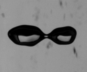
Figure 6. (a) Front view for a bubble of volume  $V=0.25$ cm
 $^{3}$ (
 $R_{eq}=3.9$ mm), at
  $\omega =89$ s
 $^{-1}$. (b) Same bubble and same conditions simultaneously recorded from side view.
2.3. Dimensionless parameters
We now wish to identify the parameters, and corresponding dimensionless numbers, needed to describe the equilibrium position and the shape of a bubble of volume  $V$ placed in a solid-body cylindrical rotational flow. As mentioned before, we assume the bubble is axisymmetric, and characterize its shape with two length scales: a length scale
  $L$ corresponding to the (supposedly larger) dimension of the bubble along the axis of rotation
  $z$, and the smaller length scale
  $D$, corresponding to the diameter of the bubble projection in a plane normal to the axis of rotation (see figure 1).
We introduce two dimensionless numbers to describe the shape of the bubble: the aspect ratio  $X=L/D$, which measures the stretching of the bubble, and the ratio
  $\alpha = V/(LD^{2})$. The latter characterizes the form of the bubble in a section containing the rotation axis
  $z$: it is for example expected to be equal to
  ${\rm \pi} /6$ if the bubble is an ellipsoid, or to
  ${\rm \pi} /4$ if the bubble is a cylinder. Note that the cylindrical shape is the limit shape predicted for very large
  $\omega$ in the model of Rosenthal (Reference Rosenthal1962).
The physical control parameters characterizing this problem are the liquid density  $\rho$, the acceleration due to gravity
  $g$, the rotational velocity of the tank
  $\omega$, the gas–liquid surface tension
  $\sigma$ and
  $\mu$, the dynamic viscosity of the liquid. In addition, we must consider the bubble position in the cross-section, which determines the flow around the bubble and hence the force exerted by the liquid upon on the bubble: we characterize this position with the coordinates of the bubble centre in polar coordinates, namely the distance
  $r_e$ to the axis of the cell, and the angle
  $\theta$ with the vertical direction (figure 7).

Figure 7. Bubble position in the cell cross-section: the centre of the bubble is characterized by  $r_e$ and
  $\theta$. The action of the liquid on the bubble is modelled as the sum of drag
  $\boldsymbol {F}_{\boldsymbol {D}}$, lift
  $\boldsymbol {F}_{\boldsymbol {L}}$, pressure and added mass
  $\boldsymbol {F}_{\boldsymbol {A}}$ contributions.
The above parameters can be grouped into five additional independent dimensionless numbers, which we choose to be the Rossby number  $Ro=r_e/D$, the Reynolds number
  $Re=\rho \omega r_e D/\mu$, the Froude number
  $Fr=\omega ^{2} r_e/g$, the Weber number
  $We=\rho \omega ^{2} D^{3}/8\sigma$ and the angle
  $\theta$.
Note that we have chosen to introduce a Reynolds number based on the mean velocity seen by the bubble. An alternative choice could be to introduce a Reynolds number based upon the shear seen by the particle
 \begin{equation} Re_{shear} = \dfrac{\rho \omega D^{2}}{\mu}=Re/Ro. \end{equation}
We will discuss in § 4 the relevance of this choice. The liquid–gas density and viscosity ratios can also be introduced. All experiments are here carried out with air and water, and since these two parameters are constant in the present study, we will not discuss them in the following.
The main control parameter driving the stretching of the bubble is expected to be  $We$, and similarly the forces acting on the bubble are expected to be mostly controlled by
  $Re$. We will show in the following sections that corrections in
  $Ro$ have to be introduced when the bubble approaches the axis of rotation of the cell.
3. Deformation of the bubble
We present in this section measurements of the aspect ratio of the bubble, defined as  ${X=L/D}$, as a function of
  $\omega$ and for a large range of bubble volumes
  $V$ (from 0.69 mm
 $^{3}$ to 0.27 cm
 $^{3}$). As expected, we observe that, when
  $\omega$ is increased, the bubbles are stretched along the axis of rotation (figures 5 and 6), and hence that their aspect ratio
  $X=L/D$ increases. Figure 8 shows the variations of
  $X$ as a function of
  $\omega$ for a large range of bubble volumes. The aspect ratio increases monotonically for almost all series, and reaches a value of 2.2 for the largest bubble investigated here and the largest
  $\omega$.

Figure 8. Variation of the aspect ratio  $X=L/D$ as a function of
  $\omega$.
The stretching results from the difference in pressure between the region of the bubble straddling the axis of rotation, where pressure is minimal, and the periphery of the bubble: as mentioned in the introduction this effect has been modelled by Rosenthal (Reference Rosenthal1962) in the limit of zero buoyancy and viscosity: within this assumption, the axisymmetric bubble centre stands on the cell axis of rotation. Relating the jump in pressure between the parabolic field outside the bubble and the constant pressure within the bubble as a function of the local curvature, and integrating relatively to the dimensionless distance to the axis  $\tilde {r}$ leads to (Rosenthal Reference Rosenthal1962)
 \begin{equation} X=\int_0^{1}\frac{\tilde{r}(1+(1-\tilde{r}^{2})We/8)}{(1-\tilde{r}^{2}(1+(1-\tilde{r}^{2})We/8)^{2})^{1/2}}\,\textrm{d}\tilde{r}. \end{equation}
This equation predicts that the aspect ratio  $X$ is a sole function of the Weber number.
Figure 9 shows the experimental data of figure 8, replotted as a function of the Weber number (same legend). The solid line corresponds to the prediction of (3.1). The aspect ratios of the different series in figure 8 are regrouped along the same curve in the  $(X,We)$ plane. However, the experimental aspect ratios are larger than the predicted one, and the relative departure to the prediction decreases when the Weber number is increased. This is directly related to the position of the bubble: the model assumes that the bubble centre lies on the axis of rotation, but in the experiment, buoyancy causes the bubble centre to be at a finite distance
  $r_e$ from this axis: the value of
  $r_e$ decreases when the Weber number is increased due to the steeper pressure gradient at larger rotational velocities, which explains the trend observed in figure 9.

Figure 9. Bubble aspect ratio as a function of Weber number. Same as in figure 8. The solid line corresponds to the model of Rosenthal (Reference Rosenthal1962).
The value of  $r_e$ is expected to be directly impacted by
  $\omega$ and
  $g$. We plot in figure 10 the dimensionless distance to the axis
  $r_e/D$, which is exactly the Rossby number
  $Ro$ introduced in § 2.3, as a function of
  $g/(D\omega ^{2})$. We see that
  $r_e/D$ is smaller than 1 for most of our experimental conditions, except for the smallest bubbles investigated. The error bars on this graph correspond to the standard deviation of
  $r_e$ values on the set of 255 images. In addition, figure 10 shows that the average
  $r_e$ can be estimated by
  $g/\omega ^{2}$. This is equivalent to saying that the Froude number introduced in § 2.3 is close to one for all our data. The data for the smallest bubble of
  $V=0.69$ mm
 $^{3}$ depart from this trend, and for this series,
  $r_e$ appears to be significantly smaller than
  $g/\omega ^{2}$ (and hence
  $Fr$ is significantly smaller than one): we will come back to the behaviour of this particular series in the next section. The value of
  $r_e$ is of course also expected to depend on the dimensionless quantities introduced in § 2.3, in particular the Reynolds number: this point will be discussed in the following section as well.

Figure 10. Value of  $Ro=r_e/D$ as a function of
  $g/D\omega ^{2}$. Same legend as in figure 8. The solid line indicates
  $Ro=g/D\omega ^{2}$.
When the bubble is centred, the pressure difference between the bubble periphery and axis is  $\Delta P_0=\rho \omega ^{2}D^{2}/8$ due to the parabolic pressure field. The fact that the bubble is shifted away from the axis of the cell at a finite
  $r_e$ means that the pressure difference it is submitted to will be larger than if it were centred on the axis. The minimum pressure exerted on the bubble will still be the pressure at the axis of the cell if
  $Ro<0.5$, which is the case for most of our data, except for smaller bubbles, but the average pressure around the periphery will be larger because of the convexity of the pressure profile in the solid-body rotation flow. It is easy to show by integration over the perimeter of the bubble that the pressure difference between the mean pressure at the periphery of the bubble and pressure on the axis of the rotating cell, for a bubble of diameter
  $D$ whose centre is displaced at a distance
  $r_e$ from the axis, will be given by
  $\Delta P=\Delta P_0(1+4r_e^{2}/D^{2})=\Delta P_0(1+4Ro^{2})$, see figure 11. This result can be rapidly recovered by just considering the mean pressure over the diameter represented by the dashed line in figure 11
 \begin{align} \Delta P&=\frac{P^{+}+P^{-}}{2}-P_{axis} = \frac{1}{4}\rho \omega^{2}\left(\left(r_e+\frac{D}{2}\right)^{2}+\left(r_e-\frac{D}{2}\right)^{2}\right)\nonumber\\ &=\frac{1}{8}\rho \omega^{2}D^{2}\left(1+\frac{4r_e^{2}}{D^{2}}\right). \end{align}
Figure 11. Sketch of the bubble of radius  $R$, illustrating pressures
  $P^{+}$ and
  $P^{-}$ at the surface of the bubble and their corresponding values on the parabolic pressure field in the tank. For a bubble shifted of a distance
  $r_e$ from the tank axis, the pressure difference between mean pressure at periphery and pressure on axis of the cell is
  $\Delta P= {(P^{+}+P^{-})}/{2}-P_{axis}$.
Because of this shift off the axis, the bubble is obviously not axisymmetric anymore, as supposed in the model of Rosenthal (Reference Rosenthal1962), and finding a generalization of (3.1) for the non-axisymmetric problem appears difficult. We propose to avoid this difficulty by considering that the displaced bubble is equivalent to a centred bubble rotating at a larger  $\omega '$ such that
  $\omega '=\omega (1+4r_e^{2}/D^{2})^{1/2}$, i.e. one which generates the actual pressure difference
  $\Delta P$ instead of
  $\Delta P_0$. This is equivalent to introducing a modified Weber number
  $We'=\rho \omega '^{2} D^{3}/8\sigma =We(1+4Ro^{2})$. Based on the results of figure 10, we estimate that
  $Ro\approx g/(D\omega ^{2})$, which yields
  $We'=We(1+4g^{2}/(D^{2}\omega ^{4}))$.
We plot in figure 12 the aspect ratio  $X$ as a function of this modified Weber number: even though there is still a slight underestimation of the aspect ratio for small bubbles, this improved model predicts relatively accurately the aspect ratio, in spite of the strong assumptions made on the shape of the bubble. The correction introduced by the Weber number correctly captures how buoyancy drives bubbles away from the axis of the cell at a finite
  $r_e$, and therefore exposes them to a steeper pressure gradient than the one they would experience if they were centred. The discrepancy observed for the very small bubbles may be related to the impact of the mean velocity
  $r_e \omega$ on the shape of the bubble: for these small bubbles, the Weber number
  $We_{re}=4We Ro^{2}$ built with the mean flow is larger than the Weber number introduced in § 2.3, which points to a possible distinct origin of the deformation for this case.


The data for the larger bubbles show a non-monotonic behaviour for the largest Weber numbers (a behaviour already present in figure 9): the decrease of the aspect ratio at larger  $We$ is correlated to a very strong increase in the fluctuations around the mean aspect ratio, as shown by the larger error bars for these points. These shape fluctuations, which will be discussed in the following section, are in addition associated with a strong increase in the fluctuations of the distance to the axis
  $r_e$. Our simple model based on the mean values of these quantities is probably not sufficient to capture the bubble shape for these non-stationary conditions. We will propose an explanation for the cause of these fluctuations in § 4.2.
A further explanation for the apparent underestimation of the aspect ratio  $X$ at large
  $We$ could reside in the method used for the determination of
  $D$, the mean diameter in the cross-section: we determine
  $D$ from front view projections, but for strongly distorted bubbles at large
  $We$ the size of this projection is certainly larger than the local
  $D$ at a given longitudinal position
  $z$. This will lead to an underestimation of
  $X$ and an overestimation of
  $We$ for strongly distorted bubbles.
4. Drag and lift coefficients
As mentioned in § 2, the bubbles move closer to the axis of rotation when  $\omega$ is increased. Their average position is characterized by the distance
  $r_e$ and the angle
  $\theta$ (see figure 7). The aim of this section is to deduce from measurements of the bubble position and shape how the forces acting on the bubble can be modelled in the present limit of large bubble sizes.
Following Magnaudet & Eames (Reference Magnaudet and Eames2000), we assume that the force exerted by the liquid on the bubble can be written as a superposition of the pressure gradient and added mass forces  $\boldsymbol {F}_{\boldsymbol {A}}$, drag force
  $\boldsymbol {F}_{\boldsymbol {D}}$, lift force
  $\boldsymbol {F}_{\boldsymbol {L}}$, plus of course buoyancy
  $\boldsymbol {F}_{\boldsymbol {B}}$ (figure 7), and write the equation of motion of the bubble of velocity
  $\boldsymbol {v}$ as
 \begin{equation} \rho V C_{A} \dfrac{\textrm{d}\boldsymbol{v}}{\textrm{d}t} = \rho V(C_{A} +1) \dfrac{\textrm{D}\boldsymbol{U}}{\textrm{D}t} + \boldsymbol{F}_{\boldsymbol{D}}+\boldsymbol{F}_{\boldsymbol{L}} -\rho V\boldsymbol{g}, \end{equation}
where  $\boldsymbol {U}$ is the velocity of the undisturbed ambient flow taken at the centre of the bubble.
As discussed in § 2, we study relatively large  $\omega$ such that the amplitude of oscillations around the bubble mean position remain small compared with the bubble size. We therefore neglect the variations of the velocity of the bubble, and the balance of forces on the bubble can be written (as in Rastello et al. Reference Rastello, Marié, Grosjean and Lance2009)
 \begin{equation} 0=V(C_A+1)\frac{\textrm{D}\boldsymbol{U}}{\textrm{D}t}+ \dfrac{1}{2} C_{D} A_{b} \lvert \boldsymbol{U}\rvert \boldsymbol{U}+ V C_{L} \boldsymbol{U} \times (\boldsymbol{\nabla} \times \boldsymbol{U}) -V\boldsymbol{g}, \end{equation}
where we have introduced the drag and lift coefficients  $C_D$ and
  $C_L$, and
  $A_b$, which is the projection of the bubble area normal to the
  $\hat {\boldsymbol {\theta }}$ direction. For an axisymmetric ellipsoidal bubble of axes
  $L$ and
  $D$ (figure 1b),
  $A_b={\rm \pi} LD/4$. The acceleration of the bubble in its limit cycle around the mean position can be estimated a posteriori from experimental results, and we could check that this term was smaller than the lift and drag contributions.
Here, the base flow is a solid-body rotation and the base flow  $\boldsymbol {U}$ at the centre of the bubble is
  $\omega r_e\hat {\boldsymbol {\theta }}$. The lift force is then
 \begin{equation} \boldsymbol{F}_{\boldsymbol{L}}=C_L2\rho V \omega^{2} r_e\hat{\boldsymbol{r}}. \end{equation}
The added mass and pressure forces both scale with the pressure gradient caused by the base flow  $\boldsymbol {U}$
 \begin{equation} \rho V(C_A+1)\frac{\textrm{D}\boldsymbol{U}}{\textrm{D}t}={-}V(C_A+1)\boldsymbol{\nabla} P={-}\rho V(C_A+1)\omega^{2}r_e\hat{\boldsymbol{r}}. \end{equation}
This contribution is of the same form as the lift contribution. The added mass coefficient can be computed as a function of the shape of the bubble, as will be shown further below.
Under the previous assumptions, the drag contribution can be written
 \begin{equation} \boldsymbol{F}_{\boldsymbol{D}}=\rho C_DA_b\tfrac{1}{2}U(r_e)^{2}\hat{\boldsymbol{\theta}}=\rho C_DA_b\tfrac{1}{2}r_e^{2}\omega^{2}\hat{\boldsymbol{\theta}}. \end{equation}
 The lift and drag coefficients are a priori not known, but their values  $C_L$ and
  $C_D$ can be deduced from the projections of (4.2) along
  $\hat {\boldsymbol {r}}$ and
  $\hat {\boldsymbol {\theta }}$
 \[\left\{ {\begin{array}{*{20}{l}} {({C_A} + 1) - 2{C_L} = \frac{g}{{{r_e}{\omega ^2}}}\cos \theta = \frac{1}{{{F_r}}}\cos \theta ,}\\ {\frac{{{C_D}}}{2} = \frac{{{V_g}}}{{{A_b}r_e^2{\omega ^2}}}\sin \theta = \frac{{\alpha \beta }}{{Ro{F_r}}}\sin \theta .} \end{array}} \right.\]
 This system shows that  $C_L$ is a function of
  $r_e$ via the Froude number
  $Fr$, and also of
  $\theta$ and
  $X$ via the added mass coefficient. The drag coefficient is a function of
  $Fr$,
$Fr$,  $\theta$,
  $Ro$,
$Ro$,  $\alpha =V/(LD^{2})$ and
  $\beta ={A_b}/{(LD)}$: the latter grouping is, similar to
  $\alpha$, a number characterizing the shape of the bubble;
  $\beta ={\rm \pi} /4$ for an ellipsoid and
  $\beta =1$ for a cylinder. At any rate,
  $\alpha$ and
  $\beta$ are not expected to vary much when the deformation of the bubble is moderate. In particular, for the range of aspect ratios investigated here (
 $1< X<2.2$), the model of Rosenthal (Reference Rosenthal1962) predicts that
  $\alpha$ varies between
  ${\rm \pi} /6\approx 0.52$ and 0.56, and that
  $\beta$ varies between
  ${\rm \pi} /4\approx 0.78$ and 0.82.
In order to check this experimentally, one possibility is to estimate  $\alpha$ directly from
  $V_0$,
  $L$ and
  $D$, by assuming that
  $V$ remains relatively close to the injected volume
  $V_0$, which should be true for lower
  $\omega$ values. We plot in figure 13(a) the variations of this estimate
  $\alpha _{inj}=V_0/LD^{2}$ as a function of
  $\omega$: the values are relatively close to the ellipsoid value
  ${\rm \pi} /6$ for all series (red dotted line), in particular for the lower value of
  $\omega$. It decreases down to 0.4 for the largest
  $\omega$. We interpret this decrease as caused by the fact that, at large
  $\omega$, the volume
  $V_0$ used for the calculation of
  $\alpha _{inj}$ is an underestimation of the actual volume
  $V$ of the stretched bubble.

Figure 13. (a) Coefficient  $\alpha _{inj}=V_0/(LD^{2})$ as a function of
  $\omega$. The red line indicates the value for an ellipsoid
  ${\rm \pi} /6$. The blue dashed line shows the value for a cylinder,
  ${\rm \pi} /4$. (b) Cartography of the conditions covered by the present experiments in the
  $(Re,Ro)$ plane. Same legend as in figure 8.
All in all, we observe that  $\alpha \approx {\rm \pi}/6\approx 0.52$ at the lower
  $\omega$. For larger
  $\omega$ we cannot check directly that this holds since the volume
  $V$ cannot be measured reliably from the two projections given the strong bubble deformations, and
  $\alpha _{inj}$ probably underestimates
  $\alpha$. The model of Rosenthal (Reference Rosenthal1962) predicts
  $\alpha =0.56$ for
  $\omega =94$ s
 $^{-1}$, i.e. a modest increase of approximately 7 % from the value at
  $\omega =63$ s
 $^{-1}$. In order to simplify the discussion, we assume in the following that
  $\alpha$ remains close to its value for an ellipsoid, i.e.
  ${\rm \pi} /6$ for all our conditions. Similarly, and in order to be consistent with this choice, we assume
  $\beta ={\rm \pi} /4$. This assumption may lead to a slight underestimation of the drag coefficient at large
  $\omega$, of at most 10 %. We then use system (4.6) to deduce
  $C_L$ and
  $C_D$ from the measurements of the bubble average position and shape.
Note that previous studies for air bubbles in water have been concerned with the values of  $C_L$ and
  $C_D$ as functions of
  $Re$ and for large
  $Ro$ (van Nierop et al. Reference van Nierop, Luther, Bluemink, Magnaudet, Prosperetti and Lohse2007; Rastello et al. Reference Rastello, Marié, Grosjean and Lance2009). The main difference for the large bubbles considered here is that we will consider low
  $Ro$, down to
  $Ro \approx 0.15$, when the bubble is close to the centre of the rotating cell. We illustrate in figure 13(b) the values of
  $Re$ and
  $Ro$ for all the measurements presented here.
4.1. Drag coefficient
We plot in figure 14(a) the drag coefficient, deduced from (4.6b) via measurements of the mean values of  $r_e$ and
  $\theta$, as a function of
  $Re$. The red solid line indicates the prediction of Schiller & Naumann (Reference Schiller and Naumann1933) for a solid sphere in a uniform flow. We have included in this graph the results of an additional measurement for a smaller bubble (grey asterisk,
  $V=0.50$ mm
 $^{3}$,
  $R_{eq}=0.5$ mm). For this particular bubble,
  $\omega$ is varied between 10 and 30 s
 $^{-1}$, and
  $Ro$ varies between respectively 10 and 3 in this interval, i.e. this bubble remains relatively far from the cell axis. We recover in this particular case previous results also obtained with demineralized water (Rastello et al. Reference Rastello, Marié, Grosjean and Lance2009, Reference Rastello, Marié and Lance2017); the points of this series fall close to the curve for solid spherical particles due to the inevitable presence of contaminants on the bubble interface. On the contrary, for larger bubbles closer to the cell centre, and which for most of them straddle the axis of rotation (
 $Ro<0.5$, see figure 13), we measure much larger drag coefficients, reaching values of up to 10. In addition, the scatter of the different series shows a strong influence of
  $Ro$ on
  $C_D$: for a given
  $Re$,
$Re$,  $C_D$ is larger for a larger bubble, i.e. for smaller
  $Ro$.
$Ro$.

Figure 14. (a) Drag coefficient  $C_{D}$ as a function of
  $Re$. (b) Drag coefficient
  $C_{D\varDelta }$ as a function of the shear Reynolds number
  $Re_{shear}$.
The large values of  $C_D$ show that expression (4.5) does not capture correctly the order of magnitude of the drag force at low
  $Ro$. A spinning wake is expected to envelop the bubble at this low
  $Ro$, and therefore the configuration is different from that at large
  $Ro$ where different orders of magnitude of the fluid force are expected to coexist perpendicular or along the wake direction. It seems reasonable to expect that, in the present vortex-like low
  $Ro$ limit, both lift and drag will be of similar orders of magnitude.
Another way to put it is to consider that the drag caused by the spinning wake around the bubble will be dominated by the dynamic pressure difference around the bubble; the order of magnitude of this difference is the difference between the (maximum) dynamic pressure at the point farthest from the origin and the (minimum) dynamic pressure at the point closest to the origin (see  $P^{+}$ and
  $P^{-}$ in figure 11), namely
 \begin{equation} \Delta P_d \approx P^{+}-P^{-}=\tfrac{1}{2}( \rho \omega^{2}(R+r_e)^{2}-\rho \omega^{2}(R-r_e)^{2})=2\rho \omega^{2} R r_e, \end{equation}
instead of  $\rho U(r_e)^{2}/2$ for the uniform flow limit. Instead of the classical form of the drag force in uniform flow (4.5), the proposed expression for the drag force is then
 \begin{equation} F_D=C_{D \varDelta}A_b\rho \omega^{2}Dr_e \hat{\boldsymbol{\theta}}, \end{equation}
where we have introduced a new drag coefficient  $C_{D \varDelta }=C_D Ro/2$. Note again that the order of magnitude introduced by (4.8) is larger than that of (4.5), since
  $r_e$ is smaller than
  $R$ for almost all our conditions (low
  $Ro$ limit). The scaling law for the drag force is then similar to that introduced for the other forces exerted by the fluid (added mass, pressure and lift force), in (4.3).
We plot in figure 14(b) the variations of  $C_{D \varDelta }$ as a function of
  $Re_{shear}$. The values of
  $C_{D\varDelta }$ are mostly in the range [0.6–0.9], which shows that the chosen definition captures the correct order of magnitude of the drag force. In addition, the data of figure 14(a) appear much better collapsed when plotted as in figure 14(b): for
  $Re_{shear}$ varying in the range [500–4000] we find an approximately constant
  $C_{D\varDelta }$ with
  $C_{D\varDelta } \approx 0.75$. This means that the classical drag coefficient can be estimated as
  $C_D\approx 2C_{D\varDelta }/Ro \approx 1.5/Ro$ at low
  $Ro$. An even simpler estimate for
  $C_D$ can then be built from this expression, by further assuming that
  $r_e\approx g/\omega ^{2}$ (valid for all series except the smaller
  $V=0.69$ mm
 $^{3}$ bubble, see figure 10), which yields
  $C_D\approx 1.5 D\omega ^{2}/g$. We plot in figure 15 the measured
  $C_D$ as a function of this simple prediction: the proposed expression manages to provide a relatively good estimate of the drag coefficient for the large range of conditions we investigate here. We believe the larger dispersion observed for large bubbles and large rotation rates is caused by larger fluctuations for these conditions. These fluctuations will be discussed in the following § 4.2.

Figure 15. Drag coefficient measured from bubble position, plotted as a function of proposed simplified model  $1.5D\omega ^{2}/g$: this prediction provides a good estimate of
  $C_D$ for the large range of conditions investigated here.
The data for the smaller bubble (black cross points) show much larger values of the drag coefficient  $C_{D\varDelta }$ in figure 14(b). This results from the fact that the measured
  $r_e\omega ^{2} /g$ for this series of points is smaller than for the other bubbles investigated, as mentioned above (figure 10). Indeed, for such a small bubble (
 $V=0.69$ mm
 $^{3}$,
  $R_{eq}=0.55$ mm), the values of
  $Re$ are significantly smaller: the reasoning behind the expression of (4.8) is not expected to be valid.
4.2. Lift
We show in figure 16 the variations of  $2C_L-C_A$, deduced from (4.6a), as a function of
  $Re$. In order to isolate the lift coefficient, and compare it with the results of the literature, we need to estimate the added mass coefficient. This coefficient can be computed analytically based on the measured shape of the bubble, provided the bubbles are assumed to be ellipsoidal. As mentioned above, the model of Rosenthal (Reference Rosenthal1962) predicts a small departure from the ellipsoidal shape, but this is assumed to be negligible here given the moderate deformation of the bubbles (coefficient
  $\alpha$ expected to increase from 0.52 to at most 0.56). The stretching of aspect ratio
  $X$ along the axis of the cell, which has been discussed in § 3, tends to increase the value of the added mass coefficient along the
  $\hat {\boldsymbol {r}}$ direction. However, the bubbles also tend to flatten slightly along
  $\hat {\boldsymbol {\theta }}$ due to the rotational flow when
  $Ro$ is not too small (figure 5a), and are therefore not strictly axisymmetric. The aspect ratio in the (
 $\hat {\boldsymbol {r}},\hat {\boldsymbol {\theta }}$) plane can reach values up to 1.4 for the largest bubbles and largest values of
  $We_{re}$, the Weber number based on the mean velocity
  $r_e\omega$: this flattening, even at moderate aspect ratios, is expected to decrease the added mass coefficient along
  $\hat {\boldsymbol {r}}$ compared with the axisymmetric assumption. We chose here to compute
  $C_A$ numerically from the mean bubble dimensions deduced from the visualizations: we assume that the bubbles are ellipsoidal, and integrate the expressions proposed by Lamb (Reference Lamb1934) (see Appendix A). The balance between the stretching along the axis of rotation (which increases
  $C_A$) and the more moderate flattening along
  $\hat {\boldsymbol {\theta }}$ (which reduces it) results in added mass coefficients relatively close to 0.5, i.e. close to those of a sphere. The increase of
  $C_A$ observed in figure 23(a) when bubble size is increased corresponds to the increase in
  $X$ for larger bubbles.


These computed added mass coefficients are then used to deduce  $C_L$: figure 17 shows the variations of the lift coefficient
  $C_L$ as a function of
  $Re$, and the comparison with some of the correlations introduced in Rastello et al. (Reference Rastello, Marié and Lance2017) for much larger
  $Ro$. The lift coefficient appears smaller than that measured by Bluemink et al. (Reference Bluemink, Lohse, Prosperetti and Van Wijngaarden2010) or Rastello et al. (Reference Rastello, Marié and Lance2017). The fact that
  $C_L$ is overestimated by these correlations could be caused by the smaller
  $Ro$ in our experiments: a decrease of the lift coefficient when
  $Ro$ is reduced has been observed by Rastello et al. (Reference Rastello, Marié and Lance2017) (see figure 20 of their paper). Note, however, that this decrease has been observed for
  $Ro>6$ i.e. bubbles located much farther from the axis. Bluemink et al. (Reference Bluemink, Lohse, Prosperetti and Van Wijngaarden2010) observed similar trends for spheres and investigated a few locations closer to the axis. They noted that
  $C_L$ decreased with the shear rate
  $Sr_{\omega }=Ro^{-1}$ up to
  $Sr_{\omega }=0.4\ (Ro=2.5)$ and that, after, the decrease stopped and
  $C_L$ became constant. This suggests that the influence of
  $Ro$ could also be limited in our case. The question of the limit of
  $C_L$ when
  $Ro$ becomes small therefore remains an open question.

Figure 17. Lift coefficient as a function of Reynolds number. The dashed and solid lines correspond to equations (B1)–(B2) and (B5) in Rastello et al. (Reference Rastello, Marié and Lance2017): black line, the bubble does not spin. The lift is only induced by the rotation flow, equations (B2)–(B5). Red line: the bubble is supposed to spin with the same rotation speed as the tank. This scenario is possible as the bubble is contaminated and located on the rotation axis. Rotation adds a contribution equal to 3/16, equation (B1). Equation (B2) is the correlation of the numerical results of Bluemink et al. (Reference Bluemink, Lohse, Prosperetti and Van Wijngaarden2010) for non-spinning sphere (code Physalis,  $Re \leq 200, Sr_{\omega }=Ro^{-1} \leq 0.1$); equation (B5) is the correlation of the experimental data of these authors for a non-spinning sphere (
 $Re >274, Sr_{\omega }=Ro^{-1} \leq 0.4$), with a different additional constant: 1.82 against 1.99 in Bluemink et al. (Reference Bluemink, Lohse, Prosperetti and Van Wijngaarden2010).
Besides the effect of  $Ro$, we know from the literature (Kariyasaki Reference Kariyasaki1987; Adoua, Legendre & Magnaudet Reference Adoua, Legendre and Magnaudet2009; Rastello et al. Reference Rastello, Marié and Lance2017; Hayashi et al. Reference Hayashi, Legendre and Tomiyama2020) that bubble deformation can yield a decrease of the lift force and can even make this force change sign from positive to negative. Even though the main bubble stretching is aligned with the rotation axis, larger bubbles are actually also deformed in the
  $(r,\theta )$ plane, see figure 5 for example: for these non-axisymmetric cases, bubble deformation certainly affects the value of the lift coefficient. Note finally that the motion of the bubble around its equilibrium position may increase the inertia of the surrounding fluid, and hence lead to an increase in the effective added mass: the data of figure 17, which do not take this effect into account, are therefore expected to represent an underestimation of
  $C_L$.
When experiments are performed in demineralized water, as used here, the surface of the bubble is contaminated and in this case it is expected to ‘spin’. This has been shown for small bubbles at equilibrium far from the axis of rotation ( $Ro \geq 6$) by tagging the flow near their surface with small fluorescent particles, in Rastello et al. (Reference Rastello, Marié, Grosjean and Lance2009) and Rastello et al. (Reference Rastello, Marié and Lance2017). Visualizations show that fluorescent particles located very close to the bubble surface (the distance is smaller than 50
  $\mathrm {\mu }$m in figure 14 of Rastello et al. Reference Rastello, Marié, Grosjean and Lance2009) rotate around the bubble. These authors assimilate the motion of the fluid close to the surface to the rotation of the surface itself, and speak of a ‘spinning’ surface. For bubbles with
  $Ro\geq 6$, the mean spinning rate is higher than the rotation rate: up to 1.6, depending on
  $Re$ (figure 10 in Rastello et al. Reference Rastello, Marié and Lance2017). This results in an extra Magnus-like lift force and a separated wake behind the bubble whose description can be found in Rastello & Marié (Reference Rastello and Marié2020).
In the present case, bubbles stabilize on average on, or very close to, the rotation axis ( $Ro<1$). It is probable that, if spinning, they will spin at most with the rotation rate of the tank and not faster (see figure 3 in Bluemink et al. Reference Bluemink, Lohse, Prosperetti and Van Wijngaarden2008 for spheres), which will result in an extra Magnus-like lift coefficient of at most the order of 3/16. Figure 17 shows that the present lift coefficients mostly lie below the values expected for non-spinning bubbles (indicated by the black curve): we believe this discrepancy with previous models is due to the effect of
  $Ro$, which is much smaller in our case than in previous studies.
When the bubble moves closer to the axis of rotation at low  $Ro$, and in particular when it straddles the axis of rotation of the cell, the flow configuration changes: the relative importance of the shear increases, and the relevant Reynolds number is expected to become at some point the shear Reynolds number
  $Re_{shear}=Re/Ro$ introduced in §§ 2.3 and 4.1. We plot in figure 18 the variations of the lift coefficient
  $C_L$ as a function of
  $Re_{shear}$: the data of figure 17 appear better collapsed. The decrease of
  $C_L$ observed in the range
  $Re_{shear}=500 - 2500$ is consistent with the decrease observed by Rastello et al. (Reference Rastello, Marié and Lance2017) when
  $Ro^{-1}$ is increased, and when the Reynolds dependence is accounted for.

Figure 18. Lift coefficient as a function of shear Reynolds number,  $Re_{shear}=Re/Ro$. The greyed region corresponds to conditions where the bubble experiences strong shape fluctuations.
A sharp transition seems to occur for large bubbles when  $Re_{shear}$ becomes larger than 2800 (greyed region in figure 18). Imaging of the bubble motion just before and after this transition indicates that the apparent increase in
  $C_L$ is associated with a strong periodic stretching of the bubble, synchronized with the rotation of the tank. We show in figure 19 how the increase in the lift coefficient appears correlated with the strong increase of the variance of the longitudinal aspect ratio
  $X$. The strong increase of these fluctuations appears related to a forcing of the bubble stretching by the rotation of the tank (see supplementary movie 1 available at https://doi.org/10.1017/jfm.2021.683). We introduce
  $\omega _0=\sqrt {12\sigma /\rho L^{3}}$ as an estimate of the eigenfrequency of the stretched bubble (Risso Reference Risso2000): as
  $\omega$ is increased,
  $\omega _0$ decreases due to the stretching of the bubble and
  $\omega$ and
  $\omega _0$ eventually coincide. Figure 19(b) shows that the transition observed around
  $Re_{shear}=3000$ in figure 18 corresponds precisely to
  $\omega /\omega _0 \approx 1$. The resonance expected for these conditions may explain the strong increase observed in the fluctuations of the aspect ratio.

Figure 19. (a) Lift coefficient as a function of the variance of the longitudinal aspect ratio  $X$. (b) Lift coefficient as a function of the ratio between the tank rotation frequency and the eigenfrequency of the stretched bubble
  $\omega _0$.
The question is then why the resonance provokes this steep apparent variation in the lift coefficient. A possibility could be that this apparent increase is caused by the much larger fluctuations in the position for these larger bubbles. Relative variations of  $r_e$ can reach up to 30 %–40 % when resonance occurs, compared with less than 10 % for all series of bubbles with
  $Re_{shear}<2500$. These fluctuations in position are probably themselves triggered by the strong fluctuations in the shape of the bubbles. At any rate, because of these large fluctuations in
  $r_e$, mean values of
  $C_L$ for
  $Re_{shear}>2500$ deduced from the mean position result in fact from the averaging of a strongly non-stationary dynamics, something which is not accounted for in the equations leading to system (4.6).
Imaging of the bubble motion shows that the strong oscillations caused by the resonance strongly distort the bubble, which may then exhibit non-axisymmetric deformations. As illustrated in figure 20, these oscillations can even lead to the rupture of the bubble into two fragments of similar size; see also supplemental movie 2. This is only observed for the largest bubbles ( $V>0.25$ cm
 $^{3}$) and largest
  $\omega$ investigated. The study of the conditions for break-up, and more generally of the dynamics of the bubble when the rotation of the cell forces its eigenmodes, is left for future work.

Figure 20. Series of images showing the break-up of a bubble of volume  $V=0.27$ cm
 $^{3}$ (
 $R_{eq}=0.4$ cm), at
  $\omega =84$ s
 $^{-1}$.
5. Conclusion
We have obtained experimental results regarding the shape of a bubble placed in a horizontal solid body rotational flow, for conditions of low  $Ro$, namely for bubbles close to the axis of rotation, at high rotation speeds. We have shown in § 3 that the model of Rosenthal (Reference Rosenthal1962) adequately captures the stretching of the bubble when its Weber number is increased, provided a correction accounting for the finite distance to the cell axis and the impact this has on the mean pressure field around the bubble, is included. This model relies on the assumption that the bubble is axisymmetric: even though this is not the case when buoyancy breaks the symmetry, the correction we propose is sufficient to capture the aspect ratio of the bubble in a wide range of conditions.
We have shown in § 4.1 values for the drag coefficient of the bubble, deduced from measurements of the bubble position: these results show that, as  $Ro$ becomes smaller than 1, the drag coefficient increases and the impact of
  $Ro$ becomes more pronounced. We have shown that for bubbles straddling the axis of the cell, the drag coefficient could be simply approximated by
  $C_D\approx 1.5/Ro$. If we further consider that, for the large bubbles considered here
  $r_e \approx g/\omega ^{2}$, this is equivalent to predicting
  $C_D\approx 1.5 D\omega ^{2}/g$ for such bubbles in this regime, a simple expression which captures well the order of magnitude of
  $C_D$ for almost all our experimental conditions.
Finally, we have proposed in § 4.2 an estimate of the lift coefficient for the low  $Ro$ limit. This lift coefficient seems to be controlled by the shear Reynolds number when
  $Re_{shear}=Re/Ro$ is in the range [500–3000], conditions for which one may expect an inertial wake to surround the bubble. In this range,
  $C_L$ is of the order of 0.5, and decreases slightly when the Rossby number is reduced (i.e.
  $Re_{shear}$ is increased). We observe a transition above
  $Re_{shear}=3000$, above which the bubble exhibits strong oscillations in shape and position. We believe these oscillations are caused by a resonance between the driving frequency
  $\omega$ and the eigenfrequency
  $\omega _0$ of the bubble, a resonance which occurs above a given
  $\omega$ depending on bubble size, due to the decrease of
  $\omega _0$ as the bubble is stretched along the axis of rotation. This resonance can lead to the break-up of the bubble. Investigation of the conditions for which this break-up occurs and of the probable coupling with the non-stationary dynamics of the bubble will be the scope of future studies.
Supplementary movies
Supplementary movies are available at https://doi.org/10.1017/jfm.2021.683.
Acknowledgements
We acknowledge fruitful discussions with the late Professor P. Spelt.
Funding
This research was supported by the French Agence Nationale de la Recherche ANR under grant no. SURFBREAK ANR-18-CE08-0013.
Declaration of interest
The authors report no conflict of interest.
Appendix A. Variations of the added mass coefficient as a function of aspect ratio and Weber number
The added mass coefficients of an ellipsoid moving in an infinite fluid can be found in Lamb (Reference Lamb1934). They are obtained by calculating the motion of a liquid, at rest at infinity, produced by the translation of a solid ellipsoid through it. The ellipsoid is characterized by the half-lengths  $a$,
$a$,  $b$,
$b$,  $c$ of its principal axes. We suppose that the half-length
  $c$ is aligned with the axis of rotation of the cell,
  $z$, and that directions
  $a$ and
  $b$ make an angle
  $\gamma$ with
  $\hat {\boldsymbol {r}}$ and
  $\hat {\boldsymbol {\theta }}$ respectively (see figure 21). We wish here to calculate the added mass coefficient relevant for (4.6a) which is the added mass coefficient along
  $\hat {\boldsymbol {r}}$. This coefficient, which is simply noted
  $C_A$ in the rest of the paper, will be noted more precisely
  $C_{Ar}$ in this appendix to avoid any ambiguity. The solution of motion with the use of special orthogonal curvilinear coordinates yields for added mass coefficients along axes
  $a$ and
  $b$
$b$
 \begin{equation} \left.\begin{aligned} C_{A a}=\frac{\alpha_0}{2-\alpha_0} \quad \mathrm{where} \ \alpha_0=abc \int_0^{\infty} \frac{\textrm{d}\lambda}{(a^{2}+\lambda)\varDelta},\\ C_{A b}=\frac{\beta_0}{2-\beta_0} \quad \mathrm{where} \ \beta_0=abc \int_0^{\infty} \frac{\textrm{d}\lambda}{(b^{2}+\lambda)\varDelta}, \end{aligned}\right\} \end{equation}
with  $\varDelta =((a^{2}+\lambda )(b^{2}+\lambda )(c^{2}+\lambda ))^{{1}/{2}}$.

Figure 21. Sketch showing the cross-section for an ellipsoidal bubble inclined of an angle  $\gamma$ relative to the cylindrical frame.
If we assume that the bubble is axisymmetric with  $a=b=D/2$ in the
  $(r,\theta )$ plane, and stretched by pressure effects along
  $z$ (with therefore
  $c> a = b$), coefficients
  $\alpha _0$ and
  $\beta _0$ are equal and can be expressed as a function of the aspect ratio
  $X=L/D=c/a$
 \begin{equation} \alpha_0=\beta_0=X \int_0^{\infty} \frac{\textrm{d}\lambda}{(1+\lambda)\varDelta_X}, \end{equation}
where  $\varDelta _X=(1+\lambda )(X^{2}+\lambda )^{{1}/{2}}$. Values of
  $X$ larger than one (corresponding to prolate ellipsoids) yield added mass coefficients
  $C_{A r}=C_{Aa}=C_{Ab}$ larger than 0.5, since the stretching along
  $z$ tends to increase inertia in the radial direction. This is illustrated in figure 22(a) on the blue dashed curve.

Figure 22. (a) Added mass coefficient  $C_{Ar}$ as a function of aspect ratio
  $X$, for different values of aspect ratio
  $X_{r\theta }$, and for
  $\gamma =0$. (b) Cartography showing the values of
  $We_{re}$ as function of
  $Re$ for each of our experimental conditions.
If we now drop the axisymmetric assumption, we are in a situation where a priori  $c>a>b$. Let the two aspect ratios be
  $X=c/b$ and
  $X_{r\theta }=a/b$. Coefficients
  $\alpha _0$ and
  $\beta _0$ are given by
 \begin{equation} \alpha_0=X X_{r\theta} \int_0^{\infty} \frac{\textrm{d}\lambda}{(X_{r\theta}^{2}+\lambda)\varDelta'} \quad \mathrm{and} \quad \beta_0=X X_{r\theta} \int_0^{\infty} \frac{\textrm{d}\lambda}{(1+\lambda)\varDelta'}, \end{equation}
with  $\varDelta '=((X_{r\theta }^{2}+\lambda )(X^{2}+\lambda )(1+\lambda ))^{{1}/{2}}$. The added mass coefficient along direction
  $\hat {\boldsymbol {r}}$ can then be computed as
  $C_{Ar}=C_{Aa}\cos ^{2} \gamma +C_{Ab}\sin ^{2} \gamma$. Figure 22 shows the variation of
  $C_{Ar}$ as a function of both aspect ratio, for the particular case
  $\gamma =0$, which is the value we observe experimentally for most bubbles except larger ones. As illustrated in figure 22, when
  $X_{r\theta }$ is increased for fixed
  $X$ the added mass coefficient decreases. Note that the assumption
  $\gamma =0$ is only made for figure 22(a) in order to simplify the discussion, and that in the data of figure 17,
  $\gamma$ has been experimentally measured for each bubble and
  $\omega$ via image processing. Note also that when
  $\gamma \neq 0$, and because of the non-diagonality of the added mass matrix, an additional added mass term should be introduced in (4.6b) and subsequently in the expression for the drag coefficient. Given the weak non-axisymmetry we observe in our data, this additional contribution is always small, and we do not discuss it here.
We show in figure 23(a) the variations of the added mass coefficient  $C_{Ar}$ as a function of Weber number
  $We$, which compares the pressure difference between periphery and axis with the capillary pressure (see § 3):
  $C_{Ar}$ increases with
  $We$, due to the increase in
  $X$ when
  $We$ is increased. The values of
  $X_{r\theta }$, which also impacts
  $C_{Ar}$, are on the contrary expected to increase with
  $We_{re}=\rho (r_e \omega )^{2}R/\sigma =4We Ro^{2}$, built with the mean velocity
  $r_e\omega$ seen by the bubble. As expected, the added mass
  $C_{Ar}$ decreases when
  $We_{re}$ is increased (figure 23b) for a given series (i.e. given range of
  $X$).
$X$).

Figure 23. (a) Added mass coefficient  $C_{Ar}$ as a function of Weber number
  $We$. The increase of
  $We$ leads to an increase of
  $X$, and then to an increase in
  $C_{Ar}$. (b) Value of
  $C_{Ar}$ as a function of
  $We_{re}$, which measures the impact of mean velocity
  $r_e\omega$ on the shape of the bubble. For a given series, the added mass decreases when
  $We_{re}$ is increased due the increase in
  $X_{r\theta }$.
The balance between the opposite roles of both aspect ratio results in added mass coefficients close to 0.5 for most bubbles investigated here. For the largest bubbles the added mass coefficient is a bit larger, closer to 0.7: these bubbles usually exhibit an angle  $\gamma$ of the order of
  ${\rm \pi} /4$, as in the sketch of figure 21 and also in the front view images of figures 5 and 6, which explains the larger inertia along
  $\hat {\boldsymbol {r}}$ in this case.
Note finally that the values of  $We_{re}$ in figure 22(b) are smaller than one for almost all conditions, which suggests that the axisymmetric approximation used throughout this paper, except for the added mass calculation, is reasonable.


