


1. Introduction
Bedload transport, the coarser sediment load transported by the water flow in close contact with the mobile river bed, is a major process that shapes the Earth's surface with consequences for public safety, water resources, territorial development and fluvial ecology. In mountain streams with steep slopes, large quantities of a wide range of grain sizes are transported, leading to grain size sorting, more generally named size segregation. Size segregation remains a poorly understood phenomenon (Gray Reference Gray2018) impairing our ability to model the interplay between sediment transport rates and channel morphological evolution such as armouring (Bathurst Reference Bathurst2007), bedload sheets (Venditti et al. Reference Venditti, Dietrich, Nelson, Wydzga, Fadde and Sklar2010; Bacchi et al. Reference Bacchi, Recking, Eckert, Frey, Piton and Naaim2014), patching (Nelson, Dietrich & Venditti Reference Nelson, Dietrich and Venditti2010) or downstream fining (Paola et al. Reference Paola, Parker, Seal, Sinha, Southard and Wilcock1992). The physics of granular media has been advocated to address segregation at the granular scale and understand geomorphological evolution (Frey & Church Reference Frey and Church2009, Reference Frey and Church2011). Size segregation largely originates from local interparticle interactions but has huge consequences for the particle size repartition both in the downward and streamwise directions over a much larger scale, potentially affecting sediment mobility and the entire channel geomorphological equilibrium (Gilbert & Murphy Reference Gilbert and Murphy1914; Ferguson et al. Reference Ferguson, Church, Rennie and Venditti2015; Dudill, Frey & Church Reference Dudill, Frey and Church2017; Dudill et al. Reference Dudill, Lafaye de Micheaux, Frey and Church2018, Reference Dudill, Venditti, Church and Frey2020). While investigating segregation at the granular scale (usually with discrete methods) is invaluable (Hill & Tan Reference Hill and Tan2014; Ferdowsi et al. Reference Ferdowsi, Ortiz, Houssais and Jerolmack2017; Chassagne et al. Reference Chassagne, Maurin, Chauchat, Gray and Frey2020b), it is also necessary to consider continuum modelling to improve our theoretical understanding and to provide predictions at larger scales. The focus of this paper is therefore to bridge the gap between the granular-scale processes and continuum modelling, by determining closures based on local granular mechanisms.
This contribution focuses on vertical size segregation processes due to kinetic sieving and associated squeeze expulsion (Savage & Lun Reference Savage and Lun1988; Gray Reference Gray2018). The moving particles act as a random fluctuating sieve, in which small particles are more likely to percolate under the action of gravity than larger particles. This downward movement is balanced by an upward squeeze expulsion which equally applies on small and large particles, resulting in a net downward motion of the small particles. The combination of both processes is called gravity-driven segregation (Gray Reference Gray2018) and is the dominant mechanism in bedload transport. Beyond the few studies made on size segregation in bedload transport (Hergault et al. Reference Hergault, Frey, Métivier, Barat, Ducottet, Böhm and Ancey2010; Ferdowsi et al. Reference Ferdowsi, Ortiz, Houssais and Jerolmack2017; Lafaye de Micheaux, Ducottet & Frey Reference Lafaye de Micheaux, Ducottet and Frey2018; Frey et al. Reference Frey, Lafaye de Micheaux, Bel, Maurin, Rorsman, Martin and Ducottet2020; Chassagne et al. Reference Chassagne, Frey, Maurin and Chauchat2020a,Reference Chassagne, Maurin, Chauchat, Gray and Freyb), these processes have been studied experimentally and numerically in many granular flows such as dry granular avalanches (Savage & Lun Reference Savage and Lun1988; Dolgunin & Ukolov Reference Dolgunin and Ukolov1995; Wiederseiner et al. Reference Wiederseiner, Andreini, Epely-Chauvin, Moser, Monnereau, Gray and Ancey2011; Jones et al. Reference Jones, Isner, Xiao, Ottino, Umbanhowar and Lueptow2018; Thornton, Gray & Hogg Reference Thornton, Gray and Hogg2006; Guillard, Forterre & Pouliquen Reference Guillard, Forterre and Pouliquen2016), shear cells (Golick & Daniels Reference Golick and Daniels2009; van der Vaart et al. Reference van der Vaart, Gajjar, Epely-Chauvin, Andreini, Gray and Ancey2015) or annular rotating drums (Thomas Reference Thomas2000).
While particularly complex segregation phenomena were observed (Thomas Reference Thomas2000), size segregation has been found to be mainly related to the forcing, the size ratio and the fine particle volume fraction. Savage & Lun (Reference Savage and Lun1988) predicted from dimensional analysis that the shear rate  $\dot {\gamma }^p$ should be the controlling parameter for size segregation. Indeed, when a granular medium is sheared, a layer of particles moves relatively faster than the one beneath, allowing particles to find gaps in which to fall by gravity. This theory agrees with experimental bi-disperse flow down inclined planes (Savage & Lun Reference Savage and Lun1988). In more recent works, Golick & Daniels (Reference Golick and Daniels2009) with shear cell experiments, and Fry et al. (Reference Fry, Umbanhowar, Ottino and Lueptow2018) with shear cell discrete element model (DEM) simulations, evidenced the effect of granular pressure, observing less efficient segregation when increasing the pressure. Gray (Reference Gray2018) suggested that size segregation depends on the inertial number, classically used to describe granular rheology (GDR MiDi 2004; da Cruz et al. Reference da Cruz, Emam, Prochnow, Roux and Chevoir2005),
 \begin{equation} I = \dfrac{d_l \dot{\gamma}^p}{\sqrt{p^p/\rho^p}}, \end{equation}
where  $d_l$ is the large particle diameter,
  $\dot {\gamma }^p$ is the granular shear rate,
  $p^p$ is the granular pressure and
  $\rho ^p$ is the particle density. DEM simulations of dry granular flows (Fry et al. Reference Fry, Umbanhowar, Ottino and Lueptow2018) and turbulent bedload transport (Chassagne et al. Reference Chassagne, Maurin, Chauchat, Gray and Frey2020b) have shown that the segregation velocity indeed scales with the inertial number to a power
  $0.845\pm 0.05$ from quasi-static to dense granular flow regimes.
Not surprisingly, a number of studies have also found that the segregation depends on the particle size ratio in the kinetic sieving regime. As kinetic sieving is related to the gaps created by shearing, it appears logical that it should be related to the size ratio. However, while Chassagne et al. (Reference Chassagne, Maurin, Chauchat, Gray and Frey2020b) have found that segregation increases monotonically with the size ratio in quasi-static regimes ( $I<10^{-3}\text {--}10^{-2}$) for size ratio up to 3, Golick & Daniels (Reference Golick and Daniels2009), Guillard et al. (Reference Guillard, Forterre and Pouliquen2016) and Jing et al. (Reference Jing, Ottino, Lueptow and Umbanhowar2020) found that it experiences a maximum efficiency for a size ratio of two,
  $r=2$, for more dynamic granular regimes (
 $10^{-3} < I < 1$). Yet, there is still no satisfying theory that explains this difference.
Similarly to the hindrance function for the fluid drag force on a particle, size segregation has also been observed to depend on the concentration of fine particles. Indeed, studies indicate that the efficiency of the segregation process is linked to concentration in small (or large) particles in the granular sample (Fan et al. Reference Fan, Schlick, Umbanhowar, Ottino and Lueptow2014a; van der Vaart et al. Reference van der Vaart, Gajjar, Epely-Chauvin, Andreini, Gray and Ancey2015; Jones et al. Reference Jones, Isner, Xiao, Ottino, Umbanhowar and Lueptow2018).
Size segregation can be analysed from a particle-scale mechanistic point of view, or a continuum one. On the one hand, considering a large particle in a bath of small particles, size segregation can be seen as a force destabilising the large particle and leading to a migration with respect to the small particles. A number of authors have adopted this approach and have shown that a particle experiences different kind of forces linked to size segregation (Ding, Gravish & Goldman Reference Ding, Gravish and Goldman2011; Tripathi & Khakhar Reference Tripathi and Khakhar2013; Guillard et al. Reference Guillard, Forterre and Pouliquen2016; Staron Reference Staron2018; van der Vaart et al. Reference van der Vaart, van Schrojenstein Lantman, Weinhart, Luding, Ancey and Thornton2018). The forces can be decomposed into a component that drives the segregation and a resulting resisting component linked to the relative motion of the large particle with respect to the small. These two different forces have been isolated by Guillard et al. (Reference Guillard, Forterre and Pouliquen2016) and Tripathi & Khakhar (Reference Tripathi and Khakhar2013). To assess the segregation forces due to the particle size differences, Guillard et al. (Reference Guillard, Forterre and Pouliquen2016) performed two-dimensional (2-D) DEM simulations of a large disk placed in a bed of small disks in the simple shear flow configuration. Maintaining the large disk at a given position with a virtual spring, they were able to assess the vertical segregation force applied by the small particles to the large one,  $f_{seg}$, without generating a resisting force due to the particle motion. Guillard et al. (Reference Guillard, Forterre and Pouliquen2016) found that the vertical segregation force has two contributions: one proportional to the pressure gradient
  $\partial p^p / \partial z$ arising from the enduring contact between particles; the other proportional to the granular shear stress gradient
  $\partial {|\tau ^p|}/\partial {z}$
 \begin{equation} f_{seg} = V_l \left(\mathcal{F}(\mu,r) \displaystyle\frac{\partial p^p}{\partial z} + \mathcal{G}(\mu,r) \dfrac{\partial{|\tau^p|}}{\partial{z}} \right), \end{equation}
where  $V_l = {\rm \pi}d_l^{3}/6$ is the volume of the intruder and
  $\mathcal {F}$ and
  $\mathcal {G}$ are empirical functions depending on the friction coefficient
  $\mu = |\tau ^p|/p^p$ and on the size ratio
  $r = d_l/d_s$ between the intruder and the surrounding small particles. Guillard et al. (Reference Guillard, Forterre and Pouliquen2016) studied the dependency on both parameters but only provided a dependency with
  $\mu$ as
 \begin{equation} \mathcal{F}(\mu) \!=\! 2.4 + 0.73 \exp\left({ -\frac{(\mu-\mu_c)}{0.051}}\right) \quad \text{and} \quad \mathcal{G}(\mu) ={-} \left(2+ 5.5 \exp\left({ -\frac{(\mu-\mu_c)}{0.076}}\right)\right), \end{equation}
where  $\mu _c$ is the critical friction coefficient defining the threshold of movement. It appears that the segregation force proposed in (1.2) accounts for a granular buoyancy force that counter-balances the weight of the particle and a granular lift force arising from multiple inter-particle contact interactions with the intruder (Guillard, Forterre & Pouliquen Reference Guillard, Forterre and Pouliquen2014). Hence the dependencies (1.3a,b) result from the measurements of both these forces.
Tripathi & Khakhar (Reference Tripathi and Khakhar2013) performed 3-D DEM simulations of a settling heavy sphere in a bed of lighter spheres, during a steady dry granular flow on an inclined plan. This density segregation set-up generates a relative motion between the heavy sphere and the lighter ones, without generating segregation forces due to size ratio. By analogy with classical hydrodynamics, light particles playing the role of an ambient fluid, the authors showed that the interaction force could be modelled with a Stokesian form of a solid drag force
 \begin{equation} f^{p}_{d} = c(\varPhi) {\rm \pi}\eta^{p} d_l v, \end{equation}
where  $v$ is the settling velocity of the heavier particle,
  $c(\varPhi )$ is a drag coefficient depending on the local solid volume fraction
  $\varPhi$ and
  $\eta ^p = |\tau ^p|/|\dot {\gamma }^p|$ is the viscosity of the granular medium considered as a non-Newtonian fluid. Tripathi & Khakhar (Reference Tripathi and Khakhar2013) suggested that
  $c(\varPhi )$ depends on the local volume fraction
  $\varPhi$ but still remains of the same order as the value observed for a Stokes law in Newtonian fluids, i.e.
  $c=3$. These two forces allow one to understand particle migration locally, and to relate the segregation behaviour of particles to the local characteristics of the granular flow.
By contrast, addressing the effect of size segregation processes at the large scale requires a different approach that disregards the particles. Such an approach has been extensively developed in the last few years focusing on a description of segregation as an advection–diffusion model for the percolation of small particles (Dolgunin, Kudy & Ukolov Reference Dolgunin, Kudy and Ukolov1998; Gray & Chugunov Reference Gray and Chugunov2006; Thornton et al. Reference Thornton, Gray and Hogg2006; Hill & Tan Reference Hill and Tan2014; van der Vaart et al. Reference van der Vaart, Gajjar, Epely-Chauvin, Andreini, Gray and Ancey2015; Ferdowsi et al. Reference Ferdowsi, Ortiz, Houssais and Jerolmack2017; Gray Reference Gray2018; Cai et al. Reference Cai, Xiao, Zheng and Zhao2019; Fry et al. Reference Fry, Umbanhowar, Ottino and Lueptow2019; Umbanhowar, Lueptow & Ottino Reference Umbanhowar, Lueptow and Ottino2019)
 \begin{equation} \dfrac{\partial \phi^s}{\partial t} - \dfrac{\partial}{\partial z}\left(\phi^s w_s\right) = \dfrac{\partial}{\partial z}\left(D \dfrac{\partial \phi^s}{\partial z} \right), \end{equation}
where  $t$ denotes for time,
  $z$ the vertical axis,
  $\phi ^s$ and
  $\phi ^l$ are the small and large particle concentrations and sum to unity (with
  $\phi ^s+\phi ^l = 1$),
  $w_s$ is the advection velocity of segregation and
  $D$ is the diffusion coefficient. This equation is characterised by the segregation flux
  $\phi ^s w^s$, and the advective velocity
  $w^s$, which encompass the physical dependencies of the size segregation discussed previously. The advective velocity should therefore have a dependence on the local concentration, which is classically taken as proportional to the large particle concentration,
  $w_s=\phi ^l S_r$ (Dolgunin & Ukolov Reference Dolgunin and Ukolov1995; Gray & Thornton Reference Gray and Thornton2005). Here,
  $S_r$ is the advection coefficient of small particles into large particles. The latter has usually been taken as an empirical constant for a given application, or determined from a semi-empirical analysis. Based on a dimensional analysis and DEM simulations, Chassagne et al. (Reference Chassagne, Maurin, Chauchat, Gray and Frey2020b) showed that it should depend on both the inertial number and the size ratio. The diffusion coefficient
  $D$ models the diffusive remixing of small particles into large particles. The diffusion coefficient has also received attention in the literature (Bridgwater, Foo & Stephens Reference Bridgwater, Foo and Stephens1985; Fan et al. Reference Fan, Umbanhowar, Ottino and Lueptow2015; Fry et al. Reference Fry, Umbanhowar, Ottino and Lueptow2019). It has been suggested that it should depend on the volume fraction (Cai et al. Reference Cai, Xiao, Zheng and Zhao2019) and on the inertial number (Chassagne et al. Reference Chassagne, Maurin, Chauchat, Gray and Frey2020b).
Developing a three-phase continuum mixture theory to model a bi-disperse combination of large and small particles with an interstitial passive fluid, Thornton et al. (Reference Thornton, Gray and Hogg2006) and Gray & Chugunov (Reference Gray and Chugunov2006) were able to analytically derive the advection–diffusion model (1.5). This derivation represented an important step in the understanding of the physical processes at work in size segregation since the advection and diffusion coefficients of the advection–diffusion equation were linked to the particle-scale interactions. In particular, the derivation is based on the assumption that the size segregation directly takes its origin in the heterogeneous distribution of the granular pressure between small and large particles. However, the form of the interaction forces between large and small particles have been postulated without support from independent physical evidence.
This literature review evidences the absence of a direct link between the continuum modelling of grain-size segregation and the local segregation forces experienced by a grain. In this context, the aim of the present paper is to bridge the gap between the granular-scale approach and the continuum modelling. Based on the particle-scale forces proposed by Guillard et al. (Reference Guillard, Forterre and Pouliquen2016) and Tripathi & Khakhar (Reference Tripathi and Khakhar2013), a volume-averaging approach (Jackson Reference Jackson1997, Reference Jackson2000) is adopted here to derive a multi-phase continuum model from granular-scale forces. In addition to the novelty of the developed approach, the derivation proposed by Thornton et al. (Reference Thornton, Gray and Hogg2006) is used to express the advection–diffusion equation from the new multi-phase flow model, providing improved formulations of the advection and diffusion coefficients that contain the particle-scale granular dependencies. In order to test the proposed models, the bi-disperse turbulent bedload transport configurations investigated in Chassagne et al. (Reference Chassagne, Maurin, Chauchat, Gray and Frey2020b) are used for comparison. The DEM simulations performed by the authors give a good reference in which granular-scale processes are explicitly resolved. In addition, it is then possible to focus on size segregation by providing an input for the granular viscosity  $\eta ^p = |\tau ^p|/|\dot {\gamma }^p|$ and the friction coefficient
  $\mu = |\tau ^p| / p^p$, avoiding the use of rheology laws. As the study of Chassagne et al. (Reference Chassagne, Maurin, Chauchat, Gray and Frey2020b) focused on the quasi-static part of the bed in turbulent bedload transport, the comparison will be mainly performed in this regime. Since the fluid turbulence can be neglected in this regime (Maurin, Chauchat & Frey Reference Maurin, Chauchat and Frey2016), it will not be taken into account in the derivation of the equations.
The paper is organised as follows: first, the forces acting at the granular scale for a single large intruder in an immersed sheared granular flow are discussed. Then, in § 3, the multi-phase flow model is derived by volume averaging and the associated advection–diffusion equation is derived in § 4. Finally, both models are compared to the DEM simulations (§ 5) and ways to improve the closures are discussed in § 6, including the influence of the size ratio.
2. A large intruder in a bath of small particles
As a first step, the force balance applied on a single large grain in an immersed granular medium made of smaller particles is presented. This Lagrangian equation of motion for the large intruder is then made dimensionless using classical scalings for granular flows, with the large particle diameter as the length scale. An order of magnitude analysis makes it possible to determine the most important forces for bedload transport application.
2.1. Force balance on the large intruder
The configuration is sketched in figure 1. The large particle is of diameter  $d_l$, volume
  $V_l$ and density
  $\rho ^p$ in a bed of height
  $h$ made of small particles. Below this layer the grains are in the quasi-static regime. Applying Newton's second law, the vertical Lagrangian equation of the intruder can be expressed as
 \begin{equation} \rho^p V_l\dfrac{\textrm{d} w^l}{\textrm{d}t} = P - \varPi_f + f^f_{d} + f^p_{d} - \varPi_p - f_l. \end{equation}
In (2.1), the large intruder is submitted to six forces (see figure 1): its weight  $P = - \rho ^p V_l g \cos \theta$, the fluid buoyancy force
  $\varPi _f = -\rho ^f V_l g \cos \theta$, the granular buoyancy
  $\varPi_p$ due to the reaction of the small particles, the drag force exerted by the fluid
  $f_d^f$, the drag force exerted by the small particles
  $f_d^p$ and the lift force
  $f_l$ responsible for the ascent of the large intruder (Guillard et al. Reference Guillard, Forterre and Pouliquen2014, Reference Guillard, Forterre and Pouliquen2016). In the present configuration, the slope angle is low (
 $\tan \theta = 0.1$) and the streamwise gravity component is negligible, making the contribution of the shear stress gradient to the granular buoyancy and lift forces negligible (see (1.2) from Guillard et al. Reference Guillard, Forterre and Pouliquen2016). Thus, the pressure gradient contribution of (1.2) is dominant and the granular buoyancy force is defined as
 \begin{equation} \varPi_p = \dfrac{V_l}{\varPhi_{max}}\displaystyle\frac{\partial p^s}{\partial z}, \end{equation}
where  $p^s$ is the overburden pressure of the surrounding small particles. The lift force is
 \begin{equation} f_l = V_l \mathcal{F}_{l}(\mu)\displaystyle\frac{\partial p^s}{\partial z}, \end{equation}
where  $\mathcal {F}_{l}(\mu ) = (1-\exp ({-70(\mu -\mu _c)}))$ will be called the empirical segregation function and is proposed based on the empirical function
  $\mathcal {F}(\mu )$ (see (1.3a,b)) in order to only account for the lift force part of (1.2) (see Appendix A).

Figure 1. Vertical component of the forces acting on a large intruder;  $\boldsymbol {\varPi }_{\boldsymbol {f}}$ (blue solid line) is the buoyancy due to the fluid,
  $\boldsymbol {\varPi }_{\boldsymbol {p}}$ (——, black solid line) is the granular buoyancy and
  $\boldsymbol {f}_{\boldsymbol {l}}$ (——, red solid line) is the lift force identified by Guillard et al. (Reference Guillard, Forterre and Pouliquen2014, Reference Guillard, Forterre and Pouliquen2016). The particle is also submitted to the drag forces
  $\boldsymbol {f}^{\boldsymbol {p}}_{\boldsymbol {d}}$ (——, light green solid line) and
  $\boldsymbol {f}^{\boldsymbol {f}}_{\boldsymbol {d}}$ (blue solid line), respectively due to the interaction with small particles (Tripathi & Khakhar Reference Tripathi and Khakhar2013) and the fluid.
While segregating at a velocity  $w^l$, the large particle is submitted to a fluid drag force. Because the particulate Reynolds number based on the vertical velocity
  $Re_p = d_l \rho ^f w^l/ \eta ^f$ is very small in the bed, fluid inertial effects are negligible at the particle length scale and the vertical fluid drag force
  $f^{d}_f$ may be approximated by the Stokes law (Stokes Reference Stokes1851)
 \begin{equation} f^f_{d} = 3 {\rm \pi}\eta^f d_l (w^f - w^l), \end{equation}
where  $\eta ^f$ is the fluid dynamic viscosity and
  $w^f$ is the vertical velocity of the fluid.
During its segregation motion, the intruder is also submitted to frictional forces from the surrounding small particles. This results in a particle drag force  $f^p_{d}$ modelled as proposed by Tripathi & Khakhar (Reference Tripathi and Khakhar2013) (see (1.4)) as
 \begin{equation} f^{p}_{d} = c {\rm \pi}\eta^{p} d_l \left(w^{s}-w^l\right), \end{equation}
where  $w^s$ is the vertical velocity of small particles and the drag coefficient
  $c$ is first approximated as a constant equal to 3 (Tripathi & Khakhar Reference Tripathi and Khakhar2013).
2.2. Dimensionless equation for the large intruder
In order to identify the dominant terms in (2.1), it is made dimensionless using classical scalings for granular flows
 \begin{equation} w^k = \sqrt{d_l g} \tilde{w}^k, \quad z = d_l \tilde{z}, \quad t = \sqrt{d_l / g} \tilde{t} \quad \text{and} \quad p^k = \rho^p d_l g \widetilde{p^k}, \end{equation}
where  $k=s$,
  $l$ or
  $f$ respectively for the surrounding small particles, the large intruder and the fluid. Introducing these variables and (2.3) in (2.1) and taking into account that
  $\cos \theta \sim 1$, the dimensionless form of the large intruder Lagrangian equation of motion can be written as
 \begin{equation} \dfrac{\textrm{d} \widetilde{w^l}}{\textrm{d}\tilde{t}} = \dfrac{\widetilde{w^f}-\widetilde{w^l}}{St^f} + \dfrac{\widetilde{w^s}-\widetilde{w^l}}{St^p} - \mathcal{F}_{l}(\mu) \displaystyle\frac{\partial\widetilde{p^s}}{\partial\tilde{z}}. \end{equation}
Equation (2.7) contains two dimensionless numbers. The first one is the fluid Stokes number
 \begin{equation} St^f = \dfrac{\rho^p d_l W}{6 c \eta^f}, \end{equation}
in which  $W=\sqrt {d_l g}$ is the characteristic velocity of the large particle. This Stokes number compares the inertia of the large intruder with the viscous friction exerted by the fluid. Similarly, the granular Stokes number
 \begin{equation} St^p = \dfrac{\rho^p d_l W}{6 c \eta^p}, \end{equation}
compares the inertia of the large intruder with the contact friction exerted by the small particles in the vicinity of the intruder.
Assuming a classical bedload configuration, the fluid flows inside the porous matrix of the granular bed. Only the first layer of particles at the top is in a dense flow regime. Below this layer,  $\mu <\mu _c$, meaning that the grains are in the quasi-static regime. Typical values of the granular viscosity for dense granular flows are very high compared with the water viscosity (typical ranges span from
  $10^3\ \textrm {Pa}\ \textrm {s}$ at the bed surface to
  $10^6\ \textrm {Pa}\ \textrm {s}$ at the bed bottom). This results in a fluid Stokes number
  $St^f$ much larger than the granular Stokes number
  $St^p$ whatever the height into the bed. Therefore, the first term on the right-hand side of (2.7), representing the fluid drag force, can be neglected. In addition, while the large intruder is rising, it only modifies the small particle bed structure locally. Therefore, it is assumed that the vertical velocity of the intruder does not disturb the vertical bulk velocity, implying that
  $w^s \sim 0$ (Tripathi & Khakhar (Reference Tripathi and Khakhar2011) showed that the bulk flow around the intruder was disturbed until a distance of 1 diameter of the large intruder for higher shear stress). Focusing on the position of the intruder in the quasi-static part of the bed, it can be deduced from (2.7) that the total solid volume fraction is constant,
  $\varPhi = cste$. Therefore, for this configuration, a simple equation for the vertical velocity of the large intruder can be written as
 \begin{equation} \dfrac{\textrm{d} \widetilde{w^l}}{\textrm{d}\tilde{t}} + \dfrac{1}{St^p} \widetilde{w^l} = \dfrac{\rho^p - \rho^f}{\rho^p} \varPhi \mathcal{F}_{l}(\mu). \end{equation}
In this dimensionless equation the fluid only acts through the fluid density coming from the granular pressure gradient. Therefore, the fluid can be considered as inert and (2.10) should be valid to model the vertical velocity of an intruder segregating in a dry granular flow (in this case the granular pressure gradient does not include the fluid density).
Equation (2.10) allows one to identify the main size segregation mechanisms and shows that the segregation of a large intruder can be seen as a simple relaxation process with characteristic time  $St^p$.
3. Volume-averaged multi-phase flow model
As discussed in the previous section, the dynamics of a large intruder in an immersed granular flow made of small particles can be described using interparticle forces published in the literature. In this section, the goal is to upscale this result by volume averaging the segregation forces over a collection of large particles in order to make the link between this discrete picture and continuum models for size segregation. This is done in the framework of the volume-averaged equations from Jackson (Reference Jackson1997, Reference Jackson2000) which provides continuum equations for the three phases: large particles, small particles and the interstitial fluid.
3.1. Three-dimensional general governing equations
Following Jackson (Reference Jackson1997, Reference Jackson2000), the mass and momentum balance equations for each class are given by
 \begin{gather} \displaystyle\frac{\partial\epsilon \rho^f \boldsymbol{u}^f}{\partial t} + \boldsymbol{\nabla} \boldsymbol{\cdot} \left(\epsilon \rho^f \boldsymbol{u}^f\right), \end{gather}
 \begin{gather}\displaystyle\frac{\partial\varPhi^i \rho^p \boldsymbol{u}^i}{\partial t} + \boldsymbol{\nabla} \boldsymbol{\cdot} \left( \varPhi^i \rho^p \boldsymbol{u}^i\right), \end{gather}
 \begin{gather}\displaystyle\frac{\partial\epsilon \rho^f \boldsymbol{u}^f}{\partial t} + \boldsymbol{\nabla}\boldsymbol{\cdot} \left( \epsilon \rho^f \boldsymbol{u}^f \otimes \boldsymbol{u}^f \right) = \boldsymbol{\nabla}\boldsymbol{\cdot}\boldsymbol{S}^f - \epsilon \rho^f \boldsymbol{g} - n_l \boldsymbol{f}_{f\rightarrow l} - n_s\boldsymbol{f}_{f\rightarrow s} \end{gather}
 \begin{gather}\displaystyle\frac{\partial\varPhi^i \rho^p \boldsymbol{u}^i}{\partial t} + \boldsymbol{\nabla}\boldsymbol{\cdot} \left( \varPhi^i \rho^p \boldsymbol{u}^i \otimes \boldsymbol{u}^i \right) = \boldsymbol{\nabla}\boldsymbol{\cdot} \boldsymbol{S}^i - \varPhi^i \rho^p \boldsymbol{g} + n_i \boldsymbol{f}_{f\rightarrow i} + n_i \boldsymbol{f}_{\delta\rightarrow i}, \end{gather}
where  $f$ is the fluid and indices
  $i=l,s$ denote the large particle phase and the small particle phase, respectively (
 $\delta = l$ if
  $i = s$ and
  $\delta = s$ if
  $i = l$). Here,
  $\varPhi ^l$ and
  $\varPhi ^s$ are the volume fractions for the large and small grains and verify
  $\varPhi ^s + \varPhi ^l = \varPhi$ where
  $\varPhi$ is the volume fraction of the mixture, i.e. the total solid volume fraction. Consequently, the fluid volume fraction is
  $\epsilon = 1- \varPhi ^l - \varPhi ^s$ and
  $\boldsymbol {S}^k$ is the stress tensor associated with phase
  $k$ with
  $k = l, s \text { or } f$. They can be separated into pressure and shear stress contribution
 \begin{equation} \boldsymbol{S}^k ={-}p^k \boldsymbol{I} + \boldsymbol{\tau}^k, \end{equation}
where  $\boldsymbol {\tau }^k$ is the shear stress tensor and
  $p^k$ is the pressure of phase
  $k$. It should be noted that, for a solid phase, the static pressure arises from the enduring contacts between the particles. Thanks to the mixture model approaches (Morland Reference Morland1992), it can be assumed that each particle phase carries the total overburden pressure
  $p^m$ according to their local volume fraction as
 \begin{equation} p^i = \dfrac{\varPhi^i}{\varPhi} p^m, \end{equation}
where  $m$ denotes the mixture made of small and large particles. The total overburden pressure
  $p^m$ is computed using the formulation proposed by Johnson & Jackson (Reference Johnson and Jackson1987). For further information, the reader is referred to Chauchat et al. (Reference Chauchat, Cheng, Nagel, Bonamy and Hsu2017) and Chauchat (Reference Chauchat2018).
The momentum equations (3.3) and (3.4) contain two terms coming from the momentum exchange between the different phases:  $n_i \boldsymbol {f}_{f\rightarrow i}$ and
  $n_i \boldsymbol {f}_{\delta \rightarrow i}$. The term
  $n_i \boldsymbol {f}_{f\rightarrow i}$ is the averaged value of the resultant forces exerted by the fluid on the particles of phase
  $i$. Jackson (Reference Jackson2000) showed that, for a collection of immersed particles, this interaction force can be written as
 \begin{equation} n_i \boldsymbol{f}_{f\rightarrow i} ={-} \varPhi^i \boldsymbol{\nabla} p^f + n_i \boldsymbol{f}^{f\rightarrow i}_{d}, \end{equation}
where  $\varPhi ^i \boldsymbol {\nabla } p^f$ is the buoyancy force exerted by the fluid phase on the particles and
  $n_i \boldsymbol {f}^{f\rightarrow i}_{d}$ is the particle-averaged viscous drag force between the particles and the fluid phase. The term
  $n_i \boldsymbol {f}_{\delta \rightarrow i}$ is the averaged value of all interacting forces between large and small particle phases. It can be directly expressed in three dimensions from the local segregation force of Tripathi & Khakhar (Reference Tripathi and Khakhar2013) and Guillard et al. (Reference Guillard, Forterre and Pouliquen2016).
Therefore, the developed model is general and can be applied to 3-D configurations. For simplicity and for the purposes of the present study, the model will be only developed for a 1-D uniform flow.
3.2. Simplified 1-D vertical multi-phase flow model
The multi-phase flow model (3.1) to (3.4) is simplified by considering a uniform flow in the streamwise direction. From now, all the variables only depend on the vertical position  $z$. Therefore, the spatially averaged velocity of the phase
  $k$ can be written as
  $\boldsymbol {u}^k = u^k(z) \boldsymbol {e}_x + w^k(z) \boldsymbol {e}_z$. The mass conservation equations simplify to
 \begin{equation} \displaystyle\frac{\partial\epsilon}{\partial t} + \displaystyle\frac{\partial\epsilon w^f}{\partial z} = 0 \quad \text{and} \quad \dfrac{\partial {\varPhi^i}}{\partial {t}} + \dfrac{\partial{{\varPhi^i}w^i}}{\partial{z}}=0, \end{equation}
and the momentum balance equations in the vertical direction are
 \begin{gather} \rho^f \left[\displaystyle\frac{\partial\epsilon w^f}{\partial t} + \displaystyle\frac{\partial\epsilon w^f w^f }{\partial z}\right] ={-}\epsilon \displaystyle\frac{\partial p^f}{\partial z} - \epsilon \rho^f g \cos \theta - n_l\langle f^{f\rightarrow l}_{d}\rangle - n_s\langle f^{f\rightarrow s}_{d}\rangle, \end{gather}
 \begin{gather}\rho^p \left[\displaystyle\frac{\partial\varPhi^l w^l}{\partial t} + \displaystyle\frac{\partial\varPhi^l w^l w^l}{\partial z}\right] ={-}\displaystyle\frac{\partial p^l}{\partial z} - \varPhi^l \displaystyle\frac{\partial p^f}{\partial z} - \varPhi^l \rho^p g \cos \theta + n_l\langle f^{f\rightarrow l}_{d}\rangle + n_l \langle\, f_{s\rightarrow l}\rangle , \end{gather}
 \begin{gather}\rho^p \left[\displaystyle\frac{\partial\varPhi^s w^s}{\partial t} + \displaystyle\frac{\partial\varPhi^s w^s w^s}{\partial z}\right] ={-}\displaystyle\frac{\partial p^s}{\partial z} - \varPhi^s \displaystyle\frac{\partial p^f}{\partial z} - \varPhi^s \rho^p g \cos \theta + n_s\langle f^{f\rightarrow s}_{d}\rangle + n_s \langle\, f_{l\rightarrow s}\rangle. \end{gather}
In the two last equations, the solid pressures  $p^l$ and
  $p^s$ are given by (3.6). To solve these equations, it is necessary to prescribe closures for the spatially averaged fluid/grain interaction and grain–grain interactions, and for the granular and fluid pressures.
Considering the fluid–grain interaction, both small and large granular phases interact with the fluid phase through  $\varPhi ^i \partial p^f/ \partial z$ and the drag force
  $n_i\langle f^{f\rightarrow i}_{d}\rangle$. For an assembly of particles, the spatial averaging of the vertical total drag force applied by the fluid gives
 \begin{equation} n_i \langle f^{f\rightarrow i}_{d}\rangle = \dfrac{\varPhi^i \rho^p }{t_i}\left(w^f-w^i\right), \end{equation}
where  $t_i = \rho ^p d_i^2 (1-\varPhi )^{3} / 18 \eta ^f$ is the particle response time and
  $d_i$ is the particle diameter of phase
  $i$. The factor
  $(1-\varPhi )^{3}$ is a correction proposed by Richardson & Zaki (Reference Richardson and Zaki1954) to take into account hindrance effects. Since the drag is linear, the spatial averaging is simply the drag force applied on one particle (given in (2.4)) multiplied by the number of particles per unit volume
  $n_i = \varPhi ^i/ V^i$ (Jackson Reference Jackson2000), where
  $V^i$ is the volume of a single particle of phase
  $i$.
$i$.
The granular phases also interact with each other and the grain–grain interaction closure should be prescribed in the model. For a single large grain in a bath of small particles, it has been shown in § 2 that small particles exert three forces on a large intruder,
 \begin{equation} f_{s\rightarrow l} = f_{d}^p + \varPi_p + f_{l}. \end{equation}
In the case of spatially averaged equations, the force balancing the weight  $\varPi _p$ already appears in the term
  $-{\partial p^l}/{\partial z}$. Hence, the granular interaction forces of (3.13) reduce to the granular drag and the granular lift force.
To extend these forces to a collection of large particles, the interaction force  $f_{s\rightarrow l}$ is spatially averaged. Since this force is linear, it amounts to multiplying
  $f_{s\rightarrow l}$ by the number of large particles per unit volume
  $n_l = 6 \varPhi ^l / {\rm \pi}d_l^3$. Therefore, the total solid interaction force exerted by the small particles on the large ones is given by
 \begin{equation} n_l \langle\, f_{s\rightarrow l}\rangle = \dfrac{\varPhi^l \rho^p}{t_{ls}} \left(w^s-w^l\right) + \varPhi^l \mathcal{F}_{l}(\mu) \displaystyle\frac{\partial p^m}{\partial z}, \end{equation}
where  $t_{ls} = \rho ^p d_l^2 / 6 c \eta ^p$ is the particle response time for the drag force between small and large particles. According to Newton's third law, the force exerted by the large particles on the small ones (3.11) is
 \begin{equation} n_s \langle\, f_{l\rightarrow s}\rangle ={-} n_l \langle\, f_{s\rightarrow l}\rangle . \end{equation}
The solid mixture phase is made of both particle phases and is noted with  $i=m$. Its momentum balance is obtained by summing (3.10) and (3.11). Since the mixture phase does not distinguish between small and large particles, the solid interaction forces should not appear in this equation. Equation (3.15) ensures that these forces vanish when developing the mixture momentum equation.
The proposed volume-averaged multi-phase flow model describes size segregation of a bi-disperse mixture immersed in a fluid. This represents an improvement upon the model of Thornton et al. (Reference Thornton, Gray and Hogg2006), which was based on semi-empirical parametrisation of the interparticle forces between small and large particles. The present model provides closures based on forces applied on a single particle, and bridges the gap between granular-scale processes and continuum modelling in size segregation. This important result will be used in the following to derive an advection–diffusion model for size segregation.
4. Derivation of the advection–diffusion model
A classical continuum approach to model size segregation is the advection–diffusion model (Dolgunin & Ukolov Reference Dolgunin and Ukolov1995; Gray & Thornton Reference Gray and Thornton2005; Fry et al. Reference Fry, Umbanhowar, Ottino and Lueptow2019; Umbanhowar et al. Reference Umbanhowar, Lueptow and Ottino2019). These models can be derived from the multicomponent mixture theory (Thornton et al. Reference Thornton, Gray and Hogg2006; Gray & Ancey Reference Gray and Ancey2011) by substituting the percolation velocity of one particle size into the mass conservation equation. The advection and diffusion coefficients can be modelled using experimental and theoretical closures (Dolgunin et al. Reference Dolgunin, Kudy and Ukolov1998; van der Vaart et al. Reference van der Vaart, Gajjar, Epely-Chauvin, Andreini, Gray and Ancey2015; Ferdowsi et al. Reference Ferdowsi, Ortiz, Houssais and Jerolmack2017; Cai et al. Reference Cai, Xiao, Zheng and Zhao2019) or can be derived as a simplification from the continuum model of Thornton et al. (Reference Thornton, Gray and Hogg2006) and Gray & Chugunov (Reference Gray and Chugunov2006). In the present section, the multi-phase model developed in the previous section (3.9) to (3.11) makes it possible to derive an advection–diffusion model similar to Thornton et al. (Reference Thornton, Gray and Hogg2006) and Gray & Chugunov (Reference Gray and Chugunov2006), with advection and diffusion coefficients depending on the segregation and the drag forces (Tripathi & Khakhar Reference Tripathi and Khakhar2013; Guillard et al. Reference Guillard, Forterre and Pouliquen2016) determined in independent idealised configurations.
Combining (3.11), (3.12), (3.14) and (3.15), the momentum balance of small particles can be written as
 \begin{align} \rho^p \left[\displaystyle\frac{\partial\varPhi^s w^s}{\partial t} + \displaystyle\frac{\partial\varPhi^s w^s w^s}{\partial z}\right] &={-}\displaystyle\frac{\partial p^s}{\partial z} - \varPhi^s \displaystyle\frac{\partial p^f}{\partial z} - \varPhi^s \rho^p g \cos \theta + \dfrac{\rho^p \varPhi^s}{t_s}\left(w^f-w^s\right) \nonumber\\ &\quad - \dfrac{\rho^p \varPhi}{t_{ls}} \left(w^s-w^m\right) + \varPhi^l \mathcal{F}_{l}(\mu) \displaystyle\frac{\partial p^m}{\partial z}. \end{align}
The total volume fraction  $\varPhi = \varPhi ^s + \varPhi ^l$ is assumed to be constant and equal to
  $\varPhi _{max} = 0.61$ since particle velocity fluctuations are small. For a deposited bed, the particle momentum balance in the wall-normal direction reduces to a hydrostatic pressure distribution for both the fluid and the particle phases (Chauchat Reference Chauchat2018)
 \begin{equation} \displaystyle\frac{\partial p^f}{\partial z} ={-}\rho^f g\cos \theta \quad \text{and} \quad \displaystyle\frac{\partial p^m}{\partial z} ={-}\varPhi \left(\rho^p - \rho^f\right) g \cos \theta. \end{equation}
Assuming a constant mixture solid phase volume fraction, the pressure gradient can be integrated to give the pressure distributions
 \begin{equation} p^f = \rho^f g\cos \theta \left(h-z\right) \quad \text{and} \quad p^m = \varPhi \left(\rho^p - \rho^f\right) g \cos \theta \left(h-z\right). \end{equation}
Following Thornton et al. (Reference Thornton, Gray and Hogg2006), the volume fraction per unit granular volume is introduced as  $\phi ^i = \varPhi ^i/\varPhi$. This notation is more convenient since it ensures
  $\phi ^s + \phi ^l = 1$. Using (3.6), the momentum equation (4.1) for small particles is rewritten as follows:
 \begin{align} \varPhi \rho^p \left[\displaystyle\frac{\partial\phi^s w^s}{\partial t} + \displaystyle\frac{\partial\phi^s w^s w^s}{\partial z}\right]&={-}p^m \displaystyle\frac{\partial\phi^s}{\partial z} + \dfrac{\rho^p \phi^s \varPhi }{t_s}\left(w^f-w^s\right)\nonumber\\ &\quad - \dfrac{\rho^p \varPhi}{t_{ls}} \left(w^s-w^m\right) + \phi^l \varPhi \mathcal{F}_{l}(\mu) \displaystyle\frac{\partial p^m}{\partial z}. \end{align}
Using the same scalings as in the Lagrangian equation (2.7) for a single intruder, the equation (4.4) is made dimensionless as follows:
 \begin{equation} \dfrac{\partial \phi^s\tilde{w}^{s}}{\partial {\tilde{t}}} +\displaystyle\frac{\partial \phi^s \tilde{w}^{s}\tilde{w}^{s}}{\partial\tilde{z}}={-} \dfrac{\tilde{p}^m}{\varPhi} \displaystyle\frac{\partial\phi^s}{\partial\tilde{z}} + \dfrac{\phi^s}{St^f} \left(\tilde{w}^f -\tilde{w}^{s}\right) - \dfrac{\left(\tilde{w}^s -\tilde{w}^{m}\right)}{St^p} +\phi^l \mathcal{F}_{l}(\mu) \displaystyle\frac{\partial\tilde{p}^m}{\partial\tilde{z}}. \end{equation}
As shown in § 2,  $St^f\gg St^p$ in the bed and the fluid drag force can be neglected. Furthermore, assuming a quasi-steady state and neglecting inertial terms, (4.5) can be rewritten as
 \begin{equation} - \dfrac{\tilde{p}^m}{\varPhi} \displaystyle\frac{\partial\phi^s}{\partial\tilde{z}} - \dfrac{\left(\tilde{w}^s -\tilde{w}^{m}\right)}{St^p} +\phi^l \mathcal{F}_{l}(\mu) \displaystyle\frac{\partial\tilde{p}^m}{\partial\tilde{z}} = 0. \end{equation}
Assuming a constant depth flow,  $\tilde {w}^m =0$ and the flux of small particles becomes
 \begin{equation} \phi^s \tilde{w}^s ={-} \dfrac{\phi^s}{\varPhi} \tilde{p}^m St^p \displaystyle\frac{\partial\phi^s}{\partial\tilde{z}} + \phi^l \phi^s \mathcal{F}_{l}(\mu) St^p \displaystyle\frac{\partial\tilde{p}^m}{\partial\tilde{z}}. \end{equation}
Equation (4.7) is then substituted in the mass conservation equation (3.8a,b) to obtain the following advection–diffusion equation for the percolation of small particles:
 \begin{equation} \dfrac{\partial \phi^s}{\partial \tilde{t}} + \dfrac{\partial}{\partial \tilde{z}}\left(\phi^l \phi^s S_r \right) = \dfrac{\partial}{\partial \tilde{z}}\left(D \dfrac{\partial \phi^s}{\partial \tilde{z}} \right), \end{equation}
with
 \begin{equation} S_r = \mathcal{F}_{l}(\mu) St^p \displaystyle\frac{\partial\tilde{p}^m}{\partial\tilde{z}} \quad \text{and} \quad D = \dfrac{ \phi^s \tilde{p}^m St^p}{\varPhi}. \end{equation}
Since the pressure gradient is negative,  $S_r$ is negative which ensures a downward flux for the small particle phase.
In (4.8),  $S_r$ is the segregation number or advection coefficient of small particles into large particles and
  $D$ is the diffusion coefficient. Here, (4.9a,b) provides physical closures, which are directly obtained from volume averaging of the particle-scale segregation forces. The advection coefficient
  $S_r$ is therefore expressed as a product between the segregation term
  $\mathcal {F}_l(\mu ) \partial \tilde {p}^m / \partial \tilde {z}$, which quantifies the ability for the small particles to fall downward, and the solid Stokes number, which quantifies the drag force exerted by the other grains counteracting this downward movement. It is interesting to note that the granular Stokes number is present in both coefficients, which indicates that it is a key parameter for the advection and the diffusive remixing.
These results improve upon the original model from Thornton et al. (Reference Thornton, Gray and Hogg2006) and Gray & Chugunov (Reference Gray and Chugunov2006) since the experimentally based closures (Tripathi & Khakhar Reference Tripathi and Khakhar2013; Guillard et al. Reference Guillard, Forterre and Pouliquen2016) make it possible to link both the advection and the diffusion coefficients to the local physical parameters of the granular flow. This result not only provides closures for the advection–diffusion model based on local granular forces but also highlights the key local physical mechanisms controlling segregation and diffusion. Since the fluid is shown to be inert, this equation is also valid for dry granular flows.
In the following, the relevance of the obtained advection–diffusion model with respect to the multi-phase flow model will be tested.
5. Comparison with existing discrete numerical simulations
In this section, the multi-phase flow model presented in § 3 and the corresponding advection–diffusion model presented in § 4 are tested against the discrete numerical simulations of Chassagne et al. (Reference Chassagne, Maurin, Chauchat, Gray and Frey2020b). This study focused on the segregation of small particles initially resting on top of large ones. It provides a comprehensive dataset to evaluate local granular parameters such as the volume fraction and the segregation velocities. In addition, since it is not the purpose of this work to develop a granular rheology, the shear stress and shear rate profiles obtained from the DEM will be used as input parameters for the continuum models.
The 3-D DEM configuration and the main results from Chassagne et al. (Reference Chassagne, Maurin, Chauchat, Gray and Frey2020b) are first summarised (§ 5.1). Then, in § 5.2, the multi-phase flow model is compared with the DEM results using default parameters (see §§ 3 and 4) for the segregation of the small particles. Finally, in § 5.3, the results predicted by the advection–diffusion model and the multi-phase flow model are compared to determine the validity of the former with respect to the latter.
5.1. DEM investigation of Chassagne et al. (Reference Chassagne, Maurin, Chauchat, Gray and Frey2020b)
In this section, the configuration explored and the main results of Chassagne et al. (Reference Chassagne, Maurin, Chauchat, Gray and Frey2020b) are briefly presented. The authors investigated grain-size segregation in turbulent bedload transport using a coupled fluid–DEM originally developed by Maurin et al. (Reference Maurin, Chauchat, Chareyre and Frey2015) and used to study bedload rheology (Maurin et al. Reference Maurin, Chauchat and Frey2016) and the slope influence (Maurin, Chauchat & Frey Reference Maurin, Chauchat and Frey2018). For further details, the interested reader is referred to Chassagne et al. (Reference Chassagne, Maurin, Chauchat, Gray and Frey2020b). The 3-D bi-periodic DEM set-up consisted in depositing a layer of small particles over large ones, and letting the particles be entrained by the fluid flow at a fixed Shields number. The latter is the dimensionless fluid bed shear stress  $Sh = \tau ^f /[(\rho ^p-\rho ^f)g d_l]$ and was taken equal to
  $0.1$. The bed slope was fixed to
  $10\,\%$, which is representative of mountain streams. The size ratio was taken as
  $r=1.5$ with small particles of diameter
  $d_s = 4\ \textrm {mm}$ and large particles of diameter
  $d_l = 6\ \textrm {mm}$. The large and small particles were assimilated to a number of layers,
  $N_l$ and
  $N_s$. The number of layers of a given class represents the height, in terms of particle diameter of this class, occupied by particles if the concentration was equal to the random close packing (
 $\varPhi _{max} = 0.61$). In this way, the bed height at rest was defined as
  $h = N_l d_l + N_s d_s$ and was fixed to
  $h=10 d_l$ with a random close packing volume fraction
  $\varPhi _{max} = 0.61$ (profile in figure 2a). In the study of Chassagne et al. (Reference Chassagne, Maurin, Chauchat, Gray and Frey2020b), different simulations have been performed with
  $N_s$ varying from
  $0.01$ (a few isolated particles) to
  $N_s=2$. In this section it was decided that the comparison would be made with
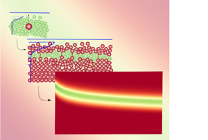
  $N_s = 1.5$. The bulk response of the granular mixture to this fluid forcing is represented by the dimensionless mixture streamwise velocity profile in figure 2(a). The inset is a semi-log plot of the dimensionless velocity profile and shows that it is exponential. As shown in figure 2(b), the linearity of the curve in the semi-log plot confirms that the shear rate is exponentially decreasing in the quasi-static part of the bed (delimited by the two horizontal black dashed lines). As expected for a uniform flow, the mixture shear stress
  $\tilde {\tau }_{xz}^m$ shown in figure 2(c) is linear with depth. For both quantities, the following fits were proposed and plotted as a red dotted line in figure 2:
 \begin{equation} \tilde{\dot{\gamma}}^m = \gamma_0 \,\textrm{e}^{\tilde{z}/s_0} \quad \text{and} \quad \tilde{\tau}^m_{xz} = a_0 \tilde{z} + \tau_0 .\end{equation}
The simulations performed by Chassagne et al. (Reference Chassagne, Maurin, Chauchat, Gray and Frey2020b) in this configuration were focused on the downward segregation of small particles. It was observed that the layer of small particles percolates rapidly for  $\tilde {z}> 8.5$ (flowing layer) and then slows down below (this limit is marked in figures 2(b) and 2(c)). Chassagne et al. (Reference Chassagne, Maurin, Chauchat, Gray and Frey2020b) showed that the small particles are advected downward like a travelling wave into the bed made of large particle with a layer of constant thickness. As figure 2(e) shows, the small particle concentration has a Gaussian-like shape and remains self-similar in time while segregating. The centre of mass of small particles,
  $\tilde {z}_c$, is therefore representative of the dynamics of the entire layer. Chassagne et al. (Reference Chassagne, Maurin, Chauchat, Gray and Frey2020b) observed that the small particle layer travels down as a logarithmic function of time
 \begin{equation} \tilde{z}_c(t) ={-}a_1 \ln \tilde{t} + b, \end{equation}
where  $a_1$ is a constant characterising the segregation velocity (
 $\textrm {d}\tilde {z}_c(t)/\textrm {d} \tilde {t} = - a_1/\tilde {t}$). The authors demonstrated that this logarithmic descent of small particles is a consequence of the dependency of the segregation velocity on the inertial number as
 \begin{equation} \dfrac{\textrm{d} \tilde{z}_c}{\textrm{d} t} \propto I^{0.85}(\tilde{z}_c). \end{equation}
Using (5.3) in the framework of the advection–diffusion model of Thornton et al. (Reference Thornton, Gray and Hogg2006) and Gray & Chugunov (Reference Gray and Chugunov2006) (see (1.5)) it was shown that the advection coefficient could be written as
 \begin{equation} S_{r} = S_{r0} I^{0.85}, \end{equation}
where  $S_{r0} = 0.049$, extending the inertial number dependency found by Fry et al. (Reference Fry, Umbanhowar, Ottino and Lueptow2018) to bi-disperse size segregation in the quasi-static regime. Then, with the help of a travelling wave method, they evidenced that the small particles percolate as a layer and with a self-similar concentration profile because the ratio between the advection coefficient and the diffusion coefficient is constant. The Péclet number reads
 \begin{equation} Pe = \dfrac{S_{r}}{D}, \end{equation}
and is therefore constant with  $\tilde {z}$, so that the diffusion coefficient has to have the same dependency on the inertial number as the segregation coefficient
 \begin{equation} D=D_{0} I^{0.85}, \end{equation}
where  $D_0$ is taken as
  $D_0 = 0.01$ and should be pressure independent (Fry et al. Reference Fry, Umbanhowar, Ottino and Lueptow2019).

Figure 2. Profiles and configuration from the DEM simulations. (a) Streamwise mixture velocity profile in the bed (——, blue solid line) and mixture volume fraction (——, green solid line). The inset is the semi-log plot of the velocity profile. (b) Solid shear rate (——, blue solid line) and the corresponding fit  $\tilde {\dot {\gamma }}^m = \gamma _0 \,\textrm {e}^{\tilde {z}/s_0}$ (- - - -, red dashed line) with
  $\gamma _0 = 1.64 \times 10^{-7}$ and
  $s_0 = 0.74$. (c) Solid shear stress and the corresponding fit
  $\tilde {\tau }_{xz}^m = a_0 \tilde {z} + \tau _0$ (- - - -, red dashed line) with
  $a_0=-0.078$ and
  $\tau _0=0.91$. The top and lower boundaries of the quasi-static bed are represented by (- - - -, black dashed lines). (d) Sketch of the numerical experiment with the input profiles for the rheology. (e) Concentration profile of small particles at the initial state for the multi-phase flow model (——, green solid line), the DEM (- - - -, black dashed line) and the mixture concentration profile
  $\phi$ (——, black solid line).
This work also demonstrated that the dynamics of the fine particle layer is controlled by its bottom position, which acts as a lower bound for the segregation velocity. In this way, the particles in the layer cannot segregate faster.
The numerical resolution of the 1-D multi-phase model a priori requires us to solve the granular rheology in order to estimate the granular viscosity required to evaluate the granular drag force contribution. The goal of the present study is to focus on grain-size segregation modelling. In addition, the results of Chassagne et al. (Reference Chassagne, Maurin, Chauchat, Gray and Frey2020b) were obtained in the quasi-static regime, for which there is still no consensus regarding granular rheology. For these reasons, the granular viscosity is directly determined by the DEM results here. This makes it possible to focus on the effect of the segregation model and to put aside potential discrepancies linked to a non-accurate description of the granular rheology. The friction coefficient is therefore computed from the DEM results using the definition
 \begin{equation} \mu = \dfrac{|\tau^m_{xz}|}{p^m}. \end{equation}
Similarly, the granular viscosity is computed using the definition
 \begin{equation} \eta^p = \dfrac{|\tau^m_{xz}|}{\left\vert \dot{\gamma^m_{xz}}\right\vert}. \end{equation}
As shown by the red dashed lines in figures 2(b) and 2(c), the fits presented in (5.1a,b) match the DEM results in the region  $8.5>\tilde {z}>3$. Thus, using these expressions in (5.8) provides an accurate estimate of the granular viscosity for the particle–particle drag closure. For this reason, the validation of the multi-phase flow model will only be carried out in this part of the bed. Therefore, the initial state consists in placing the small particles in the upper limit of the quasi-static part with the centre of mass
  $\tilde {z}^0_c = 8.5$. The sketch of this configuration is shown in figure 2(d). Figure 2(e) shows the small particle concentration profile of this numerical set-up at the initial state. The initial concentration is taken with a Gaussian fit on the DEM initial concentration (figure 2e), and ensures that the mass of particles is the same in the DEM and in the continuum simulations.
5.2. Comparison with the multi-phase flow model
The system of partial differential equations (3.8a,b)–(3.11) is solved numerically for the configuration shown in figure 2(d) with the initial concentration profile of figure 2(e). In these equations, the empirical segregation function is  $\mathcal {F}_l(\mu )$ and the drag coefficient
  $c$ is equal to 3, as suggested by Tripathi & Khakhar (Reference Tripathi and Khakhar2013). Because the fluid is incompressible, there is no equation of state for the fluid pressure. Nevertheless, remembering that
  $\epsilon +\varPhi =1$ and defining the volume-averaged velocities,
  $w = \epsilon w^f+ \varPhi w^m$, it can be demonstrated that the particle–fluid mixture is incompressible. A PISO (pressure implicit with splitting of operators) algorithm classically developed for thw incompressible Navier–Stokes equations is used to solve the pressure–velocity coupling. As the fluid pressure
  $p^f$ is the sum of the hydrostatic pressure and of the excess pore pressure
  $p^f = \overline {p^f} + \rho ^f g z$, the PISO algorithm consists in solving the momentum balance equations without
  $\overline {p^f}$ in a predictor step. Then, using the predicted velocity fields, a Poisson equation is solved to find
  $\overline {p^f}$. Once the pressure is found, the velocity fields are corrected. This kind of algorithm has already been used to model sediment transport in Chauchat et al. (Reference Chauchat, Cheng, Nagel, Bonamy and Hsu2017) and Chauchat (Reference Chauchat2018).
Figure 3 shows the results of the spatio-temporal evolution of the small particle concentration for the multi-phase flow model (figure 3a) and for the DEM (figure 3b). First, it can be seen that the dynamics predicted by the multi-phase flow model is similar to the DEM. The position of the bottom of the layer is approximately the same in both cases. More quantitatively, the centre of mass  $\tilde {z}_c$ of the small particle layer as a function of time is compared with the DEM in figure 4(a). After a first transient phase (
 $\tilde {t}>1\times 10^3$), the centre of mass position is linear in the semi-log plot, indicating that the logarithmic descent observed in the DEM simulation is well reproduced by the multi-phase flow model. The slope of the curve, representing coefficient
  $a_1$ of (5.2) is
  $0.68$ in the DEM simulation and
  $0.49$ for the multi-phase flow model, corresponding to an error of
  $28\,\%$. In addition, figure 4(b) shows that, in both models, the bottom of the layer is positioned at the same depth indicating that the multi-phase model reproduces well the bottom controlled behaviour observed by Chassagne et al. (Reference Chassagne, Maurin, Chauchat, Gray and Frey2020b) with DEM simulations. However, the Gaussian-like profile is not reproduced by the multi-phase flow model and a wider profile is obtained. In figure 3(a) the maximum concentration
  $\max (\phi ^s)$ (indicated by
  $\blacksquare$ in figure 4b) is almost two times smaller than the one predicted by the DEM simulation, while the extent of the small particle layer is much larger. These results indicate that, with the current parametrisation the multi-phase flow model is relevant to qualitatively predict the segregation dynamics. However, the error on the segregation velocity and the discrepancies on the concentration profile clearly show that the model needs to be improved.

Figure 3. Spatio-temporal plot of the small particle concentration in the bed obtained with (a) the multi-phase model, (b) the DEM simulation.

Figure 4. Results of the simulation for the multi-phase flow model (- $\cdot$-
 $\cdot$-, red dashed dot), the advection–diffusion model of (4.8) (——, green solid line) and the DEM (- - - -, black solid line). (a) Temporal evolution of the centre of mass. (b) Concentration profiles of small particles at the end of the simulation (
 $\tilde {t} \simeq 60\,000$);
  $\blacksquare$, represents the maximum concentration of the profiles.
5.3. Evaluation of the advection–diffusion model
In order to determine the ability of the advection–diffusion model to reproduce the same results as the multi-phase flow model, (4.8) is solved numerically. The resolution strategy is based on a conservative Godunov schemes where a no flux condition is applied at the bottom and on top of the vertical domain. A vertical discretisation of  $\textrm {d}\tilde {z} = h / 80$ is taken and the time step is computed in order to satisfy the Courant–Friedrichs–Lewy (CFL) condition. The initial solution is the same than in the multi-phase flow (figure 2e).
The numerical solution at time  $\tilde {t} = 60\,000$ is plotted in figure 4. Both the centre of mass (figure 4a) and the concentration profile (figure 4b) are almost superimposed with the multi-phase flow model solution, only slightly differing by numerical diffusion. Therefore, both models can be considered as strictly equivalent, meaning that the physical behaviour of the segregation forces added to the momentum equation of the small particles is accurately predicted by the single advection and diffusion coefficients of equation (4.8). Moreover, when deriving the advection–diffusion equation, it was assumed that the mixture volume fraction
  $\varPhi = cste$, the vertical acceleration of the small particles, the vertical mixture velocity and the fluid drag were negligible. The strong agreement between the models demonstrate that these assumptions are valid.
Equation (4.8) represents an important step in the upscaling since the behaviour of small particles can be predicted without solving the entire multi-phase flow model, providing a speed-up of one thousand for the numerical resolution of the equations. In the light of this result, the bi-disperse segregation problem can be simply viewed as a competition between the advection coefficient  $S_r$ and the diffusion coefficient
  $D$ of small particles. The interplay between both coefficients has been explored in more details by Fan et al. (Reference Fan, Schlick, Umbanhowar, Ottino and Lueptow2014b).
6. Discussion
The multi-phase flow model and the associated advection–diffusion model are able to reproduce qualitatively the DEM simulations and the main properties of segregation in bedload transport obtained by Chassagne et al. (Reference Chassagne, Maurin, Chauchat, Gray and Frey2020b) (bottom controlled segregation, logarithmic descent of the small particles). However, the segregation velocity is lower than in the DEM simulation and the shape of the small particle concentration profile is not adequately reproduced. So far, the inter-particle drag force and the segregation force from Guillard et al. (Reference Guillard, Forterre and Pouliquen2016) and Tripathi & Khakhar (Reference Tripathi and Khakhar2013) have not been modified. Guillard et al. (Reference Guillard, Forterre and Pouliquen2016) measured numerically the segregation force for a single intruder in a 2-D configuration and Tripathi & Khakhar (Reference Tripathi and Khakhar2013) developed their study in the context of density-driven segregation. These configurations are not general and the drag coefficient  $c$ as well as the empirical segregation function
  $\mathcal {F}_l(\mu )$ are expected to be different when considering an ensemble of particles since there could be some collaborative effects that are not taken into account in these forces. Therefore, in § 6.1, a sensitivity analysis to the empirical segregation function is presented. Then, in § 6.2, new formulations of the empirical segregation function
  $\mathcal {F}_l(\mu )$ and of the drag coefficient
  $c$ will be proposed based on the DEM results.
As the advection–diffusion equation results are strictly identical with the multi-phase flow equations, the discussion and the associated simulations will only be performed with the advection–diffusion equation.
6.1. Investigation of the empirical segregation function  $\mathcal {F}_l$

Numerical data from Guillard et al. (Reference Guillard, Forterre and Pouliquen2016) for the empirical segregation function  $\mathcal {F}_l(\mu )$ exhibit a significant scatter and it is possible to show that a constant function could also fit the data (see Appendix A). In this section, an analysis of the sensitivity to the empirical segregation function, taken as constant and varying from
  $\mathcal {F}_l = 1$ to
  $\mathcal {F}_l = 15$, is presented.
Figure 5(a) shows the temporal evolution of the small particle centre of mass for the different values of the empirical segregation function  $\mathcal {F}_l$. The linear evolution in the semi-logarithmic plot is conserved with the same slope (coefficient
  $a_1$ in (5.2)), whatever the value of the empirical segregation function, meaning that the segregation velocity
  $\textrm {d}\tilde {z}_c / \textrm {d}\tilde {t}$ is not modified when changing the empirical segregation function. Increasing
  $\mathcal {F}_l$ only makes the curves shift vertically. Figure 5(b) shows that the maximum concentration is better predicted when increasing the empirical segregation function. On reaching
  $\mathcal {F}_l = 15$, agreement with DEM results is perfect. The previous simulation, where the empirical segregation function
  $\mathcal {F}_l$ is a function of the friction coefficient
  $\mu$, is also plotted in this figure. It is interesting to note that simulation with
  $\mathcal {F}_l = 1$ is almost superimposed with the one obtained with
  $\mathcal {F}_l(\mu )$. These observations tend to show that the friction coefficient dependency has a small influence on the size segregation configuration investigated. Therefore, taking
  $\mathcal {F}_l$ as constant is a good approximation, at first order.

Figure 5. Comparison with the DEM (- - - -, black dashed line) for various values of  $\mathcal {F}_l = cste$ for the temporal evolution of (a) the centre of mass and (b) the maximum concentration of
  $\phi ^s$.
Chassagne et al. (Reference Chassagne, Maurin, Chauchat, Gray and Frey2020b) showed that the advection coefficient  $S_r$ was a function of the inertial number
  $I$ (see (5.4)) and linked the logarithmic descent to the exponential form of
  $I$ in
  $S_r$. In the proposed model, the advection coefficient
  $S_r = \mathcal {F}_l St^p \partial \tilde {p}^m / \partial \tilde {z}$ (4.9a,b). In this coefficient, since the solid pressure gradient is constant in the bed (4.2a,b) and
  $\mathcal {F}_l = cste$, there is only one non-constant variable which is the inverse of the granular viscosity
  $1/\eta ^p$ appearing in the granular Stokes number (2.9). As figure 5(a) shows that the logarithmic descent is still preserved with this parametrisation, this demonstrates that the viscosity profile is mainly responsible for the logarithmic descent. Therefore, in the proposed advection coefficient
  $S_r$, the empirical segregation function
  $\mathcal {F}_l$ controls the strength of the segregation force and can be seen as a forcing parameter. In contrast, the velocity at which the small grains are descending is controlled by the granular viscosity in the granular Stokes number
  $St^p$. In this way, the segregation problem can simply be seen as the settling of small particles under a force proportional to the empirical segregation function
  $\mathcal {F}_l$, into a complex fluid having a variable viscosity.
It should be noted that there is a direct relation between the dimensionless granular viscosity and the inertial number (see Appendix B) written
 \begin{equation} I = \dfrac{\mu \sqrt{\tilde{p}^m}}{\widetilde{\eta^p}}, \end{equation}
where  $\tilde {\eta }^p = \eta ^p / \rho ^p d_l W$ is the dimensionless granular viscosity and
  $\mu = \vert \tilde {\tau }_{xz}^m\vert / \tilde {p}^m$ is the friction coefficient. Since the variation of
  $\mu$ and
  $\sqrt {\tilde {p}^m}$ is small compared with the exponential profile of
  $\tilde {\eta }^p$, the inversely proportional relation between the granular viscosity and the inertial number shows that the inertial number dependency found by Chassagne et al. (Reference Chassagne, Maurin, Chauchat, Gray and Frey2020b) can be seen as a dependency on the inverse granular viscosity, confirming the important role of the granular viscosity in the segregation dynamics.
Figure 5(b) showed that a better maximum concentration was predicted with  $\mathcal {F}_l = 15$. However, the value of the empirical segregation function
  $\mathcal {F}_l$ should have no influence on the diffusion as
  $D = \phi ^s / \varPhi \tilde {p}^m St^p$. This influence can be explained by the Péclet number
  $Pe =S_r/D$. Indeed, when
  $\mathcal {F}_l$ increases, the advection coefficient
  $S_r$ increases as well and makes the Péclet number higher. As a result, the diffusive effect becomes small compared with the advection and, thus, the small particles stay more concentrated. However, the dynamics of the centre of mass shows a better agreement for
  $\mathcal {F}_l=1$ (see figure 5a) than for
  $\mathcal {F}_l = 15$, meaning that the diffusion coefficient needs to be improved.
The advection coefficient  $S_r$ and the diffusion coefficient
  $D$ have been plotted in figures 6(a) and 6(b) with
  $\mathcal {F}_l = 1$, for
  $\phi ^s = \max (\phi ^s)$. For
  $\tilde {z} > 7$,
  $S_r$ is close to the values predicted by the DEM. Under this limit, both curves are exponentially decreasing into the bed but with a different slope, leading to discrepancies. This shows that the
  $1/\eta ^p$ dependency has a fundamental role in the vertical structure of the advection coefficient
  $S_r$. Yet, another dependency with depth is probably missing in the empirical segregation function or in the drag coefficient
  $c$ to find again a similar slope to the DEM. Surprisingly, the proposed diffusion coefficient has the same slope as the one predicted by the DEM, which means that it contains the correct depth dependency. However, its value is too high by a factor ten, explaining why the advection–diffusion results are too diffusive.

Figure 6. (a) Advection coefficient in the bed (4.8) with  $\mathcal {F}_l = 1$, for
  $N_s = 1.5$ (—–, blue solid line) and
  $S_{r0} I^{0.85}$ proposed by Chassagne et al. (Reference Chassagne, Maurin, Chauchat, Gray and Frey2020b) (- - - -, black dashed line). (b) Diffusion coefficient in the bed from (4.8) for
  $\phi ^s = \max (\phi ^s)$ for the case
  $N_s=1.5$ (—–, blue solid line) and
  $D_0 I^{0.85}$ proposed by Chassagne et al. (Reference Chassagne, Maurin, Chauchat, Gray and Frey2020b) (- - - -, black dashed line).
6.2. Missing dependencies in the particle-scale forces
In the present paper, the advection and diffusion coefficients (4.9a,b) have been derived from particle-scale segregation and solid drag forces of Guillard et al. (Reference Guillard, Forterre and Pouliquen2016) and Tripathi & Khakhar (Reference Tripathi and Khakhar2013). However, figure 6 shows that both coefficients should be improved so as to match the DEM results. The segregation and solid drag forces of Guillard et al. (Reference Guillard, Forterre and Pouliquen2016) and Tripathi & Khakhar (Reference Tripathi and Khakhar2013) have been established in idealised granular segregation configurations (e.g. unique intruder, simple forcing, 2-D DEM) so that one can expect the two formulations to miss some dependencies when considering more general cases (mixture of small and large particles, 3-D modelling or complex forcing). Such dependencies probably lie in the drag coefficient  $c$ and the empirical segregation function
  $\mathcal {F}_l$ contained in the advection and diffusion coefficients. While the drag coefficient
  $c$ was taken as constant in their study, Tripathi & Khakhar (Reference Tripathi and Khakhar2013) and Duan et al. (Reference Duan, Umbanhowar, Ottino and Lueptow2020) suggested that it could depend on the local concentration of particles. Similarly to a hindrance function in a fluid flow, one indeed expects an increase of the effective solid drag force on a particle with increasing concentration. This dependency of the drag coefficient in the local particle concentration should also impact the diffusion coefficient profile (see figure 6b) and makes it possible to match the DEM. In addition, to correct the slope of the advection coefficient
  $S_r$ (see figure 6a), only the empirical segregation function
  $\mathcal {F}_l$ should vary with depth.
As detailed in § 5.1, Chassagne et al. (Reference Chassagne, Maurin, Chauchat, Gray and Frey2020b) have been able to express the advection and diffusion coefficient dependencies on the inertial number  $I$ (see (5.4) and (5.6)). In the following, both DEM and advection–diffusion coefficients are compared so as to extract the potential missing dependencies of
  $\mathcal {F}_l$ and
  $c$ from the DEM coefficients and to propose new formulations of these parameters. Then, it is verified that the results from the advection–diffusion model are consistent when using these proposed closures.
In order to compare the advection and diffusion coefficients to the DEM and to find the missing dependencies, it is first shown that the coefficients of equation (4.9a,b) can be expressed with an inertial number dependency as in the DEM. Indeed, as already shown in (6.1), the granular Stokes number can be rewritten as a function of the inertial number  $I$
$I$
 \begin{equation} St^p = \dfrac{I}{6c \mu \sqrt{\tilde{p}^m}}. \end{equation}
With this new definition, the advection and diffusion coefficients obtained in (4.9a,b) can be rewritten as a function of the inertial number  $I$
$I$
 \begin{equation} S_r = \dfrac{I \mathcal{F}_l}{6 c \mu \sqrt{\tilde{p}^m}} \displaystyle\frac{\partial\tilde{p}^m}{\partial\tilde{z}} \quad \text{and} \quad D = \dfrac{ \phi^s \sqrt{\tilde{p}^m} I}{\varPhi 6 c \mu}. \end{equation}
One can notice that  $\sqrt {\tilde {p}^m} I = \tilde {\dot {\gamma }}$, which makes the diffusion coefficient directly proportional to the shear rate. Such a dependency for the diffusion coefficient was found in a size bi-disperse case by Cai et al. (Reference Cai, Xiao, Zheng and Zhao2019) and Fry et al. (Reference Fry, Umbanhowar, Ottino and Lueptow2019) with DEM simulations. This shows that the particle–particle force-based model is able to explain a dependency found in different experiments. It represents a powerful argument to show the robustness of the proposed model. Yet, the power
  $0.85$ highlighted by the DEM does not seem to appear. In figure 7 the profile of
  $\sqrt {\tilde {p}^m} I / \mu$, the profiles of
  $I^{0.85}$ from the DEM and from exponential fitting are plotted. One can observe that values only differ by a factor
  $D_0^{\prime } / I_0^{\prime } = 1.13$ and that the exponential evolution with depth is the same, which proves that, in this case,
 \begin{equation} \dfrac{\sqrt{\widetilde{p^m}} I}{\mu} \propto I^{0.85}. \end{equation}
Such a result shows that the diffusion coefficient of the proposed model (6.3a,b) has the same dependency with  $I^{0.85}$ as the diffusion coefficient proposed by Chassagne et al. (Reference Chassagne, Maurin, Chauchat, Gray and Frey2020b). This explains the identical evolution with depth between both coefficients in figure 6(b), and shows that the advection equation and the multi-phase flow model are physically consistent.

Figure 7. Value of  $I^{0.85}$ computed from DEM results (——, black solid line) and its exponential fit
  $I_0^{\prime } e^{\tilde {z}/s_2}$ (- - - -, red dashed line) compared to
  $\sqrt {\tilde {p}^m} I / \mu$ (——, yellow solid line) and its exponential fit
  $D_0^{\prime } \,\textrm {e}^{\tilde {z}/s_3}$ (- - - -, black dashed line);
  $I_0^{\prime } = 7.52 \times 10^{-7}$,
  $s_2 = 0.8$,
  $D_0^{\prime } = 8.46 \times 10^{-7}$ and
  $s_3 = 0.78$.
Assuming that the drag coefficient includes the accurate dependencies, the following equality should be obtained between diffusion coefficients of the DEM and the one proposed in (6.3a,b):
 \begin{equation} \dfrac{\phi^s \sqrt{\widetilde{p^m}} I}{\varPhi 6 c \mu} = D_0I^{0.85}. \end{equation}
As demonstrated in (6.4),  $\sqrt {\tilde {p}^m} I / \mu I^{0.85} = C_0$, where
  $C_0$ is a constant (see Appendix C for the details) the drag coefficient
  $c$ can be deduced from (6.5):
 \begin{equation} c(\phi^s) = \dfrac{C_0}{6\varPhi D_0} \phi^s = 31 \phi^s. \end{equation}
As a consequence of this linear scaling in concentration, the dependency on the small particle volume fraction vanishes in the diffusion coefficient (4.9a,b). This modification will tend to smooth out the small particle concentration profile. In this drag coefficient, when  $\phi ^s \rightarrow 0$ (i.e. one small particle in a bath of large particles), the drag coefficient vanishes while it should reach a constant value,
  $c=3$ as shown by Tripathi & Khakhar (Reference Tripathi and Khakhar2013). To ensure a consistent formulation, it is therefore proposed that
  $c(\phi ^s)$ reads
 \begin{equation} c(\phi^s) = 3\left(1+\frac{28}{3}\phi^s\right), \end{equation}
which tends to  $3$ when
  $\phi ^s \rightarrow 0$ and to
  $31$ when
  $\phi ^s \rightarrow 1$.
As mentioned in the last section, the empirical segregation function  $\mathcal {F}_l$ is expected to depend on depth (see figure 6a). In this way, the advection coefficient should correspond to the DEM and it follows
 \begin{equation} \dfrac{I \mathcal{F}_l}{6 c(\phi^s) \mu \sqrt{\tilde{p}^m}} \left\vert\displaystyle\frac{\partial\tilde{p}^m}{\partial\tilde{z}}\right\vert =S_{r0}I^{0.85}. \end{equation}
From this equation and using (6.4), one can express the empirical segregation function, for  $\rho ^p \ne \rho ^f$, as
 \begin{equation} \mathcal{F}_l(\tilde{p}^m, \phi^s) = \mathcal{F}_0 c(\phi^s) \tilde{p}^m, \end{equation}
where  $\mathcal {F}_0 = 6 S_{r0} \rho ^p / (C_0 \varPhi (\rho ^p - \rho ^f))$. This result is the consequence of the scaling obtained for the advection coefficient in the DEM simulation. In the latter, only the local solid volume fraction
  $\phi ^s$ and the pressure
  $\tilde {p}^m$ are varying. Other dependencies can therefore be contained in
  $S_{r0}$ and should not be interpreted. Focusing on the meaningful terms, the empirical segregation function is logically found to depend on the small particle concentration, as expected when considering a mixture of particles. The pressure dependency suggests that the segregation function could depend on the stress state and that the local pressure could drive the lift force. Guillard et al. (Reference Guillard, Forterre and Pouliquen2014) found the lift force to increase with depth until a saturation depth where this force becomes constant. The pressure dependency found in (6.9) could explain the increasing lift force with depth and imply that in the studied configuration the saturation depth is not reached.
With the new formulations of the solid drag coefficient  $c(\phi ^s)$ and the empirical segregation function
  $\mathcal {F}_l(\tilde {p}^m, \phi ^s)$, it is verified that the DEM results can be reproduced. This is done with simulations accounting for different initial quantities of small particles (
 $N_s = {0.5, 1, 1.5, 2}$). Figure 8 shows the results for the time evolution of the centre of mass and the final concentration profile. Both the mass centres and the final concentration profiles are fairly well superimposed with the DEM results. Therefore, the new parametrisation is consistent with the DEM simulations. The concentration profile with the original parametrisations of
  $c$ and
  $\mathcal {F}_l(\mu )$ (see figure 4b) has also been plotted in figure 8 (
 $N_s=1.5$). The shape of the final concentration profile has drastically changed, from a bell shape to the expected Gaussian-like shape. This is attributed to the small particle concentration dependency in the drag coefficient, which cancels the original concentration dependency in the diffusion coefficient.

Figure 8. (a–d) Temporal evolution of the centre of mass for  $N_s = {0.5, 1, 1.5, 2}$. (e–h) Final small particle concentration profile for
  $N_s = {0.5, 1, 1.5, 2}$. In the panels, (- - - -, black dashed line) are the DEM results from Chassagne et al. (Reference Chassagne, Maurin, Chauchat, Gray and Frey2020b). The concentration profile obtained without any parametrisation, in the case
  $N_s = 1.5$ (from figure 4b), has also been plotted (
 $\cdots \cdots \cdot$).
Lastly, note that changing the parametrisation of the forces still yields physical solutions which proves that the advection–diffusion model and the corresponding multi-phase flow model are physically consistent and robust.
6.3. Influence of the size ratio
Guillard et al. (Reference Guillard, Forterre and Pouliquen2016) and Jing et al. (Reference Jing, Ottino, Lueptow and Umbanhowar2020) showed that the segregation force depends on the size ratio  $r = d_l / d_s$ and exhibits a maximum for a size ratio of
  $r = 2$. Schlick et al. (Reference Schlick, Fan, Isner, Umbanhowar, Ottino and Lueptow2015) found the segregation velocity of an ensemble of small particles to be dependent on the logarithm of the size ratio for
  $r<3$ and also found the segregation velocity to reach its maximum for
  $r \sim 2$. Based on DEM simulations, Chassagne et al. (Reference Chassagne, Maurin, Chauchat, Gray and Frey2020b) also studied the size-ratio dependency. Surprisingly, it was found that the segregation velocity of the percolating small particles was a monotonic increasing function of
  $r$. Best fit of the DEM results suggested the following dependency
  $f(r) = 0.45(\exp ({(r-1)/1.59}-1))$ for the advection coefficient
  $S_r$. Further studies on the effect of the size ratio on segregation are needed to explain the difference between the studies of Golick & Daniels (Reference Golick and Daniels2009), Schlick et al. (Reference Schlick, Fan, Isner, Umbanhowar, Ottino and Lueptow2015) and Guillard et al. (Reference Guillard, Forterre and Pouliquen2016). A potential reason could lie in the configuration difference. For example, it could shift the value of the maximum segregation efficiency to higher values of
  $r$ that have not been investigated by Chassagne et al. (Reference Chassagne, Maurin, Chauchat, Gray and Frey2020b).
This dependency is introduced into the empirical segregation function  $\mathcal {F}_l$ as follows:
 \begin{equation} \mathcal{F}_l(\tilde{p}^m, \phi^s, r) = \mathcal{F}_0 f(r) c(\phi^s)\tilde{p}^m. \end{equation}
Using this parametrisation, simulations have been performed for  $r=1.25, 1.5, 1.75, 2, 2.25$. The results are plotted in figure 9 and compared with DEM simulations. For each case, the centre of mass position is in very good agreement with the DEM simulations. For the lower size ratio, the concentration profiles are superimposed with the DEM results while for the higher size ratios (
 $r=2$ and
  $r = 2.25$) the maximum concentrations are slightly higher than the DEM. This indicates that the model is not diffusive enough. Indeed, the size-ratio dependency has only been introduced in the advection coefficient. As shown in § 6.1, the shape of the concentration profile results from a subtle balance between advection and diffusion through the Péclet number,
  $Pe$. For the highest size ratio, this balance is not perfectly reproduced by the proposed model, which indicates that the diffusion coefficient should also depend on the size ratio. This would imply that the granular Stokes number also depends on the size ratio. It could explain why Guillard et al. (Reference Guillard, Forterre and Pouliquen2016) found a maximum segregation force for a size ratio
  $r=2$, while Chassagne et al. (Reference Chassagne, Maurin, Chauchat, Gray and Frey2020b) found the advection coefficient
  $S_r$ to increase exponentially with the size ratio. Further research is needed to elucidate this point through a detailed investigation of the granular Stokes number dependency on the size ratio.

Figure 9. (a–e) Temporal evolution of the centre of mass for  $N_s = 1$ and
  $r = {1.25, 1.5, 1.75, 2, 2.25}$. (f–j) Final small particle concentration profile for
  $N_s = 1$ and
  $r = {1.25, 1.5, 1.75, 2, 2.25}$. In these panels, (——, black solid line) corresponds to the advection–diffusion model and (- - - -, black dashed line) are the DEM results from Chassagne et al. (Reference Chassagne, Maurin, Chauchat, Gray and Frey2020b).
7. Conclusion
In this contribution, size segregation in bi-disperse systems has been investigated with a special focus on bedload transport. The originality of the work presented herein is to propose a new multi-phase flow approach, derived from a volume-averaging technique, based on the most recent advances in particle–particle forces, namely the segregation force or lift force from Guillard et al. (Reference Guillard, Forterre and Pouliquen2016) and the drag force from Tripathi & Khakhar (Reference Tripathi and Khakhar2013). The proposed multi-phase flow model formulation is very general and it can be applied to any immersed granular flow configuration. In a subsequent step, following the same procedure as in Thornton et al. (Reference Thornton, Gray and Hogg2006), an advection–diffusion model is derived from the multi-phase flow equations. This derivation allows us to identify the dependencies of the advection and diffusion coefficients on the local physical parameters of the flow such as the volume fraction of small particles, the mixture granular pressure and its gradient, the granular Stokes number and the segregation parameter.
Both models have been tested against the DEM simulations of Chassagne et al. (Reference Chassagne, Maurin, Chauchat, Gray and Frey2020b) for bi-disperse turbulent bedload transport. Without any tuning of the forces from Guillard et al. (Reference Guillard, Forterre and Pouliquen2016) and Tripathi & Khakhar (Reference Tripathi and Khakhar2013), both continuum models qualitatively reproduce the main features of size segregation. This demonstrates that the scaling of the advection coefficient with the inertial number observed by Fry et al. (Reference Fry, Umbanhowar, Ottino and Lueptow2018) and Chassagne et al. (Reference Chassagne, Maurin, Chauchat, Gray and Frey2020b) can be explained thanks to the dependency of the advection coefficient on the granular Stokes number and the underlying presence of the granular viscosity. Using the discrete element simulation results, improved parametrisations for the advection and diffusion coefficients have been proposed. They suggest that the empirical segregation function from Guillard et al. (Reference Guillard, Forterre and Pouliquen2016) and the drag coefficient from Tripathi & Khakhar (Reference Tripathi and Khakhar2013) should incorporate a dependency on the small particle concentration. At last, the influence of the size ratio has been investigated and a dependency of the segregation function on the size ratio has been proposed.
In terms of perspectives for granular flows, the continuum models proposed herein are very general and should also apply to dense dry granular flows. These models represent a general framework for developing and testing improved parametrisations for the segregation and granular drag forces in different flow configurations. Further work is needed to identify and propose more robust concentration, depth and size-ratio dependencies of the empirical dimensionless coefficients appearing in both granular forces. Concerning the upscaling of size segregation processes in sediment transport applications, two routes are opened. The first one consists in implementing the proposed multi-phase flow model in a 3-D numerical model, such as sedFOAM (Chauchat et al. Reference Chauchat, Cheng, Nagel, Bonamy and Hsu2017), for the simulation of size segregation in complex sediment transport applications such as riverbed armouring (Frey & Church Reference Frey and Church2009), scour around an hydraulic structure (Nagel et al. Reference Nagel, Chauchat, Bonamy, Liu, Cheng and Hsu2020) or wave-driven sediment transport involving sand mixtures (O'Donoghue & Wright Reference O'Donoghue and Wright2004). The second route would be to couple the advection–diffusion model with a shallow water model for the fluid flow. Such a model would make it possible to address size segregation at larger scales while taking into account granular-scale processes in a physically consistent way (Woodhouse et al. Reference Woodhouse, Thornton, Johnson, Kokelaar and Gray2012; Denissen et al. Reference Denissen, Weinhart, Te Voortwis, Luding, Gray and Thornton2019).
Funding
This research was funded by the French Agence nationale de la recherche, project ANR-16-CE01-0005 SegSed ‘size segregation in sediment transport’. The authors acknowledge the support of Irstea (now INRAE, formerly Cemagref). INRAE, ETNA is member of Labex TEC21 (Investissements d'Avenir Grant Agreement ANR-11-LABX-0030) and Labex Osug@2020 (Investissements d'enir Grant Agreement ANR-10-LABX-0056).
Declaration of interests
The authors report no conflict of interest.
Appendix A. New formulation of $\mathcal {F(\mu )}$ for a single large particle

In this part, it is shown that the empirical function  $\mathcal {F}(\mu )$ of (1.3a,b) does not make it possible to define the total segregation force as a sum of the granular buoyancy and the granular lift force. Therefore, a new formulation is proposed.
Considering an immobile bed, segregation should stop and therefore  $w^l = 0$. In this case, the drag forces vanish and the friction coefficient should be equal to the static friction coefficient
  $\mu = \mu _c$. Therefore, the segregation force of (1.2) counter-balances the weight of the particle as
 \begin{equation} \left(\rho^p-\rho^f\right)g \cos \theta+ \mathcal{F}(\mu_c) \displaystyle\frac{\partial p^s}{\partial\tilde{z}} =0. \end{equation}
For a dense flow with small velocity fluctuations, the small particle pressure is the lithostatic pressure  $p^s = \varPhi _{max} (\rho ^p - \rho ^f) g \cos \theta (h-z)$. The particle pressure gradient is therefore
  $\partial p^s /\partial z = - \varPhi _{max} (\rho ^p - \rho ^f) g \cos \theta$. Introducing this expression in (A1), it finally imposes that
 \begin{equation} \mathcal{F}(\mu_c) = \dfrac{1}{\varPhi_{max}}. \end{equation}
The condition (A2) shows that the segregation force should balance the hydrostatic particle pressure, at rest. However, the functional form (1.3a,b) proposed by Guillard et al. (Reference Guillard, Forterre and Pouliquen2016) and plotted in figure 10, does not satisfy condition (A2) in the quasi-static regime ( $\mu <0.3$). In order to verify condition (A2), the following form is proposed:
 \begin{equation} \mathcal{F}(\mu) = \dfrac{1}{\varPhi_{max}} + \mathcal{F}_l(\mu), \end{equation}
with  $\mathcal {F}_{l}(\mu ) = (1-\exp ({-70(\mu -\mu _c)}))$. Equation (A3) is plotted in figure 10. It can be observed that it is close to (1.3a,b) for
  $\mu \gg \mu _c$ but decreases to
  $1/\varPhi _{max}$ in the static regime. This makes it possible to write the segregation force as
 \begin{equation} f_{seg} = V_l \left(\dfrac{1}{\varPhi_{max}} + \mathcal{F}_{l}(\mu)\right) \displaystyle\frac{\partial p^s}{\partial z} , \end{equation}
where  $\varPi _p = V_l / \varPhi _{max} \partial p^s/\partial z$ is the granular buoyancy force and
  $f_l = V_l \mathcal {F}_l(\mu ) \partial p^s/\partial z$ is the granular lift force.

Figure 10. Empirical segregation function  $\mathcal {F}(\mu )$ of the segregation force
  $f_{seg} = V_l \mathcal {F}(\mu ) \partial p^s / \partial z$ found by Guillard et al. (Reference Guillard, Forterre and Pouliquen2016) as a function of the local friction coefficient
  $\mu$. Here,
  $+$ are the simulation results found by Guillard et al. (Reference Guillard, Forterre and Pouliquen2016) using DEM, (——, red solid line) is the function they proposed and (——, blue solid line) is
  $\mathcal {F}(\mu ) = 1 / \varPhi + (1-\exp ({-70(\mu -\mu _c)}))$, the improved function proposed.
Appendix B. Link between the viscosity $\eta ^p$ and the inertial number $I$


The inertial number of large particles is
 \begin{equation} I = \dfrac{\dot{\gamma}^m d_l}{\sqrt{p^m / \rho^p}}. \end{equation}
Considering that
 \begin{equation} \eta^p = \dfrac{\vert\tau^m_{xz}\vert}{\vert\dot{\gamma}^m\vert} \quad \text{and} \quad \tau^m_{xz} = \mu p^m, \end{equation}
the inertial number can be written as
 \begin{equation} I = \dfrac{\mu d_l \sqrt{p^m \rho^p}}{\eta^p}. \end{equation}
Then, making  $\eta ^p$ dimensionless with the scaling
  $\rho ^p d_l W$, one can obtain
 \begin{equation} I = \dfrac{\mu \sqrt{\tilde{p}^m}}{\tilde{\eta^p}}. \end{equation}
Appendix C. Deriving of the parameters $\mathcal {F}_l$ and $c$ using DEM results


In this appendix, the methods to derive the advection and diffusion coefficients from the DEM simulations are developed. For the diffusion coefficient, this consists in proposing a new formulation of the drag coefficient, based on the small particle concentration, to found the accurate values of the diffusion coefficient. For the advection coefficient, it consists in rewriting the empirical segregation function  $\mathcal {F}_l$, in order to find the same dependency with depth as the advection coefficient from the DEM simulations.
C.1. New formulation of the drag coefficient $c$

In this part, the idea is to propose a new drag coefficient  $c$ that satisfies
 \begin{equation} \dfrac{ \phi^s \sqrt{\tilde{p}^m} I}{\varPhi 6 c \mu} = D_0I^{0.85}. \end{equation}
Since it was found that
 \begin{equation} \displaystyle \dfrac{\sqrt{\tilde{p}^m} I}{\mu} = D_0^{\prime} \,\textrm{e}^{\tilde{z}/s_3} \quad \text{with} \ D_0^{\prime} = 8.46 \times 10^{{-}7} \quad s_3 = 0.78, \end{equation}
and
 \begin{equation} \displaystyle I^{0.85} = I_0^{\prime} \,\textrm{e}^{\tilde{z}/s_2} \quad \text{with} \ I_0^{\prime} = 7.52 \times 10^{{-}7} \quad s_2 = 0.8, \end{equation}
it can be written that
 \begin{equation} \dfrac{\sqrt{\tilde{p}^m} I}{ \mu I^{0.85}} = \dfrac{D_0^{\prime}}{I_0^{\prime}} = C_0, \end{equation}
where  $C_0 = 1.13$. In this way, (C1) becomes
 \begin{equation} c(\phi^s) = \phi^s \dfrac{C_0}{6 \varPhi D_0} = 31 \phi^s. \end{equation}
C.2. New formulation of the empirical segregation function $\mathcal {F}_l$

The new empirical segregation function has to fill the gap with the advection coefficient found using DEM. Therefore,  $\mathcal {F}_l$ is such that
 \begin{equation} \dfrac{I \mathcal{F}_l}{6 c(\phi^s) \mu \sqrt{\tilde{p}^m}} \left\vert\displaystyle\frac{\partial\tilde{p}^m}{\partial\tilde{z}}\right\vert =S_{r0}I^{0.85}. \end{equation}
In (C6), the dimensionless pressure gradient is constant and, using the hydrostatic approximation with  $\cos \theta \sim 1$, reads
 \begin{equation} \partial \tilde{p}^m/ \partial \tilde{z} ={-} \varPhi \left(\rho^p - \rho^f\right) / \rho^p. \end{equation}
Introducing it in (C6) and remembering that  $\sqrt {\tilde {p}^m} I / \mu I^{0.85} = C_0$, the empirical segregation function must satisfy
 \begin{equation} \mathcal{F}_l(\tilde{p}^m, \phi^s) = \dfrac{6 S_{r0} \rho^p}{C_0 \varPhi (\rho^p - \rho^f)}c(\phi^s)\tilde{p}^m . \end{equation}


