


1. Introduction
Internally heated (IH) convection, in which the motion of a fluid is driven by buoyancy forces caused by internal sources of heat, is found in a wide variety of natural and built environments, and plays an essential role in disciplines such as geophysics and astrophysics. For example, radioactive decay drives convection in the Earth's mantle, which in turn influences plate tectonics and the planet's magnetic field (Bercovici Reference Bercovici2011). A similar mechanism explains geological patterns on the surface of Pluto (Trowbridge et al. Reference Trowbridge, Melosh, Steckloff and Freed2016), and buoyancy driven flows due to the absorption of solar radiation induces atmospheric turbulence on Venus (Tritton Reference Tritton1975).
Internal heating generalises thermal forcing at the boundaries typical of Rayleigh– Bénard models of convection in both a theoretical and a practical sense, because internal heat sources can be concentrated near boundaries to produce the latter (Bouillaut et al. Reference Bouillaut, Lepot, Aumaître and Gallet2019). The dynamics of IH convection is also closely related, and sometimes equivalent, to that of flows driven by internal sources of buoyancy besides temperature, such as density stratification due to electromagnetic forces or chemical concentration differences (Goluskin Reference Goluskin2016). IH convection therefore warrants study in its own right to enhance fundamental understanding of buoyancy-driven turbulence, yet has received relatively little attention in comparison with Rayleigh–Bénard convection.
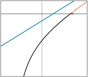
A fundamental challenge in the study of IH convection, along with many other turbulent flows, is to characterise the flow's statistical properties as a function of its control parameters. Following previous work (Goluskin & Spiegel Reference Goluskin and Spiegel2012; Goluskin Reference Goluskin2016), we consider this problem in the idealised configuration illustrated in figure 1, where a horizontal layer of fluid between isothermal plates of equal temperature is heated uniformly at a constant rate. The only control parameters for this setting are the Prandtl number of the fluid, Pr, and the Rayleigh number based on the internal heating rate, R. Particular statistical quantities of interest are the dimensionless mean temperature,  $\langle T \rangle$, and the dimensionless mean vertical convective heat flux,
  $\langle wT \rangle$, where the mean is obtained by averaging over volume and infinite time and w is the component of the velocity in the vertical direction.

Figure 1. Schematic diagram for convection driven by unit uniform internal heat generation (IH) between two isothermal parallel plates. The averaged heat fluxes through the top and bottom plates are denoted by  $\mathcal {F}_1$ and
  $\mathcal {F}_0$, respectively. Red lines illustrate the temperature profile in the conductive regime (- - -, red dashed) and a typical mean temperature profile in the turbulent regime (—, red solid line).
The dimensionless mean temperature  $\langle T\rangle$ corresponds to the amount of thermal dissipation in the fluid and can be related qualitatively to the proportion of heat within the fluid that is transported by conduction, rather than by convection. As described by Goluskin & Spiegel (Reference Goluskin and Spiegel2012, p. 87), the average outward conduction above and below the plane over which the time- and plane-averaged temperature
  $\bar {T}$ is maximised is equal to
  $2\bar {T}$. If one assumes that at high R the temperature field is well mixed, then
  $\langle T\rangle$ scales in the same way as the maximum of
  $\bar {T}$. The ratio of the total (predominantly convective) heat flux to the conductive heat flux, which corresponds to a Nusselt number, is therefore
  $1/(2\bar {T}) \sim 1/\langle T\rangle$. In contrast,
  $\langle wT\rangle$ quantifies the vertical asymmetry caused by the fluid's motion and is related to the heat fluxes
  $\mathcal {F}_1$ and
  $\mathcal {F}_0$ through the top and bottom boundaries by the exact relations (Goluskin Reference Goluskin2016)
 \begin{equation} \mathcal{F}_1 = \tfrac12 + \langle wT \rangle, \quad \mathcal{F}_0 = \tfrac12 - \langle wT \rangle. \end{equation}
 Laboratory experiments (Kulacki & Goldstein Reference Kulacki and Goldstein1972; Jahn & Reineke Reference Jahn and Reineke1974; Mayinger et al. Reference Mayinger, Jahn, Reineke and Steibnberner1976; Kakac, Aung & Viskanta Reference Kakac, Aung and Viskanta1985; Lee, Lee & Suh Reference Lee, Lee and Suh2007) and direct numerical simulations (Peckover & Hutchinson Reference Peckover and Hutchinson1974; Straus Reference Straus1976; Tveitereid Reference Tveitereid1978; Emara & Kulacki Reference Emara and Kulacki1980; Wörner, Schmidt & Grötzbach Reference Wörner, Schmidt and Grötzbach1997; Goluskin & Spiegel Reference Goluskin and Spiegel2012; Goluskin & van der Poel Reference Goluskin and van der Poel2016) indicate that the dimensional mean temperature increases sublinearly with the heating rate, which, in non-dimensional terms, implies that  $\langle T \rangle$ decreases with
  ${\textit {R}}$. Scaling arguments for Rayleigh–Bénard convection (Grossmann & Lohse Reference Grossmann and Lohse2000) can be applied to the top boundary layer of IH convection (Goluskin & Spiegel Reference Goluskin and Spiegel2012; Wang, Lohse & Shishkina Reference Wang, Lohse and Shishkina2020) and imply that
  $\langle T \rangle \sim \textit {Pr}^{-1/3}{\textit {R}}^{-1/3}$ when
  $\textit {Pr} \lesssim {\textit {R}}^{-1/4}$ and
  $\langle T \rangle \sim {\textit {R}}^{-1/4}$ otherwise. The dependence of these predictions on the Rayleigh number agrees with rigorous lower bounds on
  $\langle T \rangle$ for both finite and infinite
  $Pr$ (Lu, Doering & Busse Reference Lu, Doering and Busse2004; Whitehead & Doering Reference Whitehead and Doering2011a) up to logarithmic corrections. However, as mentioned in Goluskin & Spiegel (Reference Goluskin and Spiegel2012) and discussed in § 3 of this paper, understanding the scaling of
  $\langle wT\rangle$ in IH convection requires additional information pertaining to the bottom boundary layer.
In contrast to  $\langle T\rangle$, the behaviour of the mean vertical convective heat flux
  $\langle wT \rangle$ remains fascinatingly unclear. While
  $\langle wT \rangle$ appears to increase with R in experiments (Kulacki & Goldstein Reference Kulacki and Goldstein1972) and three-dimensional simulations (Goluskin & van der Poel Reference Goluskin and van der Poel2016), it displays little variation with respect to R and non-monotonic behaviour in two-dimensional simulations (Goluskin & Spiegel Reference Goluskin and Spiegel2012; Wang et al. Reference Wang, Lohse and Shishkina2020). Power-law fits to experimental and numerical data summarised by Goluskin (Reference Goluskin2016) suggest that
 \begin{equation} \langle wT \rangle \approx \tfrac12 - \sigma {\textit{R}}^{-\alpha} , \end{equation}
with prefactors  $\sigma \approx 1$ and exponents
  $\alpha$ between
  $0.05$ and
  $0.1$. Physical theories corroborating this power-law behaviour are lacking and the best rigorous mathematical result available to date is the uniform bound
  $\langle wT \rangle \leqslant 1/2$ (Goluskin & Spiegel Reference Goluskin and Spiegel2012).
This work reports new R-dependent upper bounds on  $\langle wT \rangle$, some obtained computationally and some proved analytically, the derivation of which rely on two key ingredients. The first is a modern interpretation of the background method (Constantin & Doering Reference Constantin and Doering1995; Doering & Constantin Reference Doering and Constantin1994, Reference Doering and Constantin1996) as a particular case of a broader framework for bounding infinite-time averages (Chernyshenko et al. Reference Chernyshenko, Goulart, Huang and Papachristodoulou2014; Fantuzzi et al. Reference Fantuzzi, Goluskin, Huang and Chernyshenko2016; Chernyshenko Reference Chernyshenko2017; Tobasco, Goluskin & Doering Reference Tobasco, Goluskin and Doering2018; Goluskin & Fantuzzi Reference Goluskin and Fantuzzi2019; Rosa & Temam Reference Rosa and Temam2020). This interpretation makes it possible to formulate a variational bounding principle for
  $\langle wT \rangle$ even though, contrary to most past applications of the background method to convection problems (Constantin & Doering Reference Constantin and Doering1996; Doering & Constantin Reference Doering and Constantin1996, Reference Doering and Constantin1998; Constantin & Doering Reference Constantin and Doering1999; Doering & Constantin Reference Doering and Constantin2001; Otero et al. Reference Otero, Wittenberg, Worthing and Doering2002, Reference Otero, Dontcheva, Johnston, Worthing, Kurganov, Petrova and Doering2004; Yan Reference Yan2004; Doering, Otto & Reznikoff Reference Doering, Otto and Reznikoff2006; Whitehead & Doering Reference Whitehead and Doering2011b, Reference Whitehead and Doering2012; Goluskin Reference Goluskin2015; Goluskin & Doering Reference Goluskin and Doering2016),
  $\langle wT \rangle$ is not directly related to the thermal dissipation. The second key ingredient is a minimum principle, already invoked by Goluskin & Spiegel (Reference Goluskin and Spiegel2012) and proved in Appendix A, stating that the temperature of the fluid is either no smaller than that of the top and bottom plates, or approaches such a state exponentially quickly. Similar results have proved extremely useful in the context of Rayleigh–Bénard convection (Constantin & Doering Reference Constantin and Doering1999; Yan Reference Yan2004; Otto & Seis Reference Otto and Seis2011; Goluskin & Doering Reference Goluskin and Doering2016; Choffrut, Nobili & Otto Reference Choffrut, Nobili and Otto2016) and, as we shall demonstrate, appear essential for proving R-dependent bounds on
  $\langle wT \rangle$ for IH convection at large
  ${\textit {R}}$.
The rest of this work is structured as follows. Section 2 describes the flow configuration and the corresponding governing equations. Heuristic scaling arguments for the mean vertical heat flux are presented in § 3. In § 4, we derive two variational principles to bound  $\langle wT \rangle$ rigorously from above: one that does not consider the minimum principle for the temperature, and one that enforces it by means of a Lagrange multiplier. Computational and analytical bounds obtained with the former are presented in § 5, while bounds obtained numerically with the latter are discussed in § 6, along with obstacles to analytical constructions. Section 7 offers concluding remarks.
Throughout the paper, overlines indicate averages over the horizontal directions and infinite time, while angled brackets denote averages over the dimensionless volume  $\varOmega = [0,L_x]\times [0,L_y] \times [0,1]$ and infinite time. Precisely, for any scalar-valued function
  $f(\boldsymbol {x},t)$,
 \begin{gather} \bar{f} = \limsup_{\tau\to\infty} \frac{1}{\tau L_{x}L_{y}}\int_{0}^{\tau} \int_{0}^{L_{x}}\int_{0}^{L_{y}} f(\boldsymbol{x},t)\, \textrm{d} x \,\textrm{d} y \,\textrm{d}t, \end{gather}
where ![]() is the spatial average. Note that
is the spatial average. Note that  $\bar {f}=\bar {f}(z)$ depends only on the vertical coordinate
  $z$. We also write
  $\lVert f \rVert _{2}$ and
  $\lVert f \rVert _{\infty }$ for the usual
  $L^{2}$ and
  $L^{\infty }$ norms of univariate functions
  $f(z)$ on the interval
  $[0,1]$. Derivatives of univariate functions with respect to
  $z$ will be denoted by primes.
2. Governing equations
We consider a layer of fluid confined between two no-slip plates that are separated by a vertical distance  $d$ and are held at the same constant temperature, which may be taken to be zero without loss of generality. The fluid has density
  $\rho$, kinematic viscosity
  $\nu$, thermal diffusivity
  $\kappa$, thermal expansion coefficient
  $\alpha$, the gravitational field strength g, specific heat capacity
  $c_p$ and is heated uniformly at a volumetric rate
  $Q$. This corresponds to the configuration denoted by IH1 in Goluskin (Reference Goluskin2016). To simplify the discussion we assume that the layer is periodic in the horizontal (
 $x$ and
  $y$) directions with periods
  $L_x d$ and
  $L_y d$, but all results presented in §§ 5 and 6 will be independent of the domain aspect ratios
  $L_x$ and
  $L_y$.
To make the problem non-dimensional we use  $d$ as the length scale,
  $d^2/\kappa$ as the time scale and
  $d^2 Q/\kappa \rho c_{p}$ as the temperature scale. Under the Boussinesq approximation, the Navier–Stokes equations governing the motion of the fluid in the non-dimensional domain
  $\varOmega = [0,L_x] \times [0,L_y] \times [0,1]$ are (Goluskin Reference Goluskin2016)
 \begin{gather} \boldsymbol{\nabla} \boldsymbol{\cdot} \boldsymbol{u} = 0 , \end{gather}
 \begin{gather}\partial_t \boldsymbol{u}+ \boldsymbol{u}\boldsymbol{\cdot} \boldsymbol{\nabla} \boldsymbol{u} + \boldsymbol{\nabla} p = \textit{Pr} (\nabla^{2}\boldsymbol{u} + {\textit{R}} T \boldsymbol{\hat{{z}}}) , \end{gather}
 \begin{gather}\partial_t T + \boldsymbol{u}\boldsymbol{\cdot} \boldsymbol{\nabla} T = \nabla^{2}T + 1, \end{gather}
with boundary conditions
The dimensionless Prandtl and Rayleigh numbers are defined as
 \begin{equation} \textit{Pr} = \frac{\nu}{\kappa}, \quad {\textit{R}} = \frac{g \alpha Q d^{5}}{\rho c_p \nu \kappa^{2}}. \end{equation}
The former measures the ratio of momentum and heat diffusivity and is a property of the fluid, while the latter measures the destabilising effect of internal heating compared with the stabilising effect of diffusion and is the control parameter in this study.
For any value of R and Pr, (2.1a–c) admit the steady solution,  $\boldsymbol {u}=\boldsymbol {0}$,
  $T=\frac 12 z(1-z)$, which represents a purely conductive state. This solution is globally asymptotically stable for any values of the horizontal periods
  $L_x$ and
  $L_y$ when
  ${\textit {R}} < 26\,926$ (Goluskin Reference Goluskin2016) and is linearly unstable when
  ${\textit {R}}$ is larger than a critical threshold
  ${\textit {R}}_L \approx 37\,325$ (Debler Reference Debler1959), the exact value of which depends on the horizontal periods. Sustained convection ensues in this regime, but has also been observed at subcritical Rayleigh numbers (Tveitereid Reference Tveitereid1978). Our goal is to characterise the mean vertical convective heat flux through the layer,
  $\langle wT \rangle$, as a function of R.
3. Heuristic scaling arguments
Phenomenological predictions for the variation of  $\langle wT \rangle$ with the Rayleigh number can be derived by coupling the total heat budget through the layer with scaling assumptions for characteristic length scales
  $\delta _{\scriptscriptstyle T}$ and
  $\varepsilon _{\scriptscriptstyle T}$ of the lower and upper thermal boundary layers, respectively. These length scales can be defined such that
  $\langle T \rangle /\delta _{\scriptscriptstyle T} = \mathcal {F}_0$ and
  $\langle T \rangle /\varepsilon _{\scriptscriptstyle T} = \mathcal {F}_1$. Averaging (2.1c) over space and infinite time indicates that
  $\delta _{\scriptscriptstyle T}$ and
  $\varepsilon _{\scriptscriptstyle T}$ satisfy
 \begin{equation} \frac{\langle T \rangle}{\delta_{\scriptscriptstyle T}}+\frac{\langle T \rangle}{\varepsilon_{\scriptscriptstyle T}} =1, \end{equation}
while the second identity in (1.1a,b) yields
 \begin{equation} \langle wT\rangle = \frac12 - \frac{\langle T \rangle}{\delta_{\scriptscriptstyle T}}. \end{equation}
For the sake of definiteness, assume that the mean temperature and  $\delta _{\scriptscriptstyle T}$ decay as power laws in R, that is,
  $\langle T\rangle = {\textit {R}}^{-\alpha _{0}}/\sigma _{0}$ and
  $\delta _{\scriptscriptstyle T} = {\textit {R}}^{-\alpha _1}/\sigma _1$ with
  $\alpha _{0},\alpha _1\geqslant 0$. If
  $\langle wT\rangle$ approaches a constant as
  ${\textit {R}}$ is raised, then
  $\langle T\rangle \leqslant O(\delta _{\scriptscriptstyle T})$ and
  $\alpha _1 \leqslant \alpha _0$, the inequality being strict if
  $\langle wT\rangle \rightarrow 1/2$. Moreover, (3.1) implies that
 \begin{equation} \frac{1}{\varepsilon_{\scriptscriptstyle T}} = \sigma_{0}{\textit{R}}^{\alpha_{0}}-\sigma_{1}{\textit{R}}^{\alpha_{1}}. \end{equation}
The scalings behind IH convection with the isothermal boundary conditions (2.2) are therefore necessarily subtle, because the leading scaling of  $\varepsilon _{\scriptscriptstyle T}$ (hence, of
  $\langle T \rangle$) and the correction implied by
  $\delta _{\scriptscriptstyle T}$ both play a crucial role. Any heuristic argument therefore needs to distinguish between the physics associated with the unstably stratified flow near the upper boundary from the (very different) stably stratified flow near the lower boundary. In particular, one must determine whether
  $\langle T\rangle$ reduces at the same rate as
  $\delta _{T}$, meaning that
  $\langle wT\rangle$ tends to a constant value in the range
  $[0,1/2)$ determined by the relative magnitude of the prefactors
  $\sigma _0$ and
  $\sigma _1$, or slightly faster, implying that
  $\langle wT\rangle$ approaches
  $1/2$ as the Rayleigh number is raised.
As noted by Whitehead & Doering (Reference Whitehead and Doering2011a), one way to derive a scaling for  $\varepsilon _{\scriptscriptstyle T}$ is to assume that the upper boundary layer maintains a state of marginal stability (Malkus Reference Malkus1954; Priestley Reference Priestley1954). In this case,
  $\varepsilon _{\scriptscriptstyle T}$ adjusts itself such that the local Rayleigh number
  $Ra_{\varepsilon _{\scriptscriptstyle T}}$, based on the average temperature and depth of the upper boundary layer, remains constant. Expressing
  $Ra_{\varepsilon _{\scriptscriptstyle T}}$ in terms of
  ${\textit {R}}$ to leading order, we conclude that
 \begin{equation} Ra_{\varepsilon_{\scriptscriptstyle T}}=\langle T\rangle \varepsilon_{\scriptscriptstyle T}^{3}{\textit{R}}\sim \sigma_{0}^{-4}{\textit{R}}^{1-4\alpha_{0}} , \end{equation}
should be independent of R, which implies that  $\alpha _{0}=1/4$, as noted by Goluskin & Spiegel (Reference Goluskin and Spiegel2012, table 2) and consistent with the scalings proposed by Wang et al. (Reference Wang, Lohse and Shishkina2020, see regimes III
 $_{\infty }$ and IV
 $_{u}$). Alternatively, if one uses an argument based on balancing a characteristic free-fall velocity
  $\sqrt {\textit {Pr} {\textit {R}}\langle T\rangle }$ with the velocity scale
  $1/\varepsilon _{\scriptscriptstyle T}$ implied by diffusion at the wall (Spiegel Reference Spiegel1963), then to leading order
 \begin{equation} \varepsilon_{\scriptscriptstyle T}\sqrt{\textit{Pr}{\textit{R}}\langle T\rangle}\sim \sigma_{0}^{-3/2}Pr^{1/2}{\textit{R}}^{1-3\alpha_{0}}, \end{equation}
is independent of  ${\textit {R}}$, implying that
  $\alpha _{0}=1/3$. In either case (
 $\alpha _{0}=1/4$ or
  $\alpha _{0}=1/3$), the resulting scaling corresponds to the first term in the asymptotic expansion of
  $\varepsilon _{\scriptscriptstyle T}$ and does not provide any information about the correction due to
  $\delta _{\scriptscriptstyle T}$, which is crucial to determine the asymptotic behaviour of
  $\langle wT\rangle$.
The simplest argument relating to  $\delta _{\scriptscriptstyle T}$, although not necessarily the most faithful, comes from assuming that in some vicinity of the lower boundary there is a balance between heating and diffusion because the flow is stably stratified. In terms of the dimensionless variables used here, heating over
  $\delta _{\scriptscriptstyle T}$ is proportional to
  $\delta _{\scriptscriptstyle T}$ and diffusion is equal to
  $\langle T\rangle /\delta _{\scriptscriptstyle T}$, which implies that
  $\delta _{\scriptscriptstyle T}^{2} \sim \langle T\rangle$. This requires
  $\alpha _{1}=\alpha _{0}/2$, leading to
  $\alpha _{1}=1/8$ or
  $\alpha _{1}=1/6$ for scaling of
  $\varepsilon _{\scriptscriptstyle T}$ based on Malkus (Reference Malkus1954) or Spiegel (Reference Spiegel1963), respectively, and therefore to
  $\langle wT\rangle = 1/2 - \sigma _{1}{\textit {R}}^{-1/8}/\sigma _{0}$ or
  $\langle wT\rangle = 1/2 - \sigma _{1}{\textit {R}}^{-1/6}/\sigma _{0}$. Assuming that
  $\max (\bar {T})$ scales in the same way as
  $\langle T\rangle$, meaning that the average temperature is approximately uniform away from boundaries, the possibility that
  $\delta _{\scriptscriptstyle T}^{2} \sim \langle T\rangle$ (so
  $\alpha _{1}=\alpha _{0}/2$) is in reasonably good agreement with data from experiments and simulations (Goluskin Reference Goluskin2016, table 3.2).
An alternative argument might consider a Richardson number  $Ri$ at the lower boundary layer to quantify the destabilising effects of turbulence relative to the stabilising effects of the density stratification. In terms of dimensionless quantities, the density stratification is
  $\langle T\rangle /\delta _{\scriptscriptstyle T}$ and we assume that the destabilising shear across the lower boundary scales according to
  $\sqrt {\langle T\rangle } / \delta _{\scriptscriptstyle T}$. Together, these scales imply that
  $Ri\sim \delta _{\scriptscriptstyle T}$. This is significant because, if the flow tends towards a state of marginal stability, then
  $Ri=1/4$ according to the Miles–Howard criterion for steady, laminar, parallel and inviscid shear flow (Howard Reference Howard1961; Miles Reference Miles1961). We would therefore conclude that either
  $\langle wT\rangle = 1/2 - \sigma _{1}{\textit {R}}^{-1/4}/\sigma _{0}$ or
  $\langle wT\rangle = 1/2 - \sigma _{1}{\textit {R}}^{-1/3}/\sigma _{0}$, corresponding to Malkus (Reference Malkus1954) or Spiegel (Reference Spiegel1963) respectively. The latter scaling would be consistent with the conjectured bound for insulating lower boundary conditions, but, unlike the scaling argument outlined in the previous paragraph, is far from the wide range of scaling possibilities that have been inferred from experiments and simulations (Goluskin Reference Goluskin2016). Indeed, available data are too scattered to provide conclusive information about the asymptotic behaviour of
  $\langle wT\rangle$, highlighting the need for further experiments and simulations, in addition to the rigorous bounds pursued here.
4. Formulation of rigorous bounds
We now turn our attention to bounding  $\langle wT \rangle$ rigorously from above. In §§ 4.1–4.3 we ignore the minimum principle for the temperature field and our analysis can be seen as a ‘classical’ application of the background method. In § 4.4, instead, we improve the analysis by taking the minimum principle into account through a Lagrange multiplier.
4.1. Bounds via auxiliary functional
A rigorous upper bound on  $\langle wT \rangle$ can be derived using the simple observation that the infinite-time average of the time derivative of any bounded function
  $\mathcal {V}\{\boldsymbol {u},T\}$ along solutions of the governing equations (2.1a–c) vanishes, so
In particular, if  $\mathcal {V}$ can be chosen such that
for all time along solutions of (2.1a–c) for some constant  $U$, then
  $\langle wT \rangle \leqslant U$. The goal, then, is to construct a
  $\mathcal {V}$ that satisfies (
) with the smallest possible  $U$.
$U$.
While the evolution equations (2.1b) and (2.1c) cannot be solved explicitly for all possible initial conditions, when  $\mathcal {V}$ is given they can be used to derive an explicit expression for
  $\mathcal {S}$ as a function of
  $\boldsymbol {u}$ and
  $T$ alone. Then, to ensure that (4.2) holds along solutions (2.1a–c) pointwise in time, it suffices to enforce that
  $\mathcal {S}\{\boldsymbol {u},T\}$ be non-negative when viewed as a functional on the space of time-independent incompressible velocity fields and temperature fields that satisfy the boundary conditions,
 \begin{equation} \mathcal{H} := \{
(\boldsymbol{u}, T) : \
({{\rm 2.2}\textit{a},\textit{b}}),\
\text{horizontal periodicity and } \boldsymbol{\nabla}
\boldsymbol{\cdot} \boldsymbol{u} = 0 \}.
\end{equation}
\begin{equation} \mathcal{H} := \{
(\boldsymbol{u}, T) : \
({{\rm 2.2}\textit{a},\textit{b}}),\
\text{horizontal periodicity and } \boldsymbol{\nabla}
\boldsymbol{\cdot} \boldsymbol{u} = 0 \}.
\end{equation}
We therefore search for a function  $\mathcal {V}$ and constant
  $U$ such that
  $\mathcal {S}\{\boldsymbol {u},T\} \geqslant 0$ for all velocity and temperature fields in
  $\mathcal {H}$. This key relaxation makes this approach tractable and, remarkably, it may not be overly conservative. In fact, if the governing equations in (2.1) were well posed (which is not currently known) and solutions eventually remained in a compact subset
  $\mathcal {K}$ of
  $\mathcal {H}$, then optimising
  $\mathcal {V}$ over a sufficiently general class of functions whilst imposing
  $\mathcal {S}\{\boldsymbol {u},T\} \geqslant 0$ for all
  $\boldsymbol {u}$ and
  $T$ in
  $\mathcal {K}$, would yield an upper bound
  $U$ exactly equal to the largest possible value of
  $\langle wT \rangle$ (Rosa & Temam Reference Rosa and Temam2020).
Unfortunately, the construction of such an optimal  $\mathcal {V}$ is currently beyond the reach of both analytical and computational methods. Nevertheless, progress can be made if we restrict the search to quadratic
  $\mathcal {V}$ in the form
where the non-negative scalars  $a$ and
  $b$ and the function
  $\psi (z)$ are to be optimised such that (4.2) holds for the smallest possible
  $U$. As shown by Chernyshenko (Reference Chernyshenko2017), this choice of
  $\mathcal {V}$ amounts to using the background method (Constantin & Doering Reference Constantin and Doering1995; Doering & Constantin Reference Doering and Constantin1994, Reference Doering and Constantin1996): the profile
  ${1}/{b}[\psi (z)+z-1]$ corresponds to the background temperature field, while the scalars
  $a$ and
  $b$ are the so-called balance parameters. Note that the
  $z-1$ term could be removed by redefining
  $\psi (z)$, but we isolate it to simplify the analysis in what follows. Note also that, due to the periodicity in the horizontal directions, a ‘symmetry reduction’ argument, following ideas in Goluskin & Fantuzzi (Reference Goluskin and Fantuzzi2019, appendix A), proves that there is no loss of generality in taking
  $\psi$ to depend only on the vertical coordinate
  $z$. Similarly, one can show that the upper bound on
  $\langle wT \rangle$ cannot be improved by adding to
  $\mathcal {V}$ a term
  $\boldsymbol {\phi } \boldsymbol {\cdot } \boldsymbol {u}$, proportional to the velocity field via a (rescaled) incompressible background velocity field
  $\boldsymbol {\phi }$.
To find an expression for  $\mathcal {S}\{\boldsymbol {u},T\}$, we calculate the time derivative of the quadratic
  $\mathcal {V}$ in (4.4) using the governing equations (2.1b,c), substitute the resulting expression into (4.2), and integrate various terms by parts using incompressibility and the boundary conditions (2.2a,b) to arrive at

The best bound on  $\langle wT \rangle$ that can be proved with a quadratic
  $\mathcal {V}$ is
 \begin{equation} \langle wT \rangle \leqslant \inf_{U,\psi(z), a, b} \left\{U :\ \mathcal{S}\{\boldsymbol{u},T\} \geqslant 0 \ \forall (\boldsymbol{u},T) \in \mathcal{H} \right\}. \end{equation}
The right-hand side of (4.6) is a linear optimisation problem because the optimisation variables,  $U$,
$U$,  $\psi (z)$,
  $a$ and
  $b$, enter the constraint
  $\mathcal {S}\{\boldsymbol {u},T\} \geqslant 0$ and the cost
  $U$ linearly.
4.2. Fourier expansion
The analysis and numerical implementation of the minimisation problem in (4.6) can be considerably simplified by expanding the horizontally periodic velocity and temperature as Fourier series,
 \begin{equation} \begin{bmatrix} T(x,y,z)\\\boldsymbol{u}(x,y,z) \end{bmatrix} = \sum_{\boldsymbol{k}} \begin{bmatrix} \hat{T}_{\boldsymbol{k}}(z)\\ \hat{\boldsymbol{u}}_{\boldsymbol{k}}(z) \end{bmatrix} \exp({\textrm{i}(k_x x + k_y y)}). \end{equation}
The sums are over wavevectors  $\boldsymbol {k}=(k_x,k_y)$ compatible with the horizontal periods
  $L_x$ and
  $L_y$. We denote the magnitude of each wavevector by
  $k = \sqrt {k_{\smash {x}}^2 + k_{\smash {y}}^2}$. The complex-valued Fourier amplitudes satisfy the complex-conjugate relations
  $\hat {\boldsymbol {u}}_{-\boldsymbol {k}}=\hat {\boldsymbol {u}}_{\boldsymbol {k}}^*$ and
  $\hat {T}_{-\boldsymbol {k}} = \hat {T}_{\boldsymbol {k}}^*$, as well as the no-slip and isothermal boundary conditions. Using incompressibility and writing
  $\hat {w}_{\boldsymbol {k}}$ for the vertical component of
  $\hat {\boldsymbol {u}}_{\boldsymbol {k}}$, these can be expressed as
 \begin{gather} \hat{w}_{\boldsymbol{k}}(0) = \hat{w}_{\boldsymbol{k}}'(0) = \hat{w}_{\boldsymbol{k}}(1) = \hat{w}_{\boldsymbol{k}}'(1)= 0, \end{gather}
 \begin{gather}\hat{T}_{\boldsymbol{k}}(0)=\hat{T}_{\boldsymbol{k}}(1) = 0. \end{gather}
 After inserting the Fourier expansions (4.7) into (4.5) and applying standard estimates based on the incompressibility condition and Young's inequality to write the horizontal Fourier amplitudes  $\hat {u}_{\boldsymbol {k}}$ and
  $\hat {v}_{\boldsymbol {k}}$ as a function of
  $\hat {w}_{\boldsymbol {k}}$, the functional
  $\mathcal {S}\{\boldsymbol {u},T\}$ can be estimated from below as
 \begin{equation} \mathcal{S}\{\boldsymbol{u},T\} \geqslant \mathcal{S}_{0}\{\hat{T}_0\} + \sum_{\boldsymbol{k} \neq \boldsymbol{0}} \mathcal{S}_{\boldsymbol{k}} \{\hat{w}_{\boldsymbol{k}},\hat{T}_{\boldsymbol{k}}\}, \end{equation}
where
 \begin{equation}
\mathcal{S}_{0}\{\hat{T}_0\} = \int_{0}^{1} [b \vert
\hat{T}_{0}' \vert^{2}+ (bz-\psi')\hat{T}_{0}' + \psi] \textrm{d}z +
\psi(1)\hat{T}_{0}'(1)-(\psi(0)-1)\hat{T}_{0}'(0) + U -
\tfrac12 \end{equation}
\begin{equation}
\mathcal{S}_{0}\{\hat{T}_0\} = \int_{0}^{1} [b \vert
\hat{T}_{0}' \vert^{2}+ (bz-\psi')\hat{T}_{0}' + \psi] \textrm{d}z +
\psi(1)\hat{T}_{0}'(1)-(\psi(0)-1)\hat{T}_{0}'(0) + U -
\tfrac12 \end{equation}
and for all  $\boldsymbol{k} \neq \boldsymbol{0}$
 \begin{align}
\mathcal{S}_{\boldsymbol{k}}\{\hat{w}_{\boldsymbol{k}},\hat{T}_{\boldsymbol{k}}\}
&= \int_{0}^{1} \left[ \frac{a}{R}\left( \frac{1}{k^2}
\left\vert \hat{w}_{\boldsymbol{k}}'' \right\vert^{2} +
2\left\vert \hat{w}_{\boldsymbol{k}}' \right\vert^{2} +
k^{2}\left\vert \hat{w}_{\boldsymbol{k}} \right\vert^{2}
\right) \right. \nonumber\\ &\quad \left. + b\vert
\hat{T}_{\boldsymbol{k}}' \vert^{2} + bk^{2}\vert
\hat{T}_{\boldsymbol{k}} \vert^{2} -
(a-\psi')\hat{w}_{\boldsymbol{k}}\hat{T}_{\boldsymbol{k}}^{*} \vphantom{\frac{1}{k^2}}\right] \textrm{d}z. \end{align}
\begin{align}
\mathcal{S}_{\boldsymbol{k}}\{\hat{w}_{\boldsymbol{k}},\hat{T}_{\boldsymbol{k}}\}
&= \int_{0}^{1} \left[ \frac{a}{R}\left( \frac{1}{k^2}
\left\vert \hat{w}_{\boldsymbol{k}}'' \right\vert^{2} +
2\left\vert \hat{w}_{\boldsymbol{k}}' \right\vert^{2} +
k^{2}\left\vert \hat{w}_{\boldsymbol{k}} \right\vert^{2}
\right) \right. \nonumber\\ &\quad \left. + b\vert
\hat{T}_{\boldsymbol{k}}' \vert^{2} + bk^{2}\vert
\hat{T}_{\boldsymbol{k}} \vert^{2} -
(a-\psi')\hat{w}_{\boldsymbol{k}}\hat{T}_{\boldsymbol{k}}^{*} \vphantom{\frac{1}{k^2}}\right] \textrm{d}z. \end{align}
Equality holds in (4.9) if  $\boldsymbol {u}$ has only one non-zero horizontal component because, in this case, the Fourier-transformed incompressibility condition yields an exact relation between
  $\hat {w}_{\boldsymbol {k}}$ and either
  $\hat {u}_{\boldsymbol {k}}$ or
  $\hat {v}_{\boldsymbol {k}}$, so Young's inequality is not needed to eliminate the latter.
Velocity and temperature fields with a single non-zero Fourier mode are admissible in the optimisation problem (4.6), so the right-hand side of (4.9) is non-negative if and only if each term is non-negative. Moreover, since the real and imaginary parts of the Fourier amplitudes  $\hat {w}_{\boldsymbol {k}}$ and
  $\hat {T}_{\boldsymbol {k}}$ give identical and independent contributions to
  $\mathcal {S}_{\boldsymbol {k}}$, we may assume them to be real without loss of generality. Thus, we may replace the minimisation problem in (4.6) with
 \begin{equation} \left. \begin{aligned}
\inf_{U,\psi(z),a,b} \quad & U\\ \text{subject to} \quad &
\mathcal{S}_0\{\hat{T}_0\} \geqslant 0 & & \forall
\hat{T}_0: ({{\rm 4.8}\textit{b}}),\\ &
\mathcal{S}_{\boldsymbol{k}}\{\hat{w}_{\boldsymbol{k}},\hat{T}_{\boldsymbol{k}}\}
\geqslant 0 & & \forall
\hat{w}_{\boldsymbol{k}},\hat{T}_{\boldsymbol{k}}:
({{\rm 4.8}\textit{a},\textit{b}}),
\quad \forall \boldsymbol{k}\neq 0.\!\!\!\!\!\!\!\
\end{aligned}\right\}
\end{equation}
\begin{equation} \left. \begin{aligned}
\inf_{U,\psi(z),a,b} \quad & U\\ \text{subject to} \quad &
\mathcal{S}_0\{\hat{T}_0\} \geqslant 0 & & \forall
\hat{T}_0: ({{\rm 4.8}\textit{b}}),\\ &
\mathcal{S}_{\boldsymbol{k}}\{\hat{w}_{\boldsymbol{k}},\hat{T}_{\boldsymbol{k}}\}
\geqslant 0 & & \forall
\hat{w}_{\boldsymbol{k}},\hat{T}_{\boldsymbol{k}}:
({{\rm 4.8}\textit{a},\textit{b}}),
\quad \forall \boldsymbol{k}\neq 0.\!\!\!\!\!\!\!\
\end{aligned}\right\}
\end{equation}
Any choice of  $U$,
$U$,  $\psi (z)$,
  $a$ and
  $b$ satisfying the constraints yields a rigorous upper bound on the mean vertical convective heat flux
  $\langle wT \rangle$. Following established terminology, we refer to the inequalities on
  $\mathcal {S}_{\boldsymbol {k}}$ as the spectral constraints.
Just like (4.6), the optimisation problem in (4.12) is linear and its optimal solution can be approximated using efficient numerical algorithms after discretisation. For computational convenience, however, we simplify the spectral constraints by dropping all non-negative terms that depend explicitly on  $k$. Specifically, we replace the spectral constraints with the stronger, but simpler, single condition
 \begin{equation}
\tilde{\mathcal{S}}\{\hat{w}, \hat{T} \} :=\int_0^1
\frac{2a}{R}\left\vert \hat{w}' \right\vert^{2} + b\vert
\hat{T}' \vert^{2} - (a-\psi')\hat{w}\hat{T} \,\textrm{d}z
\geqslant 0 \quad \forall \hat{T}, \hat{w}:\
({{\rm 4.8}\textit{a},\textit{b}})
\end{equation}
\begin{equation}
\tilde{\mathcal{S}}\{\hat{w}, \hat{T} \} :=\int_0^1
\frac{2a}{R}\left\vert \hat{w}' \right\vert^{2} + b\vert
\hat{T}' \vert^{2} - (a-\psi')\hat{w}\hat{T} \,\textrm{d}z
\geqslant 0 \quad \forall \hat{T}, \hat{w}:\
({{\rm 4.8}\textit{a},\textit{b}})
\end{equation}
and solve
 \begin{equation} \left. \begin{aligned}
\inf_{U,\psi(z),a,b} \quad & U\\ \text{subject to} \quad &
\mathcal{S}_0\{\hat{T}_0\} \geqslant 0 & & \forall
\hat{T}_0: ({{\rm 4.8}\textit{b}}),\\ &
\tilde{\mathcal{S}}\{\hat{w},\hat{T}\} \geqslant 0 & &
\forall \hat{w},\hat{T}:
({{\rm 4.8}\textit{a},\textit{b}})\!\!\!\!\!\!\!\
\end{aligned}\right\}
\end{equation}
\begin{equation} \left. \begin{aligned}
\inf_{U,\psi(z),a,b} \quad & U\\ \text{subject to} \quad &
\mathcal{S}_0\{\hat{T}_0\} \geqslant 0 & & \forall
\hat{T}_0: ({{\rm 4.8}\textit{b}}),\\ &
\tilde{\mathcal{S}}\{\hat{w},\hat{T}\} \geqslant 0 & &
\forall \hat{w},\hat{T}:
({{\rm 4.8}\textit{a},\textit{b}})\!\!\!\!\!\!\!\
\end{aligned}\right\}
\end{equation}
instead of (4.12). This simplification leads to suboptimal bounds on  $\langle wT \rangle$ at a fixed R but, as discussed in Appendix B, still captures the qualitative behaviour of the optimal ones. On the other hand, considering the simplified spectral constraint (4.13) allows for significant computational savings when optimising bounds numerically, because it removes the need to consider a large set of wavenumbers and it enables implementation using simple piecewise-linear basis functions (cf. Appendix D). This allows for discretisation of (4.14) and its generalisation (4.25) derived in § 4.4 below on very fine meshes, which is essential to resolve sharp boundary layers in
  $\psi$ accurately.
4.3. Explicit formulation
To simplify the analysis (but not the numerical implementation) of (4.12) it is convenient to eliminate the explicit appearance of  $U$. This can be done upon observing that, given any profile
  $\psi (z)$ and balance parameters
  $a$,
$a$,  $b$, the smallest
  $U$ for which
  $\mathcal {S}_0\{\hat {T}_0\}$ is non-negative over admissible
  $\hat {T}_0$ is
 \begin{align} U^* &= \frac12 + \sup_{\substack{\hat{T}_{\boldsymbol{k}}(0)=0\\ \hat{T}_{\boldsymbol{k}}(1) = 0}} \left\{ -\int_{0}^{1} [b \vert \hat{T}_{0}' \vert^{2}+ (bz-\psi')\hat{T}_{0}' + \psi ]\, \textrm{d}\kern0.7pt z\right.\nonumber\\ &\qquad\qquad \qquad\ \left.\vphantom{\int_{0}^{1} } -\psi(1)\hat{T}_{0}'(1) +(\psi(0)-1)\hat{T}_{0}'(0) \right\}. \end{align}
 By modifying any admissible  $\hat {T}_0$ in infinitesimally thin layers near
  $z=0$ and
  $z=1$, it is possible to show that this value is finite if and only if
 \begin{equation} \psi(0)=1 \quad \text{and} \quad \psi(1)= 0. \end{equation}
Then, the optimal temperature field in (4.15a) is given by
 \begin{equation} \hat{T}_0'(z) = \frac{\psi'(z)+1}{2b} - \frac{z}{2} + \frac14, \end{equation}
and we obtain
 \begin{equation} U^* = \frac12 + \frac{1}{4b}\left\| bz-\frac{b}{2} - \psi'(z) - 1\right\|_2^2 - \int_{0}^{1} \psi\, \textrm{d}z. \end{equation}
Thus, we may replace the minimisation problem (4.12) with the more explicit version
 \begin{equation} \left. \begin{aligned} \inf_{\psi(z),a,b} \quad & \frac12 + \frac{1}{4b}\left\| bz-\frac{b}{2} - \psi'(z) - 1\right\|_2^2 - \int_{0}^{1}\psi\, \textrm{d}z\\ \text{subject to} \quad & \psi(0)=1,\\ & \psi(1)=0,\\ & \mathcal{S}_{\boldsymbol{k}}\{\hat{w},\hat{T}\} \geqslant 0 \qquad\forall \hat{w},\hat{T}: ({{\rm 4.8}\textit{a},\textit{b}}). \end{aligned}\right\} \end{equation}
Note that, although this formulation is not suitable for numerical implementation because the cost function is not convex with respect to  $b$, it is more convenient when attempting to prove an upper bound on
  $\langle wT \rangle$ analytically.
4.4. Restriction to non-negative temperature fields
The upper bounding principle derived above can be improved by imposing a minimum principle, which guarantees that temperature fields solving the Boussinesq equations (2.1a–c) with homogeneous boundary conditions (2.2b) are non-negative in the domain  $\varOmega$ at large time. More precisely, Appendix A proves that the fluid's temperature is non-negative on
  $\varOmega$ at all times if it is so initially, and the negative part of the temperature decays exponentially quickly otherwise.
Since  $\langle wT \rangle$ is determined by the long-time behaviour of the velocity and temperature fields, the minimum principle enables us to replace the upper bound (4.6) with
 \begin{equation} \langle wT \rangle \leqslant \inf_{U,\psi(z), a, b} \left\{U :\ \mathcal{S}\{\boldsymbol{u},T\} \geqslant 0 \quad \forall (\boldsymbol{u},T) \in \mathcal{H}_+ \right\}, \end{equation}
where the space  $\mathcal {H}$ of admissible velocity and temperature fields has been replaced with its subset
 \begin{equation} \mathcal{H}_+ := \{ (\boldsymbol{u}, T) \in \mathcal{H}: \ T(\boldsymbol{x}) \geqslant 0 \text{ on } \varOmega \}. \end{equation}
The constraint in the modified optimisation problem (4.19) is clearly weaker than the original one in (4.6), so imposing the minimum principle allows for a better bound on  $\langle wT \rangle$ in principle. This is indeed the case at large Rayleigh numbers, as shall be demonstrated by numerical results in §§ 5 and 6.
In order to impose the inequality constraint  $\mathcal {S}\{\boldsymbol {u},T\} \geqslant 0$ for non-negative temperatures, but relax it when
  $T$ is negative on a non-negligible subset of the domain, we effectively use a Lagrange multiplier. Specifically, we search for a positive bounded linear functional
  $\mathcal {L}$ such that
  $\mathcal {S}\{\boldsymbol {u},T\} \geqslant \mathcal {L}\{T\}$ for all pairs
  $(\boldsymbol {u},T) \in \mathcal {H}$, which satisfy only the boundary condition and incompressibility. Indeed, the positivity of
  $\mathcal {L}$ implies
  $\mathcal {S}\{\boldsymbol {u},T\} \geqslant \mathcal {L}\{T\} \geqslant 0$ if
  $T$ is non-negative, as desired. When
  $T$ is negative on a subset of the domain, instead,
  $\mathcal {L}\{T\}$ need not be positive and the constraint on
  $\mathcal {S}\{\boldsymbol {u},T\}$ is relaxed.
Analysis in Appendix C proves that there is no loss of generality in taking
where  $q:(0,1)\to \mathbb {R}$ is a non-decreasing function, square integrable but not necessarily continuous, to be optimised alongside the bound
  $U$, the profile
  $\psi (z)$, and the balance parameter
  $a,b$. If
  $q$ were differentiable, one could integrate by parts to obtain
and identify  $q'$ as a standard Lagrange multiplier for the condition
  $T(\boldsymbol {x}) \geqslant 0$; working with (
) simply removes the differentiability requirement from  $q$. Moreover, the value of
  $\mathcal {L}\{T\}$ in (
) does not change when  $q$ is shifted by a constant by virtue of the vertical boundary conditions on
  $T$, so we may normalise
  $q$ such that
 \begin{equation} \int_0^1 q(z) \, \textrm{d}z = \psi(1)-\psi(0). \end{equation}
The upper bound (4.19) can therefore be replaced with

Observe that setting  $q(z)=-1$ causes the integral
 ![]() to vanish because
to vanish because  $T$ is zero at the top and bottom boundaries, so this choice of
  $q$ results in the upper bound (4.6) derived without the minimum principle for
  $T$.
$T$.
The minimisation problem in (4.24) can be expanded using a Fourier series exactly as explained in § 4.2. After estimating the functionals  $\mathcal {S}_{\boldsymbol {k}}$ with
  $\tilde {\mathcal {S}}$, one concludes that
  $\langle wT \rangle$ is bounded above by the optimal value of the following linear optimisation problem:
 \begin{equation} \left. \begin{aligned}
\inf_{U,a,b,\psi(z),q(z)} \quad & U\\ \text{subject to}
\quad & \mathcal{S}_0\{\hat{T}_0\} + \int_0^1 q(z)
\hat{T}_0'(z) \,\textrm{d}z \geqslant 0 \quad\forall
\,\hat{T}_0: \hat{T}_0(0)=0=\hat{T}_0(1),\\ &
\tilde{\mathcal{S}}\{\hat{w},\hat{T}\} \geqslant 0
\quad\forall \hat{w},\hat{T}:
({{\rm 4.8}\textit{a},\textit{b}}),\\ & q(z) \text{ non-decreasing}.
\end{aligned}\right\}
\end{equation}
\begin{equation} \left. \begin{aligned}
\inf_{U,a,b,\psi(z),q(z)} \quad & U\\ \text{subject to}
\quad & \mathcal{S}_0\{\hat{T}_0\} + \int_0^1 q(z)
\hat{T}_0'(z) \,\textrm{d}z \geqslant 0 \quad\forall
\,\hat{T}_0: \hat{T}_0(0)=0=\hat{T}_0(1),\\ &
\tilde{\mathcal{S}}\{\hat{w},\hat{T}\} \geqslant 0
\quad\forall \hat{w},\hat{T}:
({{\rm 4.8}\textit{a},\textit{b}}),\\ & q(z) \text{ non-decreasing}.
\end{aligned}\right\}
\end{equation}
If one does not simplify the spectral constraints, one obtains a very similar problem where the inequality on  $\tilde {\mathcal {S}}$ is replaced by the same
  $\boldsymbol {k}$-dependent inequalities appearing in (4.12). This problem gives a quantitatively better bound on
  $\langle wT \rangle$ but has a higher computational complexity than (4.25) and, as explained in Appendix B, we do not expect qualitative improvements in the behaviour of the bounds with R.
The constant  $U$ can be eliminated from (4.25) by following the same procedure outlined in § 4.3 in order to obtain a minimisation problem that is more suitable for analysis, but less convenient for computations. Indeed, the normalisation condition (4.23) implies that the functional
  $\mathcal {S}_0\{\hat {T}_0\}$ is minimised when
 \begin{equation} \hat{T}_0'(z) = \frac{\psi'(z) - q(z)}{2b} - \frac{z}{2} + \frac14 \end{equation}
and the best  $U$ for given
  $a$,
$a$,  $b$,
$b$,  $\psi (z)$ and
  $q(z)$ is
 \begin{equation} U^* = \frac12 + \frac{1}{4b}\left\| bz-\frac{b}{2} - \psi'(z) + q(z) \right\|_2^2 - \int_{0}^{1} \psi\, \textrm{d}z. \end{equation}
As one would expect, this expression reduces to (4.17) when  $q(z)=-1$. It is also possible to show that, since we are only interested in non-negative
  $\hat {T}_0$, the conditions
  $\psi (0)=1$ and
  $\psi (1)=0$ in § 4.3 may be weakened into inequalities
  $\psi (0)\leqslant 1$ and
  $\psi (1)\leqslant 0$. Thus, when the minimum principle for the temperature is imposed, the optimisation problem (4.18) relaxes into
 \begin{equation} \left. \begin{aligned}
\inf_{\psi(z),q(z),a,b} \quad & \frac12 +
\frac{1}{4b}\left\| bz-\frac{b}{2} - \psi'(z) + q(z)
\right\|_2^2 - \int_{0}^{1}\psi\, \textrm{d}z\\
\text{subject to} \quad & \psi(0) \leqslant 1,\, \psi(1)
\leqslant 0,\\ & q(z) \text{
non-decreasing, (4.23)},\\ &
\tilde{\mathcal{S}}\{\hat{w},\hat{T}\} \geqslant 0
\qquad\forall \hat{w},\hat{T}:
({{\rm 4.8}\textit{a},\textit{b}}).
\end{aligned}\right\}
\end{equation}
\begin{equation} \left. \begin{aligned}
\inf_{\psi(z),q(z),a,b} \quad & \frac12 +
\frac{1}{4b}\left\| bz-\frac{b}{2} - \psi'(z) + q(z)
\right\|_2^2 - \int_{0}^{1}\psi\, \textrm{d}z\\
\text{subject to} \quad & \psi(0) \leqslant 1,\, \psi(1)
\leqslant 0,\\ & q(z) \text{
non-decreasing, (4.23)},\\ &
\tilde{\mathcal{S}}\{\hat{w},\hat{T}\} \geqslant 0
\qquad\forall \hat{w},\hat{T}:
({{\rm 4.8}\textit{a},\textit{b}}).
\end{aligned}\right\}
\end{equation}
Finally, observe that setting  $\psi (z)=0$,
  $q(z)=0$,
  $a=0$ and letting
  $b\to 0$ in this minimisation problem yields a sequence of feasible solutions with optimal cost approaching
  $1/2$ from above irrespective of R. Thus, the uniform bound
  $\langle wT \rangle \leqslant 1/2$ proved by Goluskin & Spiegel (Reference Goluskin and Spiegel2012) can be recovered within our approach by taking the auxiliary functional in (4.4) to be
which corresponds to the flow's potential energy measured with respect to the upper boundary. As shown in § 6, however, more general choices can yield better bounds.
5. Optimal bounds for general temperature fields
The best upper bounds on  $\langle wT \rangle$ implied by problem (4.12) can be approximated numerically at any fixed Rayleigh number either by deriving and solving the corresponding nonlinear Euler–Lagrange equations (Plasting & Kerswell Reference Plasting and Kerswell2003; Wen et al. Reference Wen, Chini, Dianati and Doering2013, Reference Wen, Chini, Kerswell and Doering2015), or by discretising it into a semidefinite programme (SDP) (Fantuzzi & Wynn Reference Fantuzzi and Wynn2015, Reference Fantuzzi and Wynn2016; Tilgner Reference Tilgner2017, Reference Tilgner2019; Fantuzzi, Pershin & Wynn Reference Fantuzzi, Pershin and Wynn2018). Here, we choose the latter approach because it preserves the linearity of (4.12); details of our numerical implementation are summarised in Appendix D. Numerically optimal solutions to (4.12) for
  $10^3 \leqslant {\textit {R}} \leqslant 10^7$ are presented in § 5.1, while suboptimal but analytical bounds are proved in § 5.2.
5.1. Numerically optimal bounds
Figure 2 compares the numerically optimal upper bounds  $U$ on the mean vertical heat transfer
  $\langle wT \rangle$ to the experimental data by Kulacki & Goldstein (Reference Kulacki and Goldstein1972) and the direct numerical simulation data by Goluskin & Spiegel (Reference Goluskin and Spiegel2012) and Goluskin & van der Poel (Reference Goluskin and van der Poel2016). The bounds were calculated by solving the minimisation problem (4.12) for a fluid layer with horizontal periods
  $L_x = L_y = 2$, and with the simplified problem (4.14), which is independent of wavevectors and, therefore, of
  $L_x$ and
  $L_y$. As expected, the bounds obtained with (4.12) are zero when the Rayleigh number is smaller than the energy stability limit
  ${\textit {R}}_E \approx 29\,723$, which differs slightly from the value
  $26\,927$ reported by Goluskin (Reference Goluskin2016) due to our choice of horizontal periods. They then increase monotonically with
  ${\textit {R}}$, showing the same qualitative behaviour as the bounds computed with the simplified problem (4.14), which reach the value of
  $1/2$ at
  ${\textit {R}} = 259\,032$. Both sets of results exceed the uniform upper bound
  $\langle wT \rangle \leqslant 1/2$ for sufficiently large Rayleigh numbers. The apparent contradiction is due to the fact that the uniform bound relies on the minimum principle for the temperature, which was disregarded in the formulation (4.12).

Figure 2. (a) Optimal bounds on  $\langle wT \rangle$ obtained by solving the wavenumber-dependent problem (4.12) with horizontal periods
  $L_x = L_y = 2$ (- - -, black dashed line) and the simplified problem (4.14) (—, black solid line). Also plotted are experiments by Kulacki & Goldstein (Reference Kulacki and Goldstein1972) (
 $\times$, green), two-dimensional DNSs by Goluskin & Spiegel (Reference Goluskin and Spiegel2012) (
 $\triangle$, red) and three-dimensional DNSs by Goluskin & van der Poel (Reference Goluskin and van der Poel2016) (
 $\square$, blue). Circles mark values of R at which optimal profiles
  $\psi (z)$ are plotted in panel (b). The dashed horizontal line (- - -, black dashed line) is the uniform bound
  $\langle wT \rangle \leqslant 1/2$. (b) Optimal profiles
  $\psi (z)$ at
  ${\textit {R}} = 10^4$ (—, orange solid line),
  $10^5$ (—, red solid line) and
  $10^6$ (—, brown solid line). (c) Optimal balance parameters
  $a$ (—, blue solid line, left axis) and
  $b$ (- - -, red dashed line, right axis) as a function of R.
Numerically optimal profiles of  $\psi (z)$ for the simplified bounding problem (4.14) at selected Rayleigh numbers and the variation of the optimal balance parameters
  $a$ and
  $b$ with R are illustrated in figures 2(b) and 2(c) respectively. As expected from the structure of the indefinite term
  $(a-\psi ')\hat {w}\hat {T}$ of the functional
  $\tilde {\mathcal {S}}$, the derivative
  $\psi '$ in the bulk of the domain approaches the value of
  $a$ as R is raised and leads to the formation of two boundary layers. Moreover, the asymmetry of the boundary layers reflects qualitatively the asymmetry of the IH convection problem we are studying, which is characterised by a stable thermal stratification near the bottom boundary (
 $z=0$) and an unstable one near the top (
 $z=1$). However, note that while
  $\psi$ is related to the background temperature field, it is not a physical quantity and need not behave nor scale like the mean temperature in turbulent convection.
Other insightful observations can be made by considering the critical temperature fields  $\hat {T}_{0}$, which minimise the functional
  $\mathcal {S}_0\{\hat {T}_0\}$ for the optimal choice of
  $\psi$,
  $a$,
$a$,  $b$ and
  $U$. These critical temperatures can be recovered upon integrating (4.16), and are plotted in figure 3 for a selection of Rayleigh numbers. As one might expect, when
  ${\textit {R}}$ is sufficiently small such that
  $U=0$,
  $\hat {T}_{0}=\frac {1}{2}z(1-z)$ coincides with the conductive temperature profile. With the onset of convection and increasing R, boundary layers form at
  $z=0$ and
  $z=1$ and the maximum of
  $|\hat {T}_0|$ decreases. The profiles are also consistent with the uniform rigorous bound
  $\langle T \rangle \leqslant 1/12$ (Goluskin Reference Goluskin2016). However, for sufficiently high Rayleigh numbers they are evidently not related to the horizontal and infinite-time averages of the physical temperature field, because they become negative near
  $z=0$. Interestingly, as shown in figure 3(d,e), this unphysical behaviour first occurs away from the boundary at
  ${\textit {R}} = 256\,269$, while the numerical upper bound on
  $\langle wT \rangle$ reaches the value of
  $1/2$ only at
  $259\,032$, when
  $\hat {T}_0'(0)=0$. The latter is not surprising because the identity
  $\bar {T}'(0)=1/2-\langle wT\rangle$, derived from (1.1a,b) upon recognising that
  $\mathcal {F}_0 = \bar {T}'(0)$, implies that an upper bound of 1/2 on
  $\langle wT \rangle$ is equivalent to a zero lower bound on
  $\bar {T}'(0)$, which is obtained when
  $\hat {T}_0'(0)$ vanishes. It is therefore clear that the bounding problems (4.12) and (4.14) fail to improve the uniform bound
  $\langle wT \rangle \leqslant 1/2$ proved by Goluskin & Spiegel (Reference Goluskin and Spiegel2012) at large R due to a violation of the minimum principle for the temperature, which was not taken into account when formulating them.

Figure 3. (a–c) Critical temperature  $\hat {T}_0(z)$ recovered using (4.16). Colours indicate the Rayleigh number. (a,c) Show details of the boundary layers. (d–f) Detailed view of
  $\hat {T}_0$ for
  ${\textit {R}} = 256\,269$,
  $257\,500$ and
  $259\,032$. Dashed lines (- - -, black dashed line) are tangent to
  $\hat {T}_0$ at
  $z=0$. In (d),
  $\hat {T}_0$ is non-negative and has minimum of zero inside the layer. In (e),
  $\hat {T}_0$ is initially positive but has a negative minimum. In (f),
  $\hat {T}_0'(0)=0$ and there is no positive initial layer. (g) Upper bounds
  $U$ on
  $\langle wT \rangle$. Circles mark the values of
  ${\textit {R}}$ considered in (d–f) and
  $U=1/2$ at
  ${\textit {R}} = 259\,032$.
5.2. A new Rayleigh-dependent analytical bound
The numerical results in the previous section demonstrate that optimising  $\psi$,
  $a$ and
  $b$ cannot improve the uniform bound
  $\langle wT \rangle \leqslant \frac 12$ at arbitrarily large R. Nevertheless, it is possible to derive better bounds analytically over a finite range of Rayleigh numbers by considering piecewise-linear profiles
  $\psi (z)$ with two boundary layers, such as the one sketched in figure 4. Even though the numerically optimal profiles in figure 2 show no symmetry with respect to the vertical midpoint
  $z=\frac 12$, we impose anti-symmetry and take
 \begin{equation}
\psi(z)= \begin{cases}
1- \left(\frac{a+1}{2\delta} -a \right)z ,& 0\leqslant z
\leqslant \delta\\ az +\tfrac{1}{2}(1-a), & \delta
\leqslant z \leqslant 1-\delta \\
\left(\frac{a+1}{2\delta} -a \right)(1-z), & 1-\delta
\leqslant z \leqslant 1, \end{cases}
\end{equation}
\begin{equation}
\psi(z)= \begin{cases}
1- \left(\frac{a+1}{2\delta} -a \right)z ,& 0\leqslant z
\leqslant \delta\\ az +\tfrac{1}{2}(1-a), & \delta
\leqslant z \leqslant 1-\delta \\
\left(\frac{a+1}{2\delta} -a \right)(1-z), & 1-\delta
\leqslant z \leqslant 1, \end{cases}
\end{equation}
where  $\delta$ is a boundary layer width to be specified later. This considerably simplifies the algebra, at the cost of a quantitatively (but not qualitatively) worse bound on
  $\langle wT \rangle$. Our goal is to determine values for
  $\delta$,
  $a$ and
  $b$ such that
  $\psi$ satisfies the constraints in the reduced optimisation problem (4.18), while trying to minimise its objective function.

Figure 4. General piecewise-linear  $\psi (z)$, parametrised by the boundary layer widths
  $\delta$ and
  $\varepsilon$, the bulk slope
  $a$ and the boundary layer height
  $\sigma$. In our proof, we set
  $\varepsilon =\delta$ and
  $\sigma = \tfrac {1}{2}-a (\tfrac {1}{2}-\delta )$ to obtain a profile that is anti-symmetric with respect to
  $z=1/2$.
To show that the functional  $\mathcal {S}_{\boldsymbol {k}}$ is non-negative, observe that the only sign-indefinite term in (4.11) is
 \begin{equation} \int_0^1 (a-\psi')\hat{w}\hat{T} \, \textrm{d}z = \frac{a+1}{2\delta}\int_{[0,\delta] \cup [1-\delta,1]} \hat{w}\hat{T} \,\textrm{d}z. \end{equation}
As detailed in Appendix E, this term can be estimated using the fundamental theorem of calculus, the Cauchy–Schwarz inequality, and the boundary conditions (4.8a,b) to conclude that  $\mathcal {S}_{\boldsymbol {k}}$ is non-negative if
 \begin{equation} \delta \leqslant \frac{8 \sqrt{2 a b}}{ (a+1) \sqrt{{\textit{R}}}}. \end{equation}
 According to the analysis in § 4.3, any choice of  $a$,
$a$,  $b$ and
  $\delta$ satisfying this inequality produces the upper bound
 \begin{align} \langle wT \rangle &\leqslant \frac{1}{2} + \frac{1}{4b} \left\| bz -\frac{b}{2} - \psi'(z) - 1 \right\|_2^{2} - \int^{1}_{0} \psi(z)\, \textrm{d}z \nonumber\\ &= \frac{b}{48} + \frac{(a+1)^2}{8b\delta} - \frac{(a+1)^2}{4b}. \end{align}
This bound is clearly minimised when  $\delta$ is as large as allowed by (5.3), leading to
 \begin{equation} \langle wT \rangle \leqslant \frac{b}{48} + \frac{ (a+1)^3 \sqrt{{\textit{R}}}}{64 b \sqrt{2 a b}} - \frac{(a+1)^2}{4b}. \end{equation}
 The values of  $a$ and
  $b$ minimising the right-hand side of this inequality satisfy
 \begin{gather} {-}\sqrt{b} + \frac{\sqrt{R}}{64\sqrt{2a^3}}(a+1)(5a -1 )=0, \end{gather}
 \begin{gather}1 + \frac{12(a+1)^2}{b^2} - \frac{9(a+1)^2\sqrt{R}}{8\sqrt{2ab^5}}= 0, \end{gather}
and can be computed numerically for fixed  ${\textit {R}}$ to obtain upper bounds plotted as a blue dot-dashed line in figure 5.

Figure 5. Comparison between the semi-analytical bounds computed with (5.5) and (5.6a,b) ( $\text {-}{\cdot }\text {-}$, blue dot dashed line), the explicit bound (5.8) (—, blue solid line), the numerically optimal bounds obtained in § 5.1 with (4.12) (- - -, black dashed line,
  $L_x=L_y=2$) and with (4.14) (
 $\bullet$) and experimental and DNS data (see figure 2 for a key of the symbols). A dashed vertical line (- - -, grey dashed line) indicates the smallest energy stability threshold,
  ${\textit {R}} \approx 26\,926$, while a dashed horizontal line (- - -, grey dashed line) indicates the uniform upper bound
  $\langle wT \rangle \leqslant \frac 12$.
Fully analytical bounds can instead be obtained if we drop the last term from (5.5). In this case, the optimal  $a$ and
  $b$ are found explicitly as
 \begin{equation} a = \frac15 \quad\text{and}\quad b = \frac95 \left(\frac{{\textit{R}}}{2}\right)^{1/5},\end{equation}
such that we obtain
 \begin{equation} \langle wT \rangle \leqslant 2^{-{21}/{5}} R^{1/5} . \end{equation}
This bound, plotted as a solid line in figure 5, is smaller than the uniform bound of 1/2 up to  ${\textit {R}} = 2^{16}=65\,536$, which is approximately 2.43 times larger than the energy stability threshold.
6. Optimal bounds for non-negative temperature fields
The analysis and computations in § 5 demonstrate that, if one wants to improve on the uniform bound  $\langle wT \rangle \leqslant 1/2$ at very large R, one must invoke the minimum principle for the temperature explicitly to avoid unphysical critical temperatures
  $\hat {T}_0$ that are negative in the interior of the layer. As discussed in § 4.4, upper bounds on
  $\langle wT \rangle$ that take this constraint into account can be found by solving (4.25). Numerically optimal solutions to (4.25) are presented in § 6.1. Section 6.2, instead, gives general conditions under which analytical constructions that attempt to make our numerical results rigorous are guaranteed to fail.
6.1. Numerically optimal bounds
Problem (4.25) was discretised into an SDP and solved with the high-precision solver sdpa-gmp (Yamashita et al. Reference Yamashita, Fujisawa, Fukuda, Kobayashi, Nakata and Nakata2012) for  $2.0\times 10^5 \leqslant {\textit {R}} \leqslant 3.4 \times 10^5$. The MATLAB toolbox SparseCoLO (Fujisawa et al. Reference Fujisawa, Kim, Kojima, Okamoto and Yamashita2009) was used to exploit sparsity in the SDPs. At each Rayleigh number, we employed the finite-element discretisation approach described in Appendix D on a Chebyshev mesh with at least 6000 piecewise-linear elements, increasing the resolution until the upper bounds changed by less than 1 %. Achieving this at
  ${\textit {R}} = 3.4\times 10^5$ required approximately
  $12\,200$ elements. The numerical challenges associated with setting up the SDPs accurately in double precision using SparseCoLO on even finer meshes prevented us from considering a wider the range of Rayleigh numbers.
Figure 6 compares numerical upper bounds on the convective heat flux obtained with (solid line) and without (dot-dashed line) the minimum principle for the temperature, that is, by optimising  $q(z)$ or by setting
  $q(z)=-1$ in (4.25), respectively. The results for the latter case coincide with those described in § 5.1 and shown in figure 2.

Figure 6. (a) Optimal bounds  $U$ on
  $\langle wT \rangle$ computed by solving (4.25), which incorporates the minimum principle for temperature (—, black solid line). Also plotted (
 $\text {-}{\cdot }\text {-}$, black dot dashed line) are the bounds computed in § 5 without the minimum principle (
 $q(z)=-1$). (b) Detail of the region inside the red dashed box (- - -, red dashed line) in (a). (c) Difference between our optimal bounds and the uniform bound
  $\langle wT \rangle \leqslant 1/2$, shown in all panels as a dotted line (
 ${\cdots }{\cdots }$, grey dotted). In (b,c), a circle at
  ${\textit {R}}\approx 256\,269$ marks the point at which
  $q(z)$ begins to vary from
  $-1$, while stars (
 $\ast$) mark the Rayleigh numbers at which
  $\psi$ are plotted in figure 7.
The choice  $q(z)=-1$ is optimal for
  ${\textit {R}} < 256\,269$. For higher R, the numerical upper bounds on
  $\langle wT \rangle$ with optimised
  $q(z)$ are strictly better than those with
  $q(z)=-1$ and, crucially, appear to approach the uniform bound
  $\frac 12$ from below as
  ${\textit {R}}$ is raised. Note that, although the deviation from
  $\frac 12$ is small at the highest values of R that could be handled, it is much larger than the tolerance (
 $10^{-25}$) used by the multiple-precision SDP solver sdpa-gmp, giving us confidence that it is not a numerical artefact. Moreover, the deviation from
  $\frac 12$ of the numerical bounds, shown in figure 6(c), appears to decay as a power law, suggesting that the optimal bound available within our bounding framework may have the functional form (1.2). Although the range of Rayleigh numbers spanned by our computations is too small to accurately predict the exponent and the prefactor, it is clear that the decay is much faster than predicted by the heuristic arguments in § 3.
Optimal profiles  $\psi (z)$ for selected Rayleigh numbers are shown in figure 7(a,b) and differ significantly from the corresponding profiles in figure 2(b) obtained when the minimum principle for the temperature is disregarded. When the minimum principle is enforced,
  $\psi$ appears to approach zero almost everywhere as R is raised, but always satisfies
  $\psi (0)=1$. This leads to the formation of a very thin boundary layer near
  $z=0$, which at high R consists of three distinct sublayers identified by two points,
  $z=\delta _0$ and
  $z=\delta _1$, at which
  $\psi$ is not differentiable. These are indicated by grey dashed lines in figure 7(b). In the first sublayer, from
  $z=0$ to
  $z=\delta _1$,
  $\psi$ is observed to vary linearly. The second sublayer,
  $\delta _0 < z < \delta _1$, is observed only for
  ${\textit {R}} > 2.6\times 10^5$ and we observe that
  $\psi \sim z^{-1}$ approximately. The third sublayer, from
  $z=\delta _1$ to the point
  $z=\delta _2$ at which
  $\psi$ attains a local minimum, does not have a simple functional form. In the bulk,
  $\psi$ increases approximately linearly with slope very close to
  $a$, as was the case in § 5, and the condition
  $\psi (1)=0$, which emerges as a result of the optimisation and is not imposed a priori, is attained through a small boundary layer of width
  $\varepsilon$ near
  $z=1$. We choose the boundary of this layer as the point
  $z=1-\varepsilon$ at which
  $\psi$ has a local maximum.

Figure 7. (a) Optimal  $\psi (z)$ in the entire domain, plotted for
  $0\leqslant \psi \leqslant 0.006$ for visualisation purposes. At all
  ${\textit {R}}$ values,
  $\psi (0)=1$. (b) Logarithmic plot of
  $\psi (z)$, highlighting the behaviour near
  $z=0$. Coloured lines correspond to the
  ${\textit {R}}$ highlighted in figure 6, for
  ${\textit {R}} = 2.6\times 10^5$ (—, yellow solid line),
  $2.8\times 10^5$ (—, orange solid line),
  $3.0\times 10^5$ (—, red solid line),
  $3.2\times 10^5$ (—, brown solid line). Dashed lines (- - -, grey dashed line) mark the boundaries of the sublayers
  $(0,\delta _0)$,
  $(\delta _0,\delta _1)$ and
  $(\delta _1,\delta _2)$, and the sublayer edges are labelled explicitly for
  ${\textit {R}} = 3.2\times 10^5$. (c) Variation with
  ${\textit {R}}$ of the optimal balance parameters
  $a$ (—, blue solid line) and
  $b$ (- - -, red dashed line) for (4.25). (d) Ratio of balance parameters,
  $b/a$, when the Lagrange multiplier is active.
Figure 7(c) shows the variation of the balance parameters with  ${\textit {R}}$. Below
  $256\,269$, both coincide with the values plotted in figure 2(c). At higher
  ${\textit {R}}$, the minimum principle for the temperature becomes active and both balance parameters start to decay rapidly. It would be tempting to conjecture that
  $a\sim b \sim {\textit {R}}^{-p}$ for some power
  $p$ but, given the small variation of
  $b/a$ evident in figure 7(d), we cannot currently exclude that subtly different scaling exponents or higher-order corrections do not play an important role in obtaining an upper bound on
  $\langle wT \rangle$ that approaches
  $\frac 12$ asymptotically from below.
Figure 8 shows the structure of  $q$, whose (distributional) derivative represents the Lagrange multiplier enforcing the minimum principle. The multiplier, therefore, is active in regions where
  $q$ is not constant. The choice
  $q(z)=-1$ is optimal for
  ${\textit {R}} = 256\,269$. At higher Rayleigh numbers, the multiplier becomes active between
  $z=\delta _0$ and
  $z=\delta _1$, which is what causes the second boundary sublayer in
  $\psi$. In the immediate vicinity of the bottom boundary (
 $0\leqslant z \leqslant \delta _0$),
  $q$ is constant and it appears that
  $q(z) - \psi '(z) \approx b/2$ (cf. figure 10c). Indeed, inspection of the cost function in (4.28) suggests that
  $q(z) - \psi '(z) = b(1-z)/2$ should be optimal, but we could not identify the very small
  $z$-dependent correction in our numerical results. In the second sublayer (
 $\delta _0\leqslant z \leqslant \delta _1$), where the Lagrange multiplier is active,
  $q(z)\sim -z^{-2}$. Again, this is consistent with the minimisation of the cost function in (4.28), as one expects
  $q$ to cancel the very large contribution of
  $\psi '$ near the bottom boundary.

Figure 8. Variation of  $q(z)$ shown on a logarithmic scale to highlight the non-zero region of the Lagrange multiplier
  $q'(z)$, from
  ${\textit {R}}= 2.6 - 3.0\times 10^{5}$. The colour bar here applies for all
  $\psi$,
  $q$ and
  $\hat {T}_0$ presented in § 6. The edges of the boundary sublayers
  $(0,\delta _0)$ and
  $(\delta _0,\delta _1)$ for the largest
  ${\textit {R}}$ value are explicitly labelled.
Further validation of our numerical results comes from inspection of the critical temperatures  $\hat {T}_0(z)$, which can be recovered using (4.26) and are shown in figure 9(a,b) for selected values of
  ${\textit {R}}$. As expected, the critical temperatures are non-negative for all
  $z$ and vanish identically (up to small numerical tolerances) in the region
  $\delta _0 \leqslant z \leqslant \delta _1$, where
  $q$ is active. We note that, for a given Rayleigh number, this region is strictly larger than the range of
  $z$ values for which the critical temperatures in figure 3(c) are negative, indicating that the minimum principle alters the problem in a more subtle way than simply saturating the constraint
  $T\geqslant 0$.

Figure 9. Variation with  ${\textit {R}}$ of the critical temperature profiles,
  $\hat {T}_0$, plotted for
  $0\leqslant z \leqslant 3.5\times 10^{-3}$. (a) Plots of individual
  $\hat {T}_0$ from
  ${\textit {R}}= 2.62 \text {--} 2.69\times 10^{5}$. (b) Contour plot of
  $\hat {T}_0$ vs
  ${\textit {R}}$. Solid white lines mark the boundary sublayer
  $\delta _0 \leqslant z \leqslant \delta _1$, within which
  $q'>0$ and
  $\hat {T}_0 = 0$. Values of
  $\hat {T}_0$ below
  $10^{-12}$ are assumed to be numerical zeros.
To analyse the results further we define the diagnostic function
 \begin{equation} \chi(z) = \psi'(z) - q(z) , \end{equation}
and rewrite (4.27) as
 \begin{equation} \langle wT \rangle \leqslant \frac{1}{2} + b\left[ \int^{1}_{0} \frac{1}{4}\left(z-\frac{1}{2} - \frac{\chi(z)}{b} \right)^{2} - \frac{\psi(z)}{b} \,\textrm{d}z\right] . \end{equation}
Figure 10(a,c,d) suggest that  $\chi (0)/b \to -\tfrac {1}{2}$ and
  $\chi (1)/b \to -\tfrac {3}{2}$ as
  ${\textit {R}}\rightarrow \infty$. In fact, profiles
  $\chi (z)/b$ for different Rayleigh numbers collapse almost exactly throughout the layer, but subtle corrections are present; for instance, figure 10(b) demonstrates that, in the bulk, the mean value of
  $\chi (z)/b$ decreases with
  ${\textit {R}}$. It is also evident that
  $\chi (z)$ is not exactly constant throughout the bulk, but increases by approximately
  $10^{-4}$. Since
  $q(z)$ is constant in this region, we conclude that
  $\psi '(z)$ is not constant, but displays subtle and thus non-trivial variation.

Figure 10. (a) Profiles  $\chi (z)/b$ for
  $2.6\times 10^5 \leqslant {\textit {R}} \leqslant 3.0 \times 10^{5}$. (b) Detailed view of
  $\chi (z)/b$ in the bulk. (c,d) Variation of
  $\chi (0)/b$ and
  $\chi (1)/b$ with
  ${\textit {R}}$. (e) Contributions to the integral of
  $\psi /b$ in the regions
  $(0, \delta _0)$ (—, blue solid line),
  $(\delta _0, \delta _1)$ (—, red solid line),
  $(\delta _1, \delta _2)$ (—, green solid line),
  $(\delta _2, 1-\varepsilon )$ (—, yellow solid line) and
  $(1-\varepsilon , 1)$ (—, purple solid line), as a function of R.
Figure 10(e) illustrates the variation with  ${\textit {R}}$ of contributions to the integral of
  $\psi (z) / b$ from regions
  $(0,\delta _0)$,
  $(\delta _0,\delta _1)$,
  $(\delta _1,\delta _2)$,
  $(\delta _2,1-\varepsilon )$ and
  $(1-\varepsilon ,1)$. The largest contribution comes from the bulk (
 $\delta _2 \leqslant z \leqslant 1-\varepsilon$), but it slowly decreases with
  ${\textit {R}}$. The same is true of the contribution of the top boundary layer (
 $1-\varepsilon \leqslant z \leqslant 1$) and the outermost boundary sublayer near
  $z=0$ (
 $\delta _1 \leqslant z \leqslant \delta _2$). Only in the second sublayer near
  $z=0$ does the value of the integral increase with
  ${\textit {R}}$, suggesting that the integral of
  $\psi (z)/b$ near this boundary layer may become the dominant term as
  ${\textit {R}} \to \infty$. While the range of Rayleigh numbers covered by our computations is too small to confirm or disprove this conjecture, it is certain that the integral of
  $\psi (z)/b$ must remain large enough to offset the positive term in (6.2) in order to obtain a bound on
  $\langle wT \rangle$ smaller than
  $1/2$.
Finally, figures 8 and 10 suggest that, for sufficiently large  ${\textit {R}}$,
 \begin{equation} q(z) = \begin{cases}
\psi'(z) + \frac{b}{2}, & 0 \leqslant z \leqslant
\delta_0,\\ -q_{0}z^{{-}2}, & \delta_0 \leqslant z
\leqslant \delta_1,\\ \psi'(1) + \frac{3b}{2}, & \delta_1
\leqslant z \leqslant 1, \end{cases}
\end{equation}
\begin{equation} q(z) = \begin{cases}
\psi'(z) + \frac{b}{2}, & 0 \leqslant z \leqslant
\delta_0,\\ -q_{0}z^{{-}2}, & \delta_0 \leqslant z
\leqslant \delta_1,\\ \psi'(1) + \frac{3b}{2}, & \delta_1
\leqslant z \leqslant 1, \end{cases}
\end{equation}
for some positive constant  $q_0$, and that
  $a,\psi ,q_0 \sim b$. The next section investigates whether such an ansatz can lead to upper bounds on
  $\langle wT \rangle$ that are strictly smaller than
  $1/2$ at all Rayleigh numbers.
6.2. Towards an analytical bound
The numerical evidence presented in § 6.1 suggests that the upper bound on  $\langle wT \rangle$ obtained from the optimisation problem (4.28) approaches
  $\tfrac {1}{2}$ asymptotically from below as
  $R \rightarrow \infty$. To confirm this observation with a proof requires, for every
  $R \geqslant 1$, construction of feasible decision variables
  $a,b,\psi (z),q(z)$ whose corresponding cost is strictly less than
  $\tfrac {1}{2}$. This section discusses the challenges presented by this goal. Specifically, we show that no construction is possible if one tries to mimic key properties of the numerically optimal decision variables presented in § 6.1 and, at the same time, enforces the spectral constraint using estimates typically used in successful applications of the background method.
To aid the discussion, the following definition introduces three subsets  $\mathcal {A}, \mathcal {B}$ and
  $\mathcal {C}$ of decision variables that capture some of the properties observed from our numerical study.
Definition 6.1 Let  $0 < \delta < 1-\varepsilon <1$ and
  $\gamma >0$ and
  $R \geqslant 1$. Decision variables
  $(a,b, \psi (z),q(z))$ are said to belong to:
(i) The set
 $\mathcal {A}\{\delta ,\varepsilon \}$ if the following conditions hold:
(a) the balance parameters satisfy
$0 < a \leqslant b$;(b)
$\psi \in C^1[0,1]$ with boundary conditions $0 \leqslant \psi (0) \leqslant 1$ and $\psi (1)=0$;(c) the derivative of
$\psi$ satisfies $\psi '|_{{[0,\delta ]}} \leqslant 0$, $\psi '|_{{[\delta ,1-\varepsilon ]}} \geqslant 0$ and $\|\psi '\|_{L^\infty (1-\varepsilon ,1)} \leqslant 2b$.
(ii) The set
$\mathcal {B}\{\gamma \}$ if both $\psi '(z)$ and $q(z)$ are constant on the interval $(\tfrac {1}{2}-\gamma ,\tfrac {1}{2}+\gamma ).$(iii) The set
$\mathcal {C}\{\delta ,\varepsilon ,R\}$ if
(6.4)\begin{equation} \delta^2 \|a-\psi'\|_{L^\infty (0,\delta)} + \varepsilon^2 \|a-\psi'\|_{L^\infty(1-\varepsilon,1)} \leqslant 8\sqrt{ \frac{2ab}{R} }. \end{equation}


The set  $\mathcal {A}\{\delta ,\varepsilon \}$ contains profiles
  $\psi$ which possess an initial (and potentially severe) boundary layer in an interval
  $[0,\delta ]$, then increase in a bulk region
  $[\delta ,1-\varepsilon ]$, before approaching
  $\psi (1)=0$ in an upper boundary layer contained in the interval
  $[1-\varepsilon ,1]$ and in which
  $\psi '$ is controlled by the balance parameter
  $b$, as seen in previous results. Optimal decision variables
  $(a,b, \psi (z),q(z))$ obtained in § 6.1 appear, with compelling evidence, to belong to a set of the form
  $\mathcal {A}\{\delta ,\varepsilon \}$ with the exception of the differentiability condition
  $\psi \in C^1[0,1]$. Indeed, the optimal profiles
  $\psi$ appear to be piecewise differentiable, losing differentiability at two points corresponding to the boundaries of non-constant behaviour of the multiplier
  $q(z)$ observed in figure 8. However, since no higher derivatives of
  $\psi$ appear in the optimisation problem (4.28), adding the constraint
  $(a,b,\psi (z),q(z)) \in \mathcal {A}$ to (4.28) will not change its optimal cost.
The set  $\mathcal {B}\{\gamma \}$ contains decision variables for which
  $\psi '$ and
  $q$ are constant in some interval centred at
  $\tfrac {1}{2}$. Figures 8 and 10 reveal that this is not the case for the numerically optimal
  $\psi$, so the use of
  $\mathcal {B}\{\gamma \}$ corresponds to a proof which ignores subtle variations from a purely linear profile away from the boundaries. Without further assumptions (say, restriction to fluids with infinite Prandtl number), it is not clear how such variations can be exploited in analytical constructions.
The set  $\mathcal {C}\{\delta ,\varepsilon ,R\}$ relates to a choice of profiles
  $\psi$ and balance parameters
  $a,b$ for which the constraint
  $\mathcal {S}_{\boldsymbol {k}} \geqslant 0$ can be proven to hold for a given
  $R$. In particular, if
  $a,b,\psi (z)$ satisfy (E11) and it is the case that
  $\psi '|_{{[\delta ,1-\varepsilon ]}}=a$, then the argument in Appendix E implies that
  $\tilde {\mathcal {S}} \geqslant 0$. Specifically,
  $\mathcal {C}\{\delta ,\varepsilon ,R\}$ provides sufficient control of the severity of the boundary layers of
  $\psi$ for the spectral constraint to be provably satisfied. While crude, estimates of this form in conjunction with constant
  $\psi '(z)$ in a bulk region
  $\delta \leqslant z \leqslant 1-\varepsilon$ are employed for almost all analytical constructions of background fields.
We now return to the original question of attempting to upper bound  $\langle wT \rangle$ via an analytical construction of feasible decision variables
  $(a,b,\psi (z),q(z))$ for (4.28). It is not unreasonable, based upon the above evidence, to propose
  $R$-dependent balance parameters
  $a=a_R, b=b_R$, boundary layer widths
  $\delta = \delta _R, \varepsilon = \varepsilon _R$ and profiles
  $\psi _R,q_R$ which satisfy
 \begin{equation} (a_R,b_R,\psi_R(z),q_R(z)) \in \mathcal{A}\{ \delta_R,\varepsilon_R\} \cap \mathcal{B}\{\gamma\} \cap \mathcal{C}\{ \delta_R,\varepsilon_R,R\}, \quad R \geqslant 1, \end{equation}
for some  $\gamma >0$. The following result shows that, for such a construction, there is a hard lower bound on the optimal cost achievable using (4.28).
Proposition 6.2 Let  $0 < \delta < 1-\varepsilon <1$ and
  $\gamma >0, R \geqslant 1$. Suppose that
 \begin{equation} (a,b,\psi(z),q(z)) \in \mathcal{A}\{\delta,\varepsilon\} \cap \mathcal{B}\{\gamma\} \cap \mathcal{C}\{\delta,\varepsilon,R\}. \end{equation}
Then
 \begin{equation} \frac{1}{4b}\left\| bz-\frac{b}{2} - \psi'(z) + q(z) \right\|_2^2 - \int_{0}^{1}\psi \, \text{d}z \geqslant \frac{b}{6} \left( \gamma^3 - 24 \cdot \frac{1 + 2\sqrt{2}}{R^{1/4}} \right). \end{equation}
 From the proof in Appendix F, the consequence of Proposition 6.2 is the following. If one constructs feasible decision variables for the optimisation problem (4.28) which satisfy (6.6), then the best achievable bound  $U$ for which
  $\langle wT \rangle \leqslant U$ must satisfy
 \begin{equation} U \geqslant \frac12 + \frac{b}{6} \left( \gamma^3 - 24 \cdot \frac{1+2\sqrt{2}}{R^{\frac14}} \right). \end{equation}
Hence, using such a construction with the assumption that  $\psi '$ and
  $q$ are constant in a bulk region
  $(\frac 12-\gamma ,\frac 12+\gamma )$, it is not possible to prove that
  $\langle wT \rangle < \frac 12$ at arbitrarily high Rayleigh number.
Consequently, one must ask what conditions should be dropped if a rigorous bound  $\langle wT \rangle < \frac 12, R \geqslant 1$, is to be found. The numerical evidence presented in § 6.1 suggests that the optimal decision variables do belong to
  $\mathcal {A}$. Consequently, either
  $\mathcal {B}$ or
  $\mathcal {C}$ must be dropped. Figure 8 indicates that optimal multipliers
  $q(z)$ are constant outside a lower boundary layer. Hence, dropping
  $\mathcal {B}$ corresponds to choosing a profile with non-constant
  $\psi '(z)$ in the bulk; the cost function of (4.28) and figure 10(b) suggests that a quadratic ansatz for
  $\psi (z)$ may be beneficial. Dropping
  $\mathcal {C}$ corresponds to requiring more sophisticated analysis of the spectral constraint. Using these insights will be the focus of future research.
7. Conclusions
We obtained upper bounds  $U$ on the vertical heat transport
  $\langle wT \rangle$ in IH convection that improve on the best existing bound
  $\langle wT \rangle \leqslant 1/2$ (Goluskin & Spiegel Reference Goluskin and Spiegel2012). Crucially, we demonstrated that, within our bounding framework, the existing uniform bound can be improved only up to a finite value of the Rayleigh number R unless non-physical negativity of the optimal temperature field is prevented. Specifically, we constructed an analytical proof that
  $\langle w T \rangle \leqslant 2^{-{21}/{5}} R^{1/5}$, which improves on the uniform bound for
  ${\textit {R}} < 2^{16}=65\,536$ (2.43 times larger than the energy stability threshold). However, our numerical results suggest that the best available bound tends to
  $1/2$ asymptotically from below as
  ${\textit {R}}\rightarrow \infty$ when a Lagrange multiplier is introduced to enforce non-negativity of the optimal temperature field.
A numerical challenge encountered in this work was in the implementation of the optimisation problem (4.25). The sharp boundary layers in  $\psi$ and
  $q$ near
  $z=0$ require extremely high resolution and, consequently, a fine mesh. This poses challenges not only in terms of computational cost, but also in terms of numerical accuracy. Using a simplification of the spectral constraint we obtained results for a limited range of
  ${\textit {R}}$, but in order to shed light on the problems highlighted above, possible improvements to the algorithm or problem's formulation remain a point of interest and opportunity for further research.
As explained in § 6.2, the prospect of obtaining an analytical proof that  $U\rightarrow 1/2$ strictly from below as
  $R\rightarrow \infty$ requires the use of more sophisticated estimates to satisfy the spectral constraint than those that are typically used. Such improvements are necessary, rather than sufficient, conditions because there is a possibility that
  $U=1/2$ for values of R that lie outside the range that we have studied numerically. In this regard, the numerical results, which correspond to the best available bound for quadratic auxiliary functions, suggest either exponential or extremely strong algebraic scaling of
  $U$ towards
  $1/2$ in
  $R$ that is far from any of the heuristic scaling possibilities discussed in § 3. More sophisticated treatments of the spectral constraint might yield a proof that
  $U\rightarrow 1/2$ strictly from below, but they are unlikely to prove bounds that correspond to heuristic scaling arguments. Either IH convection defies all of the heuristics invoked in § 3 or the quadratic auxiliary function framework is unable to access a crucial aspect of the system's properties. The latter could be explored further by investigating a larger class of auxiliary functions (Chernyshenko et al. Reference Chernyshenko, Goulart, Huang and Papachristodoulou2014; Fantuzzi et al. Reference Fantuzzi, Goluskin, Huang and Chernyshenko2016; Goluskin & Fantuzzi Reference Goluskin and Fantuzzi2019), but at the possible expense of analytical or even numerical tractability.
Acknowledgements
We are grateful to D. Goluskin for enlightening us on many aspects of IH convection and for sharing his DNS data. This work also benefited from conversations with C. Nobili, J. Whitehead, C.R. Doering, I. Tobasco and G.O. Hughes.
Funding
A.A. acknowledges funding by the EPSRC Centre for Doctoral Training in Fluid Dynamics across Scales (award number EP/L016230/1). G.F. gratefully acknowledges the support of an Imperial College Research Fellowship and the hospitality of the 2018 GFD program at Woods Hole Oceanographic Institution, where this work was begun.
Declaration of interests
The authors report no conflict of interests.
Appendix A. Minimum principle in IH convection
A minimum principle for IH convection can be proved by adapting arguments for Rayleigh–Bénard convection (Foias, Manley & Temam Reference Foias, Manley and Temam1987, Lemma 2.1). Let
 \begin{equation} T_{-}(\boldsymbol{x},t) := \max\{{-}T(\boldsymbol{x},t) , 0 \} \end{equation}
denote the negative part of  $T$ and observe that
  $T_-$ is non-negative on the fluid's domain
  $\varOmega$. Multiplying the advection–diffusion equation (2.1c) by
  $T_-$ and integrating by parts over the domain using the boundary conditions and incompressibility yields
 \begin{equation} \frac{1}{2}\frac{\textrm{d}}{\textrm{d}t}\lVert T_{-} \rVert_{2}^{2} ={-}\lVert \boldsymbol{\nabla} T_{-} \rVert_{2}^{2} - \int_{\varOmega} T_{-}\, \textrm{d}\boldsymbol{x}. \end{equation}
Upon observing that the last integral on the right-hand side is positive and that  $T_-$ vanishes at the top and bottom boundaries, so
  $\|\boldsymbol {\nabla } T_-\|_2^2 \geqslant \mu \|T_-\|_2^2$ for some constant
  $\mu >0$ by the Poincaré inequality, we can estimate
 \begin{equation} \frac{1}{2}\frac{\textrm{d}}{\textrm{d}t}\lVert T_{-} \rVert_{2}^{2} \leqslant -\mu \lVert T_{-} \rVert_{2}^{2}. \end{equation}
Gronwall's lemma then yields
 \begin{equation} \lVert T_{-}(t) \rVert_{2}^{2} \leqslant \lVert T_{-}(0) \rVert_{2}^{2}\, \textrm{e}^{-\mu t}, \end{equation}
so  $T_-$ tends to zero in
  $L^2(\varOmega )$ at least exponentially quickly. This implies that
  $T(\boldsymbol {x},t)\geqslant 0$ almost everywhere on the global attractor and that
  $T(\boldsymbol {x},t)$ is non-negative at all times if it is so at
  $t=0$.
Appendix B. Comparing the full and simplified spectral constraints
This appendix provides further computational evidence that replacing the spectral constraints  $\mathcal {S}_{\boldsymbol {k}}\geqslant 0$ with the single, stronger constraint
  $\tilde {\mathcal {S}}\geqslant 0$ does not affect the qualitative behaviour of the optimal bounds on
  $\langle wT \rangle$. The simplified optimisation problem (4.14) was solved using the finite-element expansion approach described in Appendix (D). For simplicity, instead, the wavenumber-dependent problem (4.12) was solved using the general-purpose toolbox quinopt (Fantuzzi et al. Reference Fantuzzi, Wynn, Goulart and Papachristodoulou2017), which implements Legendre series expansions. The critical wavenumbers were determined with the help of the following result.
Lemma B.1 Fix R,  $a$,
$a$,  $b$ and
  $\psi (z)$ satisfying
  $\psi (0)=1$ and
  $\psi (1)=0$. The inequality
  $\mathcal {S}_{\boldsymbol {k}}\{\hat {w}_{\boldsymbol {k}},\hat {T}_{\boldsymbol {k}}\} \geqslant 0$ holds for all
  $\hat {w}_{\boldsymbol {k}}$ and
  $\hat {T}_{\boldsymbol {k}}$ satisfying conditions (4.8a,b) if
 \begin{equation} k^{4} \geqslant \frac{{\textit{R}}}{4ab}\, \left\| a-\psi' \right\|_{\infty}^{2}. \end{equation}
Proof. The Hölder and Cauchy–Schwarz inequalities yield
 \begin{equation} \left\vert \int_{0}^{1} (a-\psi')\hat{w}_{\boldsymbol{k}} \hat{T}_{\boldsymbol{k}} \, \textrm{d}z \right\vert \leqslant \left\| a-\psi'\right\|_\infty \left\| \hat{w}_{\boldsymbol{k}} \right\|_{2} \left\| \hat{T}_{\boldsymbol{k}} \right\|_2. \end{equation}
Consequently,
 \begin{equation} \mathcal{S}_{\boldsymbol{k}} \geqslant \frac{a k^{2}}{{\textit{R}}} \left\| \hat{w}_{\boldsymbol{k}} \right\|_{2}^{2} - \left\| a-\psi'\right\|_\infty \left\| \hat{w}_{\boldsymbol{k}} \right\|_{2} \left\| \hat{T}_{\boldsymbol{k}} \right\|_2 + b k^{2} \left\| \hat{T}_{\boldsymbol{k}} \right\|_2^2. \end{equation}
The right-hand side is a homogeneous quadratic form in  $\| \hat {w}_{\boldsymbol {k}} \|_2$ and
  $\| \hat {T}_{\boldsymbol {k}} \|_2$ and is non-negative for any choice of
  $\hat {w}_{\boldsymbol {k}}$ and
  $\hat {T}_{\boldsymbol {k}}$ if and only if (B1) holds.
This result guarantees that, when implementing (4.12) numerically, it suffices to consider wavenumbers with
 \begin{equation} k < \left(\frac{{\textit{R}}}{4ab}\right)^{1/4} \|a-\psi'\|_{\infty}^{1/2}. \end{equation}
While the right-hand side of this inequality is unknown a priori, as it depends on the optimisation variables  $a$,
$a$,  $b$ and
  $\psi$, in practice one can simply solve (4.12) using all wavevectors with
  $k$ smaller than an arbitrarily chosen value. Then, one checks whether
  $\mathcal {S}_{\boldsymbol {k}}$ is indeed non-negative for all
  $k$ satisfying (B4), and repeats the computation with a larger set of wavevectors if these checks fail. Upper bounds obtained by solving the full problem (4.12) and the simplified problem (4.14) are shown in figure 2. Here, we demonstrate the equivalence of the results for both spectral constraints qualitatively. As expected, using the simplified spectral constraint yields worse bounds at a fixed Rayleigh number. While the full spectral constraint yields bounds that are zero for all
  ${\textit {R}}$ up to the energy stability threshold, which depends on the choice of horizontal periods
  $L_x$ and
  $L_y$, the simplified functional
 ![]() is insensitive to these values and gives a conservative estimate for the nonlinear stability threshold. Nevertheless, both sets of results display the same qualitative increase as
is insensitive to these values and gives a conservative estimate for the nonlinear stability threshold. Nevertheless, both sets of results display the same qualitative increase as  ${\textit {R}}$ is raised. This is further demonstrated in figure 11, which can be compared to figure 3.

Figure 1. (a–c) Critical temperature  $\hat {T}_0(z)$ recovered using (4.15b,c) when the spectral constraint is given by
  $\mathcal {S}_{\boldsymbol {k}}>0$. Colours indicate the Rayleigh number. (a,c) Show details of the boundary layers. (d–f) Detailed view of
  $\hat {T}_0$ for
  ${\textit {R}} = 7\,353\,761$,
  $7\,455\,000$,and
  $7\,600\,269$. Dashed lines (- - -, black dashed line) are tangent to
  $\hat {T}_0$ at
  $z=0$. In (d),
  $\hat {T}_0$ is non-negative and has minimum of zero inside the layer. In (e),
  $\hat {T}_0$ is initially positive but has a negative minimum. In (f),
  $\hat {T}_0'(0)=0$ and there is no positive initial layer. (g) Upper bounds
  $U$ on
  $\langle wT \rangle$. Circles mark the values of
  ${\textit {R}}$ considered in (d–f) and
  $U=1/2$ at
  ${\textit {R}} = 7\,600\,269$.
In particular, the upper bound reaches  $1/2$ exactly when the critical temperature
  $\hat {T}_0$, which minimises the functional
  $\mathcal {S}_0$, has zero gradient at
  $z=0$, as can be observed in figures 11(f) and 11(g). Shown in (a–c) are the critical temperature fields,
  $\hat {T}_0$, for
  $10^{4}\leqslant {\textit {R}} \leqslant 10^{8}$. In the middle row of the figure, going from left to right, observe first that for
  ${\textit {R}} > 7\,353\,761$ the critical temperature is negative in the domain. Then (e) shows a
  ${\textit {R}}$ at which
  $\hat {T}_0$ is positive in a small region very close to the wall but clearly violates the minimum principle further away. In (f), where
  ${\textit {R}} = 7\,600\,269$, for our choice of
  $L_x=L_y=2$, the numerically optimal bound passes the uniform bound, at which point we have
  $\hat {T}_0'(0)=0$. These results for the
  $\boldsymbol {k}$-dependent spectral constraint qualitatively match the results for the simplified spectral constraint (4.13) presented figure 3.
As evidenced by figure 12, the optimal  $\psi$ obtained with the full and simplified spectral constraints also display similar features. The only notable difference is the non-simple behaviour near the boundary layer of the optimal profiles
  $\psi$ for the full problem (4.12), which arise after bifurcations in the critical wavenumbers as
  ${\textit {R}}$ is raised. In panel (b), instead,
  $\psi$ exhibits a simple structure in both of the boundary layers.

Figure 2. (a) Optimal  $\psi (z)$ for selected Rayleigh numbers (see colour bar) obtained by solving optimisation problem (4.12), which imposes the exact spectral constraints
  $\mathcal {S}_{\boldsymbol {k}}\geqslant 0$. (b) Optimal
  $\psi (z)$ at the same Rayleigh numbers but obtained by solving optimisation problem (4.14), which imposes the simplified spectral constraint
  $\tilde {\mathcal {S}}\geqslant 0$.
These observations confirm that strengthening the spectral constraints using the wavevector-independent functional  $\tilde {\mathcal {S}}$ only affects our computational results quantitatively, but preserves the overall qualitative behaviour.
Appendix C. Justification of (4.21)
To justify the choice of the bounded linear functional in (4.21), we start with a technical lemma. In this appendix,  $\mathcal {T}$ is the space of square-integrable temperature fields in the Sobolev space
  $H^1(\varOmega )$ that are horizontally periodic and vanish at
  $z=0$ and
  $1$. We equip
  $\mathcal {T}$ with the inner product
 ![]() .
.
Lemma C.1 Let  $q:(0,1)\to \mathbb {R}$ be a square-integrable function. The bounded linear functional
  $\mathcal {L}_q:\mathcal {T} \to \mathbb {R}$ given by
 ![]() is positive if and only if
is positive if and only if  $q(z)$ is non-decreasing.
Proof. First, we prove that  $q$ is non-decreasing if
  $\mathcal {L}_q$ is a positive functional. Fix any
  $z_1,z_2 \in (0,1)$ with
  $z_1< z_2$ and choose
  $\varepsilon >0$ small enough that
  $0< z_1-\varepsilon$ and
  $z_2+\varepsilon < 1$. Consider a temperature profile
  $T_\varepsilon (\boldsymbol {x}) = T_\varepsilon (z)$ that varies only in
  $z$ and satisfies
 \begin{equation} \partial_z T_\varepsilon := \begin{cases} \varepsilon^{{-}1} & z_1-\varepsilon \leqslant z\leqslant z_1+\varepsilon,\\ -\varepsilon^{{-}1} & z_2-\varepsilon \leqslant z\leqslant z_2+\varepsilon,\\ 0 & \text{otherwise}. \end{cases} \end{equation}
Clearly,  $T_\varepsilon \in \mathcal {T}$ and is non-negative, so the positivity of
  $\mathcal {L}_q$ yields
Letting  $\varepsilon \to 0$ using Lebesgue's differentiation theorem and rearranging yields
  $q(z_1)\leqslant q(z_2)$, which implies that
  $q$ is non-decreasing since
  $z_1$ and
  $z_2$ are arbitrary.
To prove the reverse statement, suppose that  $q$ is non-decreasing but that
  $\mathcal {L}_q$ is not positive. This means that there exist a constant
  $c>0$ and a temperature field
  $T_0 \in \mathcal {T}$, non-negative on the domain
  $\varOmega$, such that
  $\mathcal {L}_q(T_0) \leqslant -c$. By a standard approximation argument, we may also assume that
  $q(z)$ is smooth on
  $[0,1]$. Then, integration by parts using the boundary conditions on
  $T_0$ yields
This is a contradiction because the left-hand side is a non-negative quantity, as  $q'(z) \geqslant 0$ (
 $q$ is non-decreasing) and
  $T_0(\boldsymbol {x})\geqslant 0$ on
  $\varOmega$ by assumption.
Lemma C.1 guarantees that the bounded linear functional in (4.21) is positive, as required, if  $q$ is non-decreasing. The next result shows that considering more general types of positive linear functionals is not helpful.
Proposition C.2 Suppose there exists a positive bounded linear functional  $\mathcal {L}:\mathcal {T}\to \mathbb {R}$ such that
  $\mathcal {S}\{\boldsymbol {u},T\}\geqslant \mathcal {L}\{T\}$ for all pairs
  $(\boldsymbol {u},T) \in \mathcal {H}$. Then, there exists a non-decreasing square-integrable function
  $q:(0,1)\to \mathbb {R}$ such that
Proof. Since  $\mathcal {T}$ is a Hilbert space and
  $\mathcal {L}$ is bounded, the Riesz representation theorem guarantees that there exists a fixed temperature field
  $\theta \in \mathcal {T}$ such that
Next, fix any pair  $(\boldsymbol {u},T) \in \mathcal {H}$ and observe that, by virtue of the horizontal periodicity, the pair of translated fields
  $(\boldsymbol {u}_{r,s},T_{r,s}) := (\boldsymbol {u}(x+r,y+s,z),T(x+r,y+s,z))$ also belongs to
  $\mathcal {H}$. By assumption
  $\mathcal {S}\{\boldsymbol {u},T\}\geqslant \mathcal {L}\{T\}$ for all
  $(\boldsymbol {u},T) \in \mathcal {H}$, so
where the second equality follows from a change of variables. The same change of variables shows that  $\mathcal {S}\{\boldsymbol {u}_{r,s},T_{r,s}\} = \mathcal {S}\{\boldsymbol {u},T\}$, so averaging (C6) over all horizontal shifts
  $r$ and
  $s$ yields
The expression on right-hand side of this inequality is a positive linear functional because it is the average of the positive functionals  $T \to \mathcal {L}\{T_{r,s}\}$. Since the pair
  $(\boldsymbol {u},T) \in \mathcal {H}$ is arbitrary, inequality (C4) follows upon setting
  $q(z):=-\bar {\theta }'(z)$ and applying Lemma C.1 to conclude that
  $q$ is non-decreasing and square integrable.
Appendix D. Computational approach
The optimisation problems (4.12) and (4.25) can be discretised into SDPs following a general strategy, and then solved using efficient algorithms for convex optimisation. This ‘discretise-then-optimise’ approach preserves the linearity of the original infinite-dimensional problems and enables one to readily impose additional constraints, such as the inequalities on  $\psi (0)$,
  $\psi (1)$ and the monotonicity constraint on
  $q$, that are not easy to enforce following ‘optimise-then-discretise’ strategies based on the numerical solution of the Euler–Lagrange equations for (4.12) and (4.25).
The discretisation process starts by approximating the tuneable functions  $\psi$,
  $q$ and the unknown fields
  $\hat {T}_0$,
  $\hat {T}_{\boldsymbol {k}}$ and
  $\hat {w}_{\boldsymbol {k}}$ using a finite set of basis functions
  $\{\varPhi _1(z),\ldots ,\varPhi _n(z)\}$, e.g.
 \begin{equation} \psi(z) = \sum_{i=1}^n A_i \varPhi_i(z). \end{equation}
Here, we use a single set of basis functions for simplicity, but different fields could be approximated using different bases to improve accuracy or allow for varying degrees of smoothness. Note that while the functions  $\psi$ and
  $q$ are arbitrary, so we are free to choose such a finite-dimensional representation without much loss of generality, assuming the same for the test functions
  $\hat {T}_0$,
  $\hat {T}_{\boldsymbol {k}}$ and
  $\hat {w}_{\boldsymbol {k}}$ represents a relaxation of the constraints in (4.12) and (4.25). Strictly speaking, therefore, our numerical results are not rigorous upper bounds on the vertical heat flux, but we expect convergence as
  $n \to \infty$.
Substituting expansions such as (D1) into the inequalities on  $\mathcal {S}_0$ and
 ![]() in (4.12) and (4.25) reduces them to quadratic polynomial inequalities, where the independent variables are the (unknown) expansion coefficients of
in (4.12) and (4.25) reduces them to quadratic polynomial inequalities, where the independent variables are the (unknown) expansion coefficients of  $\hat {T}_0$,
  $\hat {T}_{\boldsymbol {k}}$ and
  $\hat {w}_{\boldsymbol {k}}$, and the coefficients depend linearly on the optimisation variables – the scalars
  $U$,
$U$,  $a$,
$a$,  $b$ and the expansion coefficients of
  $\psi$ and
  $q$. These quadratic polynomial inequalities are equivalent to positive semidefiniteness constraints on matrices that depend linearly on the polynomial coefficients, and hence on the optimisation variables. Moreover, the inequalities
  $\psi (0)\leqslant 1$,
  $\psi (1)\leqslant 0$ and the monotonicity constraint on
  $q(z)$ in (4.25) can be projected onto the expansion basis to obtain a set of linear constraints on the expansions coefficients of
  $\psi$ and
  $q$. The discrete problems are therefore SDPs (Boyd & Vandenberghe Reference Boyd and Vandenberghe2004) and can be solved with a variety of algorithms (see, e.g. Nemirovski Reference Nemirovski2006).
To tackle (4.12) and (4.25), we used a finite-element approximation similar to that considered by Fantuzzi et al. (Reference Fantuzzi, Pershin and Wynn2018). The reason for this choice is twofold. First, a piecewise-linear finite-element representation for  $q$ enables us to impose exactly the monotonicity constraint, which is key to enforcing the minimum principle on the temperature as discussed in § 4.4. Second, the optimal
  $\psi$ and
  $q$ have steep boundary layers near the bottom boundary that cannot be approximated accurately at a reasonable computational cost using global polynomial expansions (e.g. Legendre series). Finite-element bases, instead, lead to SDPs with so-called chordal sparsity (Fukuda et al. Reference Fukuda, Kojima, Murota and Nakata2001) that can be solved extremely efficiently. For our particular problem, however, we also found that finite-element bases lead to SDPs with worse numerical conditioning than those obtained with other bases, such as Legendre polynomials. Accurate solution, therefore, required the multiple-precision solver sdpa-gmp (Fujisawa et al. Reference Fujisawa, Fukuda, Kobayashi, Kojima, Nakata, Nakata and Yamashita2008; Waki, Nakata & Muramatsu Reference Waki, Nakata and Muramatsu2012). Despite this issue, which we do not expect to be generic, the enhanced sparsity of the finite-element approach resulted in significant efficiency gains compared with accurate Legendre series expansions.
Appendix E. Estimates on the spectral constraint
A  ${\textit {R}}$ dependent variation of the parameters follows from enforcing the spectral constraint. In the bulk of the domain the constraint can easily be satisfied for any profile
  $\psi (z)$ such that
  $\psi '(z)=a$ for
  $z \in (\delta , 1-\varepsilon )$. With this assumption, the only sign-indefinite term in (4.11) is
 \begin{equation} \int_0^1 (a-\psi')\hat{w}_{\boldsymbol{k}}\hat{T}_{\boldsymbol{k}}\,\textrm{d}z = \int_{[0,\delta]\cup [1-\varepsilon]} (a-\psi')\hat{w}_{\boldsymbol{k}}\hat{T}_{\boldsymbol{k}} \,\textrm{d}z, \end{equation}
where we take the real part of the product  $\hat {w}_{\boldsymbol {k}}\hat {T}_{\boldsymbol {k}}^{*}$. To estimate the integral over
  $[0,\delta ]$, we apply the fundamental theorem of calculus, the boundary condition
  $\hat {w}_{\boldsymbol {k}}(0) = 0$ and the Cauchy–Schwarz inequality to bound
 \begin{gather} w(z) = \int^{z}_{0} w'(\xi) \, \textrm{d}\xi \leqslant \sqrt{z} \lVert w' \rVert_{2}, \end{gather}
 \begin{gather}w(z) \leqslant \tfrac{1}{\sqrt{2}} z^{3/2} \lVert w''\rVert_{2}. \end{gather}
Identical estimates show that  $T(z) \leqslant \sqrt {z} \lVert T'\rVert _{2}$. Using these inequalities, we can estimate in two ways such that
 \begin{align} \left| \int^{\delta}_{0} (a-\psi') \hat{w}_{\boldsymbol{k}} \hat{T}_{\boldsymbol{k}}\, \textrm{d}z \right| &\leqslant \lVert a-\psi' \rVert_{L^{\infty}(0,\delta)} \int^{\delta}_{0}\left\vert \hat{w}_{\boldsymbol{k}} \right\vert \left\vert\hat{T}_{\boldsymbol{k}}\right\vert \textrm{d}z \nonumber\\ &\leqslant \delta^{2} \lVert a-\psi' \rVert_{L^{\infty}(0,\delta)} \left( \frac{\alpha}{2}\lVert \hat{w}'_{\boldsymbol{k}} \rVert_{2} \lVert \hat{T}'_{\boldsymbol{k}} \rVert_{2} + \frac{1-\alpha}{2\sqrt{2}} \lVert \hat{w}''_{\boldsymbol{k}} \rVert_{2} \lVert \hat{T}_{\boldsymbol{k}} \rVert_{2} \right) , \end{align}
where  $\alpha \in [0,1]$ is a weighting parameter to be specified later. Similar analysis near
  $z=1$ yields
 \begin{align} \left| \int_{1-\varepsilon}^{1} (a-\psi') \hat{w}_{\boldsymbol{k}} \hat{T}_{\boldsymbol{k}} \,\textrm{d}z \right| \leqslant \varepsilon^{2} \lVert a-\psi' \rVert_{L^\infty(1-\varepsilon,1)} \left(\frac{\beta}{2}\lVert \hat{w}'_{\boldsymbol{k}} \rVert_{2} \lVert \hat{T}'_{\boldsymbol{k}} \rVert_{2} + \frac{1-\beta}{2\sqrt{2}}\lVert \hat{w}''_{\boldsymbol{k}} \rVert_{2} \lVert \hat{T}_{\boldsymbol{k}} \rVert_{2} \right) , \end{align}
where again  $\beta \in [0,1]$ is a weighting parameter. Substituting inequalities (E4) and (E5) into (4.11) shows that
 \begin{align} \mathcal{S}_{\boldsymbol{k}} &\geqslant \frac{2 a}{R} \lVert \hat{w}'_{\boldsymbol{k}} \rVert_{2}^{2}- \frac{1}{2}\lambda_1(a,\delta,\varepsilon,\alpha,\beta,\psi') \lVert \hat{w}'_{\boldsymbol{k}} \rVert_{2} \lVert \hat{T}'_{\boldsymbol{k}} \rVert_{2} + b \lVert \hat{T}'_{\boldsymbol{k}} \rVert_{2}^{2} \nonumber\\ &\quad + \frac{a}{Rk^2} \lVert \hat{w}''_{\boldsymbol{k}} \rVert_{2}^{2}- \frac{1}{2\sqrt{2}}\lambda_2(a,\delta,\varepsilon,\alpha,\beta,\psi') \lVert \hat{w}''_{\boldsymbol{k}} \rVert_{2} \lVert \hat{T}_{\boldsymbol{k}} \rVert_{2} + bk^2 \lVert \hat{T}_{\boldsymbol{k}} \rVert_{2}^{2}, \end{align}
where
 \begin{equation} \lambda_1(a,\delta,\varepsilon,\alpha,\beta,\psi') := \alpha\delta^2\lVert a-\psi' \rVert_{L^{\infty}(0,\delta)} + \beta\varepsilon^2\lVert a-\psi' \rVert_{L^\infty(1-\varepsilon,1)} , \end{equation}
 \begin{equation}\lambda_2(a,\delta,\varepsilon,\alpha,\beta,\psi') := (1-\alpha)\delta^2\lVert a-\psi' \rVert_{L^{\infty}(0,\delta)} + (1-\beta) \varepsilon^2\lVert a-\psi' \rVert_{L^\infty(1-\varepsilon,1)}. \end{equation}
The right-hand side of the last inequality is two homogeneous quadratic forms in the variables  $\|\hat {w}'_{\boldsymbol {k}}\|_2$,
  $\|\hat {T}'_{\boldsymbol {k}}\|_2$ and
  $\|\hat {w}''_{\boldsymbol {k}}\|_2$,
  $\|\hat {T}_{\boldsymbol {k}}\|_2$ , so it is non-negative if the discriminant of both forms is non-positive, i.e.
 \begin{gather} \left\vert \lambda_1(a,\delta,\varepsilon,\alpha,\beta,\psi') \right\vert^2 \leqslant \frac{32ab}{{\textit{R}}}, \end{gather}
 \begin{gather}\left\vert \lambda_2(a,\delta,\varepsilon,\alpha,\beta,\psi') \right\vert^2 \leqslant \frac{32ab}{{\textit{R}}}, \end{gather}
from which it it is obvious that  $\alpha = \beta = 1/2$ is optimal. Then it suffices to take square roots and rearrange, such that we conclude that
  $\mathcal {S}_{\boldsymbol {k}} \geqslant 0$ if
 \begin{equation} \delta^2\lVert a-\psi' \rVert_{L^{\infty}(0,\delta)} + \varepsilon^2\lVert a-\psi' \rVert_{L^\infty(1-\varepsilon,1)} \leqslant \frac{8 \sqrt{2ab}}{ \sqrt{{\textit{R}}}}. \end{equation}
This condition reduces to (5.3) when  $\delta =\varepsilon$ and
  $\psi$ is as in (5.1).
Appendix F. Proof of Proposition 6.2
It is assumed that  $(a,b,\psi ,q) \in \mathcal {A}\{\delta ,\varepsilon \} \cap \mathcal {B}\{\gamma \} \cap \mathcal {C}\{\delta ,\varepsilon ,R\}$. The first step is to bound
  $\int _0^1 \psi (z) \,\textrm {d}z$ from above. To do this, we work back from
  $z=1$, using the assumptions to estimate
  $\psi$.
Let  $1-\varepsilon \leqslant z \leqslant 1$. Since
  $\psi \in C^1[0,1]$ and
  $\psi (1)=0$, the mean value theorem implies that there exist
  $z_\varepsilon \in (1-\varepsilon ,1)$ such that
 \begin{equation} -\psi'(z_c) = \frac{\psi(z)}{1-z} \geqslant \frac{\psi(z)}{\varepsilon}. \end{equation}
Since  $(a,b,\psi (z))$ satisfy (E11), it follows that
 \begin{align} & \varepsilon^{4} \lVert a - \psi' \rVert^{2}_{L^{\infty}(1-\varepsilon,1)} \leqslant 128 \frac{ a\,b}{{\textit{R}}}\nonumber\\ &\quad\implies \varepsilon^{4} \left( a + \frac{\psi(z)}{\varepsilon}\right)^{2} \leqslant 128\frac{a\,b}{{\textit{R}}} \nonumber\\ &\quad\implies \varepsilon^{4}\left( \frac{a}{b}\right)^{2} + \left( \frac{a}{b}\right)\left(\frac{2\varepsilon^{3}\psi(z)}{b} - \frac{128}{{\textit{R}}}\right) + \left( \frac{\varepsilon \psi(z)}{b}\right)^{2} \leqslant 0 \nonumber\\ &\quad\implies \left( \frac{2\varepsilon^{3} \psi(z)}{b} - \frac{128}{{\textit{R}}}\right)^{2} \geqslant 4 \varepsilon^4 \left(\frac{\varepsilon\psi(z)}{b} \right)^{2} \nonumber\\ &\quad \implies \frac{\psi(z) \varepsilon^{3}}{b} \leqslant \frac{32}{{\textit{R}}} . \end{align}
Next, since  $\psi (1)=0$, the assumption that
  $\|\psi '\|_{L^\infty (1-\varepsilon ,1)} \leqslant 2b$ gives
  $|\psi (z)| \leqslant \varepsilon \|\psi '\|_{L^\infty (1-\varepsilon ,1)} \leqslant 2 b \varepsilon$, which in turn implies
 \begin{equation} \varepsilon \geqslant \frac{1}{2b} \psi(z). \end{equation}
Since  $1-\varepsilon < z < 1$ was arbitrary in the above argument, it follows from (F2) and (F3) and the fact that
  $\psi '(z) \geqslant 0$ for all
  $z \in [\delta ,1-\varepsilon ]$ that
 \begin{equation} \|\psi\|_{L^\infty(\delta,1)} \leqslant \|\psi\|_{L^\infty(1-\varepsilon,1)} \leqslant 4b R^{{-}1/4}. \end{equation}
 We now estimate  $\psi$ in the lower boundary layer
  $[0,\delta ]$. The mean value theorem implies that there exists
  $z_\delta$ such that
 \begin{equation} \psi'(z_\delta) = \frac{\psi(\delta)-\psi(0)}{\delta}. \end{equation}
Since  $(a,b,\psi (z))$ satisfy (E11), using the above equation and the assumption that
  $0 < a \leqslant b$, it then follows that
 \begin{align} \delta^{4}\lVert a- \psi'
\rVert^{2}_{L^{\infty}(0,\delta)} \leqslant 128 \cdot
\frac{a b}{{\textit{R}}} & \implies \delta^{4} \left| a +
\left(\frac{\psi(0)-\psi(\delta)}{\delta}\right)\right|^{2}
\leqslant 128 \cdot \frac{ab}{{\textit{R}}} \nonumber\\ &
\implies \delta^{2} |a\delta + \psi(0) - \psi(\delta)|^{2}
\leqslant 128 \cdot \frac{b^2}{{\textit{R}}} \nonumber\\
&\implies \frac{\delta}{b} \psi(0) \leqslant
\frac{8\sqrt{2}}{R^{1/2}} + \frac{\delta \psi(\delta)}{b}
\nonumber\\ \text{(by ({F4}))} & \implies
\frac{\delta}{b} \psi(0) \leqslant
\frac{8\sqrt{2}}{R^{1/2}} + \frac{4\delta}{R^{1/4}}
. \end{align}
\begin{align} \delta^{4}\lVert a- \psi'
\rVert^{2}_{L^{\infty}(0,\delta)} \leqslant 128 \cdot
\frac{a b}{{\textit{R}}} & \implies \delta^{4} \left| a +
\left(\frac{\psi(0)-\psi(\delta)}{\delta}\right)\right|^{2}
\leqslant 128 \cdot \frac{ab}{{\textit{R}}} \nonumber\\ &
\implies \delta^{2} |a\delta + \psi(0) - \psi(\delta)|^{2}
\leqslant 128 \cdot \frac{b^2}{{\textit{R}}} \nonumber\\
&\implies \frac{\delta}{b} \psi(0) \leqslant
\frac{8\sqrt{2}}{R^{1/2}} + \frac{\delta \psi(\delta)}{b}
\nonumber\\ \text{(by ({F4}))} & \implies
\frac{\delta}{b} \psi(0) \leqslant
\frac{8\sqrt{2}}{R^{1/2}} + \frac{4\delta}{R^{1/4}}
. \end{align}
Using (F4), (F6), the assumption that  $\psi '(z) \leqslant 0$ on
  $[0,\delta ]$ and
  $R \geqslant 1$ gives
 \begin{equation} \frac{1}{b} \int_0^1 \psi(z) \,\textrm{d}z \leqslant \frac{\delta}{b} \psi(0) + \frac{(1-\delta)}{b} \|\psi\|_{L^\infty(\delta,1)} \leqslant \frac{8\sqrt{2}+4}{R^{1/4}}. \end{equation}
 Next, we consider the  $L^2$ component of the cost function. Using the assumption that
  $\psi ',q$ are constant in an interval
  $(1/2-\gamma ,1/2+\gamma )$,
 \begin{align} \frac{1}{4b} \left\lVert \psi' - q -b(z-1/2) \right\rVert^{2}_{2} &\geqslant \frac{1}{4b} \int^{{1}/{2}+ \gamma}_{{1}/{2}-\gamma} \left[\psi' - q - b(z-1/2) \right]^{2}\, \textrm{d}z\, \nonumber\\ &\geqslant \frac{b}{4} \int_{1/2-\gamma}^{1/2 + \gamma} (z-1/2)^2 \, \textrm{d}z \nonumber\\ &= \frac{b \gamma^{3}}{6}. \end{align}
Combining the above estimate with (F7) gives the stated result
 \begin{equation} \frac{1}{4b} \left\lVert \psi' - q -b(z-1/2) \right\rVert^{2}_{2} - \int_0^1 \psi(z) \,\textrm{d}z \geqslant \frac{b}{6}\left( \gamma^3 - 24 \cdot \frac{1+2\sqrt{2}}{R^{1/4}} \right). \end{equation}


