


1. Introduction
There are a myriad of situations in which a shear-thinning fluid flows within environments that are highly unsteady and rotational. Consider, for example, cardiovascular flow in which blood, a shear-thinning fluid (Lin, Walker & Rival Reference Lin, Walker and Rival2014), exits the left ventricle and enters the ascending aorta at varying degrees of unsteadiness. Depending on a person's level of activity, the unsteady blood flow can display turbulence (Kheradvar et al. Reference Kheradvar, Houle, Pedrizzetti, Tonti, Belcik, Ashraf, Lindner, Gharib and Sahn2010; Stalder et al. Reference Stalder, Frydrychowicz, Russe, Korvink, Hennig, Li and Markl2011; Sundin et al. Reference Sundin, Bustamante, Ebbers, Dyverfeldt and Carlhäll2022). As another example, consider industrial settings such as in the production of food, pulp-and-paper products and mining slurries where shear-thinning fluids are pulsed through conduits via pumps, thereby becoming turbulent or experiencing flow separation (Kelessidis, Dalamarinis & Maglione Reference Kelessidis, Dalamarinis and Maglione2011; Nikbakht et al. Reference Nikbakht, Madani, Olson and Martinez2014). In flows characterized by unsteadiness, turbulence and flow separation, large-scale vortical structures will typically dominate. However, although the presence of such vortical structures has been studied extensively in flows involving Newtonian fluids (Hussain Reference Hussain1986; Green Reference Green1995), the nature of such structures and their interactions with one another remain relatively unexplored for shear-thinning flows.
The modelling of turbulent shear-thinning flows in complex geometries often requires the application of a laminar molecular viscosity fit, often in the form of the power law, the Cross model, the Carreau–Yasuda model or the Hershel–Bulkley model (Kelessidis et al. Reference Kelessidis, Dalamarinis and Maglione2011). All of the models reduce viscosity with increased strain rate, suggesting a tendency for shear-thinning fluids to augment turbulence in a shear layer when in the presence of increased shear. However, simulations and experiments of turbulent shear-thinning flows focused on steady canonical cases such as pipe or channel flow have shown that increasing a fluid's shear-thinning strength results in an attenuation of turbulence when compared with Newtonian counterparts (Warholic et al. Reference Warholic, Heist, Katcher and Hanratty2001; Rudman et al. Reference Rudman, Blackburn, Graham and Pullum2004; Poole, Escudier & Oliveira Reference Poole, Escudier and Oliveira2005; White & Mungal Reference White and Mungal2008; Escudier, Nickson & Poole Reference Escudier, Nickson and Poole2009). The general mechanism behind this turbulent attenuation and the resulting reduction in drag is believed to arise from the complex polymer-chain extension process and the subsequent attenuation of near-wall turbulence regeneration (Terrapon et al. Reference Terrapon, Dubief, Moin, Shaqfeh and Lele2004; Mrokowska & Krzton-Maziopa Reference Mrokowska and Krzton-Maziopa2019). Moreover, in sudden-expansion flow experiments, which feature a dominant steady shear layer convecting downstream, shear-thinning fluids have been shown to attenuate turbulence in the stream-normal direction at a higher rate than Newtonian fluids (Castro & Pinho Reference Castro and Pinho1995; Escudier & Smith Reference Escudier and Smith1999; Pereira & Pinho Reference Pereira and Pinho2000; Poole et al. Reference Poole, Escudier and Oliveira2005). Specifically, these studies observed that fluctuations within the dominant flow direction were augmented, stream-normal fluctuations were attenuated and reattachment was delayed. These flow features were attributed to instability attenuation within the shear layer believed to be caused by the polymer-chain extension process absorbing turbulent energy within the flow. However, these experiments relied on mean flow-field data collected through point measurements as opposed to spatially and temporally resolved data of the shear layer.
With regards to unsteady shear layers involving shear-thinning fluids, such flows can be made analogous to a vortex ring formed by a pulsed flow with a formation time of  $T^* = 1/St$, where
  $St = f\,D /U$ and
  $f$,
$f$,  $D$ and
  $U$ are, respectively, characteristic frequency, length and velocity scales (Dabiri Reference Dabiri2009). The formation time of a vortex ring is roughly equal to
  $3.6 \le T^* \le 4.5$, at which point the vortex ring accepts the maximum flux of rotational fluid from the shear layer before pinch-off (Gharib, Rambod & Shariff Reference Gharib, Rambod and Shariff1998). In Newtonian fluids, as the Reynolds number increases into the transitional and ultimately turbulent regime, increased radial instabilities occur where vorticity stretching and tilting should cause reduced relative in-plane circulation (Glezer Reference Glezer1988). In the case of shear-thinning fluids, studies have shown that the formation of isolated laminar vortex rings is somewhat affected by the fluid's shear-thinning strength, with the rate of circulation reducing as shear-thinning strength increases (Palacios-Morales & Zenit Reference Palacios-Morales and Zenit2013). However, shear-thinning strength has also been shown to have no effect on the subsequent evolution and breakdown of the vortex (Bentata, Anne-Archard & Brancher Reference Bentata, Anne-Archard and Brancher2018). This stands at odds with how steady turbulent shear flows involving shear-thinning fluids exhibit strong attenuation of turbulence in the stream-normal direction (Castro & Pinho Reference Castro and Pinho1995; Escudier & Smith Reference Escudier and Smith1999; Pereira & Pinho Reference Pereira and Pinho2000; Poole et al. Reference Poole, Escudier and Oliveira2005). Furthermore, in simulations by Kumar & Homsy (Reference Kumar and Homsy1999), a fluid's increasingly non-Newtonian behaviour was shown to inhibit the growth of small-scale structures such as shear-layer instabilities in steady flows, namely the Kelvin–Helmholtz (KH) instability.
According to bulk-viscosity models, a shear-thinning fluid and a Newtonian fluid should quantitatively and topologically result in the same flow field so long as the flows are geometrically similar and share the same Reynolds number. However, as discussed above, increasing shear-thinning strength has been shown to result in anisotropic attenuation of turbulence in the stream-normal direction in steady shear layers. Furthermore, with regards to unsteady shear layers in shear-thinning fluids, previous studies have reported results that are at odds with observations seen in steady shear layers, suggesting that shear-thinning strength has some to no effect on the development of the flow. To investigate this contradiction and to uncover how the anisotropic attenuation of turbulence manifests within the shear-layer instabilities, the current study considers the formation of steady and unsteady shear layers behind an axisymmetric expansion, an environment in which the formation of shear-layer instabilities within Newtonian fluids is well documented, allowing for shear-thinning strength effects to be assessed through comparison. Typical topologies of shear-layer instabilities formed downstream of a sudden expansion in steady and pulsatile flows are shown in figure 1. Based on the results of the aforementioned studies, it is hypothesized that the anisotropic attenuation in shear-thinning fluids will culminate in steady and unsteady turbulent shear layers that maintain flow topologies similar to those shown in figure 1, but whose instabilities exhibit attenuation. The study will investigate this hypothesis by examining a range of pulsatile and steady flows with increasing shear-thinning strength.

Figure 1. As fluid flows through a pipe at a mean velocity of  $u_{{m}}$, the flow is gradually contracted to a throat diameter of
  $d_{o}$, where it is suddenly expanded. (a) For steady boundary conditions, this will result in shed vortical structures being convected downstream along the shear layer, namely the KH instability. (b) In pulsatile cases, fluid pulses about a mean velocity of
  $u_{m}$ at a frequency of
  $f$, inducing shear-layer roll-up with small-scale instabilities embedded within the large-scale vortical structure.
2. Methods
The following section outlines the experimental methods used in this study to explore the flows described in figure 1. The sudden expansion and flow loop facility are described in § 2.1. The apparatus and methods used to capture and process particle image velocimetry (PIV) images are described in § 2.2. The water and xanthan gum mixtures tested in this study are described in § 2.3. Finally, the test matrix is laid out in terms of Reynolds number, Strouhal number and amplitude ratio, which are defined in § 2.4.
2.1. Experimental set-up: sudden expansion and flow loop
In this study, vortical structures are generated by the pulsatile operation of a flow loop. The flow loop possesses a section made of acrylic pipe, which allows optical access. An axisymmetric sudden-expansion model is placed within the acrylic pipe, reducing the inner diameter from  $d = 76.2$ to
  $d_{{o}} = 38.1\,{\rm mm}$, which results in a diameter ratio of 0.5. The sudden-expansion model creates a separated flow that results in vortical structures and has previously been used to study separated flows and mixing in pulsatile, dense-suspension flows (Jeronimo & Rival Reference Jeronimo and Rival2021). The axisymmetric sudden expansion is described by the smooth curve
  $y(x) = \tfrac {1}{2} [d_{{o}} + (d - d_{{o}}) \sin ^2 ( {{\rm \pi} x}/{2L} )]$ for
  $-0.5 \leq x/L \le 0$, where
  $x$ is the position along the acrylic pipe and
  $L = 7.6\,{\rm cm}$ is the length of the installed axisymmetric sudden expansion. The axisymmetric sudden expansion is placed 60
 $d$ downstream of the last pipe bend to ensure flow entering the expansion is fully developed flow, as found in Jeronimo & Rival (Reference Jeronimo and Rival2021). The working fluids in this experiment are produced and stored in a 341 l reservoir, and circulated using a programmable circumferential piston pump (Viking Pumps, Cedar Falls, US). The flow pattern and rate are controlled by sending analogue signals using LabView (National Instruments, Austin, US), and a digital acquisition device (National Instruments, Austin, US). The experimental set-up can be seen in figure 2.

Figure 2. (a) A render of the flow loop experimental set-up with important components labelled. (b) Side view of the sudden expansion, with the laser-light sheet depicted in green. The fields of view captured by camera 1 and camera 2 are shown by the dashed rectangles. The total field of view horizontally extends from the outlet of the sudden expansion  $3.5d_{{o}}$ downstream and has a vertical height of
  $1.0d_{{o}}$ that spans from the bottom to the centreline of the acrylic pipe.
2.2. Particle image velocimetry parameters
The velocimetry set-up can be seen in figure 2. Two-dimensional PIV was carried out on the working fluids which were seeded with  $9\unicode{x2013}13\,\mathrm {\mu }\mathrm {m}$ diameter hollow glass spheres (LaVision 1108952). The seeding density was held at approximately 0.015 particles per pixel for all cases. Two high-speed cameras (Photonics SA-4) were used with 62 mm focal-length lenses (Nikon). Together, the cameras imaged the flow exiting the sudden expansion within a
  $3.5d_{{o}}\times 1.0d_{{o}}$ field of view. The magnification
  $M$ was approximately 0.22 and the resolution was approximately
  $11.33\,{\rm pixels}\,{\rm mm}^{-1}$. A 65 mJ-per-pulse high-speed laser (Photonics DM60-527) was used to create a 1.5 mm-thick vertical laser sheet. The laser beam was first collimated and the focal length was set 0.75 m away from the laser head. The beam was then directed through two diverging cylindrical lenses, and a thin sheet was produced within the transparent test section. The transparent test section was housed within a specialized octagonal imaging tank filled with water to account for differences in refractive indices. The laser pulse was externally synced with the cameras allowing data to be acquired at speeds of up to 2020 Hz, which ensured an average pixel displacement of seeding particles of approximately 7 pixels between frames.
The images were post-processed using mean background image subtraction to remove reflections. A second background subtraction was applied over 20 frames to remove transient reflections that would otherwise negatively affect the vector calculations. To evaluate flow fields, cross-correlation methods were applied using DaVis 8.4.0 (LaVision, Gottingen, Germany) using a multipass overlapping window technique, with 50 % overlap and a  $24 \times 24$ pixel final window size. In post-processing, correlation peak validation, median test and interpolation are used. The resulting spatial resolution is approximately
  $0.8\,{\rm mm} \times 0.8\,{\rm mm}$.
2.3. Working fluids
The working fluids used in this study consisted of xanthan gum (Duinkerken Foods, Summerside, Canada) in water solutions with xanthan gum concentrations of 35 parts per million (PPM), 450 PPM and 900 PPM. A baseline case of water was studied for comparison. A small amount of aqueous glycerol (0.4 % by weight, approximately 1 L) was added to the solution as a surfactant to ensure proper incorporation of xanthan gum powder. Xanthan gum mixtures were produced slowly by incorporating powdered xanthan gum under low-shear mixing conditions. The xanthan gum mixtures were left for 24 h to ensure proper hydration of the xanthan gum before the experiments were carried out. The experiments were carried out at temperatures of  $20\,^{\circ }{\rm C}$. The working fluid was kept for no more than 36 h to ensure that no biological degradation of the xanthan gum mixtures occurred. The fluids were characterized using both a concentric-cylinder style rheometer and a cone-plate style rheometer. All working fluids were found to behave like a power-law fluid in the form of
  $\mu = k\gamma ^{n-1}$. The power-law fluid parameters and abbreviations are summarized in table 1. The power-law index
  $n$, which reduces with increasing shear-thinning strength of a fluid, was found to be 0.81, 0.61 and 0.48 for 35 PPM, 450 PPM and 900 PPM, respectively. The reduction in viscosity with increasing shear rate is shown in figure 3 for all fluids, accompanied by a well-known blood analogue for comparison (Lin et al. Reference Lin, Walker and Rival2014). The 35 PPM solution was previously characterized by Rahgozar & Rival (Reference Rahgozar and Rival2017), while the 450 PPM and 900 PPM solutions were previously characterized by Palacios-Morales & Zenit (Reference Palacios-Morales and Zenit2013). The viscoelastic effects, such as elastic relaxation time, have been found to be negligible for all three solutions in previous studies. Specifically, Palacios-Morales & Zenit (Reference Palacios-Morales and Zenit2013) observed negligible first normal stress differences for the 450 PPM and 900 PPM while Rahgozar & Rival (Reference Rahgozar and Rival2017) and Lin et al. (Reference Lin, Walker and Rival2014) observed negligible viscoelastic effects within the 35 PPM fluid.
Table 1. Working fluid abbreviations, xanthan gum concentration ( $C_{{xanthan\ gum}}$), power-law variables (
 $k, n$) and range of strain rates (
 $\dot {\gamma }$) tested in the rheometer.


Figure 3. Viscosity as a function of strain rate for all working fluids presented using power-law approximations. Increasing shear-thinning strength is associated with decreasing flow index, which results in a more rapid reduction in viscosity with strain rate. The behaviour of a well-known blood analogue is included from Lin et al. (Reference Lin, Walker and Rival2014).
2.4. Steady- and pulsatile-flow parameters
The effect of a fluid's shear-thinning strength on the formation and development of a shear layer and its resulting vortical structures is investigated across a parameter space including mean Reynolds number  ${Re_{m}}$, Strouhal number
  ${St}$ and amplitude ratio
  $\lambda$. Table 2 lists the values tested for each parameter. The Reynolds number is defined as follows:
 \begin{equation} {Re_{{m}}} = u_{{m}}d_{{o}} \rho/ \mu(\dot{\gamma}_{{c}}). \end{equation}
The Reynolds number of the working fluid is found using the mean flow velocity  $u_{{m}}$, the throat diameter of the sudden expansion
  $d_{{o}}$, the density of the fluid
  $\rho$ and the effective viscosity
  $\mu (\dot {\gamma }_{{c}})$ which is determined using the characteristic shear rate
  $\dot {\gamma }_{{c}}$ at the outlet of the axisymmetric sudden expansion. The definition of the Reynolds number is consistent with previous studies on shear-thinning flows through sudden expansions (Castro & Pinho Reference Castro and Pinho1995; Escudier & Smith Reference Escudier and Smith1999; Pereira & Pinho Reference Pereira and Pinho2000). The characteristic shear rate is defined as
  $\dot {\gamma }_{{c}} = 4u_{{m}}/d_{{o}}$. The pulsatile flows tested within the current study were prescribed a Strouhal number of
  ${St} = f d_{o}/u_{{m}} = 0.15$. The chosen
  ${Re_{m}}$ and
  $St$ are of the order of those found within the cardiovascular systems of humans and large mammals (Sundin et al. Reference Sundin, Bustamante, Ebbers, Dyverfeldt and Carlhäll2022). The velocity program for the pulsatile cases consists of a mean flow
  $u_{{m}}$ added to a sinusoid with a prescribed frequency
  $f$ and amplitude
  $u_{{o}}(t)$. The pulsatile flow cases employ a maximum amplitude ratio of
  $\lambda = 0.95$, where
  $\lambda$ is defined as follows:
 \begin{equation} \lambda = \max[u_{{o}}(t)/u_{{m}}]. \end{equation}
The prescribed velocity programs are graphically summarized in figure 4.
Table 2. Experimental test matrix including mean Reynolds number referencing the throat diameter ( ${Re_{{m}}}$), xanthan gum concentration (
 $C_{{xanthan\ gum}}$), pulse amplitude ratio (
 $\lambda$) and Strouhal number (
 ${St}$).


Figure 4. Time traces of the mean flow velocity through the expansion's throat  $u_{{o}}(t)$ for the pulsatile cases. Pulsatile-flow cases are parameterized by an amplitude ratio of
  $\lambda = 0.95$, where
  $\lambda = u_{{o}}/u_{{m}}$, Strouhal number,
  ${St} = fd_{{o}}/u_{{m}}$ and mean Reynolds number
  ${Re_{{m}}} = u_{{m}}d_{{o}}/\nu$. Time scales are normalized by period
  $T$ in this plot using the
  ${Re_{m} = 4800, St = 0.15}$ case.
Using the identical apparatus, Jeronimo & Rival (Reference Jeronimo and Rival2021) found the observed flow velocities, amplitude response and frequencies to within  ${\pm }5\,\%$,
  ${\pm }10\,\%$ and
  ${\pm }2\,\%$ of their respective prescribed values, which was confirmed before the current experiment was carried out. Finally, using standard measurement estimates from Raffel et al. (Reference Raffel, Willert, Scarano, Kähler, Wereley and Kompenhans2018), it can be shown that the PIV reliably resolves normalized velocities in the range
  $0.034 < u_{{m}} < 4.15$ and normalized frequency content in the range
  $0.049 < St < 101$. To estimate the uncertainty of subsequent velocity and vorticity measurements, the error estimation functionality within the Davis 8.4.0 (LaVision) software was used. In regions where the vortex or shear layer is present, instantaneous velocity estimates do not exceed an error of 5 %, while instantaneous and phased-averaged vorticity estimates have respective errors of less than 10 % and 3 %.
3. Results and discussion
The following section presents experimental results that reveal how shear-thinning strength affects shear-layer instabilities forming downstream of the sudden expansion. Within § 3.1, instantaneous vorticity fields for unsteady and steady cases demonstrate attenuation of instabilities forming downstream of a sudden expansion. Then, in § 3.2, time- and phase-averaged vorticity, vorticity thickness and circulation trends demonstrate persistent large-scale shear-layer characteristics that do not vary with shear-thinning strength. Finally, § 3.3 uses spectral analysis of the Reynolds shear stress to further characterize the attenuation of shear-layer instabilities.
3.1. Instantaneous fields: small-scale structure attenuation
The unsteady-flow cases ( $St = 0.15$) are dominated by shear-layer roll-up. To highlight the shear-layer instabilities and their attenuation with increasing shear-thinning strength, representative plots of instantaneous normalized vorticity are plotted. The normalized in-plane vorticity
  $\omega ^{*}_{{z}} = \omega _{{z}} /(u_{{m}} / d_{{o}})$ is plotted for all
  ${Re_{m}} = 4800$ cases in figure 5(a,c,e,g) and for all
  ${Re_{m}} = 14\,400$ cases in figure 5(b,d, f,h), with shear-thinning strength increasing as one proceeds downwards row by row. The velocity vectors are smoothed using a standard 3-by-3 Gaussian filter. Shear-layer instabilities exhibit increased attenuation with increasing shear-thinning strength. For the
  ${Re_m} = 4800$ cases shown in figure 5(e,g), increasing shear-thinning strength results in the diffusion of KH instabilities from concentrated vorticity cores to a ‘smeared’ shear layer, which is analogous to the attenuation of KH instabilities in shear-thinning fluids as observed in simulations by Kumar & Homsy (Reference Kumar and Homsy1999). The number of concentrated vorticity cores also reduces for the higher-Reynolds-number case, although this is far less pronounced, which may be indicative of turbulence becoming the dominant mode of momentum transport (Back & Roschke Reference Back and Roschke1972). The above flow characteristics and shear-layer roll-up are animated for
  $0 \le t/T \le 1$ in supplementary movie 1 available at https://doi.org/10.1017/jfm.2024.1144.

Figure 5. Shear-layer roll-up occurs downstream of the sudden expansion when unsteady pulsatile boundary conditions are imposed. Representative instantaneous normalized vorticity  $\omega ^{*}_{{z}} = \omega _{{z}}/(u_{{m}} / d_{{o}})$ and velocity vectors are plotted at
  $t/T = 0.25$. Panels (a,c,e,g) show cases at
  $Re_m = 4800$, while panels (b,d,f,h) show cases at
  $Re_m = 14\,400$. Shear-layer roll-up for pure-water cases is shown in (a,b), 35 PPM in (c,d), 450 PPM in (e, f) and 900 PPM in (g,h). All cases were prescribed a frequency of
  $St = 0.15$. Every third vector is plotted for clarity. Shear-layer roll-up is animated for
  $0 \le t/T \le 1$ in supplementary movie 1.
An analogous instability attenuation is also observed within the steady shear-layer cases ( $St = 0$). Representative instantaneous normalized-vorticity fields
  $\omega ^{*}_{{z}} = \omega _{{z}} d_{{o}} / u_{{m}}$ are plotted in figure 6 to characterize the topology and motion of instabilities. Figure 6(a,c,e,g) presents
  ${Re_{m}}$ = 4800, while figure 6(b,d, f,h) presents
  ${Re_{m}} = 14\,400$, with shear-thinning strength increasing as one proceeds downwards row by row. For water and 35 PPM at
  ${Re_{m}} = 4800$ (figures 6a and 6c, respectively), KH instabilities shed at regular intervals and convect downstream until their eventual turbulent breakdown. In contrast, for the
  ${Re_{m}} = 4800$ cases at 450 PPM and 900 PPM (figures 6e and 6g, respectively), concentrated vortex cores are absent and instead, vorticity is diffused into a smeared shear layer. Furthermore, two or more consecutive instabilities will commonly coalesce, resulting in the formation of large rollers convecting downstream. The coalescence of instabilities observed here could suggest the maintenance and promotion of turbulence within the dominant flow direction, similar to what has been previously observed (Castro & Pinho Reference Castro and Pinho1995; Escudier & Smith Reference Escudier and Smith1999; Pereira & Pinho Reference Pereira and Pinho2000; Poole et al. Reference Poole, Escudier and Oliveira2005). At the higher Reynolds number, structure coalescence is not observed, and the diffusion of concentrated cores to a diffuse shear layer is present but less pronounced, again suggesting that turbulence is becoming the dominant mode of momentum transport (Back & Roschke Reference Back and Roschke1972). The above flow characteristics and shear-layer instability formation and evolution are animated for all cases in supplementary movie 2.

Figure 6. Shear-layer instabilities develop and convect downstream of the sudden expansion when steady boundary conditions are imposed. Representative instantaneous normalized vorticity  $\omega ^{*}_{{z}}$ and velocity vectors are plotted. In panels (a,c,e,g) cases at
  ${Re_{m}} = 4800$ are shown and in (b,d, f,h) cases at
  ${Re_{m}} = 14\,400$ are shown. Shear-layer instability formation and evolution for pure-water cases are shown in (a,b), 35 PPM in (c,d), 450 PPM in (e, f) and 900 PPM in (g,h). Every third vector is plotted for clarity. Shear-layer instability formation and evolution are animated in supplementary movie 2.
3.2. Unsteady and steady cases: persistence of large-scale flow topologies
Despite the attenuation of instabilities observed across all shear layers, the general topological features of the flows appear to be preserved. Specifically, shear-layer roll-up is observed for the unsteady cases, while for the steady cases, instabilities are regularly shed and convected downstream. For the unsteady cases, the integral behaviour of the shear-layer roll-up can be captured by normalized phase-averaged circulation,  $\langle \varGamma ^{*} \rangle = \langle \varGamma \rangle / u_{{m}} d_{{o}}$, where
  $\varGamma$ is defined as the integral of all vorticity extracted from the total field of view (
 $0 < x/d_{{o}} < 3.5$ by
  $0 < y/d_{{o}} < 1$), shown in figure 7. For all
  ${Re_m} = 4800$ cases, circulation increases until roughly
  $t/T = 0.4$, coinciding with the maximum amount of rotational fluid being accepted by the developing vortex from the shear layer. This is followed by the decay of circulation after
  $t/T = 0.6$, which coincides with the breakdown and convection of the vortex downstream. Trends in circulation are also preserved in the
  ${Re_m} = 14\,400$ cases, with
  $\varGamma ^{*}$ varying only slightly with shear-thinning strength with water accepting rotational fluid from the shear layer at a lower rate compared with the other fluids.

Figure 7. Normalized phase-averaged circulation  $\langle \varGamma ^{*}\rangle =\langle \varGamma \rangle / u_{{m}} d_{{o}}$ for the (a)
  ${Re_{m}} = 4800$ cases and (b)
  ${Re_{m}} = 14\,400$ cases for all fluids over one normalized time period
  $t/T$. The shaded regions represent one standard deviation. The right axis plots the prescribed pulsatile velocity boundary conditions over
  $t/T$, where
  $u_{{o}}/u_{{m}}$ fluctuates sinusoidally.
For unsteady test cases, the general vortex topology revealed by instantaneous vorticity fields, as well as by the circulation trends, are shown to be generally insensitive to changes in  ${Re_{m}}$ and shear-thinning strength. This would suggest that the early shear-layer roll-up is at first approximation an inviscid process. However, the smearing of the shear layer, a phenomenon which correlates with increasing shear-thinning strength, demonstrates the diffusion of embedded KH instabilities.
In the case of the steady shear layers, their integral behaviour can be measured using the vorticity thickness, which estimates the thickness of the shear layer. It is defined as  $\delta _{{\omega }} = u_{{o}}(y/d_{{o}} = 1) / \dot {\gamma }_{{max}}$ (Brown & Roshko Reference Brown and Roshko1974; Pereira & Pinho Reference Pereira and Pinho2000). Time-averaged normalized-vorticity thickness
  $\delta _{\omega }/ d_{{o}}$ is plotted against the distance from the expansion's throat to characterize the steady shear layer downstream of the sudden expansion for the
  ${Re_{m}} = 4800$ cases in figure 8(a) and for the
  ${Re_{m}} = 14\,400$ cases in figure 8(b). Results from Pereira & Pinho (Reference Pereira and Pinho2000) for a shear-thinning fluid separating off of a backwards-facing step (
 ${Re_{m}} = 19\,400$ and
  $n = 0.43$), which is a Cartesian analogue to the axisymmetric sudden expansion studied here, are provided for comparison. The shear layer observed by Pereira & Pinho (Reference Pereira and Pinho2000) exhibited a spreading rate of
  ${\rm d}\delta _{{\omega }}/{\rm d}x \approx 0.13$. The steady cases presented here also exhibit a similar spreading rate, demonstrating that the integral behaviour of the shear layer is the same across all cases, despite clear temporal differences that are apparent from the steady shear-layer vorticity fields shown in figure 6. The result demonstrates that the attenuation of shear-layer instabilities has little effect on the time-averaged behaviour of the flow. It should be noted that the 900 PPM case at
  ${Re_{m}} = 4800$ (figure 8a) presents as an outlier, exhibiting
  $\delta _{\omega }/ d_{{o}}$ that is not linear with
  $x/d_{{o}}$. The result indicates that the coalescence of instabilities into large-scale rollers is affecting the time-averaged results.

Figure 8. Normalized-vorticity thickness  $\delta _{{\omega }}/d_{{o}}$ for the (a)
  ${Re_{m}} = 4800$ cases and (b)
  ${Re_{m}} = 14\,400$ cases for all fluids using time-averaged vorticity data. Data is plotted against results from Pereira & Pinho (Reference Pereira and Pinho2000) (
 ${Re_{m}} = 19\,400$,
  $n = 0.43$) where vorticity thickness results are compiled from experiments in shear-thinning backwards-facing step flows. Shaded region represents one standard deviation.
Time-averaged normalized-vorticity fields  $\overline {\omega ^{*}_{{z}}}$ can also be plotted to characterize the steady shear layers. The
  $\overline {\omega ^{*}_{{z}}}$ fields are plotted for steady
  ${Re_{m}} = 4800$ cases in figure 9(a,c,e,g) and for
  ${Re_{m}} = 14\,400$ cases in figure 9(d,b, f,h). Data is smoothed using a 5-by-5 Gaussian filter to address the increased noise caused by the stitching region shared by the two high-speed cameras. The salient characteristics of the shear layers are identified, such as the average shear-layer trajectory and the trajectory's standard deviation. Across the test matrix, the shear-layer trajectory generally follows
  $y/d_{{o}} = 0.5$. The standard deviation of the shear-layer trajectory reduces with both increasing shear-thinning strength and
  ${Re_{{m}}}$, but this reduction particularly correlates with increasing shear-thinning strength, as evidenced by figure 9(h).

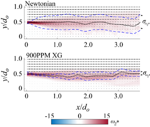
Figure 9. Time-averaged normalized-vorticity fields  $\overline {\omega ^{*}_{{z}}}$ with overlaid velocity vectors for the steady cases. In (a,c,e,g) cases at
  ${Re_{m}} = 4800$ are shown, and in (b,d, f,h) cases at
  ${Re_{m}} = 14\,400$ are shown. Time-averaged shear-layer properties for pure-water cases are shown in (a,b), 35 PPM in (c,d), 450 PPM in (e, f) and 900 PPM in (g,h). Every third vector is plotted for clarity. The dotted black line (
 $\cdots$) follows the maximum contour of
  $\overline {\omega ^{*}_{{z}}}$, representing the average shear-layer trajectory across
  $x/d_{{o}}$. Blue dashed lines (- - -, blue) represents plus-and-minus one standard deviation in the position of the average shear-layer trajectory.
The standard deviation of the shear-layer trajectory  $\sigma _{{\omega ^{*}_{{z}}}(y/d_{{o}})}$, which is determined by looking at the position of maximum normalized vorticity, reveals a correlation between the stabilization of the shear layer and shear-thinning strength;
  $\sigma _{{\omega ^{*}_{{z}}}(y/d_{{o}})}$ is plotted vs
  $x/d_{{o}}$ for
  ${Re_{m}} = 4800$ cases in figure 10(a), and
  ${Re_{m}} = 14\,400$ cases in figure 10(b). There is a marked decrease in the standard deviation with increasing shear-thinning strength, which demonstrates the increased tendency of instabilities to not deviate from
  $y/d_{{o}} = 0.5$. Reduced standard deviations with increasing shear-thinning strength is particularly clear in the
  ${Re_{m}} = 4800$ cases shown in figure 10(a) at a streamwise distance beyond
  $x/d_{{o}} > 2.5$. A similar trend is apparent in the standard deviations of the vorticity thickness as well, which demonstrates the predominance of concentrated instability cores for low shear-thinning cases vs a smeared shear layer in high shear-thinning cases. The reduction in standard deviations of both shear-layer trajectory and thickness further demonstrates the attenuation of instabilities and stabilization of the shear layer with increasing shear-thinning strength. At low shear-thinning strengths, instabilities present as concentrated vortex cores whose size and strength greatly affect the local thickness and trajectory of the shear layer. As the shear-thinning strength increases, the instabilities are attenuated, resulting in a shear layer with a far more stable thickness and trajectory. The authors stress that this correlation between shear-thinning strength and shear-layer stabilization is not very apparent when the Reynolds number is increased. This is apparent in figure 10(b) where, besides for the 900 PPM case, all standard deviations are not statistically different.

Figure 10. Standard deviation of the location of maximum vorticity  $\sigma _{{\omega ^{*}_{{z}}}(y/d_{{o}})}$ is plotted across
  $x/d_{{o}}$. Results for
  ${Re_m} = 4800$ and for
  ${Re_m} = 14\,400$ are included in (a) and (b), respectively. The standard deviation correlates with downstream distance and anti-correlates with shear-thinning strength. The region near
  $x/d_{{o}} = 1.5$ shows a slight increased noise spike due to the two-camera stitching region. Regions affected by non-physical artefacts in the
  ${Re_{m}} = 14\,400$ cases are omitted.
Far downstream of the expansion ( $x/d_{{o}} > 2.5$), the standard deviation of the shear-layer trajectory reduces with both increasing shear-thinning strength and
  ${Re_{m}}$. This is also apparent from the time-averaged vorticity fields in figure 9, where the standard deviation of the shear-layer trajectory is indicated by the distance between the upper and lower dashed lines. The reduction in standard deviation with shear-thinning strength is apparent within the low-Reynolds-number cases (left-column figures) and especially for the 900 PPM. However, this reduction with shear-thinning strength is far less apparent when the Reynolds number increases (right-column figures). The results complement observations from previous work, which show how shear-thinning fluids maintain turbulence within the dominant flow direction (Castro & Pinho Reference Castro and Pinho1995; Escudier & Smith Reference Escudier and Smith1999; Pereira & Pinho Reference Pereira and Pinho2000; Poole et al. Reference Poole, Escudier and Oliveira2005).
3.3. Steady flows: coalescence of vortical structures
It was observed from the instantaneous vorticity fields of the low- $Re$ steady shear-layer cases that KH instabilities were prone to coalesce while convecting downstream. This phenomena is further explored here using the normalized Reynolds shear-stress spectra
  $\varPhi _{u'v'/u_{{m}}^{2}}$, the intensities of which are plotted as colour maps in figure 11. Here,
  $u'$ and
  $v'$, respectively, represent the streamwise and vertical (stream-normal) fluctuating velocity components and are calculated by subtracting the time-averaged velocity from the total velocity. For the spectra presented here, we limit ourselves to the velocity content sampled along a horizontal line at
  $y/d_{{o}} = 0.5$ which is approximately the midpoint of the shear layer as shown in the steady time-averaged shear-layer vorticity results shown in figure 9. Spectral content is normalized using
  $d_{{o}}/2$, which is effectively a ‘step height’ (Poole & Escudier Reference Poole and Escudier2004). The spectral content is shown from
  $St = 0$ to 1.15 to focus on meaningful low-frequency content. The spectral intensity along
  $y/d_{{o}} = 0.5$ is plotted against streamwise distance (
 $x$-axis) and Strouhal number (
 $y$-axis), for
  ${Re_{m}} = 4800$ in figure 11(a–d) and for
  ${Re_{m}} = 14\,400$ in figure 11(e–h).

Figure 11. Normalized Reynolds stress spectra  $\varPhi _{u' v'/u_{{m}}^2}$ presented in relative decibels for steady shear-thinning fluid flows for cases at
  ${Re_{m}} = 4800$ in (a–d) and for cases at
  ${Re_{m}} = 14\,400$ in (e–h). Value of
  $\varPhi _{u' v'/u_{{m}}^2}$ for pure-water cases is shown in (a,e), 35 PPM in (b, f), 450 PPM in figures (c,g) and 900 PPM in (d,h). For the
  ${Re_{m}} = 4800$ cases, as shear-thinning strength increases, a general reduction in intensity occurs across the entire spectra, with the harmonics from the shedding persisting. This reduction in spectra occurs to a much lesser extent in the
  ${Re_{m}} = 14\,400$ cases, and the shedding harmonics are comparatively much more subdued.
Looking to the spectral results shown in figure 11, the regular shedding of the KH instability is indicated by the strong band of intensity at  $St = 0.18$. This regular shedding is particularly the case for the
  ${Re_{m}} = 4800$ cases in figure 11(a–d), but is somewhat subdued in the spectra for the
  ${Re_{m}} = 14\,400$ cases shown in figure 11(e–h). High-intensity spectral bands that are harmonics of the characteristic KH shedding frequency can be attributed to the ‘bursting’ of small-scale structures, where bursting represents the sudden splitting of structures into smaller structures. The harmonic bands are attributable to bursting at
  $x/d_{{o}} \le 1.0$ where this phenomenon was observed. Harmonics of
  $St = 0.18$ are also attributed to the flows’ largely monotonic behaviour and the self-interaction of dominant modes. Additionally, another small-scale structure signature exists at
  ${St} = 0.62$ for cases at
  ${Re_{m} = 14\,400}$.
As shear-thinning strength increases, fluctuations outside of the KH instabilities and their harmonics are attenuated. This is apparent from the spectral content of the  ${Re_{m}} = 4800$ cases shown in figure 11(a–d) and is indicative of the attenuation of small-scale structures observed in previous sections. A similar reduction in high-frequency spectral intensity is observed within the
  ${Re_{m}} = 14\,400$ cases shown in figure 11(e–h). Similar to what was observed within the high-
 ${Re_{m}}$ vorticity fields shown in figure 6, the reduction in spectral intensity is far more subdued for the high-
 ${Re_{m}}$ cases, which again suggests that turbulence is becoming the dominant mode of momentum transport (Back & Roschke Reference Back and Roschke1972).
For the  ${Re_{m}} = 4800$ cases, and especially within the strong shear-thinning fluid cases shown in figure 11(c,d), the low-frequency spectral content appears to grow more intense moving further downstream, which is possibly attributable to the coalescence of KH instabilities into larger rollers downstream of the sudden expansion and would suggest the existence of an inverse eddy cascade. The general increase in low-frequency spectral content with downstream distance appears to be enhanced with increasing shear-thinning strength. This correlates with how the regularity of coalescence also increases with shear-thinning strength, as observed within the
  ${Re_{m}} = 4800$ vorticity fields and supplementary movie 2. This increase in low-frequency spectral content is not apparent within the
  ${Re_{m}} = 14\,400$ cases, again suggesting that turbulence is becoming the dominant mode of momentum transport (Back & Roschke Reference Back and Roschke1972).
Further to the regular shedding of coherent structures, with regards to the low-Reynolds-number cases shown in figure 11(a–d), shear-layer flapping is prominent, which is indicated by low-frequency high-intensity spectra. In backwards-facing step flows, shear-layer flapping is known to affect the size of the recirculating region and consequently the fluid mixing, vorticity diffusion and shear-layer trajectory (Ma & Schröder Reference Ma and Schröder2017).
Although the spectra correlate with the trends observed within the instantaneous vorticity fields and reinforces the conclusion that shear-thinning strength promotes the attenuation of instabilities within the shear layer, the causation of this attenuation, the coalescence of structures and the self-organization of the spectra are unclear. One potential cause could be the streamwise reorientation and extension of xanthan gum polymer chains. The reorientation of the polymer chains would make them naturally stable against perturbations that tilt them off the streamwise axis, while the extension of polymer chains in the streamwise direction would absorb excess energy that would otherwise reorient into the stream-normal direction. This shear-thinning mechanism would effectively stratify the flow in the radial (stream-normal) direction about the axisymmetric expansion.
4. Conclusions
The current study investigates the formation of steady and unsteady ( $St = 0.15$) shear layers forming within fluids of increasing shear-thinning strength (
 $n = 1$, 0.81, 0.61 and 0.47) to characterize how shear-thinning strength affects the attenuation of coherent vortical structures. Test cases were performed at equivalent Reynolds numbers of
  ${Re_{m}} = 4800$ and 14 400. Based on previous studies, it was hypothesized that the large-scale flow topologies would be preserved while shear-layer instabilities would be attenuated.
The shear layers investigated herein were generated via an axisymmetric sudden expansion. Planar PIV measurements of the tested shear-layer cases were performed to extract measurements of their large-scale flow, as well as the embedded shear-layer instabilities. Measurements of large-scale flow, particularly the circulation in the unsteady cases and the vorticity thickness in steady cases, showed preservation of large-scale flow. Instantaneous vorticity fields for both unsteady and steady cases demonstrate how shear-layer instabilities attenuate from concentrated cores to smeared diffuse structures with increasing shear-thinning strength. This attenuation is especially true for the  ${Re_{{m}}} = 4800$ cases, whereas the
  ${Re_{{m}}} = 14\,400$ cases exhibit less dependence on shear-thinning strength due to increased turbulence. For steady shear layers, standard deviations of shear-layer trajectory and thickness were shown to reduce with increasing shear-thinning strength, confirming how instability attenuation and shear-layer stabilization correlate with shear-thinning strength.
The conclusion that shear-layer instabilities attenuate with increasing shear-thinning strength but to a lesser extent with increasing Reynolds number is reinforced by the fluctuation spectra along the midpoint of the shear layer: high-frequency content reduces with increasing shear-thinning strength for  ${Re_{{m}}} = 4800$ cases and less so for
  ${Re_{{m}}} = 14\,400$ cases. Finally, and especially for the low-
 ${Re_m}$ cases, the coalescing of instabilities into larger rollers was observed from instantaneous vorticity fields. The coalescence of instabilities into large rollers coincided with the increase of low-frequency spectral content with downstream distance. The coalescing of instabilities into rollers, coupled with the increase of low-frequency content with downstream distance, suggests an inverse eddy cascade within the flow.
The results show how shear-thinning fluids attenuate shear-layer instabilities and stabilize the shear layer, characteristics that complement observations made by previous studies (Castro & Pinho Reference Castro and Pinho1995; Escudier & Smith Reference Escudier and Smith1999; Pereira & Pinho Reference Pereira and Pinho2000; Poole et al. Reference Poole, Escudier and Oliveira2005). However, these characteristics are less present at high Reynolds numbers, at which point turbulence dominates momentum transport (Back & Roschke Reference Back and Roschke1972). Despite the results supporting our hypothesis, the cause behind the attenuation and coalescence of shear-layer instabilities is unclear. It is believed that the reorientation and extension of xanthan gum polymer chains in the streamwise plane may act to stabilize the flow against fluctuations, but this prediction is left for future work.
Supplementary movies
Supplementary movies are available at https://doi.org/10.1017/jfm.2024.1144.
Acknowledgements
M.B. acknowledges the support of Queen's University School of Graduate Studies and Postdoctoral Affairs (SGSPA) Duncan and Ullra Carmichael Fellowship.
Funding
We acknowledge the support of the Natural Sciences and Engineering Research Council of Canada (NSERC) (funding reference number ALLRP 569171-21).
Declaration of interests
The authors report no conflict of interest.


 Open access