2.1. Physical problem and the governing equations

The physical model to be studied is a polymer-solution flow in a round pipe. The flow field is analysed in the cylindrical coordinate system $(z,r,\theta )$, with $z$, $r$ and $\theta$ denoting the axial, radial and azimuthal directions, respectively. The pipe radius $R$ is selected as the reference length, and the velocity field $\boldsymbol u=(u_z,u_r,u_\theta )$, time $t$ and pressure $p$ are normalised by $U_{max}$, $R/U_{max}$ and $\rho U^{2}_{max}$, respectively, where $\rho$ is the density of the fluid, and $U_{max}$ is the maximum (centreline) velocity of the laminar pipe flow. The conformation tensor $\boldsymbol{\mathsf{c}}$ and stress $\boldsymbol \tau _p$ are normalised by $k_BT/H$ and $\mu _p U_{max}/R$, respectively, where $k_B$ is the Boltzmann constant, $T$ is temperature, $H$ is the spring constant in the elastic dumbbell model of the polymer, and $\mu _p$ is the additional fluid viscosity due to the polymer (Bird et al. Reference Bird, Curtiss, Armstrong and Hassager1987). The flow motions are characterised by, among others, two dimensionless parameters, a Reynolds number and a Weissenberg number, which are defined as

(2.1a,b)\begin{equation} Re=\frac{\rho U_{max}R}{\mu},\quad Wi=\frac{\lambda U_{max}}{R}, \end{equation}

where $\mu$ and $\lambda$ are the total viscosity and the relaxation time of the polymer molecules (to their equilibrium states), respectively. In particular, the total viscosity is the sum of the solvent viscosity $\mu _s$ and the polymer viscosity $\mu _p$, i.e. $\mu =\mu _s+\mu _p$, and a viscosity ratio $\beta$ is defined as

(2.2)\begin{equation} \beta=\frac{\mu_s}{\mu}\in[0,1]. \end{equation}

Note that if $\beta =1$, then the flow is Newtonian, while $\beta =0$ corresponds to the upper-convective-Maxwell (UCM) flow. The Oldroyd-B model is assumed (Bird et al. Reference Bird, Curtiss, Armstrong and Hassager1987), and the dimensionless Navier–Stokes equations and the constitutive equations are

(2.3a,b)$$\begin{gather} \boldsymbol{\nabla}\boldsymbol{\cdot} \boldsymbol u=0,\quad \frac{\partial \boldsymbol u}{\partial t}+\boldsymbol u\boldsymbol{\cdot}\boldsymbol{\nabla}\boldsymbol u={-}\boldsymbol{\nabla} p+\frac{\beta}{ Re}\nabla^{2}\boldsymbol u+\frac{1-\beta}{Re}\boldsymbol{\nabla}\boldsymbol{\cdot} \boldsymbol{\tau_p}, \end{gather}$$

(2.3c,d)$$\begin{gather}\boldsymbol{\tau_p}=\frac{{\boldsymbol{\mathsf{c}}}-\boldsymbol{\mathsf{I}} }{Wi},\quad \frac{\partial \boldsymbol{\mathsf{c}}}{\partial t}+\boldsymbol u\boldsymbol{\cdot}\boldsymbol{\nabla} \boldsymbol{\mathsf{c}}-\boldsymbol{\mathsf{c}}\boldsymbol{\cdot}(\boldsymbol{\nabla} \boldsymbol u)-(\boldsymbol{\nabla} \boldsymbol u)^{T}\boldsymbol{\cdot} \boldsymbol{\mathsf{c}} ={-}\boldsymbol{\tau_p}, \end{gather}$$

where $\boldsymbol{\mathsf{I}}$ denotes the unity matrix. Note that the Oldroyd-B model is an idealised model that assumes the polymer extensibility to be infinitely strong, which is sufficient to demonstrate the instability mechanism and convenient for analysis; therefore, we do not consider here the more realistic FENE-P model (where the effect of finite extensibility can be studied); see Zhang et al. (Reference Zhang, Lashgari, Zaki and Brandt2013), Lopez et al. (Reference Lopez, Choueiri and Hof2019), Page et al. (Reference Page, Dubief and Kerswell2020) and Zhang (Reference Zhang2021). As a systematic investigation, in the following we will visit the centre-mode instability in a complete set of the parameter space, which may include some unattainable $Wi$ in experiments.

The flow field $\boldsymbol \phi =(\boldsymbol u,p,{{\mathsf {c}}}_{11},{{\mathsf {c}}}_{12},{{\mathsf {c}}}_{22},{{\mathsf {c}}}_{13},{{\mathsf {c}}}_{23},{{\mathsf {c}}}_{33})$ is decomposed into a steady mean flow $\boldsymbol \varPhi =(\boldsymbol U,P,{{\mathsf {C}}}_{11},{{\mathsf {C}}}_{12},{{\mathsf {C}}}_{22},{{\mathsf {C}}}_{13},{{\mathsf {C}}}_{23},{{\mathsf {C}}}_{33})$ and a harmonic perturbation

(2.4)\begin{equation} \boldsymbol\phi=\boldsymbol\varPhi(r)+\hat\epsilon\, \boldsymbol{\hat\phi}(r)\,{{\rm e}}^{{{\rm i}}(k z+2{\rm \pi} m\theta-\omega t)}+{\rm c.c.},\end{equation}

where $\boldsymbol {\hat \phi }=(\boldsymbol {\hat u},\hat p,\hat {{\mathsf {c}}}_{11},\hat {{\mathsf {c}}}_{12},\hat {{\mathsf {c}}}_{22},\hat {{\mathsf {c}}}_{13},\hat {{\mathsf {c}}}_{23},\hat {{\mathsf {c}}}_{33})$, $\hat \epsilon \ll 1$ denotes the amplitude, $k$ is the axial wavenumber, $m$ is the number of waves in the azimuthal direction, $\omega$ is the frequency, and ${\rm c.c.}$ denotes the complex conjugate. In a temporal stability analysis, $k$ is taken to be real, and $\omega =\omega _r+{{\rm i}}\omega _i$ is complex, with the imaginary part representing the temporal growth rate. In this paper, we restrict our attention to the axisymmetric mode, for which $m=0$.

The base states $\boldsymbol \varPhi (r)$ for the velocity and conformation tensor field are expressed as

(2.5a,b)\begin{equation} \boldsymbol U=(U,0,0) \ \text{with} \ U=1-r^{2},\quad \boldsymbol C=\left( \begin{array}{ccc} 1+ 2Wi^{2}\,U'^{2} & Wi\,U' & 0 \\ Wi\,U' & 1 & 0 \\ 0 & 0 & 1 \end{array}\right),\end{equation}

where throughout this paper a prime denotes the derivative with respect to its argument.

In the above formulation, the conformation tensor is analysed in the sense of Reynolds decomposition, which has been adopted by many recent works on the centre-mode instability, such as Garg et al. (Reference Garg, Chaudhary, Khalid, Shankar and Subramanian2018), Page et al. (Reference Page, Dubief and Kerswell2020) and Chaudhary et al. (Reference Chaudhary, Garg, Subramanian and Shankar2021). We note that Hameduddin et al. (Reference Hameduddin, Meneveau, Zaki and Gayme2018) and Hameduddin, Gayme & Zaki (Reference Hameduddin, Gayme and Zaki2019) have recently proposed a new decomposition method based on a geometric understanding of the differential deformation of the polymers, being able to guarantee the positive-definiteness of the conformation tensor. For stability analyses of non-turbulent viscoelastic flows, the results of the two decomposition methods can be consistent with each other; see the comparisons in Zhang (Reference Zhang2021), Wan, Sun & Zhang (Reference Wan, Sun and Zhang2021) and Buza, Page & Kerswell (Reference Buza, Page and Kerswell2021).

2.2. Instability mode

After substituting (2.3c,d) into the governing equations (2.3) and retaining the $O(\hat \epsilon )$ terms, we arrive at a linear system of $\hat \phi$ for $m=0$:

(2.6a)$$\begin{gather} {{\rm i}}k \hat u_z+\hat u_r' +\hat u_r/r=0, \end{gather}$$

(2.6b)$$\begin{gather}{{\rm i}}k(U-c)\hat u_z+U'\hat u_r+{{\rm i}}k \hat p=\frac{\beta}{ Re}(\hat u_z''+\hat u_z'/r-k^{2}\hat u_z)+\frac{1-\beta}{{Re\,Wi}}({{\rm i}}k{\mathsf{\hat c}}_{11} +{\mathsf{\hat c}}_{12}'+{\mathsf{\hat c}}_{12}/r), \end{gather}$$

(2.6c)$$\begin{gather}{{\rm i}}k(U\!-\!c)\hat u_r+ \hat p'=\frac{\beta}{ Re}(\hat u_r''+\hat u_r'/r-k^{2} \hat u_r-\hat u_r/r^{2})\!+\!\frac{1-\beta}{{Re\,Wi}}({{\rm i}}k{\mathsf{\hat c}}_{12} +{\mathsf{\hat c}}_{22}'+{\mathsf{\hat c}}_{22}/r-{\mathsf{\hat c}}_{33}/r), \end{gather}$$

(2.6d)$$\begin{gather}({{\rm i}}k(U-c)+Wi^{{-}1}){\mathsf{\hat c}}_{11}+{\mathsf{C}}_{11}' \hat u_r-2({{\rm i}}k {\mathsf{C}}_{11} u_z+{\mathsf{C}}_{12}\hat u_z' +U'{\mathsf{\hat c}}_{12})=0, \end{gather}$$

(2.6e)$$\begin{gather}({{\rm i}}k(U-c)+Wi^{{-}1}){\mathsf{\hat c}}_{12}+{\mathsf{C}}_{12}'\hat u_r-({{\rm i}}k{\mathsf{C}}_{12} u_z+{\mathsf{C}}_{22}\hat u_z'+U'{\mathsf{\hat c}}_{22}+{{\rm i}}k {\mathsf{C}}_{11}\hat u_r+{\mathsf{C}}_{12}\hat u_r')=0, \end{gather}$$

(2.6f)$$\begin{gather}({{\rm i}}k(U-c)+Wi^{{-}1}){\mathsf{\hat c}}_{22}-2({{\rm i}}k {\mathsf{C}}_{12} u_r+{\mathsf{C}}_{22}\hat u_r')=0, \end{gather}$$

(2.6g)$$\begin{gather}({{\rm i}}k(U-c)+Wi^{{-}1}){\mathsf{\hat c}}_{33}-2{\mathsf{C}}_{33} \hat u_r/r=0, \end{gather}$$

where $c\equiv \omega /k=c_r+{{\rm i}}c_i$, with $c_r$ denoting the phase speed. This system is an extension of the Orr–Sommerfeld equations, and so is referred to as the EOS system in this paper. No-slip, non-penetration conditions are imposed at the wall:

(2.7a,b)\begin{equation} \hat u_z(1)=\hat u_r(1)=0.\end{equation}

At the centreline, the radial velocity must vanish due to the symmetric nature, and we obtain from the continuity equation that the axial velocity must have zero gradient. Therefore, the boundary conditions at $r=0$ are

(2.8a,b)\begin{equation} \hat u'_z(0)=\hat u_r(0)=0.\end{equation}

2.3. Brief overview of numerical solutions of the EOS system

Using numerical code as implemented in Zhang (Reference Zhang2021), we can obtain solutions to the EOS system (2.6) with boundary conditions (2.7) and (2.8). The calculated eigenspectra, including the continuous and discrete modes, are compared with those of Chaudhary et al. (Reference Chaudhary, Garg, Subramanian and Shankar2021) in Appendix A, and favourable agreement is achieved.

The linear system (2.6) is dependent on four control parameters, $Re$, $Wi$, $k$ and $\beta$, and the unstable centre mode appears in a certain range of them. For a fixed $\beta$, the critical parameters $Re_c$, $Wi_c$ and $k_c$, depicting the onset of axisymmetric neutral instability, form a three-dimensional curve in the $Re$–$Wi$–$k$ space. For demonstration, we choose $\beta =0.9$ and plot the projections of this curve onto the $Re$–$Wi$ and $k$–$Wi$ planes in figures 1(a) and 1(b), respectively. 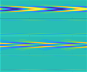The unstable zone appears when $Wi$ is greater than approximately 56, and two critical neutral curve branches appear for each supercritical $Wi$. As $Wi$ becomes large, $k_c$ for the lower-branch neutral curve is decreasing, whereas $k_c$ for the upper-branch neutral curve is increasing. A similar plot can be found in Buza et al. (Reference Buza, Page and Kerswell2021) for an FENE-P channel flow.

Figure 1. Projections of the critical neutral curve for $\beta =0.9$ and $m=0$ in the $Wi$–$Re$ (a) and $Wi$–$k$ (b) planes.

By visiting a large set of control parameters, Chaudhary et al. (Reference Chaudhary, Garg, Subramanian and Shankar2021) presented interesting observations on the centre instability. (1) For fixed $\beta$ and $E\equiv Re/Wi$, the neutral curves in the $Re$–$k$ and $c_r$–$k$ planes exhibit scattered behaviour without any regular pattern; however, when they are plotted in $Re\,E^{3/2}$–$kE^{1/2}$ and $(1-c_r)/E$–$kE^{1/2}$ planes, the curves with different $E$ collapse perfectly. (2) In the limit as $\beta \rightarrow 1$, the neutral curves can be scaled in the $Re[(1-\beta )E]^{3/2}$–$k[(1-\beta )E]^{1/2}$ plane. (3) By use of regular perturbation techniques, two regimes, with central-layer thicknesses $O(Re^{-1/3}R)$ and $O(Re^{-1/4}R)$, respectively, were found, which are able to predict the numerical eigenfunctions for a few selections of parameters. However, these observations lack in-depth explanations, and the physical origin of the centre-mode instability remains unclear. As the lower and upper branches of the neutral curve shown in figure 1 correspond to low and high limits of the critical wavenumbers, respectively, it is natural to link these two limits to the potentially distinguished long- and short-wavelength regimes in the asymptotic framework, respectively. Analysis of these regimes could explain the numerical observations of Chaudhary et al. (Reference Chaudhary, Garg, Subramanian and Shankar2021), and shed light on the key mechanism of the centre-mode instability, which is to be presented in §§ 3 and 4.

2.4. Summary of the overall structures of the asymptotic regimes

Before illustrating the mathematical details of the asymptotic regimes, we summarise the salient observations from§§ 3 and 4. A schematic of the multi-layered structure for both the long- and short-wavelength regimes is shown in figure 2. Usually, three asymptotic layers, including a wall layer, a main layer and a central layer, appear in the radial direction, but an additional critical layer may appear when the concentration is low ($\beta \rightarrow 1$) and the mode is near neutral. Table 1 summarises the asymptotic scalings and the thickness of each asymptotic layer, where a few quantities are to be defined in the following two sections. Readers can use this table as a guide to understand §§ 3 and 4.

Figure 2. A sketch of the multi-layered structure for long-wavelength centre modes in a viscoelastic pipe flow. The critical layer appears only for near-neutral low-concentration centre modes.

Table 1. Summary of the asymptotic regimes, including the scaling relations of the control parameters, similarity parameters and thickness of each asymptotic layer in viscoelastic pipe flows.

Note that in the regular-concentration regime, as will be discussed in §§ 3.1 and 4.1, no singularity appears in the central-layer solution, so the critical layer is not needed. However, we do need a critical layer in the low-concentration regime, as will be shown in §§ 3.2 and 4.2.

3.1. Asymptotic analysis for a regular-level concentration

The viscosity ratio in this subsection is assumed to be $O(1)$, but not close to unity:

(3.4a,b)\begin{equation} \beta=O(1),\quad 1-\beta=O(1).\end{equation}

Preliminary asymptotic analysis indicates that three asymptotic layers appear in the radial direction, as listed in table 1. In the wall layer, the viscosity appears at leading order, and from balance of the convective and viscous terms, we obtain the thickness of the wall layer,

(3.5)\begin{equation} 1-r=O(k^{{-}1/2} Re^{{-}1/2}). \end{equation}

The central layer may be driven by either viscosity or elasticity. From balance of the convective term of the conformation tensor ${{\rm i}}k (U-c){\hat {{\mathsf {c}}}}_{ij}$ with the conformation stress $Wi^{-1}{\hat {{\mathsf {c}}}}_{ij}$, noticing that $U=1-r^{2}$ and the phase speed $c$ is rather close to 1, we can estimate the thickness of the elastic central layer as

(3.6)\begin{equation} r=O(k^{{-}1/2}Wi^{{-}1/2}).\end{equation}

On the other hand, from balance of the convective terms in the axial momentum equation with the viscous terms, we obtain the thickness of the viscous central layer as

(3.7)\begin{equation} r=O(k^{{-}1/4} Re^{{-}1/4}).\end{equation}

Note that the thicknesses of the two central layers are usually of different magnitudes, depending on the values of the control parameters, $Re$, $Wi$ and $k$. In this paper, we will show that an unstable centre mode could appear when the thicknesses of the two layers are comparable, which leads to a scaling law

(3.8)\begin{equation} Wi\sim k^{{-}1/2} Re^{1/2},\end{equation}

rendering a viscoelasticity instability nature.

For convenience, we introduce

(3.9a–{–} c)\begin{equation} R_1= Re/\beta, \quad W_1=k^{1/2}R_1^{{-}1/2}Wi,\quad W_2=\beta W_1/(1-\beta). \end{equation}

From assumptions (3.1) and (3.4a,b), we know that $R_1=O( Re)$ and $(W_1,W_2)=O(1)$. In the central layer, from (3.6) or (3.7), balance of the axial momentum equation determines that the correction of the phase speed is $O(r^{2})=O(k^{-1/2}R_1^{-1/2})$. Therefore, we expand the complex phase speed in terms of an asymptotic series

(3.10)\begin{equation} c=1+k^{{-}1/2}R_1^{{-}1/2}c_1+\cdots,\end{equation}

in which the first term on the right-hand side, 1, comes from the centreline velocity of the base flow. The next task is to solve for $c_1$ to gain a more quantitative understanding of the instability. In the following three subsections, we will show the leading-order governing equations and their solutions for the three asymptotic layers.

3.1.1. Main-layer solutions

In the main layer (layer II of figure 2), we obtain from the continuity equation (2.6a) that $\hat u_r\sim k\hat u_z$. Balance of the conformation equations determines ${\hat {{\mathsf {c}}}}_{11}\sim k^{-1}R_1\hat u_z$, ${\hat {{\mathsf {c}}}}_{12}\sim R_1\hat u_z$ and ${\hat {{\mathsf {c}}}}_{22}\sim k^{1/2}R_1^{1/2}\hat u_z$. Therefore, the perturbation field is expanded as

(3.11a)$$\begin{gather} (\hat u_z,\hat u_r,\hat p)=(\hat u_0,k\hat v_0,\hat p_0)+k^{{-}1/2}R_1^{{-}1/2}(\hat u_1,k\hat v_1,\hat p_1)+\cdots, \end{gather}$$

(3.11b)$$\begin{gather}({\mathsf{\hat c}}_{11},{\mathsf{\hat c}}_{12},{\mathsf{\hat c}}_{22})=(k^{{-}1}R_1{\mathsf{\hat c}}_{11,0},R_1{\mathsf{\hat c}}_{12,0},k^{1/2}R_1^{1/2}{\mathsf{\hat c}}_{22,0})+\cdots. \end{gather}$$

In the main layer, the viscosity and polymer stress tensor play minor roles to the momentum convection, so the leading-order governing equations for the hydrodynamic perturbations are

(3.12a–c)\begin{equation} {{\rm i}} \hat u_0+\hat v_0'+\hat v_0/r=0, \quad -{{\rm i}}r^{2}\hat u_0-2r\hat v_0+{{\rm i}} \hat p_0=0,\quad \hat p_0'=0,\end{equation}

which implies the inviscid nature to leading-order accuracy. The solutions of (3.12) are $\hat u_0=2{{\rm i}}A_1$, $\hat v_0={{{\rm i}}\hat p_0}/({2r})+A_1r$, with $A_1$ being an arbitrary constant. These solutions do not satisfy the no-slip condition at the wall, $r=1$, which indicates that a viscous wall layer (layer I) must be taken into account. The analysis of this layer is the same as that of the Stokes layer in Goldstein (Reference Goldstein1985), Liu, Dong & Wu (Reference Liu, Dong and Wu2020) and Dong, Liu & Wu (Reference Dong, Liu and Wu2020). It was shown that the radial velocity $\hat v_r$ is much smaller than the axial velocity $\hat v_z$ due to its thin-layer property, which determines the boundary condition of the main layer at the wall, $\hat v_0(1)=0$. A direct consequence is $A_1=-{{{\rm i}}\hat p_0}/{2}$. Therefore, the solutions of the leading-order velocities are

(3.13a,b)\begin{equation} \hat u_0=\hat p_0,\quad \hat v_0=\frac{{{\rm i}}\hat p_0}{2}\left(\frac 1r-r\right).\end{equation}

The governing equations for the leading-order conformation tensor are

(3.14a)\begin{gather} -{{\rm i}}r^{2}{\mathsf{\hat c}}_{11,0}+16W_1^{2}r\hat v_0+4r{\mathsf{\hat c}}_{12,0}-16W_1^{2}{{\rm i}}r^{2}\hat u_0=0, \end{gather}

(3.14b,c)\begin{gather} -{{\rm i}}r^{2}{\mathsf{\hat c}}_{12,0}-8{{\rm i}}r^{2} W_1^{2}\hat v_0=0,\quad -{{\rm i}}r^{2}{\mathsf{\hat c}}_{22,0}+4{{\rm i}}r W_1\hat v_0 =0, \end{gather}

whose solutions are

(3.15a–c)\begin{equation} {\mathsf{\hat c}}_{11,0}={-}16{{\rm i}}W_1^{2} \hat v'_0,\quad {\mathsf{\hat c}}_{12,0}={-}8W_1^{2}\hat v_0,\quad {\mathsf{\hat c}}_{22,0}=\frac{4W_1}{r}\hat v_0.\end{equation}

The second-order hydrodynamic perturbations are governed by

(3.16a)\begin{gather} {{\rm i}} \hat u_1+\hat v_1'+\hat v_1/r=0, \end{gather}

(3.16b,c)\begin{gather} -{{\rm i}}r^{2}\hat u_1-2r\hat v_1+{{\rm i}} \hat p_1={{\rm i}}c_1\hat u_0+ W_2^{{-}1}({{\rm i}} {\mathsf{\hat c}}_{11,0}+{\mathsf{\hat c}}_{12,0}'+{\mathsf{\hat c}}_{12,0}/r), \quad \hat p_1'=0, \end{gather}

from which we obtain

(3.17)\begin{equation} \hat v_1=\frac{{{\rm i}} \hat p_1}{2r}+{{\rm i}}\hat p_0\left(\frac{2 W_1^{2}W_2^{{-}1}}{r^{3}}-\frac{ c_1}{2r}\right)-\left(\frac{{{\rm i}} \hat p_1}{2}+{{\rm i}}\hat p_0(2W_1^{2}W_2^{{-}1}-c_1/2)+A_2\right)r, \end{equation}

where $A_2$ is a constant. In principle, $A_2$ can be determined by matching with the wall-layer solution, but it is not needed in the following analysis.

Combining (3.13a,b) and (3.16a), we obtain the asymptotic behaviours of the velocity field in the limit as $r\rightarrow 0$:

(3.18a)$$\begin{gather} \hat u_r\rightarrow \frac{{{\rm i}} \hat p_0}{2}k\left(\frac{1}{r}+\cdots+4 k^{{-}1/2} R_1^{{-}1/2}W_1^{2}W_2^{{-}1}\frac{1}{r^{3}}+\cdots\right), \end{gather}$$

(3.18b)$$\begin{gather}\hat u_z\rightarrow \hat p_0\left(1+\cdots +4 k^{{-}1/2} R_1^{{-}1/2}W_1^{2}W_2^{{-}1}\frac 1{r^{4}}+\cdots\right). \end{gather}$$

Obviously, these solutions cease to be valid when the high-order terms come to the leading order, which appears in the vicinity of the centreline. From (3.18b) we find that a sublayer appears when $r=O(k^{-1/8}R_1^{-1/8})$. However, a further analysis indicates that this layer is not a distinguished one because the leading-order impact does not change. From (3.18a) we find that a sublayer appears when $r=O(k^{-1/4}R_1^{-1/4})$, which is the same as the central layer (3.7).

3.1.2. Viscous wall layer

Since the inviscid solution in the main layer does not satisfy the no-slip condition at the wall, a wall (Stokes) layer for which $1-r=O(k^{-1/2}R_1^{-1/2})$ needs to be considered. For convenience, we introduce a local coordinate

(3.19)\begin{equation} \hat y=(1-r)k^{1/2}R_1^{1/2}=O(1). \end{equation}

The flow field is expanded as

(3.20)\begin{equation} (\hat u_z,\hat u_r,\hat p)=\hat p_0(\hat u_w,k^{1/2}R_1^{{-}1/2}\hat v_w,\hat p_w)+\cdots,\end{equation}

and the influence of the polymer stress is of high-order impact in this layer.

The leading-order governing equations in the wall layer are

(3.21a–c)\begin{equation} {{\rm i}} \hat u_w+\hat v_w'=0,\quad-{{\rm i}} \hat u_w-{{\rm i}}\hat p_w-\hat u''_w=0,\quad \hat p_w'=0. \end{equation}

Eliminating $\hat v_w$ and $\hat p_w$, we obtain

(3.22)\begin{equation} \hat u_w=\hat p_w\left(1-\exp({{{\rm e}}^{{3{\rm \pi}{{\rm i}}}/4}\hat y})\right). \end{equation}

Matching with the main-layer solution, we obtain that $\hat p_w=1.$

3.1.3. Central layer

Because the expansion (3.11a) breaks down in the $O(k^{-1/4}R_1^{-1/4})$ vicinity of the centreline, we need to carry out an analysis in this layer. For convenience, we introduce the local coordinate

(3.23)\begin{equation} \tilde y=k^{1/4}R_1^{1/4}r=O(1).\end{equation}

The perturbation field is now expanded as

(3.24a)$$\begin{gather} (\hat v_z,\hat v_r,\hat p)= \hat p_0 (k^{1/2}R_1^{1/2}\tilde u,k^{5/4}R_1^{1/4} \tilde v,1)+\cdots, \end{gather}$$

(3.24b)$$\begin{gather}({\mathsf{\hat c}}_{11},{\mathsf{\hat c}}_{12},{\mathsf{\hat c}}_{22})= \hat p_0 (k^{{-}1/2}R_1^{3/2}{\mathsf{\tilde c}}_{11},k^{1/4}R_1^{5/4}{\mathsf{\tilde c}}_{12},kR_1{\mathsf{\tilde c}}_{22})+\cdots. \end{gather}$$

Substitution of (3.24) into (2.6) leads to

(3.25a)$$\begin{gather} {{\rm i}} \tilde u+\tilde v'+\tilde v/\tilde y=0, \end{gather}$$

(3.25b)$$\begin{gather}-{{\rm i}} (\tilde y^{2}+c_1)\tilde u-2\tilde y\tilde v+{{\rm i}}=\tilde u''+\tilde u'/\tilde y+W_2^{{-}1}({{\rm i}}{\mathsf{\tilde c}}_{11}+{\mathsf{\tilde c}}_{12}'+{\mathsf{\tilde c}}_{12}/\tilde y), \end{gather}$$

(3.25c)$$\begin{gather}\tilde L{\mathsf{\tilde c}}_{11}=16{{\rm i}}W_1^{2} \tilde y^{2}\tilde u-4W_1 \tilde y \tilde u'-4\tilde y{\mathsf{\tilde c}}_{12}-16W_1^{2}\tilde y\tilde v, \end{gather}$$

(3.25d)$$\begin{gather}\tilde L{\mathsf{\tilde c}}_{12}=\tilde u'-2{{\rm i}}W_1 \tilde y\tilde u-2 \tilde y{\mathsf{\tilde c}}_{22}-2W_1 \tilde y\tilde v'+2W_1\tilde v+8{{\rm i}} \tilde y^{2}W_1^{2}\tilde v, \end{gather}$$

(3.25e)$$\begin{gather}\tilde L{\mathsf{\tilde c}}_{22}=2\tilde v'-4{{\rm i}}W_1 \tilde y\tilde v, \end{gather}$$

where $\tilde L\equiv -{{\rm i}} ( \tilde y^{2}+c_1)+W_1^{-1}$. In (3.25b), both the viscosity and the polymer stress tensor appear at leading order, therefore this equation is not singular at any radial position. In (3.25c–e), it is seen that there is no viscous-like term (second-order derivative with respect to $\tilde y$) on the right-hand sides, and a singularity is possible when $\tilde L=0$, which, however, occurs only for $c_{1,i}=-W_1^{-1}$. Since $W_1>0$, such a condition implies that the eigenmode is stable with an exponentially decaying manner, which is of little interest in our study. Therefore, in the following analysis of the long-wavelength regular-concentration unstable (or marginally unstable) mode, we do not need a critical layer.

Note that the equation system does not admit closed-form analytical solutions, so we seek help from numerics. In the numerical process, the system (3.25) can be recast to a group of first-order differential equations

(3.26)\begin{equation} \frac{{{\rm d}} {\tilde{\boldsymbol \phi}}}{{{\rm d}} \tilde y}=\tilde{\boldsymbol L} \tilde{\boldsymbol \phi}, \end{equation}

where $\tilde {\boldsymbol \phi }=(\tilde u,\tilde u',\tilde u'',\tilde v)^{T}$ and the non-zero elements of $\tilde {\boldsymbol L}$ are

(3.27)$$\begin{gather} {\mathsf{\tilde L}}_{12}=1,\quad {\mathsf{\tilde L}}_{23}=1,\quad {\mathsf{\tilde L}}_{31}=\frac{16W_1^{2}\tilde y(\tilde y^{4}- c_1^{2})}{\tilde L^{2}(1+ W_2\tilde L)},\quad {\mathsf{\tilde L}}_{41}={-}{{\rm i}},\quad {\mathsf{\tilde L}}_{44}={-}1/\tilde y, \end{gather}$$

(3.28)$$\begin{gather}{\mathsf{\tilde L}}_{32}= \frac{8\tilde y^{4}-8\tilde y^{2}({{\rm i}} +2 W_1\tilde y^{2})\tilde L+(1+8{{\rm i}}W_1\tilde y^{2}+8 W_1^{2}\tilde y^{4})\tilde L^{2}}{\tilde y^{2}\tilde L^{2} (1+ W_2\tilde L)}+\frac{{ W_2}(1-{{\rm i}} \tilde y^{2}(\tilde y^{2}+ c_1))\tilde L^{3}}{\tilde y^{2}\tilde L^{2} (1+ W_2\tilde L)}, \end{gather}$$

(3.29)$$\begin{gather}{\mathsf{\tilde L}}_{33}={-}\frac{4{{\rm i}} \tilde y^{2}+\tilde L-4{{\rm i}} \tilde W_1\tilde y^{2}\tilde L+ W_2\tilde L^{2}}{\tilde y\tilde L(1+ W_2\tilde L)},\quad {\mathsf{\tilde L}}_{34}={-}\frac{32 {{\rm i}}W_1^{2}\tilde y^{2}(\tilde y^{2}- c_1)}{\tilde L^{2}(1+ W_2\tilde L)}. \end{gather}$$

Matching with the main-layer solutions (3.18b), we obtain the matching conditions

(3.30a,b)\begin{equation} \tilde u\rightarrow \frac{4W_1^{2}W_2^{{-}1}}{\tilde y^{4}}+o(\tilde y^{{-}4}),\quad \tilde v\rightarrow \frac{{{\rm i}}}{2\tilde y}+O(\tilde y^{{-}3})\quad\mbox{as }\tilde y\rightarrow \infty. \end{equation}

In the numerical process, this condition can be recast as

(3.31)\begin{equation} (\tilde u',\tilde u'')\rightarrow 0\quad \mbox{at }\tilde y=\tilde y_n, \end{equation}

with $\tilde y_n\gg 1$ being the upper boundary of the computational domain. The boundary conditions at the centreline are

(3.32)\begin{equation} \tilde u'(0)=\tilde v(0)=0.\end{equation}

The system (3.26) with (3.31) and (3.32) is to be solved numerically by the same approach as in Dong & Wu (Reference Dong and Wu2013) and Wu & Dong (Reference Wu and Dong2016). It is obvious from this system that for a given $\beta$, the eigenvalue, $c_1$, and the eigenfunctions depend on only one parameter, $W_1=k^{1/2}R_1^{-1/2}Wi$, which reduces the complexity of the original eigenvalue system remarkably. Practically, with the assumptions (3.1) and (3.9a–c), we know that $Wi$ has to be much greater than unity. For a given $\beta$ that is not close to unity, the unstable centre modes would appear in a certain range of $W_1$, and the unstable region of $Wi$ increases with $Re^{1/2}$ and decreases with $k^{-1/2}$.

3.2. Asymptotic analysis for a low-level concentration

As $\beta$ approaches unity, $W_2$ in (3.9a–c) becomes much greater than 1, and the asymptotic analysis in § 3.1 needs to be modified. For convenience, we introduce

(3.33)\begin{equation} \sigma=\frac{1-\beta}{\beta}\ll 1. \end{equation}

Balancing the leading-order terms in the central layer, we can work out that $W_1\sim \sigma ^{-1}$. Here we have assumed $k^{1/2}R_1^{-1/2}\ll \sigma \ll 1$. For convenience, we introduce an $O(1)$ parameter $\bar W$ such that

(3.34a,b)\begin{equation} W_1=\sigma^{{-}1}\bar W,\quad W_2=\sigma^{{-}2}\bar W.\end{equation}

The complex phase speed is now expanded as

(3.35)\begin{equation} c=1+k^{{-}1/2}R_1^{{-}1/2}(\bar c_1+\sigma\bar c_2)+\cdots.\end{equation}

In the following, we will study the three asymptotic layers in the low-concentration configuration. The overall process is the same as that in § 3.1, but in this regime, a critical layer, as sketched in figure 2, appears in the central layer when the mode is neutral.

3.2.1. Main layer

Following the same procedure as in § 3.1.1, we obtain the main-layer radial velocity perturbation in the limit as $r\rightarrow 0$:

(3.36)\begin{equation} \hat u_r\rightarrow \frac{{{\rm i}} \hat P_0}{2}k\left(\frac{1}{r}+\cdots+4 k^{{-}1/2} R_1^{{-}1/2}\bar W\frac{1}{r^{3}}+\cdots\right),\end{equation}

where $\hat P_0$ denotes the pressure perturbation in the main layer. Note that the solutions in the wall layer (3.20) stay unchanged.

3.2.2. Central layer

The thickness of the central layer in this regime is the same as that in § 3.1.3, so $\tilde y$ in (3.23) is still the local coordinate. The perturbation field is expanded as

(3.37a)$$\begin{gather} (\hat v_z,\hat v_r,\hat p)= \hat p_0 [k^{1/2}R_1^{1/2}(\tilde U_0+ \sigma\tilde U_1),k^{5/4}R_1^{1/4} (\tilde V_0+\sigma\tilde V_1),(1+ \sigma\tilde P_1)]+\cdots, \end{gather}$$

(3.37b)$$\begin{gather}({\mathsf{\hat c}}_{11},{\mathsf{\hat c}}_{12},{\mathsf{\hat c}}_{22})= \hat p_0 (k^{{-}1/2}R_1^{3/2}\sigma^{{-}2}{\mathsf{\tilde C}}_{11},k^{1/4}R_1^{5/4}\sigma^{{-}2}{\mathsf{\tilde C}}_{12},kR_1\sigma^{{-}1}{\mathsf{\tilde C}}_{22})+\cdots. \end{gather}$$

Since $W_1$ and $W_2$ are much greater than 1, the leading-order governing equations are changed to

(3.38a)$$\begin{gather} {{\rm i}} \tilde U_0+\tilde V'_0+\tilde V_0/\tilde y=0, \end{gather}$$

(3.38b)$$\begin{gather}\tilde L_1\tilde U_0-2\tilde y\tilde V_0+{{\rm i}}=\tilde U''_0+\tilde U'_0/\tilde y+\bar W^{{-}1}({{\rm i}} {\mathsf{\tilde C}}_{11,0}+{\mathsf{\tilde C}}_{12,0}'+{\mathsf{\tilde C}}_{12,0}/\tilde y), \end{gather}$$

(3.38c)$$\begin{gather}\tilde L_1{\mathsf{\tilde C}}_{11,0}=16{{\rm i}} \bar W^{2} \tilde y^{2}\tilde U_0-4\tilde y{\mathsf{\tilde C}}_{12,0}-16\bar W^{2}\tilde y\tilde V_0, \end{gather}$$

(3.38d,e)$$\begin{gather}\tilde L_1{\mathsf{\tilde C}}_{12,0}=8{{\rm i}} \tilde y^{2}\bar W^{2}\tilde V_0,\quad \tilde L_1{\mathsf{\tilde C}}_{22,0}={-}4{{\rm i}} \bar W \tilde y\tilde V_0, \end{gather}$$

where $\tilde L_1=-{{\rm i}} ( \tilde y^{2}+\bar c_1)$. Comparing with (3.25), it is found that a few terms in the conformation tensor equations move to the high order. However, they may become the leading-order impact if $\tilde L_1\approx 0$ somewhere inside the central layer. This situation occurs when the mode to leading order is neutral, i.e. $\bar c_1$ is real and negative. Therefore, for the neutral case, a critical layer around $\tilde y_c=\sqrt {-\bar c_1}$, with thickness $\tilde y-\tilde y_c=O(\sigma )$ (or $r-r_c=O(\sigma k^{-1/4}R_1^{-1/4})$ with $r_c=k^{-1/4}R_1^{-1/4}\tilde y_c$), must be taken into account; see the red region of figure 2. A detailed analysis of the critical layer is provided in Appendix C.

Being similar to (3.26), the system (3.38) is recast to

(3.39)\begin{equation} \frac{{{\rm d}} {\tilde{\boldsymbol \phi}_0}}{{{\rm d}} \tilde y}={\boldsymbol L} \tilde{\boldsymbol \phi}_0,\end{equation}

where $\tilde {\boldsymbol \phi }_0=(\tilde U_0,\tilde U_0',\tilde U_0'',\tilde V_0)^{T}$ and

(3.40)\begin{equation} {\boldsymbol L}=\left( \begin{array}{cccc} 0 & 1 & 0 & 0 \\ 0 & 0 & 1 & 0 \\ \displaystyle \dfrac{16\bar W\tilde y(2{{\rm i}}\tilde y^{2}+\tilde L_1)}{\tilde L_1^{2}} & \displaystyle\dfrac 1{\tilde y^{2}}+\dfrac{8\bar W\tilde y^{2}}{\tilde L_1}+\tilde L_1 & \displaystyle -\dfrac 1{\tilde y} & \displaystyle\dfrac{-32\bar W\tilde y^{2}(2{{\rm i}}\tilde y^{2}+\tilde L_1)}{\tilde L^{3}_1} \\ -{{\rm i}} & 0 & 0 & -1/\tilde y \\ \end{array} \right). \end{equation}

The linear system (3.39) is subject to the matching and boundary conditions (3.31) and (3.32), with $(\hat u,\hat v)$ being replaced by $(\hat U_0,\hat V_0)$.

In order to obtain $\bar c_2$, we need to consider the second-order perturbations, which are governed by

(3.41)\begin{equation} \left(\frac{{{\rm d}}}{{{\rm d}} \tilde y}-{\boldsymbol L}\right)\tilde{\boldsymbol \phi}_1=\boldsymbol b, \end{equation}

where $\tilde {\boldsymbol \phi }_1=(\tilde U_1,\tilde U_1',\tilde U_1'',\tilde V_1)^{T}$ and $\boldsymbol b=(0,0,b_1\bar c_2+b_2,0)$, with

(3.42)$$\begin{gather} b_1=\frac{8\bar W\tilde y}{\tilde L_1^{4}}[{-8\tilde y\tilde L_1(\tilde y\tilde U_0+{{\rm i}}\tilde V_0)+24\tilde y^{3}\tilde V_0+{{\rm i}}\tilde L_1^{2}(2\tilde U_0+\tilde y\tilde U_0')}]-{{\rm i}}\tilde U_0', \end{gather}$$

(3.43)$$\begin{gather}b_2=\frac{4{{\rm i}}}{\tilde L_1^{4}}[{-}24\tilde y^{2}\tilde L_1(\tilde y\tilde U_0+{{\rm i}}\tilde V_0)+48\tilde y^{4}\tilde V_0+6{{\rm i}}\tilde y\tilde L_1^{2}(2\tilde U_0+\tilde y\tilde U_0')+\tilde L_1^{3}(2\tilde U_0'+\tilde y\tilde U_0'')]. \end{gather}$$

The adjoint vector ${\boldsymbol \psi }^{{\dagger} }=({\boldsymbol \psi }^{{\dagger} }_{1},{\boldsymbol \psi }^{{\dagger} }_{2}, {\boldsymbol \psi }^{{\dagger} }_{3},{\boldsymbol \psi }^{{\dagger} }_{4})^{T}$ of the differential equation (3.39) satisfies

(3.44)\begin{equation} \left(\frac{{{\rm d}}}{{{\rm d}} \tilde y}+{\boldsymbol L}^{T}\right){\boldsymbol\psi}^{{\dagger}}=0, \end{equation}

with the matching and boundary conditions

(3.45a,b)\begin{equation} {\boldsymbol\psi}^{{\dagger}}_{2,3}(\tilde y)\rightarrow 0\ \mbox{as}\ \tilde y\rightarrow \infty,\quad {\boldsymbol\psi}^{{\dagger}}_{1}(0)={\boldsymbol\psi}^{{\dagger}}_{3}(0)=0. \end{equation}

After multiplying both sides of (3.41) by $({\boldsymbol \psi }^{{\dagger} })^{T}$ and integrating from $\tilde y=0$ to $\infty$, we obtain the second-order correction of the phase speed:

(3.46)\begin{equation} \bar c_2={-}\frac{\displaystyle \int_0^{\tilde y}\psi^{{\dagger}}_{3}b_2\, {{\rm d}} \tilde y}{\displaystyle \int_0^{\tilde y}\psi^{{\dagger}}_{3}b_1\, {{\rm d}} \tilde y}.\end{equation}

4.1. Asymptotic analysis for a regular-level concentration

In this regime, the leading-order balance of the central layer is the same as that in the long-wavelength regime, so the relation (3.8) is also valid. However, because in this regime $k\gg 1$, we obtain from balance of the leading-order terms of the linearised system (2.6) in each layer that the instability appears when

(4.1a–c)\begin{equation} Re=O(k^{3}),\quad Wi=O(k),\quad \beta=O(1), \end{equation}

therefore a group of $O(1)$ parameters is introduced:

(4.2a–c)\begin{equation} R_3=k^{{-}3} Re/\beta,\quad W_3=k^{{-}1}R_3^{{-}1/2}Wi,\quad W_4=\beta W_3/(1-\beta). \end{equation}

By scaling analysis as in the previous section, we expand the complex phase speed as

(4.3)\begin{equation} c=1+k^{{-}2}R_3^{{-}1/2}\hat c_1+\cdots. \end{equation}

The asymptotic structure of the instability is the same as in figure 2, which is to be analysed in the following subsections.

4.1.1. Main-layer solution

Being similar to the long-wavelength mode, the governing equations in the main layer are inviscid to leading-order accuracy. The short-wavelength perturbation usually oscillates rapidly in the transverse direction, leading to a multiple-scale manner in the $r$-direction, so the Wentzel–Kramers–Brillouin (WKB) form perturbations are assumed:

(4.4)\begin{equation} (\hat u_z,\hat u_r,\hat p)\sim(C_u^{-},C_v^{-},C_p^{-})\, {{\rm e}}^{{-}k\,\varTheta_0(r)+\varTheta_1(r)+\cdots}+(C_u^{+},C_v^{+},C_p^{+})\, {{\rm e}}^{k\,\varTheta_0(r)+\varTheta_1(r)+\cdots},\end{equation}

where $C_u^{\pm },C_v^{\pm },C_p^{\pm }$ are coefficients, and $\varTheta _0$ and $\varTheta _1$ are functions of $r$. Upon substituting the solution form into the governing equations (2.6) and eliminating $\hat u_z$ and $\hat p$, we obtain

(4.5)\begin{equation} \hat u_r''+\frac{1}{r}\hat u_r'-k^{2}\hat u_r=O(1).\end{equation}

Substituting (4.4) into (4.5) and retaining the $O(k^{2})$ and $O(k)$ terms, we obtain $\varTheta _0'^{2}=1$ and $\varTheta _0''+2\varTheta _0'\varTheta _1'+\varTheta _0'/r=0$, respectively. Without loss of generality, we choose

(4.6a,b)\begin{equation} \varTheta_0=r,\quad \varTheta_1={-}\tfrac 12\ln r. \end{equation}

From the continuity and axial-momentum equations, we obtain

(4.7a,b)\begin{equation} C_u^{{\pm}}={\pm}{{\rm i}}C_v^{{\pm}},\quad C_p^{{\pm}}={\pm}{{\rm i}}r^{2}C_v^{{\pm}}. \end{equation}

Being similar to that in the long-wavelength regime, the non-penetration condition, $\hat u_r(1)=0$, is introduced, which leads to

(4.8)\begin{equation} C_v^{-}={-}{{\rm e}}^{2k}C_v^{+}. \end{equation}

As $r\rightarrow 0$, both $\hat u_z$ and $\hat u_r$ grow like $r^{-1/2}$, and by use of the singular perturbation approach, we must consider a thin layer around the centreline. Obviously, the expansion (4.4) ceases to be valid when $k\varTheta _0'\sim \varTheta _1'$, which appears when $r\sim k^{-1}$, and this is indeed the thickness of the central layer.

4.1.2. Central-layer solution

In the central layer, we introduce a local coordinate

(4.9)\begin{equation} \tilde Y=kR_3^{1/4}r=O(1), \end{equation}

and the perturbation field is expanded as

(4.10a)$$\begin{gather} (\hat v_z,\hat v_r,\hat p)=k^{1/2}( \breve U, R_3^{{-}1/4}\breve V,k^{{-}2}\breve P)+\cdots, \end{gather}$$

(4.10b)$$\begin{gather}({\mathsf{\hat c}}_{11},{\mathsf{\hat c}}_{12},{\mathsf{\hat c}}_{22},{\mathsf{\hat c}}_{33})= k^{5/2}(R_3{\mathsf{\breve C}}_{11},R_3^{3/4}{\mathsf{\breve C}}_{12},R_3^{1/2}{\mathsf{\breve C}}_{22},R_3^{1/2}{\mathsf{\breve C}}_{33})+\cdots. \end{gather}$$

Note that in the above expansions, $R_3$ is of $O(1)$, which is introduced only for convenience of analysis.

By substituting (4.10a) into (2.6) and eliminating the conformation tensor perturbation, we obtain a fourth-order linear homogenous system

(4.11)\begin{equation} \frac{{{\rm d}} {\breve{\boldsymbol\varPhi}}}{{{\rm d}} \tilde Y}=\boldsymbol {\bar L} \breve{\boldsymbol\varPhi}, \end{equation}

where $\breve {\boldsymbol \varPhi }=(\breve U,\breve U',\breve U'',\breve V)^{T}$, and the non-zero elements of $\bar {\boldsymbol L}$ are

(4.12)$$\begin{gather} {\mathsf{\bar L}}_{12}=1,\quad {\mathsf{\bar L}}_{23}=1,\quad{\mathsf{\bar L}}_{41}={-}{{\rm i}},\quad {\mathsf{\bar L}}_{44}={-}1/\tilde Y, \end{gather}$$

(4.13)$$\begin{gather}{\mathsf{\bar L}}_{31}=\frac{16W_3^{2}\tilde Y(\tilde Y^{4}-\hat c_1)-4W_3 \bar L\tilde Y(\tilde Y^{2}+\hat c_1)R_3^{{-}1/2}}{\bar L^{2}(1+W_4\bar L)}, \end{gather}$$

(4.14)\begin{gather} {\mathsf{\bar L}}_{32}=\frac{8\tilde Y^{4}-8\tilde Y^{2}({{\rm i}}+2W_3\tilde Y^{2})\bar L+\bar L^{2}[1+8{{\rm i}}W_3\tilde Y^{2}+8W_3^{2}\tilde Y^{4}]}{\tilde Y^{2}\bar L^{2}(1+W_4\bar L)} \nonumber\\ \quad +\frac{W_4[1-{{\rm i}}\tilde Y^{2}(\hat c_1+{{\rm i}} \tilde Y^{2})]\bar L^{3}}{\tilde Y^{2}\bar L^{2}(1+W_4\bar L)}+2R_3^{{-}1/2}, \end{gather}

(4.15)$$\begin{gather} {\mathsf{\bar L}}_{33}={-}\frac{4{{\rm i}} \tilde Y^{2}+\bar L(1-4{{\rm i}}W_3\tilde Y^{2})+W_4\bar L^{2}}{\tilde Y\bar L(1+W_4\bar L)}, \end{gather}$$

(4.16)$$\begin{gather}{\mathsf{\bar L}}_{34}={-}\frac{32{{\rm i}}W_3^{2}\tilde Y^{2}(\tilde Y^{2}-\hat c_1)}{\bar L^{2}(1+W_4\bar L)}- \frac{8{{\rm i}} \tilde Y^{2}(1+W_3^{2}\bar L^{2}) +W_4(\hat c_1+\tilde Y^{2})\bar L^{3}}{\bar L^{2}(1+W_4\bar L)}\,R_3^{{-}1/2}-{{\rm i}}R_3^{{-}1}, \end{gather}$$

with $\bar L=-{{\rm i}} ( \tilde Y^{2}+\hat c_1)+W_3^{-1}$. In this system, $R_3$ always appears with a negative power, $-1/2$ or $-1$, implying that in the limit as $R_3\rightarrow \infty$, the impact of $R_3$ becomes negligible. Again, the coefficient $\tilde L$ could be zero only when $\hat c_{1,i}=-W_3^{-1}$, indicating a temporal decaying mode that is not of interest to us. The matching and boundary conditions are the same as (3.31) and (3.32). The eigenvalues and eigenfunctions of this system are to be solved by the same approaches as in § 3.1.3.

4.2. Asymptotic analysis for a low-level concentration

Now let us move on to the low-concentration regime. Being similar to the long-wavelength regime, we assumed that as $\sigma =(1-\beta )/\beta \rightarrow 0$, the control parameters become

(4.17a–c)\begin{equation} R_3=O(1),\quad W_3=O(\sigma^{{-}1}),\quad W_4=O(\sigma^{{-}2}). \end{equation}

Thus we introduce an $O(1)$ parameter $\bar W_3$ such that

(4.18a,b)\begin{equation} W_3=\sigma^{{-}1}\bar W_3,\quad W_4=\sigma^{{-}2}\bar W_3, \end{equation}

and the re-scaled complex phase-speed correction is expanded as

(4.19)\begin{equation} \hat c_1=\hat c_{11}+\sigma\hat c_{12}+O(\sigma^{2}). \end{equation}

For brevity, in this subsection we skip the analysis in the main layer, and consider the leading-order governing equations only in the central layer, which can be expressed in terms of a linear homogeneous system

(4.20)\begin{equation} \frac{{{\rm d}} {\breve{\boldsymbol\varPhi}_0}}{{{\rm d}} \tilde Y}=\hat{\boldsymbol L} \breve{\boldsymbol\varPhi}_0,\end{equation}

where $\breve {\boldsymbol \varPhi }_0=(\breve U,\breve U',\breve U'',\breve V)$, and the non-zero elements of $\hat {\boldsymbol L}$ are

(4.21)$$\begin{gather} {\mathsf{\hat L}}_{12}=1,\quad {\mathsf{\hat L}}_{23}=1,\quad{\mathsf{\hat L}}_{41}={-}{{\rm i}},\quad {\mathsf{\hat L}}_{44}={-}1/\tilde Y, \end{gather}$$

(4.22)$$\begin{gather}{\mathsf{\hat L}}_{31}=\frac{16 \bar W_3\tilde Y(2{{\rm i}}\tilde Y^{2}+\hat L)}{\hat L^{2}}, \quad {\mathsf{\hat L}}_{32}={-}{{\rm i}}(\tilde Y^{2}+\hat c_{11}) +\frac{1}{\tilde Y^{2}} +\frac{8\bar W_3\tilde Y^{2}}{\hat L} +2R_3^{{-}1/2}, \end{gather}$$

(4.23)$$\begin{gather}{\mathsf{\hat L}}_{33}={-}\frac{1}{\tilde Y},\quad {\mathsf{\hat L}}_{34}=\frac{32{{\rm i}}\bar W_3\tilde Y^{2}(\hat c_{11}-\tilde Y^{2}) }{\hat L^{3}}- \frac{8{{\rm i}} \bar W_3 \tilde Y^{2} +(\hat c_{11}+\tilde Y^{2})\hat L}{\hat L}\,R_3^{{-}1/2}-{{\rm i}}R_3^{{-}1}, \end{gather}$$

with $\hat L=-{{\rm i}} (\tilde Y^{2}+\hat c_{11})$. This system is subject to the same boundary conditions as in § 4.1, and can be solved by the same numerical approach. Again, a critical layer appears in the region $\tilde Y-\sqrt {-\hat c_{11}}=O(\sigma )$ (or $r-k^{-1}\sqrt {-\hat c_{11}}=O(\sigma k^{-1})$) when the mode is neutral, namely, $\hat c_{11,i}=0$. The solvability condition as for (3.46) is applied to solve $\hat c_{12}$.

5.1. Solutions for long-wavelength centre modes

For $\beta =O(1)$, $1-\beta =O(1)$ and $k\leq O(1)$, the dispersion relation of the long-wavelength centre mode can be obtained by solving the eigenvalue system (3.25) with boundary conditions (3.31) and (3.32). The continuous curves in figures 3(a) and 3(b) respectively display this relation in the $W_1$–$c_{1,r}$ and $W_1$–$c_{1,i}$ planes for three representative $\beta$ values. For each $\beta$, the real part $c_{1,r}$ increases with $W_1$ when the latter is small. After peaking at a certain value $W_1^{(0)}$, $c_{1,r}$ starts to decrease with $W_1$ mildly. A valley appears at a slightly higher $W_1$, then $c_{1,r}$ increases with $W_1$ monotonically and approaches zero in the limit as $W_1\rightarrow \infty$. The growth rate $c_{1,i}$ increases with $W_1$ from a negative value, and crosses the zero line at a certain $W_1$, which is referred to as the lower-branch neutral point $W_1^{(1)}$. (Actually, the growth rate is defined as the imaginary part of the frequency $\omega _{1,i}$, but in this paper, we also call $c_{1,i}$ the growth rate for simplicity because they are related by $c_{1,i}=\omega _{1,i}/k$.) After peaking at $W_1^{(2)}$, the growth rate starts to decrease with $W_1$. The greatest growth rate is denoted as $c_{1,i,max}$, For $\beta =0.65$ and 0.8, as $W_1$ further increases, $c_{1,i}$ crosses the zero line again at an upper-branch neutral point $W_1^{(3)}$, which is quite close to $W_1^{(0)}$. However, the curve for $\beta =0.9$ does not have an upper-branch neutral point $W_1^{(3)}$, and its large-$W_1$ asymptotic behaviour is demonstrated in figure 4. The phase-speed corrections for the lower-branch ($W_1^{(1)}$) and upper-branch ($W_1^{(3)}$) neutral points are denoted as $c_{1,r}^{(1)}$ and $c_{1,r}^{(3)}$, respectively. The values of $W_1^{(0)}$, $W_1^{(1)}$, $W_1^{(2)}$, $W_1^{(3)}$, $c_{1,r}^{(1)}$ and $c_{1,r}^{(3)}$ are all increasing with $\beta$, and those for $c_{1,i,max}$ are decreasing, which is demonstrated in table 2. Choosing $k=0.5$, and $Re=2000$ and 20 000, we also obtain the dispersion relation by solving the EOS system (2.6) using the spectral collocation method as in Zhang (Reference Zhang2021), and the results are shown by the open and filled symbols in figure 3, respectively. As expected, the EOS solutions agree with the asymptotic predictions quite well, and the agreement is better for a higher Reynolds number.

Figure 3. Dependence of the real (a) and imaginary (b) parts of $c_1$ on $W_1$ for $\beta =0.65$, 0.8 and 0.9. Continuous curves, asymptotic predictions from § 3.1; open squares, EOS solutions for $(k, Re)=(0.5,2000)$; filled circles, EOS solutions for $(k,Re)=(0.5,20000)$. The thin horizontal line in (b) represents $c_{1,i}=0$.

Figure 4. Dependence of $c_{1,i}$ on $W_1$ (a) and $\bar W$ (b) for different $\beta$ values, where the thin horizontal line represents $c_{1,i}=0$, and the dots in (a) mark the second peaks of $c_{1,i}$. In (b), the black curve with circles denotes the low-concentration asymptotic prediction from § 3.2.

Table 2. Key parameters characterising the instability property.

Figure 4(a) plots the $c_{1,i}$–$W_1$ relations for a wider range of $W_1$, with an additional curve for $\beta =0.85$ added. Overall, the growth rate for each $\beta$ shows two peaks, and the second peak is unstable only when $\beta$ is sufficiently close to unity, i.e. $\beta >0.8$. The implication is that when the concentration of the polymer is low, two unstable groups of centre modes appear, which are referred to as mode I and mode II. As $\beta \rightarrow 1$, the unstable region, including both modes, shifts towards the higher-$W_1$ direction. Such a phenomenon agrees with the analysis in § 3.2, namely, $W_1\sim \sigma ^{-1}$ as $\beta \rightarrow 1$ or $\sigma \rightarrow 0$ according to (3.34a,b). Therefore, we regularise the horizontal axis to $\bar W\equiv \sigma W_1$ and plot the growth rates in figure 4(b). In this panel, we also plot the low-concentration asymptotic prediction $\bar c_{1,i}$ from § 3.2. It is seen that as $\beta \rightarrow 1$, the solutions $c_{1,i}$ of the linear system (3.25) approach the asymptotic prediction $\bar c_{1,i}$ consistently.

The emergence of the second unstable region (mode II) for $\beta$ close to unity has already been reported in figures 21 and 22 of Chaudhary et al. (Reference Chaudhary, Garg, Subramanian and Shankar2021); however, our result is still a bit surprising because mode II for a moderate $W_1$ is found to satisfy the same asymptotic scaling as that of mode I (they are solved by the same scaled governing equations, but mode II may show a new scaling in the large-$W_1$ limit). A clearer demonstration of mode II is shown in figure 5. Actually, the double-peak nature of the $c_{1,i}$–$W_1$ curve, as shown in figure 4(a), determines the emergence of the two instability modes. Even for a lower $\beta$, e.g. $\beta =0.65$, there are still overall two branches of modes separated by the local minimum value of $c_{1,i}$, but the second branch becomes unstable only when $\beta$ is sufficiently close to unity. It is also seen that as $\beta \rightarrow 1$, $W_1$ of the upper neutral point of mode II approaches infinity, so mode II is linked directly to the large-$W_1$ behaviour of the long-wavelength instability. A salient nature of the unstable mode II for $\beta$ sufficiently close to unity is that the growth rate is positive even when $W_1\rightarrow \infty$, which leads to a high-$W_1$ (high-$Wi$) regime as analysed in Appendix D. It is shown that for a fixed $\beta$ or $\sigma$, the growth rate $c_{1,i}$ decays like $W_1^{-1}c_{1,i}^{{\dagger} }$ as $W_1\rightarrow \infty$ ($c_1^{{\dagger} }$ is defined in (D1)), whereas $c_{1,i}^{{\dagger} }$ scales as $\sigma ^{-1}$ as $\sigma \rightarrow 0$, leading to a scaling $c_{1,i}\sim (\sigma W_1)^{-1}$ in the limit as $\sigma W_1\rightarrow \infty$. This is also inferred by the curves for $\beta =0.99$ (light blue dot-dot-dashed line) and the low-concentration asymptote (black line with circles) in figure 4(b). It is also seen from figure 20 that when $\beta$ is greater than 0.93, the upper-branch neutral $W_1$ moves to infinity. Therefore, in figure 4(b), the unstable region of mode II extends to $\bar W\rightarrow \infty$ for $\beta =0.99$, but the curve for $\beta =0.9$ will cross the zero line at somewhere out of the domain, $\bar W>5$.

Figure 5. Transverse distribution of the eigenfunctions for $\beta =0.85$. (a) Lower-branch neutral point of mode I, where $W_1=3.87$ and $c_1=-0.316$; (b) upper-branch neutral pint of mode I, where $W_1=8.85$ and $c_1=-0.0373$; (c) lower-branch neutral point of mode II , where $W_1=10.57$ and $c_1=-0.0392$; (d) upper-branch neutral point of mode II, where $W_1=34.3$ and $c_1=-0.00848$.

As shown by the pink line in figure 4(a), the growth rate $c_{1,i}$ for $\beta =0.85$ crosses the zero line three times, and there is an additional neutral point above $W_1=30$. Mode I is located in the interval between the first two neutral points, while mode II appears when $W_1$ is above the third neutral point. For a smaller $\beta$, e.g. $\beta =0.8$, mode II is stable, whereas for a greater $\beta$, e.g. $\beta =0.9$, the upper-branch neutral point of mode I and the lower-branch neutral point of mode II merge, and the upper-branch neutral point of mode II starts to approach infinity. Figure 5 plots the $\hat u$- and $\hat v$-eigenfunctions of the four neutral points for $\beta =0.85$. Their shapes are similar overall, but their local peaks and valleys move toward the high-$\tilde y$ direction as $W_1$ increases.

A neutral curve delimits the marginally unstable relation for a certain set of control parameters, including $Wi$, $Re$, $\beta$ and $k$. From the asymptotic analysis in § 3.1 we know that the control parameters can be reduced to $W_1$ and $\beta$, whose relation is shown by the red curves in figure 6(a). Here we show only the range of $\beta$ from 0.3 to 1. Two unstable modes are clearly exhibited. The re-scaled Weissenberg number $W_1$ of the lower-branch neutral point of mode I increases with $\beta$ like $0.6\sigma ^{-1}$ (or $0.6\beta /(1-\beta )$), agreeing with the asymptotic prediction of § 3.2 (the lowest pink dashed line). For the upper-branch neutral point of mode I, $W_1$ increases with $\beta$ up to a point $(\beta,W_1)=(0.87,11.2)$, which connects the neutral curves of the two modes. Mode II first appears at $\beta \approx 0.805$, and its upper neutral curve approaches $W_1=\infty$ as $\beta$ increases. The solution for $\beta >0.88$ is rather difficult to obtain, because as is illustrated in Appendix D, the central layer splits into three asymptotic sublayers when $W_1\gg 1$, which requires rather dense grid points near the core central region, and a sufficiently large computational domain to cover the outer central region. This information given by the asymptotic analysis may help in finite-$Re$ calculations, which is another example of the value of asymptotic analysis. The phase-speed correction $-c_{1,r}$ of the two neutral modes is shown in figure 6(b); it decreases with $\beta$ overall, and the decrease for the upper-branch neutral curve of mode II is extremely drastic.

Figure 6. Dispersion relations of the neutral (red curves) and most unstable (blue curves) modes in the $W_1$–$\beta$ (a), $c_{1,r}$–$\beta$ (b) and $c_{1,i}$–$\beta$ (c) spaces. The pink dashed lines are the low-concentration asymptotic predictions.

The blue curves in figures 6(a–c) demonstrate the dispersion relation of the most unstable modes obtained by solving the eigenvalue system (3.25). It is obtained from the curves with circles in figure 4(b) that in the limit as $\beta \rightarrow 1$, the re-scaled Weissenberg numbers for the two peaks of the growth rates are $\bar W=\sigma W_1=0.92$ and 1.96, respectively. The implication is that $W_1$ for the most unstable instabilities of the two modes in the low-concentration limit are $0.92\sigma ^{-1}$ and $1.96\sigma ^{-1}$, respectively, which are plotted by the pink dashed lines in figure 6(a). The agreement between the blue and pink curves as $\beta \rightarrow 1$ is quite good. Taking into account the leading- and second-order expansions in § 3.2, we find that as $\sigma \rightarrow 0$, the phase-speed corrections for the two modes decay like $0.069+0.58\sigma$ and $0.0123+0.163\sigma$, respectively. They are shown by the pink dashed curves in figure 6(b), agreeing with the blue curves when $\beta$ approaches unity. In figure 6(c), the growth rate $c_{1,i}$ of mode I peaks at $\beta \approx 0.67$, and decays like $0.0624+0.18\sigma$ as $\beta \rightarrow 1$, agreeing with the low-concentration asymptotic prediction (pink dashed curves); the growth rate of mode II peaks at $\beta \approx 0.98$, and decays like $0.0063+0.039\sigma$ (low-concentration asymptotic prediction) as $\beta \rightarrow 1$.

Figures 7(a) and 7(b) compare the neutral curves obtained from the EOS solutions for different $Re$ and $k$ with the asymptotic predictions in figure 6. The agreement for mode I is quite satisfactory, but the EOS solutions for mode II scatter in a wide region. Overall, the EOS solutions approach the asymptotic prediction as $Re$ increases, and for the same $Re$, the best agreement appears when $k=0.5$ among the three $k$ values considered here. It is noticed that the long-wavelength regime also works when $k=1.0$, as is explained in Appendix B. Figure 7(c) displays the dependence of $W_1$ on $\beta$ for the most unstable modes. The EOS solutions for the given parameters and the asymptotic predictions agree perfectly. Comparisons of the real and imaginary parts of $c_1$ of the most unstable modes are shown in figures 7(d) and 7(e). The greatest discrepancy appears for mode I, and again, the asymptotic predictions are more accurate to describe a higher-$Re$ case.

Figure 7. Comparison of the dispersion relations between the asymptotic predictions (continuous curves) and EOS solutions (symbols). (a, b) Neutral modes in the $W_1$–$\beta$ and $c_{1,r}$–$\beta$ spaces, respectively. (c,d,e) The most unstable modes in the $W_1$–$\beta$, $c_{1,r}$–$\beta$ and $c_{1,i}$–$\beta$ spaces, respectively.

5.2. Instability for short-wavelength modes

For $\beta =O(1)$, $1-\beta =O(1)$ and $k\gg 1$, the short-wavelength mode is governed by the linear system (4.11), which is controlled by three independent parameters, $\beta$, $R_3$ and $W_3$. Note that $W_4$ is determined by $W_3$ and $\beta$. Figure 8 plots the dependence of $\hat c_1$ on $W_3$ for $R_3=25$ and three representative $\beta$ values. Being similar to the long-wavelength regime, as shown in figure 3, the phase-speed correction $\hat c_{1,r}$ increases overall with $W_3$, while $\hat c_{1,i}$ exhibits a local peak, with its maximum value increasing with $\beta$. When $\beta \geq 0.8$, an unstable region where $\hat c_{1,i}>0$ is observed, which shifts to a higher $W_3$ as $\beta$ increases.

Figure 8. Dependence of the real (a) and imaginary (b) parts of $\hat c_1$ on $W_3$ for $\beta =0.65$, 0.8 and 0.9 in the short-wavelength regime, where $R_3=25$.

As $\beta \rightarrow 1$, the instability approaches the low-concentration short-wavelength regime illustrated in § 4.2. Figure 9 changes the horizontal axis to $\bar W_3=\sigma W_3$, and adds a case for $\beta =0.99$. An asymptotic prediction given by the low-concentration short-wavelength regime, obtained by solving the linear system (4.20), is also plotted, where only the results in the unstable region are shown. Only one unstable mode is observed in this figure, but it should be noted that a mode II instability may also appear if $R_3$ is sufficiently large. It is seen that as $\beta \rightarrow 1$, the results predicted by (4.11) converge to those predicted by (4.20) consistently.

Figure 9. Dependence of the real (a) and imaginary (b) parts of $\hat c_1$ on $\bar W_3$ for $\beta =0.65$, 0.8, 0.9 and 0.99 in the short-wavelength regime, where $R_3=25$.

Figure 10 shows the dependence of the phase-speed correction on $R_3$ for a fixed $\bar W_3$, but different $\beta$ values. Both $\hat c_{1,r}$ and $\hat c_{1,i}$ approach constants as $R_3\rightarrow \infty$, agreeing with the argument below (4.11). As $\beta \rightarrow 1$, $\hat c_1$ approaches the low-concentration asymptotic prediction illustrated in § 4.2 (the black circles). In the large-$R_3$ limit, the latter also approaches a constant, $\hat c_{1}=-0.0269+0.0518{{\rm i}}$. It is seen from figure 10(b) that $\hat c_{1,i}$ for each $\beta$ crosses the zero line at a critical $R_3$, below and above which the perturbation is stable and unstable, respectively. The critical $R_3$ increases with decrease of $\beta$.

Figure 10. Dependence of the real (a) and imaginary (b) parts of $\hat c_1$ on $R_3$ in the short-wavelength regime, where $\bar W_3=\sigma W_3=1.071$. The thin dashed lines represent the low-concentration prediction for $R_3=\infty$. The inset in (a) shows a zoom-in plot for $-0.05<\hat c_{1,r}<0$.

The neutral curve in the $W_3$–$\beta$ plane for $R_3=25$ is shown by the red lines in figure 11(a). As is illustrated in figure 9(b), for fixed $R_3$ and $\beta$, $\hat c_{1,i}$ may cross the zero line twice, provided that $\beta$ is not too small. Consequently, the neutral curve exhibits a ’banana’ shape, i.e. above a critical $\beta$, lower- and upper-branch neutral curves are observed. Inside the unstable zone, a blue line is plotted, which denotes the dispersion relation of the most unstable mode. These asymptotic predictions are compared favourably with the numerical solutions of EOS for $k=3$, shown by the red and blue circles in figure 11(a). As the wavenumber $k$ decreases, the agreement becomes worse; however, this is not shown. As indicated by the black circles in figure 9, for $R_3=25$, the lower- and upper-branch neutral $\bar W_3$ appear at 0.71 and 1.35 (or $W_3=0.71\beta /(1-\beta )$ and $W_3=1.35\beta /(1-\beta )$), respectively, and the most unstable mode appears at $\bar W_3=0.91$ (or $W_3=0.91\beta /(1-\beta )$). These values are shown by the dashed pink lines in figure 11(a). It is obvious that the red and blue solid lines approach the dashed pink lines consistently in the limit as $\beta \rightarrow 1$. In figure 11(b), we plot the neutral curve in the $\beta$–$R_3$ plane for a given $\bar W_3=1.071$. The stable and unstable zones are separated by the neutral curve, which approaches $R_3=5.9$, the low-concentration prediction.

Figure 11. (a) The neutral (red) and the most unstable (blue) curves in the $W_3$–$\beta$ plane for $R_3=25$; (b) the neutral curve (red) in the $R_3$–$\beta$ plane for $\bar W_3=1.071$. The pink dashed lines represent the predictions in the low-concentration regime. The symbols in (a) are the EOS results for $k=3$.

For the low-concentration regime, the neutral curve can be plotted in the $R_3$–$\bar W_3$ plane, which is shown in figure 12. As $R_3\rightarrow \infty$, the neutral curve approaches a horizontal line, $\bar W_3=0.631$, which is predicted by the linear system (4.20) with $R_3$ being set to be $\infty$. Above $\bar W_3=1.5$, there is another unstable zone, mode II, which will be shown in figure 14. The filled circle denotes a representative case, $(R_3,\bar W_3)=(5.9,1.071)$, which is also plotted by the pink dashed line in figure 11(b).

Figure 12. Neutral curve in the $R_3$–$\bar W_3$ plane in the low-concentration short-wavelength regime, where the dashed line represents the prediction in the limit as $R_3\rightarrow \infty$, and the filled circle indicates a representative neutral case, $(R_3,\bar W_3)=(5.9,1.071)$.

5.3. Comparison with the numerical solutions of Chaudhary et al. (Reference Chaudhary, Garg, Subramanian and Shankar2021)

In figure 21 of Chaudhary et al. (Reference Chaudhary, Garg, Subramanian and Shankar2021), the neutral curves in the $Re$–$k$ plane were shown for small elasticity numbers, $E=Wi/Re$. Two representative $\beta$ values, $\beta =0.65$ and 0.9, were selected for demonstration. For each fixed $\beta$, all the neutral curves collapse when $Re$, $1-c$ and $k$ are re-scaled by $Re\,E^{3/2}$, $(1-c)/E$ and $kE^{1/2}$, respectively. In this subsection, we reproduce the collapsed neutral curves by the aforementioned asymptotic theories, explore more general scalings, and explain the reason behind these results.

According to (3.9a–c), the neutral curves of the lower and upper branches, in the limits $Re\gg 1$ and $k\leq O(1)$, can be described by

(5.1)\begin{equation} Re=\frac{\beta}{(W_1^{(1,3)})^{2}}\,k\,Wi^{2}.\end{equation}

Meanwhile, the phase-speed corrections of the two neutral modes, according to (3.10), are given by

(5.2)\begin{equation} c-1=\beta^{1/2}c_{1,r}^{(1,3)}k^{{-}1/2} Re^{{-}1/2}.\end{equation}

In order to reproduce figure 21 of Chaudhary et al. (Reference Chaudhary, Garg, Subramanian and Shankar2021), we re-express (5.1) and (5.2) as

(5.3a,b)\begin{equation} Re\,E^{3/2}={\mathcal{A}}_1(kE^{1/2})^{{-}1} \quad \mbox{and} \quad (1-c)/E={\mathcal{A}}_2,\end{equation}

where constants ${\mathcal {A}}_1$ and ${\mathcal {A}}_2$ are functions of only $\beta$, namely,

(5.4a,b)\begin{equation} {\mathcal{A}}_1=\frac{(W_1^{(1,3)})^{2}}{\beta},\quad{\mathcal{A}}_2=\frac{\beta c_{1,r}^{(1,3)}}{W_1^{(1,3)}}.\end{equation}

It is interesting to notice that $(1-c)/E$ is independent of $kE^{1/2}$, so the phase-speed correction $(1-c)/E$ approaches a constant if assumptions (3.1) and (3.3) are satisfied.

For $\beta =0.65$, only one group of unstable modes is observed from figures 6(a,b). It is obtained from table 2 that $(W_1^{(1)}, -c_{1,r}^{(1)})\approx (1.56,0.460)$ and $(W_1^{(3)}, -c_{1,r}^{(3)})\approx (2.87,0.0650)$. Therefore, for the two branches of neutral curves, $({\mathcal {A}}_1,{\mathcal {A}}_2)\approx (3.75,0.192)$ and $(12.7,0.0147)$, respectively. For $\beta =0.9$, two unstable modes appear, as shown in figures 6(c,d), and in the small wavenumber limit, only the instability mode includes the lower-branch neutral point, where $(W_1^{(0)},-c_{1,r}^{(0)})\approx (5.89,0.270)$. Accordingly, the coefficients in (5.3a,b) are $({\mathcal {A}}_1,{\mathcal {A}}_2)\approx (38.5,0.041)$. The comparisons between the asymptotic predictions in the long-wavelength regime (filled circles) and the numerical solutions given by figures 21(a–d) of Chaudhary et al. (Reference Chaudhary, Garg, Subramanian and Shankar2021) are shown in figures 13(a–d). Perfect agreement is achieved in the limit $kE^{1/2}\ll 1$. It has to be mentioned that the choices of $kE^{1/2}$ and $Re\,E^{3/2}$ or $(1-c)/E$ for collapse plotting are not unique, and more generic expressions for the dependence of control parameters for the neutral curves are (5.1) and (5.2), which are revealed by our analysis using the singular perturbation technique.

Figure 13. Comparisons between the asymptotic predictions and numerical results given by Chaudhary et al. (Reference Chaudhary, Garg, Subramanian and Shankar2021) (solid lines), where the red and green circles are the asymptotic predictions (5.3a,b) of the lower- and upper-branch neutral curves, respectively, and the blue squares are the asymptotic predictions from § 4.1. (a,b) $\beta =0.65$, (c,d) $\beta =0.9$.

The long-wavelength asymptotic theory fails to predict the numerical results when $kE^{1/2}=O(1)$, for which $k$ is large since a small $E$ is assumed. Therefore, we apply the asymptotic theory for the short-wavelength regime. It is seen from § 4.1 that for a given $\beta$ that is of $O(1)$ but not close to unity, the instability is determined by $R_3$ and $W_3$. They can be translated to $kE^{1/2}$, $Re\,E^{3/2}$ and $(1-c)/E$ via

(5.5a–c)\begin{align} kE^{1/2}=W_{3c}^{1/2}R_{3c}^{{-}1/4}\beta^{{-}1/2},\quad Re\,E^{3/2}=W_{3c}^{3/2}R_{3c}^{1/4}\beta^{{-}1/2},\quad (1-c)/E=\beta W_{3c}^{{-}1}\hat c_{1rc}, \end{align}

where the subscript $c$ denotes the neutral value. For a given $\beta$, the neutral curve is uniquely determined in the $W_{3c}$–$R_{3c}$ plane. The values in (5.5a–c) are shown by the blue open squares in figure 13, which again agree well with the numerical solutions of Chaudhary et al. (Reference Chaudhary, Garg, Subramanian and Shankar2021). In the limit as $kE^{1/2}\rightarrow 0$, the short-wavelength predictions approach the long-wavelength predictions.

Figure 22 of Chaudhary et al. (Reference Chaudhary, Garg, Subramanian and Shankar2021) shows that the lower-branch neutral curves can also collapse in the low-concentration limit when plotting in the $Re [(1-\beta )E]^{3/2}$–$k[(1-\beta )E]^{1/2}$ plane. In the long-wavelength regime, it is readily seen from the lower pink dashed line in figure 6(a) that in the limit as $\beta \rightarrow 1$ or $\sigma \rightarrow 0$, the re-scaled Weissenberg number is inversely proportional to $\sigma$, namely, $W_1=0.6\sigma ^{-1}$. Thus we obtain the relation

(5.6)\begin{equation} Re[(1-\beta)E]^{3/2}=\frac{0.36}{k[(1-\beta)E]^{1/2}}.\end{equation}

This relation is plotted by the red circles in figure 14, which shows good agreement with the lower-branch neutral modes given by figure 22 of Chaudhary et al. (Reference Chaudhary, Garg, Subramanian and Shankar2021) for $k[(1-\beta )E]^{1/2}\ll 1$. On the other hand, when $k[(1-\beta )E]^{1/2}=O(1)$, the short-wavelength regime is reached. The blue squares are re-scaled results of those in figure 12, with the mode II neutral curve added. The agreement between the numerical solutions of Chaudhary et al. (Reference Chaudhary, Garg, Subramanian and Shankar2021) as $\beta \rightarrow 1$ and the asymptotic prediction is again perfect.

Figure 14. Neutral curves in the $k[(1-\beta )E]^{1/2}$–$Re[(1-\beta )E]^{3/2}$ plane. Solid lines, numerical results given by Chaudhary et al. (Reference Chaudhary, Garg, Subramanian and Shankar2021); red circles, asymptotic prediction from (5.6); blue squares, low-concentration asymptotic prediction.

Figures 24 and 25 of Chaudhary et al. (Reference Chaudhary, Garg, Subramanian and Shankar2021) show two different scalings for the collapse of the eigenfunctions. By looking at these figures, one may question why the eigenfunctions could agree with each other for a group of control parameters, but exhibit a different distribution for another group of control parameters. In the following, we will show an explanation by use of the asymptotic theories developed in this paper.

Let us first observe the parameters chosen for the plots. For figure 25 of Chaudhary et al. (Reference Chaudhary, Garg, Subramanian and Shankar2021), $k$ is set to be 1, which satisfies the long-wavelength regime. Therefore, we calculate the re-scaled Reynolds number $R_1$, Weissenberg number $W_1$, and phase speed $c_1=k^{1/2}R_1^{1/2}(c-1)$ according to (3.9a–c) and (3.10), as shown in table 3. It is obvious that for $\beta =0.5$, the linear system (3.25) is controlled only by $W_1$, which is the same for all the selected cases. This is why their eigenfunctions collapse. In figure 15 we show the results of Chaudhary et al. (Reference Chaudhary, Garg, Subramanian and Shankar2021) by continuous curves, and also plot the eigenfunctions of the long-wavelength asymptotic mode with the same $W_1$ by the red circles, where the horizontal axis $r\,Re^{1/4}$ is translated to $k^{-1/4}\beta ^{1/4}\tilde y$. As expected, the asymptotic predictions show good agreement with the numerical solutions, especially in the near-centre region. A slight discrepancy of the re-scaled $\hat v_r$ in the region where $r\,Re^{1/4}\in (4,12)$ is attributed to the finite-$Re$ effect. Of course, if we choose another group of control parameters for which $W_1$ is different, then the eigenfunctions must be different from those in figure 15, but as long as $k\leq O(1)$, the central-layer scaling $r\sim Re^{-1/4}$ still works. These can be understood only by the asymptotic analysis. Also, the asymptotic analysis suggests that the re-scaled phase-speed correction for $(\beta,W_1)=(0.5,1.06)$ is $-0.522+0.0289{{\rm i}}$, which is the large-$Re$ asymptote of the numerical solutions.

Table 3. Re-scale of the control parameters in figure 15.

Figure 15. Eigenfunctions for a representative long-wavelength configuration, where the coloured lines are from figure 25 of Chaudhary et al. (Reference Chaudhary, Garg, Subramanian and Shankar2021), and the circles denote the asymptotic prediction given by § 3.1 with $W_1=1.06$.

Figure 24 of Chaudhary et al. (Reference Chaudhary, Garg, Subramanian and Shankar2021) shows an alternative scaling for which the eigenfunctions for another group of control parameters collapse. Since the selected $k$ for each case is greater than unity, we compare the results with the short-wavelength predictions. For a fixed $\beta$, the control parameters in the short-wavelength regime are $R_3$ and $W_3$, which are converted from $Re$, $E$ and $k$ via (4.2a–c). As shown in table 4, $R_3$ and $W_3$ for all the selected cases are almost the same, leading to agreements of the eigenvalue $\hat c_1$ and the eigenfunctions between the numerical solutions and the asymptotic predictions; see figure 16.

Table 4. Re-scale of the control parameters in figure 16.

Figure 16. Eigenfunctions for a representative short-wavelength configuration, where the coloured lines are from figure 24 of Chaudhary et al. (Reference Chaudhary, Garg, Subramanian and Shankar2021), and the circles denote the asymptotic prediction given by § 4.1 with $W_3=0.925$ and $R_3=245$.