
1. Introduction
In many geophysical flows, accurately representing the water density is a crucial precondition to making predictions about the future state of the water column. For freshwater systems, the water density is maximized at 3.98  $^{\circ }$C, and this temperature is referred to as the temperature of maximum density,
  $T_{md}$. For temperatures in the vicinity of
  $T_{md}$ a nonlinear relationship between the water temperature and the water density is required (Millero et al. Reference Millero, Chen, Bradshaw and Schleicher1980; Jackett & McDougall Reference Jackett and McDougall1995; McDougall et al. Reference McDougall, Jackett, Wright and Feistel2003). When temperatures are between the freezing temperature and
  $T_{md}$ the equation of state is a monotonically increasing function of temperature and is concave down. In this temperature regime, called the cold water regime in this study, an increase in temperature corresponds to a nonlinear increase in density.
Dynamic implications of the nonlinear of equation of state have been discussed in the context of salt fingers (Ozgökmen & Esenkov Reference Ozgökmen and Esenkov1998), and Rayleigh–Taylor instabilities (Olsthoorn, Tedford & Lawrence Reference Olsthoorn, Tedford and Lawrence2019), but the impacts on freshwater gravity currents remain understudied. Gravity currents provide a canonical example of density driven flow and have often been used in numerical and laboratory scale studies to represent much larger scale phenomena. Simpson (Reference Simpson1982, Reference Simpson1999) and Huppert (Reference Huppert2006) provide an overview of the history, theory and practical applications of gravity currents in the laboratory and environment. Gravity currents also represent an environment that exhibits the coexistence of coherent structures and turbulence and have been extensively studied in a numerical setting (Härtel, Carlsson & Thunblom Reference Härtel, Carlsson and Thunblom2000a; Härtel, Meiburg & Necker Reference Härtel, Meiburg and Necker2000b; Ouillon, Meiburg & Sutherland Reference Ouillon, Meiburg and Sutherland2019).
An analogy of gravity currents in the cold water regime can be made to the ice pump mechanism beneath the Pine Island Glacier ice shelf in West Antarctica (Schoof Reference Schoof2010). Autonomous underwater vehicle data from Jenkins et al. (Reference Jenkins, Dutrieux, Jacobs, McPhail, Perrett, Webb and White2010) show that warm and salty circumpolar deep water slips into a trough in the continental shelf and flows down into the cavity between the continental shelf and glacier. Once this water mass makes contact with the ice shelf, mixing and basal melting occur, forming buoyant ice shelf water that flows upwards along the ice shelf (Schoof Reference Schoof2010). This process has been identified as a possible mechanism responsible for the accelerated retreat of the Pine Island Glacier.
Near the Pine Island Glacier ice shelf, Walker et al. (Reference Walker, Brandon, Jenkins, Allen, Dowdeswell and Evans2007) measured the salinity to be between 33 and 35 PSU and temperature to be between  $-2\,^{\circ }$C and 1.5
  $^{\circ }$C. In this regime, the density varies linearly with salinity, while simultaneously varying nonlinearly with temperature. These observations suggest that density driven flows similar to gravity currents exist in regions where the equation of state is nonlinear. Understanding the small scale processes that lead to increased melting in places like the Pine Island Glacier ice shelf is imperative to accurately projecting future sea-level rises resulting from enhanced glacier retreat.
This study presents a series of numerical simulations of two categories of freshwater gravity currents with temperatures restricted to the cold water regime. The first category consists of cool intrusions propagating into warmer denser ambients, and the second category consists of warm intrusions propagating into cooler lighter ambients. The results highlight the temporal and spatial differences between the two categories, and how the mechanism responsible for these differences can be attributed to the nonlinear equation of state.
The remainder of this article is organized as follows. Section 2 shows the equations of motion, and defines the non-dimensional equation of state for each category of current, demonstrating how density distributions may change depending on which kind of current is being considered. Following this, § 3 shows simulations of freshwater gravity currents at varying Grashof numbers in the cold water temperature regime. Lastly, § 4 concludes with a summary and discussion of the results and how they may relate to cabbeling.
2. Methods
2.1. Governing equations and model set-up
In this study we use the spectral parallel incompressible Navier–Stokes solver (SPINS) (Subich, Lamb & Stastna Reference Subich, Lamb and Stastna2013) to simulate the evolution of various gravity currents with a characteristic temperature and density of  $\tilde T_i$ and
  $\tilde{\rho} (\tilde T_i)$ propagating into a motionless ambient of temperature and density
  $\tilde T_a$ and
  $\tilde \rho (\tilde T_a)$ in freshwater in two dimensions. The boundary conditions are free slip for velocity and no flux for temperature and the model achieves spectral accuracy. Previous studies have used SPINS to simulate the formation and propagation of gravity currents in numerous circumstances; Xu, Subich & Stastna (Reference Xu, Subich and Stastna2016) and Xu & Stastna (Reference Xu and Stastna2020) being two recent examples. The length of the domain is
  $L = 20$ m and the height is
  $H = 2$ m. The number of grid points in the horizontal and vertical directions are
  $N_x = 8192$ and
  $N_z = 512$ respectively, and are uniformly spaced. The grid spacing is approximately
  ${\rm \Delta} x = 2.4\times 10^{-3}\ \mathrm {m}$ in the horizontal and
  ${\rm \Delta} z = 3.9\times 10^{-3}\ \mathrm {m}$ in the vertical. The equation of state used in the model is a cubic fit from Brydon, Sun & Bleck (Reference Brydon, Sun and Bleck1999) modified so that the temperature of maximum density coincides with 4
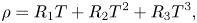
  $^{\circ }$C. In dimensional form (variables with a tilde are dimensional quantities), it is
 \begin{equation} \tilde\rho(\tilde T) = c_0 + c_1\tilde T + c_2\tilde T^{2} + c_3\tilde T^{3}. \end{equation}
The values for  $c_0$,
  $c_1$,
  $c_2$ and
  $c_3$ can be found in table 1 and values for
  $\tilde T_i$,
  $\tilde \rho (\tilde T_i)$,
  $\tilde T_a$ and
  $\tilde \rho (\tilde T_a)$ can be found in table 2.
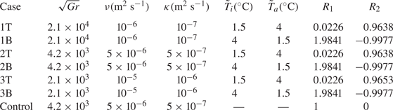
Table 1. Table of parameters held constant across all simulations. Here,  $g$ is the gravitational acceleration,
  $\rho _0$ is the constant reference density,
  $c_i$ are the constants in the equation of state,
  $H$ is the depth of the tank,
  $L$ is the length of the tank and
  $|{\rm \Delta} \rho |/ \rho _0$ is the initial dimensionless density difference for the flow.

Table 2. Outline of the cases in this study. T cases indicate cool intrusions, and B cases indicate warm intrusions. The Grashof number is defined in (2.9),  $\nu$ is the viscosity,
  $\kappa$ is the thermal diffusivity,
  $\tilde T_i$ is the intruding temperature,
  $\tilde T_a$ is the ambient temperature and
  ${R_1}$ and
  ${R_2}$ are defined in (2.5a–c). For the Control case, density is evolved directly, so intruding and ambient temperatures are not defined.

The temperature field is scaled as
 \begin{equation} T = \frac{\tilde T - \tilde T_a}{{\rm \Delta} \tilde T}, \end{equation}
with  ${\rm \Delta} \tilde T = \tilde T_i - \tilde T_a$, and the density field is scaled as
 \begin{equation} \rho = \frac{\tilde\rho - \tilde \rho(\tilde T_a)}{{\rm \Delta} \tilde \rho},\end{equation}
where  ${\rm \Delta} \tilde \rho = \tilde \rho (\tilde T_i) - \tilde \rho (\tilde T_a)$ is the initial density difference. With the scalings in (2.2) and (2.3), (2.1) can be re-cast as
 \begin{equation} \rho = {R_1}T + {R_2}T^{2} + {R_3}T^{3}, \end{equation}
where the coefficients are
 \begin{equation} {R_1} = \frac{\tilde\rho'(\tilde T_a){\rm \Delta} \tilde T}{{\rm \Delta} \tilde\rho}, \quad {R_2} = \frac{1}{2}\frac{\tilde\rho''(\tilde T_a){\rm \Delta} \tilde T^{2}}{{\rm \Delta} \tilde\rho}, \quad {R_3} = \frac{1}{6}\frac{\tilde\rho'''(\tilde T_a){\rm \Delta} \tilde T^{3}}{{\rm \Delta} \tilde\rho}.\end{equation}
Prime symbols represent derivatives with respect to temperature. Values of  ${R_1}$ and
  ${R_2}$ for each case are given in table 2 and
  ${R_3}= 0.0113$ for all cases. The scaling of density takes into account three quantities; the initial temperature difference between the intrusion and the ambient, the initial density difference between the intrusion and the ambient and the derivatives of the equation of state around the ambient temperature. Since the coefficients in the equation of state vary depending on the ambient temperature within the domain, there are different dimensionless equations of state for each type of current. For a linear equation of state,
  ${R_1} = 1$, while
  ${R_2}$ and
  ${R_3}$ are zero.
The velocity scale and time scale are
 \begin{equation} U_b = \sqrt{g'H}, \quad t_b = \sqrt{\frac{H}{g'}}, \end{equation}
where  $g' = g({|{\rm \Delta} \tilde \rho |}/{\rho _0})$ is the reduced gravity,
  $\rho _0$ is the constant reference density. These values are found in table 1. The spatial coordinates, two-dimensional velocity, time and the dynamic pressure can then be non-dimensionalized as
 \begin{equation} (x,z) = \frac{(\tilde{x},\tilde{z})}{H}, \quad (u,w) = \frac{(\tilde u,\tilde w)}{U_b},\quad t = \tilde t \sqrt{\frac{g'}{H}}, \quad p = \frac{\tilde p}{\rho_0U_b^{2}}. \end{equation}
The initial condition on the temperature field is
 \begin{equation} T = \frac{1}{2}\left(1 - \tanh\left(\frac{x - \ell}{\delta}\right)\right), \end{equation}
where  $\ell$ and
  $\delta$ are the dimensionless lock and transition lengths, which are 0.5 and 0.025 respectively. A schematic of the case with
  $\tilde T_i > \tilde T_a$ is provided in figure 1.
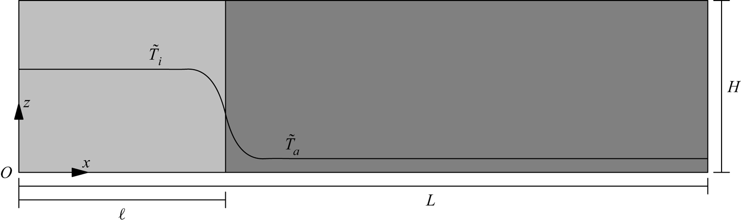
Figure 1. A schematic of the initial condition demonstrating the initial locations of  $\tilde T_i$ and
  $\tilde T_a$. In the cool intrusion cases,
  $\tilde T_i < \tilde T_a$, and in the warm intrusion cases,
  $\tilde T_i > \tilde T_a$. The lock length is given by
  $\ell$, the tank length is given by
  $L$ and the tank height is given by
  $H$. Here,
  $x$ is the horizontal coordinate,
  $z$ is the vertical coordinate and gravity points in the negative
  $z$ direction.
The scaling discussed above can be used to non-dimensionalize the incompressible Navier–Stokes equations under the Boussinesq approximation assuming a dominant balance between buoyancy and momentum diffusion. This balance can be used to define a control parameter called the Grashof number,  ${Gr}$, the form of which follows Härtel et al. (Reference Härtel, Meiburg and Necker2000b) as
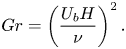 \begin{equation} {Gr} = \left(\frac{U_b H}{\nu}\right)^{2}. \end{equation}
The relative strength of momentum diffusion to temperature diffusion is kept constant across all cases and is measured by the Prandtl number,
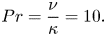 \begin{equation} Pr = \frac{\nu}{\kappa} = 10. \end{equation}
This value of the Prandtl number is representative of the value for freshwater near  $T_{md}$. In reality, the viscosity and diffusivity,
  $\nu$ and
  $\kappa$ respectively, vary weakly with temperature for the range of temperatures considered, but are kept constant for simplicity.
The equations of motion in non-dimensional form are
 \begin{gather} \frac{\textrm{D} \boldsymbol{u}}{D t} ={-}\boldsymbol{\nabla} p - \rho \hat{\boldsymbol{k}} + \frac{1}{\sqrt{{Gr}}} \nabla^{2} \boldsymbol{u}, \end{gather}
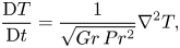 \begin{gather}\frac{\textrm{D} T}{\textrm{D} t} =\frac{1}{\sqrt{Gr\,Pr^{2}}} \nabla^{2} T, \end{gather}
 \begin{gather}\boldsymbol{\nabla} \boldsymbol{\cdot} \boldsymbol{u}= 0, \end{gather}
along with (2.4). The material derivative is represented by 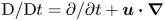 ${\textrm {D}}/{\textrm {D} t} = {\partial }/{\partial t} + \boldsymbol {u}\boldsymbol {\cdot }\boldsymbol {\nabla }$, the non-dimensional velocity by
  $\boldsymbol {u}$ (in two dimensions), time by
  $t$ and
  $\boldsymbol {k}$ represents the unit vector in the positive (upwards)
  $z$ direction.
The values for  ${Gr}$, viscosity and diffusivity are given in table 2. Case names that contain a T indicate that the gravity current is a cool intrusion (
 $\tilde T_i < \tilde T_a$) and flows along the top surface, while those with a B indicate the intrusion is a warm intrusion (
 $\tilde T_i > \tilde T_a$) and flows along the bottom surface. A control case is also included, called Control. For this case, the density field was evolved following an equation similar to (2.12), and has an equivalent driving density difference to the T and B cases. Evolving the density directly is equivalent to evolving the gravity current under a linear equation of state. All other flow parameters were unchanged for the Control case. The cases in this study were chosen to have comparable Grashof numbers of other studies such as Cantero et al. (Reference Cantero, Lee, Balachandar and Garcia2007, Reference Cantero, Balachandar, García and Bock2008) and Härtel et al. (Reference Härtel, Meiburg and Necker2000b).
2.2. Phenomenological nonlinear equation of state effects
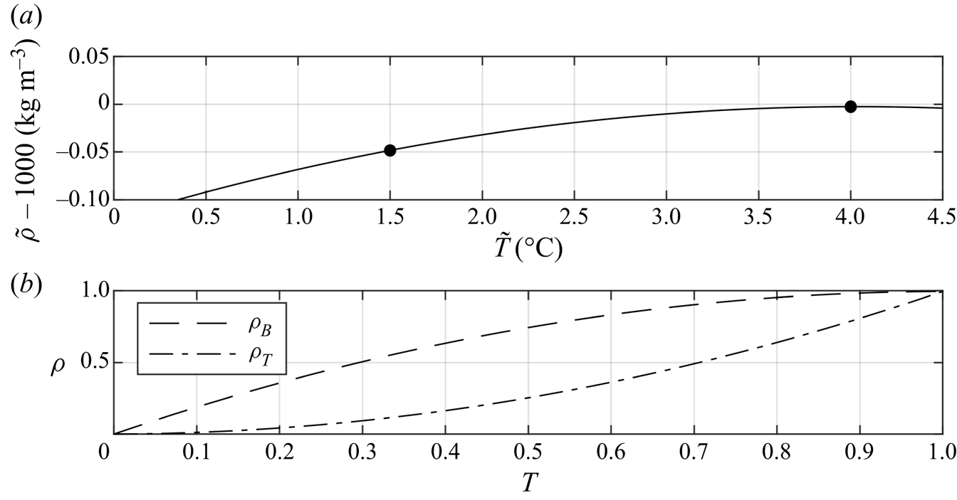
Heat is exchanged between the ambient and intrusion and their density difference will subsequently decrease assuming the temperatures reside in the monotonic cold water regime between the freezing temperature and  $T_{md}$, shown in figure 2(a). Figure 2(b) shows the dimensionless equations of state that model the density differences between the ambient and the intrusion as their temperature difference decreases. Initially, the dimensionless temperatures of both currents are
  $T = 1$. The densities of all B(T) cases are scaled such that the density–temperature relationship is given by the dashed(dot-dashed) curve, called
  $\rho _B(\rho _T)$.

Figure 2. Panel (a) shows the equation of state in the temperature regime in this study. The temperature of maximum density according to the modified equation of state, (2.1), is approximately 4  $^{\circ }$C. The black markers indicate the temperature range in this study. Panel (b) shows the scaled density–temperature relationships for each set type of current, (2.4). For the T cases, the density initially undergoes a relatively rapid change and slows as the temperature nears zero (depicted by
  $\rho _T(T)$), and vice versa for the B cases (depicted by
  $\rho _B(T)$). Note that the definition (2.3) ensures
  $\rho$ is positive.
The two different scalings reveal an important feature about this problem. The rate that the density decreases is strongly dependent on its initial configuration. For cool intruding fluid that gains heat from a much larger volume of ambient fluid at  $T_{md}$, the density will initially decrease at a relatively large rate, and as the temperature difference between the intrusion and the ambient approaches zero, the rate of decrease of the density difference will slow. Conversely, for a warm intrusion at or near
  $T_{md}$ that gives heat to the ambient, the density difference will decrease at a lower rate, until the temperature difference between the masses of water is small. At this point, the density difference begins to decrease more rapidly.
As the gravity current propagates, mixing between ambient and intruding fluids irreversibly modifies the temperature distribution within the flow. The constants in (2.4) indicate that the resulting density distributions will be different for each type of current. Insight into the relationship between temperature distributions and density distributions can be gained by first considering a test flow with normally distributed temperatures. In figure 3(a), the flow has a mean temperature of  $T = 0.4$, and in 3(b), it has a mean temperature of
  $T = 0.6$, each represented by the dark grey probability density functions (PDFs). These distributions were chosen to have standard deviations of 0.11.
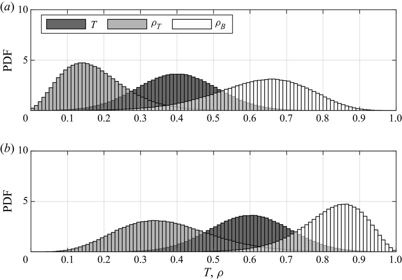
Figure 3. A conceptual demonstration of how density distributions with normally distributed temperatures depend on the dimensionless equation of state. Panel (a) shows a temperature distribution with a mean of 0.4, and panel (b) shows a temperature distribution with a mean of 0.6. Standard deviations are constant at 0.11. Refer to legend.
When temperatures are distributed such that their mean is closer to  $T = 0$ (representing the ambient temperature) than to
  $T = 1$ (representing the intruding temperature), densities described by
  $\rho _T(T)$ result in positively skewed and narrow distributions concentrated close to
  $\rho =0.15$. Conversely, densities described by
  $\rho _B(T)$ result in negatively skewed and broad distributions concentrated near
  $\rho = 0.7$. When temperatures are distributed such that their mean is closer to the intruding temperature, rather than to the ambient temperature, the opposite behaviour occurs. Thus, depending on which equation of state the flow evolves under, the density distributions within the flow are characteristically different from each other. This difference may result in large scale variation in the dynamics of the flows. Since each type of current in this study follows one of either
  $\rho _B(T)$ or
  $\rho _T(T)$, the density differences within the flow evolve in different ways. The results in the following sections demonstrate the structural and evolutionary differences that arise due to the characteristic differences between
  $\rho _B(T)$ and
  $\rho _T(T)$.
In general, temperature distributions in the simulations in this article are more complicated than the idealization in figure 3. However, normally distributed temperatures create a simple idealized model that the more complicated distributions presented in § 3 can be compared to, regardless of the exact form of the temperature distribution.
3. Simulation results
3.1. Evolution and emergent density changes
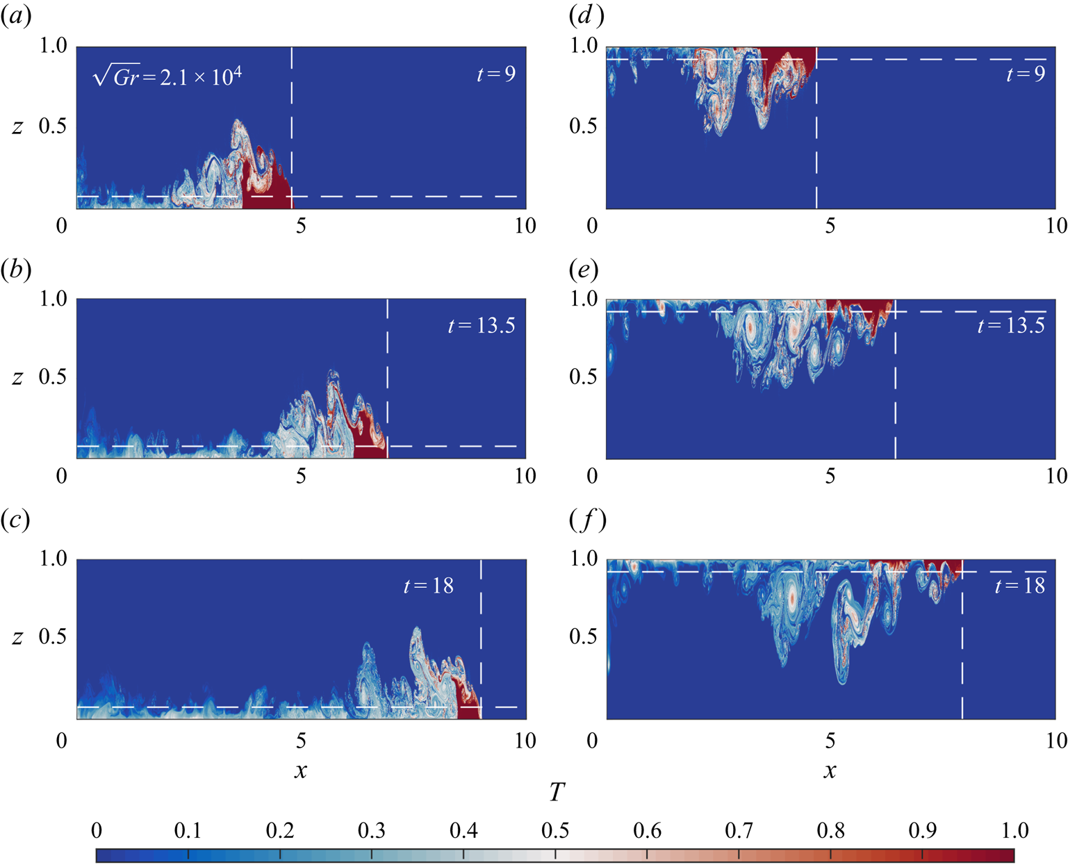
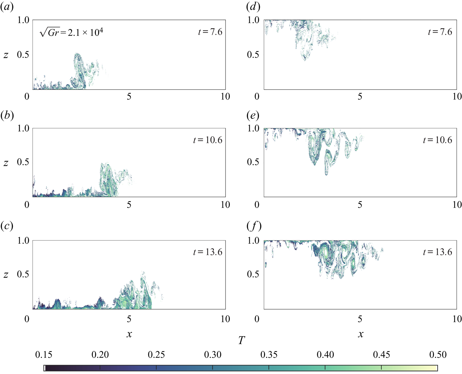
The qualitative differences between the cool and warm intrusions are noticeable from a very early stage in their development, and these differences persist as the gravity currents continue to evolve. Shown in figure 4 is the dimensionless temperature field for cases 1B in panels (a,b,c), and 1T in panels (d,e,f).

Figure 4. Temperature fields for cases 1B (a,b,c), and 1T (d,e,f). The dashed vertical lines indicate the location of the nose of the gravity current, while the dashed horizontal lines indicated the critical height where the Froude number becomes insensitive to head height (Huppert & Simpson Reference Huppert and Simpson1980).
Initially, 4(a) and 4(d) show that the gravity currents are similar in structure but by  $t = 13.5$, in (b,e), large scale differences between the two cases occur. In case 1T, vortices form in the tail of the current and intrude downwards into the water column, whereas for case 1B, much of the intruding fluid is trapped near the bottom surface, and no clear vortices form. The head of 1T is also smaller than the head of 1B. As 1T continues to propagate, small amounts of fluid are shed from the top surface and brought further into the water column ((e,f)), resulting in a much larger body than in 1B. The temperature fields of the 2B/T and 3B/T cases (not shown) have very similar structures, but the 1B/T cases show the most spatial variability because they have the largest Grashof number considered here.
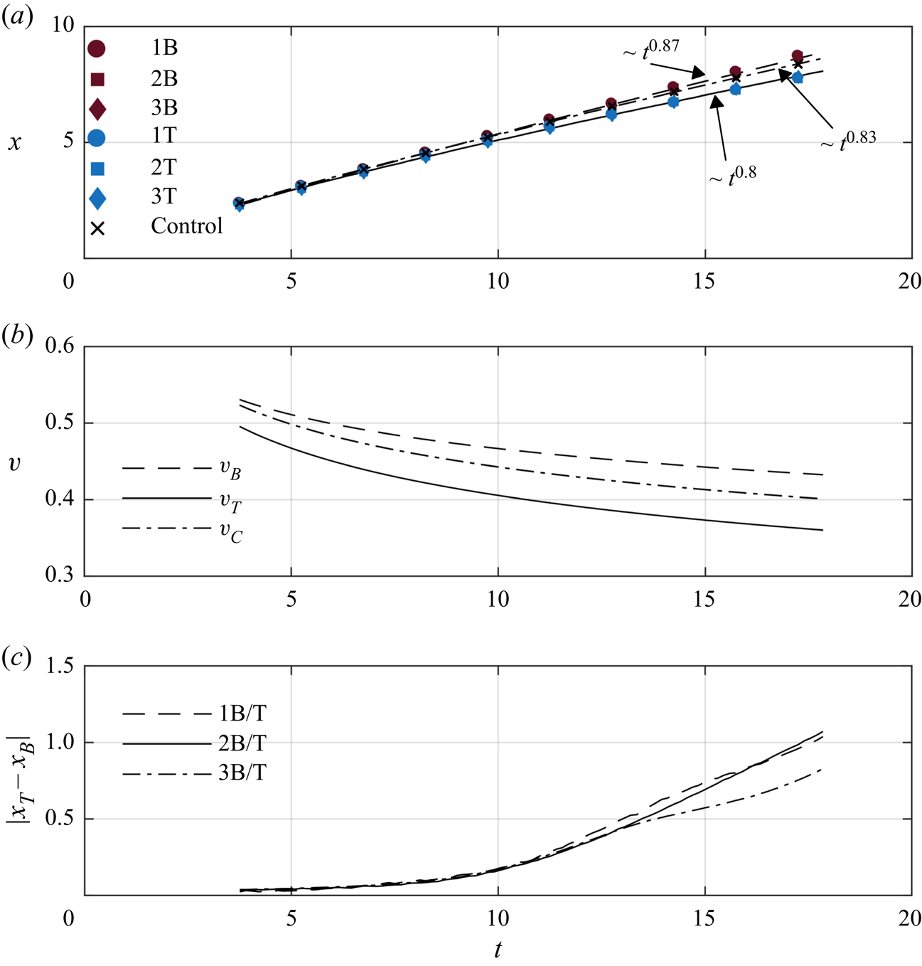
Distinct differences between the head locations occur as the currents continue to evolve. The difference is most apparent in panels (c,f), indicated by the dashed vertical lines. Comparing with the results of the 2B/T and 3B/T cases (not shown), the simulations reveal systematic differences in the head locations for all cool intrusions compared to the warm intrusions at the same  ${Gr}$. Figure 5(a) shows the head locations for all six cases with power law fits to the data, and (b) shows the non-dimensional velocity calculated from the fits. The data from the simulations are plotted as coloured markers and the fits for the B and T cases are plotted as dashed and solid lines respectively. The data were fit over an interval of
  $t \approx 4$ to
  $t \approx 18$. Cantero et al. (Reference Cantero, Balachandar, García and Bock2008) predicts that the transition between the accelerating phase and the slumping phase occurs at approximately
  $t\approx 4$, so this time was chosen as the starting point.

Figure 5. Panel (a) shows the head location of each current. Cool intrusions are denoted by blue markers and warm intrusions are denoted by red markers. The solid and dashed lines are power law fits for the cool intrusions and warm intrusions, respectively. The Control case is denoted by  $\times$ markers and the fit by the dot-dashed line. The power laws are marked on the figure. Panel (b) shows the velocity time series derived from the fits in panel (a). The solid curve is the fit for the cool intrusions,
  $v_T$, the dashed curve for the warm intrusions,
  $v_B$, and the dot-dashed line for the Control,
  $v_C$. Panel (c) shows the magnitude of the difference in the head location as a function of time between comparable cases. Cases 1B/T are denoted by the dashed line, 2B/T by the solid line and 3B/T by the dot-dashed line. Here,
  $x_T$ is the head location for cool intrusions, and
  $x_B$ is the head location of warm intrusions.
The head location for the B cases scale as  ${\sim }t^{0.87}$ across the entire time interval shown. The scaling of the B cases nearly matches the theoretical scaling of Huppert & Simpson (Reference Huppert and Simpson1980) in the slumping phase, who report that the head location scales as
  ${\sim }t^{6/7}$ as long as
  $\phi > 0.075$, where
  $\phi$ is the head height of the gravity current. This critical height is included as horizontal dashed lines in figure 4. The T cases scale as
  ${\sim } t^{0.8}$. The rate of decrease of the head height is much higher in these cases, even reaching near the critical height 0.075 by
  $t \approx 18$, which could impact the current head speed. Included in panels (a,b) are the head location and head speed for the Control case. The results show that the B cases propagate faster than the Control case while the T cases propagate slower. The rate at which the head location scales is also very similar to the slumping regime in Huppert & Simpson (Reference Huppert and Simpson1980), approximately
  ${\sim } t^{0.83}$.
Figure 5(c) shows the difference in head location for each pair of cases with the same  ${Gr}$. Here,
  $x_T$ represents the location of the T cases, and
  $x_B$ the B cases. For the 1B/T and the 2B/T cases, the curves are coincident, while the curve for 3B/T shows that the 3T case stays closer relative to the B case during the evolution. A closer examination (not shown) reveals that 3B propagates slightly slower than 1B and 2B, while the 3T moves at a rate more comparable to 1T and 2T. This indicates that decreasing the Grashof number past this threshold affects the relative disparity in the head locations. Cantero et al. (Reference Cantero, Lee, Balachandar and Garcia2007) show that gravity currents with a low Grashof number reach a viscously dominated regime much earlier in their evolution than gravity currents with higher Grashof number. Although the 3B/T cases do not formally exhibit a clear transition to this scaling regime in figure 5(a), the results from panel (c) indicate that viscosity plays a quantifiable role in the head location for those cases. Time estimates from Cantero et al. (Reference Cantero, Balachandar, García and Bock2008) suggest that the viscously dominated regime should occur near the end of the simulations for cases 3B/T, but long after the final simulation time for 1B/T and 2B/T.
Direct comparison of the two types of currents highlights the structural differences that occur as they evolve. To differentiate them further, consider the temperature PDF of case 1B in figure 6(a–g), and case 1T in figure 6(h–n). The PDFs are shown at several times between  $t = 9.1$ and
  $t = 13.6$. In each panel, the ambient temperature is in the left most bin, while the intruding temperature is in the right most bin. At
  $t = 0$, the distribution of temperature is bimodal, with one peak located at the ambient temperature and one peak located at the intruding temperature. The volume of the ambient fluid in both the B and T cases is much larger than the volume of intruding fluid. Thus, the PDFs show a bias towards the ambient temperature throughout figure 6. At
  $t = 9.1$, the PDFs reveal that a broad distribution of intermediate temperatures form because of mixing of ambient and intruding fluids. By
  $t = 13.6$, the distributions evolve and form peaks centred around
  $T= 0.38$ in 1B and around
  $T = 0.3$ in 1T. The peak in 1B is more well defined than in 1T, indicating a wider distribution of temperatures and suggesting more mixing in the latter case. In both cases, there is a much lower probability of finding temperatures between approximately 0.6 and 0.95 within the domain.
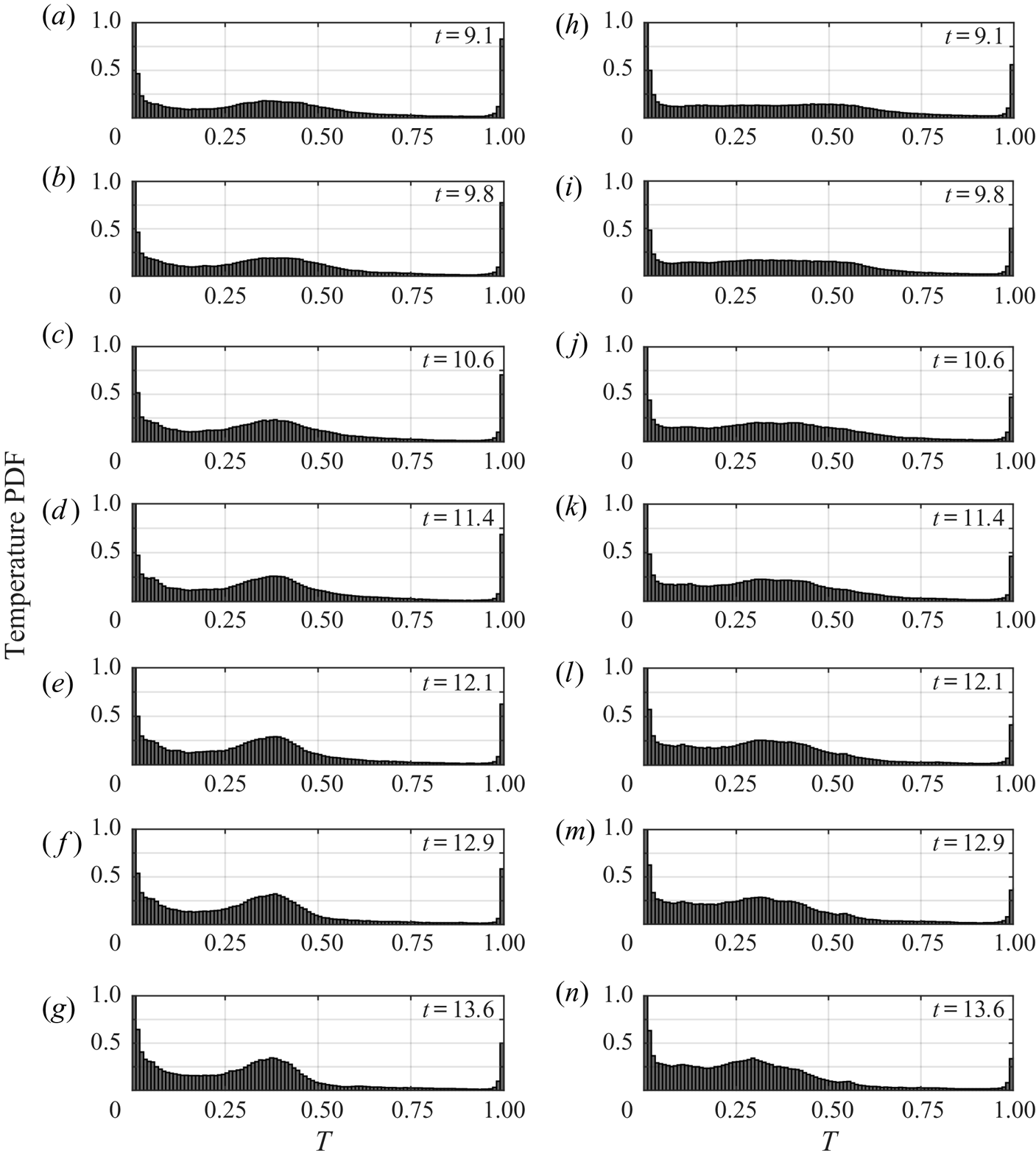
Figure 6. PDFs of the non-dimensional temperature for cases 1B (a–g) and 1T (h–n) at successive time intervals, indicated on the plots. The bin width is 0.01, and the vertical axis is capped at 1 to avoid clouding the data. The ambient temperature is located within the left most bin, and the intruding temperature is within the right most bin.
The regions with temperatures between  $T = 0.15$ and
  $T = 0.5$ (approximately surrounding the peaks in the PDFs in figure 6(h,n) where mixing has occurred) in the gravity currents are plotted in figure 7. The peak in the intermediate temperatures in the PDFs approximately corresponds to the tail region of the gravity current, with the head being primarily outside this region. It is the tail region where ambient fluid is rapidly mixed with intruding fluid that forms the peak in the PDFs.

Figure 7. Regions of the gravity current where the non-dimensional temperature field varies between  $T = 0.15$ and
  $T= 0.5$. Case 1B is shown in panels (a–c), and 1T in panels (d–f). Times of the plots are on each panel.
The density PDFs for case 1B are shown in figure 8(a–g) and case 1T is shown in figure 8(h–n) at the same times as the corresponding temperature PDFs shown in figure 6. In each panel, the ambient density is in the left most bin, while the intruding density is in the right most bin. Figure 8 reveals the wide variations of the density distribution within the two currents. At  $t = 9.1$, the density distribution for 1B is broad with a small peak at approximately
  $\rho = 0.6$, but for 1T no such peak exists and the range of densities in the domain are much closer to the ambient. This is a clear indication of how the nonlinear equation of state strongly affects the density distributions of the two currents. By
  $t = 13.6$, the density PDF for 1B has a clear peak (the tail of the current), while the PDF for 1T shows something completely different.
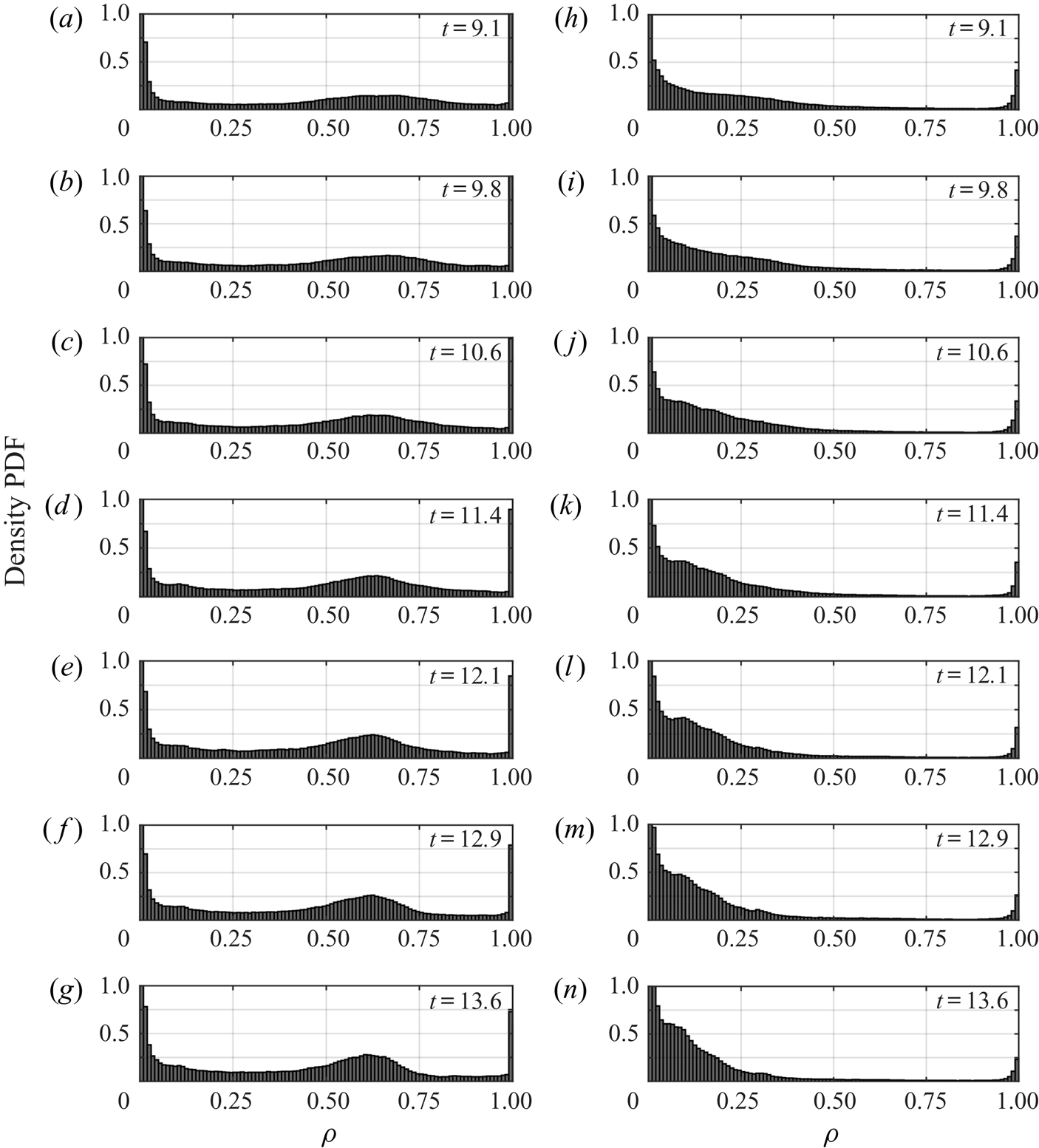
Figure 8. PDFs of the density for cases 1B (a–g) and 1T (h–n) at successive time intervals, indicated on the plots. The bin width is 0.01, and the vertical axis is capped at 1 to avoid clouding the data. The ambient density is located within the left most bin, and the intruding density is within the rightmost bin.
Figure 9 shows the densities of the regions depicted in figure 7. The temperature bounds used in figure 7 translate to approximately  $\rho = 0.05$ and
  $\rho = 0.25$ for 1T (figure 9a–c) and approximately
  $\rho = 0.25$ to
  $\rho = 0.75$ for 1B (figure 9d–f). The most obvious consequence of the nonlinear equation of state is the difference between the densities in the tail of each type of current. For 1B, as fluid travels toward the tail of the current, it mixes with some ambient fluid resulting in a relative density of approximately 0.6, and the buoyancy force on this fluid is strong enough to draw it back into the current. As fluid travels towards the tail in the 1T case, it mixes with ambient fluid and achieves a relative density that nearly matches the ambient. The buoyancy force on this fluid is not nearly as strong, and this leads to a larger tail.
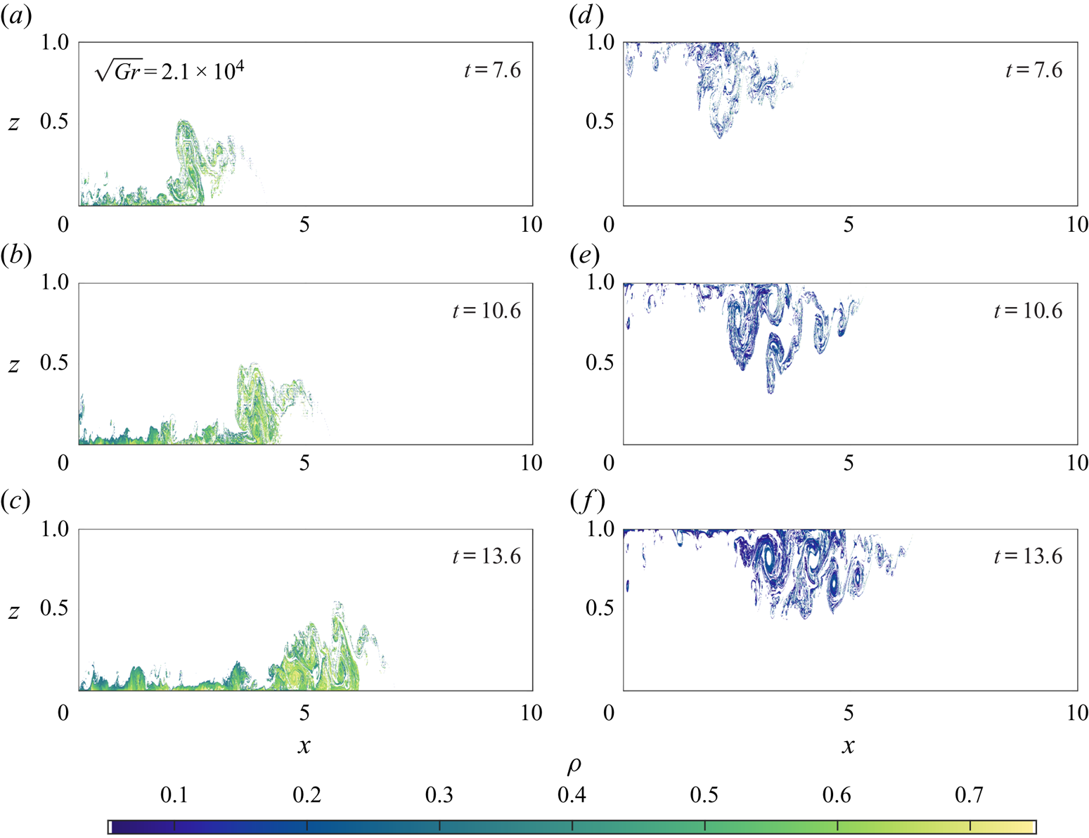
Figure 9. The non-dimensional density of the current in the regions coinciding with those shown in figure 7. Case 1B is shown in panels (a–c), and case 1T is shown in panels (d–f). Times of the plots are on each panel.
An analogy to figure 3 can be made. As the fluid in the tail region is mixed over the course of the evolution of the current, the temperature distribution is seen to form a peak. As the peak becomes more well defined and closer to the ambient temperature, the density distributions for each category of current are affected asymmetrically. The warm intrusions flatten and with the mean closer to the intruding density, similar to what develops in figure 8(a–g). The cool intrusions form a peak that is close enough to the ambient density that it blends with the temperatures in that part of the distribution. This behaviour is not unlike the idealization in figure 3(a), although it is clouded by the vast amount of ambient fluid, especially for the 1T case. However, as a simple model, it serves the purpose of explaining why there is a stark contrast between the density fields of the evolving currents.
To summarize the main findings above, an empirical formulation of the density of the current as a function of its temperature can be determined by defining the phenomenological current temperature following Cantero et al. (Reference Cantero, Balachandar, García and Bock2008). An indicator function is defined as
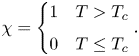 \begin{equation} \chi = \begin{cases} 1 & T > T_c \\ 0 & T \leq T_c \end{cases}. \end{equation}
The average temperature of the intrusion is denoted
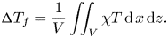 \begin{equation} {\rm \Delta} T_f = \frac{1}{V}\iint_V \chi T \, \mathrm{d}\kern1.5pt x\,\mathrm{d}z. \end{equation}
The average temperature of the intrusion is the average temperature of the region of the flow where the temperatures are greater than a cutoff temperature. The cutoff used here is  $T_c = 0.01$, which corresponds to all temperatures to the right of the left most bin in all panels of figure 6. The critical temperature corresponds to
  $\tilde T = 1.525\,^{\circ }$C for the T cases and
  $\tilde T = 3.975\,^{\circ }$C for the B cases. These temperatures characterize the currents very well. The average density is defined in a similar way,
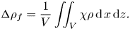 \begin{equation} {\rm \Delta} \rho_f = \frac{1}{V}\iint_V \chi\rho \,\mathrm{d}\kern1.5pt x\,\mathrm{d}z. \end{equation}
Note that there is an important distinction to be made in this temperature regime. The average density is not equal to the density of the average temperature as it would be under a linear equation of state, so  ${\rm \Delta} \rho _f$ cannot be defined as the
  $\rho ({\rm \Delta} T_f)$.
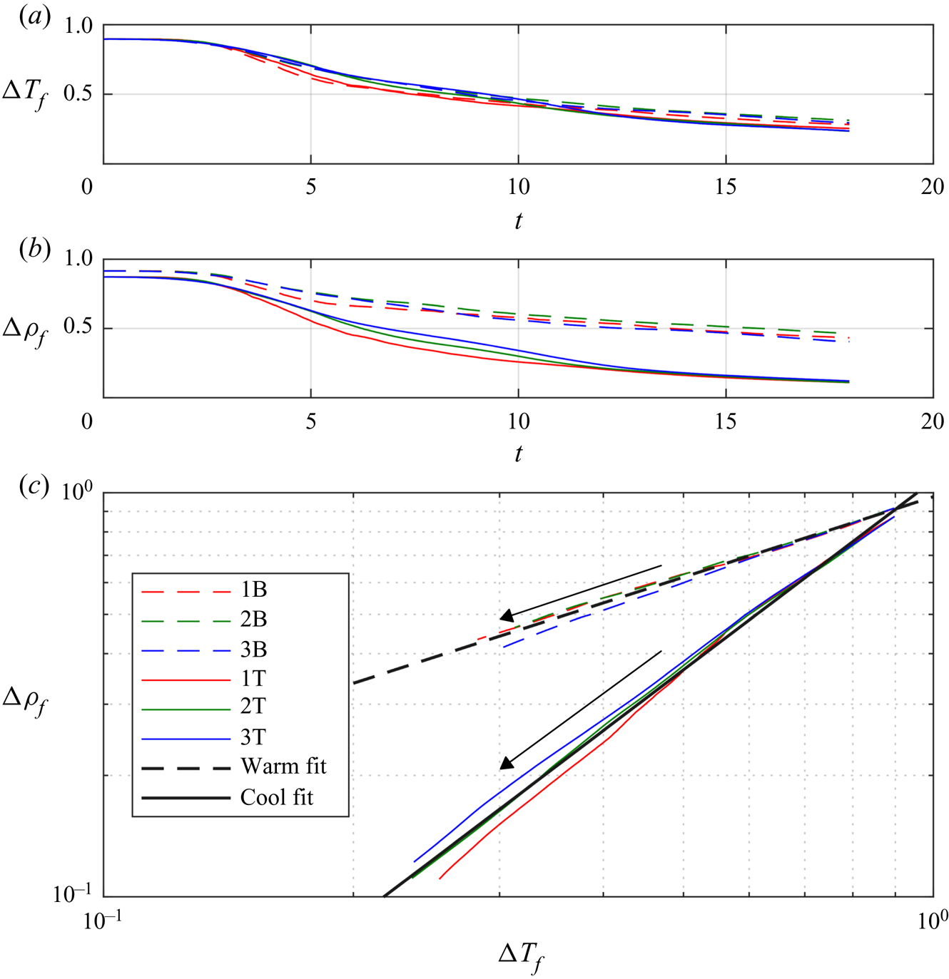
Plotted in figure 10(a) is the average temperature of the current. For all cases, the decrease in  ${\rm \Delta} T_f$ follows the same trend, but cases 1B and 1T appears to decrease slightly faster, due to the large
  ${Gr}$. The basic result is that the temperature difference between the ambient and the intrusion does not significantly discriminate between the cool intrusion and warm intrusion across all values of
  ${Gr}$. Figure 10(b) shows the average density of the current. It is clear from this plot that the density difference is dependent on whether the intrusion is gaining heat or losing heat, as
  ${\rm \Delta} \rho _f$ is smaller for the cool intrusion than for the warm intrusion for
  $t \gtrsim 6$. This is qualitatively consistent with the hypothesis discussed above (see figure 2(b) and related discussion). Shown in panel (c) is the average temperature of the current plotted against the average density. The average density of the current follows the power law
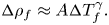 \begin{equation} {\rm \Delta} \rho_f \approx A{\rm \Delta} T_f^{\gamma}. \end{equation}
For the cool intrusions,  $A \approx 1.07$ and
  $\gamma \approx 1.57$, while for the warm intrusions
  $A \approx 0.97$ and
  $\gamma \approx 0.67$.

Figure 10. Panel (a) shows  ${\rm \Delta} T_f$ data for all cases. Panel (b) shows
  ${\rm \Delta} \rho _f$ data for all cases. Panel (c) shows
  ${\rm \Delta} \rho _f$ plotted against
  ${\rm \Delta} T_f$ for all cases. Warm intrusions are given by dashed lines and the cool intrusions by solid lines. Fits for each set of currents (warm and cool) are included on the plot. The direction of time for each set of cases in panel (c) is indicated by the arrows.
The constant  $\gamma$ describes the rate at which the average density of the current changes as its average temperature changes. Figure 10 demonstrates that the change in density is higher for a given temperature change for the cool intrusion (
 $\gamma = 1.53$) than it is for the warm intrusion (
 $\gamma = 0.67$). There is some spread in the data, especially when the temperature differences become small, however, this relationship characterizes the difference between the cool intrusions and warm intrusions well.
4. Discussion
4.1. Implications for gravity current evolution
This study presents numerical simulations of two categories of gravity currents in the cold water regime (temperatures less than  $T_{md}$). Differences between the categories arise due to the way the fluid density changes as heat is transferred between the intruding and ambient fluids. Warm intrusions near at
  $4\,^{\circ }$C undergo a gradual change in density, leading to structures more reminiscent of a traditional gravity current. Cool intrusions at
  $1.5\,^{\circ }$C undergo an initial rapid change in density, and exhibit more fluid being torn from the current, resulting in a qualitatively different body shape and a much smaller head. It is important to note that gravity currents will behave in a similar way when temperatures are greater than
  $T_{md}$, but close enough that the equation of state is still nonlinear.
A consistent feature demonstrated by the numerical experiments is a clear difference in the location of the head of the cool intrusions with respect to the warm intrusions after enough time has elapsed. The head locations for the B and T cases scale differently than each other, and different also to the Control case that uses a linear equation of state. A single power law for each set of cases is adequate to describe this difference. In none of the cases does the head speed exhibit a clear transition from the slumping regime to the inertial regime, as suggested by Huppert & Simpson (Reference Huppert and Simpson1980) and Cantero et al. (Reference Cantero, Lee, Balachandar and Garcia2007, Reference Cantero, Balachandar, García and Bock2008), even though both the volume of intruding fluid and Grashof number were comparable to the cases of Härtel et al. (Reference Härtel, Meiburg and Necker2000b), Cantero et al. (Reference Cantero, Balachandar, García and Bock2008) and some of the experiments of Huppert & Simpson (Reference Huppert and Simpson1980). The closest approximation to the established scaling laws are the B cases and the Control case having scaling laws close to  ${\sim }t^{6/7}$, which is what Huppert & Simpson (Reference Huppert and Simpson1980) found to characterize the slumping regime. The lack of agreement between the head location of the Control case with the established scaling laws could be a result of the slip boundaries used in this article. Härtel et al. (Reference Härtel, Meiburg and Necker2000b) discusses effects of no-slip boundaries versus slip boundaries, but does not discuss in detail how the head location differs as the boundary conditions are changed.
The difference in the scaling laws occurs because the nonlinear relationship between the driving density difference and the evolving temperature differences affects the evolution of the current in different ways. In the linear regime of the freshwater equation of state, the rate that the density of the current changes is independent of the exact temperatures of the current and the ambient, and is only dependent on their difference. However, in the cold water regime, the temperatures of the ambient and the intrusion play a role in how the density will change as the fluids of different temperatures are mixed, depicted graphically in figure 2(b), and mathematically by the ambient temperature dependence of  ${R_1}$ and
  ${R_2}$ (with the cubic equation of state,
  ${R_3}$ remains unchanged for both kinds of currents).
The simulation results above show that, at high Grashof number, the temperature distributions of the two types of currents are initially broadly distributed and tend to sharpen as the current mixes in the tail region, resulting in similar temperature distributions for the 1B and 1T cases. The peak of the temperature distribution tends to be closer to the ambient temperature than intruding temperatures in both cases near the end of the simulations. Figure 3 suggests that when the temperature distribution is closer to the ambient temperature, currents that follow  $\rho _T(T)$ (the T cases) will have sharper density distributions that tend to be close to the ambient density while currents that follow
  $\rho _B(T)$ (the B cases) will have flatter density distributions that tend to be closer to the intruding density. The general trend from the simulations agrees with this. For the T cases, as fluid rolls up on the interface between the current and the ambient, it mixes near the tail and attains a density close enough to the ambient that its motion nearly ceases. The net effect is a large tail reaching deep into the water column. Comparatively, the B cases look more like a traditional gravity current because as fluid rolls up and mixes, the density achieved is still far enough away from that of the ambient that there is still a significant downward buoyant force that returns it into the current.
4.2. Insights for cabbeling in shallow bodies of water
Density driven flows in this temperature regime have been previously shown to exhibit downward biases because of the nonlinearity in the equation of state. Olsthoorn et al. (Reference Olsthoorn, Tedford and Lawrence2019) showed that downward growing plumes had larger length scales and grew faster than upward growing plumes in numerical simulations of finite thickness Rayleigh–Taylor instabilities. Ozgökmen & Esenkov (Reference Ozgökmen and Esenkov1998) demonstrated the same behaviour in the growth of salt fingers. This downward bias is related to the phenomenon known as cabbeling, and the results of this study provides insight into how cabbeling could impact the vertical dispersion of intruding fluid in the fresh cold water regime.
Traditionally, cabbeling refers to how two fluid parcels of equal density but different temperatures mix to create a parcel that is denser than both parents (McDougall Reference McDougall1987). The cold water regime precludes mixing between fluid parcels with equal density and different temperatures due to the monotonicity of the equation of state, so a more apt definition provided by Stewart et al. (Reference Stewart, Haine, McHogg and Roquet2017) relates cabbeling to the process of mixing two water masses at different temperatures and forming a mass that is denser than the average of the source densities.
Where cabbeling traditionally generates downward fluxes of momentum and heat due to the formation of dense water (Thomas & Shakespeare Reference Thomas and Shakespeare2015; Shakespeare & Thomas Reference Shakespeare and Thomas2017), the net effect of cabbeling in the cold water regime, termed ‘weak cabbeling’, is to enhance pre-existing downward fluxes of intruding fluid, and to weaken upward fluxes. The results in figure 4 demonstrate that for cool intrusions, fine filament structures reach far deeper into the water column, while for the warm intrusions, intruding fluid is confined closer to the bottom surface, unable to rise further up into the water column. This behaviour is in qualitative agreement with the results of both Olsthoorn et al. (Reference Olsthoorn, Tedford and Lawrence2019) and Ozgökmen & Esenkov (Reference Ozgökmen and Esenkov1998).
The results of this paper show that the subtle example of cabbeling created in the cold water regime can have clear impacts on the small scale non-hydrostatic dynamics of gravity currents. Weak cabbeling may even have implications for the vertical fluxes of material at the surface or bottom of a lake, especially near a river outflow, where masses of water are rapidly mixed.
Acknowledgements
The authors would like to thank the three anonymous reviewers whose suggestions have led to substantial improvements to this paper.
Funding
This work was supported by a grant from Global Water Futures, funded by the Canada First Research Excellence Fund and from the Canadian Foundation for Innovation and the Ontario Research Fund.
Declaration of interest
The authors report no conflict of interest.