


1. Introduction
Convection driven by buoyancy is abundant in geophysical and astrophysical flows, from atmospheric convection driving ocean currents to solar convection transporting heat in stars. The prototypical set-up for studying these flows is that of Rayleigh–Bénard convection, where flow in a layer of fluid is driven by the temperature differential across the boundaries. In reality, convection in many natural or engineering situations is at least partially driven by an internal heating source. Examples include convection in the Earth's mantle due to radiogenic heat (Davies & Richards Reference Davies and Richards1992; Schubert, Turcotte & Olson Reference Schubert, Turcotte and Olson2001; Mulyukova & Bercovici Reference Mulyukova and Bercovici2020), convection in radiative planet atmospheres (Pierrehumbert Reference Pierrehumbert2010; Seager Reference Seager2010; Guervilly, Cardin & Schaeffer Reference Guervilly, Cardin and Schaeffer2019), and engineering flows where exothermic chemical or nuclear reactions drive the convection (Tran & Dinh Reference Tran and Dinh2009). Gaining insights into these physical and practical scenarios requires a thorough understanding of internally heated (IH) convection, yet studies in this direction are relatively few.
Following the early investigations by Roberts (Reference Roberts1967) and Tritton (Reference Tritton1975), recently research into IH convection has gained renewed momentum through computational analysis (Goluskin & Spiegel Reference Goluskin and Spiegel2012; Goluskin Reference Goluskin2015; Goluskin & van der Poel Reference Goluskin and van der Poel2016) and experiments (Lepot, Aumaître & Gallet Reference Lepot, Aumaître and Gallet2018; Bouillaut et al. Reference Bouillaut, Lepot, Aumaître and Gallet2019; Limare et al. Reference Limare, Jaupart, Kaminski, Fourel and Farnetani2019, Reference Limare, Kenda, Kaminski, Surducan, Surducan and Neamtu2021). However, a comprehensive understanding of flows driven by internal heating is far from complete, and the behaviour of such flows in the limiting regime of extreme heating remains unknown.
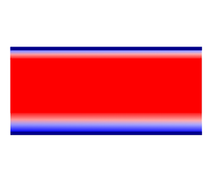
Here, we probe this regime using rigorous upper bounding theory. Specifically, we bound the mean vertical convective heat flux in two configurations of IH convection, one where the fluid is bounded between horizontal plates held at the same temperature, and one where the bottom plate is replaced by a perfect insulator. These two configurations, which we refer to as IH1 and IH3 following the terminology introduced by Goluskin (Reference Goluskin2016), are illustrated schematically in figure 1(a,b).

Figure 1. The two configurations considered in this paper. (a) IH1: isothermal boundaries. (b) IH3: isothermal top boundary and insulating bottom boundary. In both configurations, the heating is uniform, so the non-dimensional thermal source term is  $H = 1$. Dashed lines show the temperature profiles in the pure conduction state, while solid lines sketch the temporally- and horizontally-averaged temperature profiles in a typical turbulent state (also shown using the colour plot).
The mean vertical convective heat flux  $\langle wT \rangle$, where
  $w$ and
  $T$ are the non-dimensional vertical velocity and temperature, and angle brackets denote space–time averages, has a slightly different physical interpretation in the two configurations. For the IH1 case,
  $\langle w T \rangle$ is related to the asymmetry in the heat fluxes
  $\mathcal {F}_T$ and
  $\mathcal {F}_B$ through the top and the bottom boundaries. Specifically, space–time averaging the dimensionless transport equation for temperature (see (2.1c) in § 2) multiplied by the wall-normal coordinate
  $z$ yields
 \begin{equation} \mathcal{F}_T = \tfrac{1}{2} + \langle w T \rangle, \quad \mathcal{F}_B = \tfrac{1}{2} - \langle w T \rangle. \end{equation}
In the purely conductive state, the heat generated inside the domain leaves equally between the two boundaries, hence  $\mathcal {F}_T = \mathcal {F}_B = 1/2$. In the convective state, instead, the asymmetry of buoyancy combines with the uniform heat source to create boundary layers with different characteristics near the top and bottom boundaries, as illustrated in figure 1(a). The bottom boundary layer is stably stratified, whereas the top boundary layer is unstably stratified. Convective heat transport (
 $\langle wT\rangle > 0$) makes the top boundary layer thinner than the bottom one, so in any convective state one has
  $\mathcal {F}_T > \mathcal {F}_B$. Since the boundary temperature is fixed and the fluid is internally heated, one also expects the boundary flux
  $\mathcal {F}_B$ to remain non-negative, meaning that heat can escape from the bottom boundary but not enter through it. This fact can be proved rigorously (Goluskin & Spiegel Reference Goluskin and Spiegel2012, Appendix A.1; Arslan et al. Reference Arslan, Fantuzzi, Craske and Wynn2021b, Appendix A) and translates into the following upper bounds on the vertical heat transport (Goluskin & Spiegel Reference Goluskin and Spiegel2012):
 \begin{equation} \langle w T \rangle \leq \tfrac{1}{2} \quad \text{in IH1}.\end{equation}
 For the IH3 configuration, instead, the mean vertical flux  $\langle w T \rangle$ is related to the difference of the horizontally-averaged temperature between the top
  $\bar {T}_T$ and the bottom wall
  $\bar {T}_B$. Indeed, upon multiplying the dimensionless evolution equation for the temperature (see (2.1c) in § 2) with the wall-normal coordinate
  $z$ and space–time averaging, one obtains
 \begin{equation} \langle w T \rangle = \bar{T}_T -\bar{T}_B + \tfrac12. \end{equation}
The isothermal boundary condition implies that the temperature  $T_T$ at the top boundary is in fact constant, so
  $\bar {T}_T = T_T$, and we take it as zero without loss of generality in our non-dimensionalization. Since the non-dimensional internal heating rate is positive, one expects the mean bottom temperature
  $\bar {T}_B$ to be non-negative. As before, this fact can be proved rigorously and results in the upper bound (Goluskin Reference Goluskin2016, Chapter 1)
 \begin{equation} \langle w T \rangle \leq \tfrac{1}{2}\quad \text{in IH3}.\end{equation}
 For the IH1 configuration, Arslan et al. (Reference Arslan, Fantuzzi, Craske and Wynn2021b) proved recently that  $\langle w T \rangle \leq 2^{-21/5}R^{1/5}$, where
  $R$ is a non-dimensional parameter that measures the strength of the internal heating and may be interpreted as a Rayleigh number. This result, which is independent of the Prandtl number
  $Pr$, fails to improve the uniform bound in (1.2) for
  $R > 2^{16}=65\ 536$. However, numerical evidence by the same authors suggests that an upper bound on
  $\langle w T \rangle$ approaching
  $1/2$ from below monotonically as
  $R$ is increased may be provable when the background method by Doering & Constantin (Reference Doering and Constantin1992, Reference Doering and Constantin1994, Reference Doering and Constantin1996) and Constantin & Doering (Reference Constantin and Doering1995) is augmented with a minimum principle stating that the fluid's temperature cannot be smaller than that at the top boundary. Unfortunately, they also provided a rather tantalizing proof that such a bound cannot be obtained using typical analytical constructions.
In this paper we overcome this barrier and show that  $R$-dependent bounds on
  $\langle wT \rangle$ strictly smaller than
  $1/2$ can be obtained analytically not only in the IH1 case, but also for the IH3 configuration. Precisely, we prove that
 $$\begin{gather} \langle w T \rangle \leq \tfrac{1}{2} - c_1 R^{{1}/{5}} \exp ({-}c_2 R^{{3}/{5}}) \quad \text{in IH1}, \end{gather}$$
 $$\begin{gather}\langle w T \rangle \leq \frac{1}{2} - \frac{c_3}{R^{{1}/{5}}} \exp ({-}c_4 R^{{3}/{5}}) \quad \text{in IH3}, \end{gather}$$
where  $c_1$,
  $c_2$,
  $c_3$ and
  $c_4$ are constants (independent of both
  $R$ and
  $Pr$). To establish these results, we formulate a bounding principle for
  $\langle wT \rangle$ using the auxiliary functional method (Chernyshenko et al. Reference Chernyshenko, Goulart, Huang and Papachristodoulou2014; Fantuzzi et al. Reference Fantuzzi, Goluskin, Huang and Chernyshenko2016; Chernyshenko Reference Chernyshenko2017; Tobasco, Goluskin & Doering Reference Tobasco, Goluskin and Doering2018). This method is a generalization of the background method of Doering and Constantin, which has been applied successfully to several fluid dynamical problems (Doering & Constantin Reference Doering and Constantin1992, Reference Doering and Constantin1996; Constantin & Doering Reference Constantin and Doering1995; Caulfield & Kerswell Reference Caulfield and Kerswell2001; Tang, Caulfield & Young Reference Tang, Caulfield and Young2004; Whitehead & Doering Reference Whitehead and Doering2011b; Goluskin & Doering Reference Goluskin and Doering2016; Fantuzzi Reference Fantuzzi2018; Fantuzzi, Pershin & Wynn Reference Fantuzzi, Pershin and Wynn2018; Kumar Reference Kumar2020, Reference Kumar2022; Kumar & Garaud Reference Kumar and Garaud2020; Arslan et al. Reference Arslan, Fantuzzi, Craske and Wynn2021a,Reference Arslan, Fantuzzi, Craske and Wynnb; Fan, Jolly & Pakzad Reference Fan, Jolly and Pakzad2021). The auxiliary functional method, as implemented in this paper, also has an equivalent formulation using the background method.
The novelty aspects in our arguments are the use of a background temperature field with a lower boundary layer growing as  $z^{-1}$, motivated by the numerical results of Arslan et al. (Reference Arslan, Fantuzzi, Craske and Wynn2021b), and the application of Hardy inequalities (IH1) and Rellich inequalities (IH3). Such inequalities have already been employed to prove bounds on convective flows at infinite Prandtl number (Doering, Otto & Reznikoff Reference Doering, Otto and Reznikoff2006; Whitehead & Doering Reference Whitehead and Doering2011a), but to the best of our knowledge, their use at finite Prandtl number is new.
The rest of this work is organized as follows. We start by describing the problem set-up in § 2. In § 3, we apply the auxiliary function method to formulate upper bounding principles for  $\langle wT \rangle$ in both IH1 and IH3 configurations. We then prove the upper bound (1.5a) in § 4 and the upper bound (1.5b) in § 5. Finally, § 6 discusses our method of proof, compares our results with available phenomenological theories, and offers concluding remarks.
2. Problem set-up
We consider the flow of a Newtonian fluid of density  $\rho$, viscosity
  $\nu$, thermal diffusivity
  $\kappa$, and specific heat capacity
  $c_p$, driven by buoyancy forces resulting from internal heating. The fluid is confined between two horizontal no-slip plates with a gap of width
  $d$, and the heat is produced at a constant volumetric rate of
  $H^\ast$ (with units
  $\mathrm {W\ m}^{-3}=\mathrm {kg\ ms}^{-3}$). We consider the two configurations sketched in figure 1, one where both plates are kept at constant temperature
  $T_0^\ast$ (IH1) and one where the top plate is kept at a constant temperature
  $T_0^\ast$ while the bottom plate is insulating (IH3). We assume that the fluid properties are a weak function of the temperature, and use the Naiver–Stokes equations under the Boussinesq approximation to model the problem. Various justifications have been put forward for the Boussinesq approximation; see, for example, Spiegel & Veronis (Reference Spiegel and Veronis1960) and Rajagopal, Ruzicka & Srinivasa (Reference Rajagopal, Ruzicka and Srinivasa1996). In their non-dimensional form, the governing equations are
 $$\begin{gather} \boldsymbol{\nabla} \boldsymbol{\cdot} \boldsymbol{u} = 0, \end{gather}$$
 $$\begin{gather}\partial_t \boldsymbol{u} + \boldsymbol{u} \boldsymbol{\cdot} \boldsymbol{\nabla} \boldsymbol{u}+ \boldsymbol{\nabla} p = Pr\,\nabla^2 \boldsymbol{u} + Pr\,R T \boldsymbol{e}_z, \end{gather}$$
 $$\begin{gather}\partial_t T + \boldsymbol{u} \boldsymbol{\cdot} \boldsymbol{\nabla} T = \boldsymbol{\nabla}^2 T + 1, \end{gather}$$
where we have used the following non-dimensionalization for the variables:
 \begin{equation} \boldsymbol{x} = \frac{\boldsymbol{x}^\ast}{d}, \quad t = \frac{t^\ast}{d^2/ \kappa}, \quad \boldsymbol{u} = \frac{\boldsymbol{u}^\ast}{\kappa/d}, \quad p = \frac{p^\ast{-} p_0}{\rho \kappa^2/d^2}, \quad T = \frac{T^\ast{-} T_0^\ast}{d^2 H^\ast{/} (\kappa \rho c_p)}. \end{equation}
Here,  $\boldsymbol {x}$,
  $t$,
$t$,  $\boldsymbol {u}$,
  $p$ and
  $T$ denote the non-dimensional position, time, velocity, pressure and temperature, respectively, whereas
  $p_0$ is the dimensional hydrostatic ambient pressure. The quantities with a star superscript are dimensional. The non-dimensional governing parameters of the flow are the Prandtl number and the Rayleigh number, given by
 \begin{equation} Pr = \frac{\nu}{\kappa} \quad\text{and}\quad R = \frac{g \alpha d^5 H^\ast}{\rho c_p \nu \kappa^2}, \end{equation}
where  $\alpha$ is the coefficient of thermal expansion. Our choice of non-dimensionalization implies that the heating source appears as a unit force in (2.1c).
We use the Cartesian coordinates  $\boldsymbol {x} = (x, y, z)$ and place the origin of the coordinate system at the bottom plate. The
  $z$ direction points vertically upwards, and the
  $x$ and
  $y$ directions are horizontal. In this coordinate system, we write the velocity vector as
  $\boldsymbol {u} = (u, v, w)$, where
  $u$,
$u$,  $v$ and
  $w$ are the velocity components in the
  $x$,
$x$,  $y$ and
  $z$ directions, respectively. In this coordinate system, the boundary conditions at the top and bottom plates for velocity and temperature can be written as
 $$\begin{gather} \boldsymbol{u}(x, y, 0, t) = \boldsymbol{u}(x, y, 1, t) = \boldsymbol{0}, \end{gather}$$
 $$\begin{gather}T(x, y, 0, t) = T(x, y, 1, t) = 0 \quad \text{for IH1,} \end{gather}$$
 $$\begin{gather}\partial_z T(x, y, 0, t) = T(x, y, 1, t) = 0 \quad \text{for IH3.} \end{gather}$$
We further assume that the fluid layer is periodic in the horizontal directions  $x$ and
  $y$ with lengths
  $L_x$ and
  $L_y$, meaning that the domain of interest is
  $\varOmega = \mathbb {T}_{[0, L_x]} \times \mathbb {T}_{[0, L_y]} \times [0, 1]$.
Throughout the paper, spatial averages, long-time horizontal averages and long-time volume averages will be denoted, respectively, by
 $$\begin{gather} {\int\hskip -1,05em -\,}_{\varOmega} [{\cdot} ]\,{\rm d}\boldsymbol{x} = \frac{1}{L_x L_y} \int_{0}^{1} \int_{0}^{L_y} \int_{0}^{L_x} [{\cdot} ] \, \textrm{d}\kern0.06em x \, \textrm{d} y \, \textrm{d}z, \end{gather}$$
 $$\begin{gather}\overline{[{\cdot} ]} = \lim_{\tau \to \infty} \frac{1}{\tau L_x L_y} \int_{0}^\tau \int_{0}^{L_y} \int_{0}^{L_x} [{\cdot} ] \, \textrm{d}\kern0.06em x \, \textrm{d} y \, \textrm{d}t, \end{gather}$$
 $$\begin{gather}\langle[{\cdot} ]\rangle = \lim_{\tau \to \infty} \frac{1}{\tau} \int_{0}^\tau {\int\hskip -1,05em -\,}_{\varOmega} [{\cdot} ] \, \textrm{d}\boldsymbol{x} \, \textrm{d}t. \end{gather}$$
3. The auxiliary functional method
A bound on the mean vertical heat flux can be derived using the auxiliary function method. The formulation of the method given here is very similar to the one given by Arslan et al. (Reference Arslan, Fantuzzi, Craske and Wynn2021b) for isothermal boundaries, but we repeat it to make the paper self-contained and highlight the changes required when the lower boundary is insulating.
Let  $\mathcal {V}\{\boldsymbol {u}, T\}$ be a functional that is uniformly bounded in time along solutions
  $\boldsymbol {u}(t)$ and
  $T(t)$ of the governing equations (2.1a–c). Further, let
  $\mathcal {L}\{\boldsymbol {u}, T\}$ be the Lie derivative of
  $\mathcal {V}\{\boldsymbol {u}, T\}$, meaning a functional such that
 \begin{equation} \mathcal{L}\{\boldsymbol{u}(t), T(t)\} = \frac{{\rm d}}{{\rm d} t} \mathcal{V}\{\boldsymbol{u}(t), T(t)\} ,\end{equation}
when  $\boldsymbol {u}(t)$ and
  $T(t)$ solve the governing equations. Then a simple calculation shows that the long-time average of
  $\mathcal {L}\{\boldsymbol {u}(t), T(t)\}$ vanishes, and given any constant
  $B$, we can rewrite the mean vertical heat flux as
 \begin{align} \langle w T \rangle & = \lim_{\tau \to \infty} \frac{1}{\tau} \int_{0}^{\tau} \left[ {\int\hskip -1,05em -\,}_{\varOmega} w T \,{\rm d}\boldsymbol{x} + \mathcal{L}\{\boldsymbol{u}(t), T(t)\} \right] {\rm d}t, \nonumber\\ & = B + \lim_{\tau \to \infty} \frac{1}{\tau} \int_{0}^{\tau} \left[ {\int\hskip -1,05em -\,}_{\varOmega} w T \,{\rm d}\boldsymbol{x} + \mathcal{L}\{\boldsymbol{u}(t), T(t)\} - B \right] {\rm d}t. \end{align}
If the functional  $\mathcal {V}$ can be chosen such that
 \begin{equation} \mathcal{S}^\ast\{\boldsymbol{u}, T\} := {\int\hskip -1,05em -\,}_{\varOmega} w T \,{\rm d}\boldsymbol{x} + \mathcal{L} \{\boldsymbol{u}, T\} - B \leq 0, \end{equation}
for any solution of the governing equations, then it follows that  $\langle w T \rangle \leq B$. Of course, it is intractable to impose (3.3) only over the set of solutions of the governing equation, because they are not known explicitly. However, to obtain a (possibly conservative) bound, it suffices to enforce the stronger condition that (3.3) holds for all pairs of divergence-free velocity fields
  $\boldsymbol {u}$ and temperature fields
  $T$ that satisfy the boundary conditions (2.4a–c).
Following Arslan et al. (Reference Arslan, Fantuzzi, Craske and Wynn2021b), we choose the functional  $\mathcal {V}$ to be
 \begin{equation} \mathcal{V} \{\boldsymbol{u}, T\} = {\int\hskip -1,05em -\,}_{\varOmega} \left[\frac{a}{2\,Pr\,R} |\boldsymbol{u}|^2 + \frac{b}{2} |T|^2 - (\psi(z) + z - 1) T \right] {\rm d} \boldsymbol{x}, \end{equation}
where the function  $\psi (z)$ and the non-negative scalars
  $a$ and
  $b$ are to be optimized to obtain the best possible bound. The profile
  $[\psi (z)+z-1]/b$ corresponds exactly to the background temperature field. Differentiating this functional in time along solutions of the governing equations, followed by standard integrations by parts using the divergence-free and boundary conditions, yields an expression for
  $\mathcal {L}\{\boldsymbol {u},T\}$ that can be substituted into (3.3) to obtain
 \begin{align} \mathcal{S}^\ast\{\boldsymbol{u}, T\} &= {\int\hskip -1,05em -\,}_{\varOmega} \left[ \frac{a}{R}\,|\boldsymbol{\nabla} \boldsymbol{u}|^2 + b\,|\boldsymbol{\nabla} T|^2 - (a - \psi^\prime) w T + (bz - \psi^\prime)\,\frac{\partial T}{\partial z} + \psi \right] {\rm d} \boldsymbol{x} \nonumber\\ &\quad + T(0) - T(1) + \psi(1) \left. \overline{\frac{\partial T}{\partial z}}\right|_{z = 1} - (\psi(0) - 1) \left. \overline{\frac{\partial T}{\partial z}} \right|_{z = 0} + B - \frac{1}{2} \geq 0. \end{align}
This inequality needs to be satisfied for all  $\boldsymbol {u}$ and
  $T$ satisfying (2.1a), (2.4a), and either (2.4b) for IH1 or (2.4c) for IH3.
A crucial improvement to the best upper bound  $B$ implied by (3.5) can be achieved by imposing the minimum principle, which says that
  $T\geq 0$ at all times if it is so initially, and that any negative component decays exponentially quickly (Arslan et al. Reference Arslan, Fantuzzi, Craske and Wynn2021b). We may therefore restrict attention to non-negative temperature fields, thereby relaxing inequality (3.5). As explained by Arslan et al. (Reference Arslan, Fantuzzi, Craske and Wynn2021b), the constraint can be enforced with the help of a non-decreasing Lagrange multiplier function
  $q(z)$ by adding the term
 \begin{equation} {\int\hskip -1,05em -\,}_{\varOmega} q^\prime(z)\,T\, {\rm d} \boldsymbol{x}\end{equation}
to the right-hand side of (3.5). Integrating by parts and rearranging leads to the weaker constraint
 \begin{equation} \mathcal{S}\{\boldsymbol{u}, T\} := \mathcal{S}^\ast\{\boldsymbol{u}, T\} + {\int\hskip -1,05em -\,}_{\varOmega} q(z)\,\frac{\partial T}{\partial z}\, {\rm d}\boldsymbol{x} + q(0)\,T(0) - q(1)\,T(1) \geq 0, \end{equation}
and the best upper bound on  $\langle wT \rangle$ implied by this inequality is
 \begin{align} \langle w T \rangle \leq \inf_{B,\psi(z),q(z),a,b}\ \Big\lbrace B: &\quad q(z) \text{ non-decreasing},\nonumber\\& \quad\mathcal{S}\{\boldsymbol{u}, T\} \geq 0\ \forall\,(\boldsymbol{u},T)\text{ satisfying (2.1a) and (2.4)}\Big\rbrace.\end{align}
Moreover, since no derivatives of the Lagrange multiplier  $q(z)$ appear in inequality (3.7), one can perform the optimization over non-decreasing Lagrange multipliers that are not necessarily differentiable everywhere and may even be discontinuous. A rigorous justification of this statement is given by Arslan et al. (Reference Arslan, Fantuzzi, Craske and Wynn2021b).
To prove an explicit rigorous bound on  $\langle wT \rangle$, it is convenient to replace inequality (3.7) with a stronger condition that is more amenable to analytical treatment. To achieve this, we introduce the following Fourier series decomposition of the variables in the
  $x$ and
  $y$ directions:
 \begin{equation} \begin{bmatrix} \boldsymbol{u}(\boldsymbol{x}) \\ T(\boldsymbol{x}) \end{bmatrix} = \sum_{\boldsymbol{k} \in K} \begin{bmatrix} \hat{\boldsymbol{u}}_{\boldsymbol{k}}(z) \\ \hat{T}_{\boldsymbol{k}}(z) \end{bmatrix} \, {\rm e}^{{\rm i} k_x x + {\rm i} k_y y},\end{equation}
where
 \begin{equation} K \equiv \left\{ (k_x, k_y) = \left. \left(\frac{2 m {\rm \pi}}{L_x}, \frac{2 n {\rm \pi}}{L_y}\right) \right| (m, n) \in \mathbb{Z}^2 \right\}. \end{equation}
Since  $\boldsymbol {u}$ and
  $T$ in (3.9) are real-valued, the Fourier expansion coefficients satisfy
  $\hat {w}_{\boldsymbol {k}}^\ast = \hat {w}_{-\boldsymbol {k}}$ and
  $\hat {T}_{\boldsymbol {k}}^\ast = \hat {T}_{-\boldsymbol {k}}$ for all
  $\boldsymbol {k} \in K$, subject to the boundary conditions
 $$\begin{gather} \hat{w}_{\boldsymbol{k}}(0) = \hat{w}_{\boldsymbol{k}}'(0) = \hat{w}_{\boldsymbol{k}}(1) = \hat{w}_{\boldsymbol{k}}'(1)= 0, \end{gather}$$
 $$\begin{gather}\hat{T}_{\boldsymbol{k}}(0)=\hat{T}_{\boldsymbol{k}}(1) = 0, \quad \textrm{IH1,} \end{gather}$$
 $$\begin{gather}\hat{T}_{\boldsymbol{k}}'(0)=\hat{T}_{\boldsymbol{k}}(1) = 0, \quad \textrm{IH3.} \end{gather}$$
 Substituting (3.9) in (3.7), using the incompressibility condition on  $\boldsymbol {u}$, applying the inequality of arithmetic and geometric means (AM–GM inequality), and dropping positive terms in
  $\hat {u}_{\boldsymbol {k}}$ and
  $\hat {v}_{\boldsymbol {k}}$, we can estimate
 \begin{equation} \mathcal{S}\{\boldsymbol{u}, T\} \geq \mathcal{S}_{\boldsymbol{0}} \{\hat{T}_{\boldsymbol{0}}\} + \sum_{\boldsymbol{k} \neq \boldsymbol{0}} \mathcal{S}_{\boldsymbol{k}} \{\hat{w}_{\boldsymbol{k}}, \hat{T}_{\boldsymbol{k}}\} , \end{equation}
where
 \begin{align} \mathcal{S}_{\boldsymbol{0}} \{\hat{T}_{\boldsymbol{0}}\} &:= \int_0^1 \bigl[b\, |\hat{T}_{\boldsymbol{0}}^{\prime}|^2 + (b z - \psi^\prime + q) \hat{T}_{\boldsymbol{0}}^\prime + \psi\bigr]\, {\rm d}z + (q(0) + 1)\, \hat{T}_{\boldsymbol{0}}(0) \nonumber\\ &\quad - (q(1) + 1)\,\hat{T}_{\boldsymbol{0}}(1) + \psi(1)\, \hat{T}_{\boldsymbol{0}}^\prime(1) - (\psi(0) - 1)\,\hat{T}^\prime_{\boldsymbol{0}}(0) + B - \tfrac{1}{2} \end{align}
and
 \begin{align} \mathcal{S}_{\boldsymbol{k}} \{\hat{w}_{\boldsymbol{k}}, \hat{T}_{\boldsymbol{k}}\} &:= \int_{0}^{1} \left[\frac{a}{R}\left(\frac{1}{k^2}\,|\hat{w}_{\boldsymbol{k}}^{\prime \prime}|^2 + 2 |\hat{w}_{\boldsymbol{k}}^{\prime}|^2 + k^2 |\hat{w}_{\boldsymbol{k}}|^2 \right) \right. \nonumber\\ &\quad \left. \vphantom{\frac{a}{R}}+ b |\hat{T}_{\boldsymbol{k}}^{\prime}|^2 + b k^2\,|\hat{T}_{\boldsymbol{k}}|^2 - (a - \psi^\prime) \hat{w}_{\boldsymbol{k}}\hat{T}_{\boldsymbol{k}}^{{\ast}}\right] {\rm d}z. \end{align}
In the last expression,  $k = \sqrt {k_x^2 + k_y^2}$.
To establish inequality (3.7), therefore, it suffices to check the non-negativity of the right-hand side of (3.12). As all the different Fourier modes  $\hat {w}_{\boldsymbol {k}}$ and
  $\hat {T}_{\boldsymbol {k}}$ can be chosen independently, this requires
  $\mathcal {S}_{\boldsymbol {k}} \{\hat {w}_{\boldsymbol {k}}, \hat {T}_{\boldsymbol {k}}\} + \mathcal {S}_{-\boldsymbol {k}} \{\hat {w}_{-\boldsymbol {k}}, \hat {T}_{-\boldsymbol {k}}\} \geq 0$ for all wavevectors
  $\boldsymbol {k} \in K$, which in turn holds true if and only if
  $\mathcal {S}_{\boldsymbol {k}} \{\operatorname {Re}\{\hat {w}_{\boldsymbol {k}}\}, \operatorname {Re}\{\hat {T}_{\boldsymbol {k}}\}\} \geq 0$ and
  $\mathcal {S}_{\boldsymbol {k}} \{\operatorname {Im}\{\hat {w}_{\boldsymbol {k}}\}, \operatorname {Im}\{\hat {T}_{\boldsymbol {k}}\}\} \geq 0$ for all wavevectors
  $\boldsymbol {k} \in K$. This, combined with the fact that the real and imaginary parts of
  $\hat {w}_{\boldsymbol {k}}$ and
  $\hat {T}_{\boldsymbol {k}}$ can be chosen independently, implies that we may take
  $\hat {w}_{\boldsymbol {k}}$ and
  $\hat {T}_{\boldsymbol {k}}$ to be real-valued without loss of generality, and impose
 $$\begin{gather} \mathcal{S}_{\boldsymbol{0}} \{\hat{T}_{\boldsymbol{0}}\} \geq 0, \end{gather}$$
 $$\begin{gather}\mathcal{S}_{\boldsymbol{k}}\{\hat{w}_{\boldsymbol{k}},\hat{T}_{\boldsymbol{k}}\} \geq 0 \quad \forall \, \boldsymbol{k} \in K, \ \boldsymbol{k}\neq \boldsymbol{0}. \end{gather}$$
 From the non-negativity condition on  $\mathcal {S}_{\boldsymbol {0}} \{\hat {T}_{\boldsymbol {0}}\}$, it is possible to extract the bound
  $B$ explicitly. First, the non-negativity of
  $\mathcal {S}_{\boldsymbol {0}} \{\hat {T}_{\boldsymbol {0}}\}$ requires
 $$\begin{gather} \psi(0) = 1, \psi(1) = 0\quad \text{for IH1}, \end{gather}$$
 $$\begin{gather}q(0) ={-}1, \psi(1) = 0\quad \text{for IH3}, \end{gather}$$
otherwise it is possible to choose a profile  $\hat {T}_{\boldsymbol {0}}(z)$ that is non-zero only near the boundaries and for which
  $\mathcal {S}_{\boldsymbol {0}} \{\hat {T}_{\boldsymbol {0}}\} \leq 0$. With these simplifications, one can write
 \begin{align} \mathcal{S}_{\boldsymbol{0}} \{\hat{T}_{\boldsymbol{0}}\} &= \int_0^1 \left[ \sqrt{b} \hat{T}_{\boldsymbol{0}}^{\prime} + \frac{(b z - \psi^\prime + q)}{2 \sqrt{b}}\right]^2 {\rm d}z + B - \frac{1}{4 b} \int_0^1 (b z - \psi^\prime + q)^2 \, {\rm d}z \nonumber\\ &\quad + \int_0^1 \psi(z)\, {\rm d}z -\frac{1}{2}. \end{align}
Therefore,  $\mathcal {S}_{\boldsymbol {0}} \{\hat {T}_{\boldsymbol {0}}\}$ is non-negative if we choose
  $B$ to cancel the negative and sign-indefinite terms. After gathering (3.8), (3.9), (3.11), (3.15b) and (3.16), we conclude that
 \begin{equation} \langle w T \rangle \leq \inf_{a, b, \psi(z), q(z)} \left\{ \frac{1}{2} + \frac{1}{4 b} \int_0^1 (b z - \psi^\prime + q)^2 \, {\rm d}z - \int_0^1 \psi(z)\, {\rm d}z \right\}, \end{equation}
provided that
 $$\begin{gather} q(z) \text{ is a non-decreasing function}, \end{gather}$$
 $$\begin{gather}\psi(0) = 1, \psi(1) = 0\quad \text{for IH1}, \end{gather}$$
 $$\begin{gather}q(0) ={-}1, \psi(1) = 0\quad \text{for IH3}, \end{gather}$$
 $$\begin{gather}\mathcal{S}_{\boldsymbol{k}} \{\hat{w}_{\boldsymbol{k}}, \hat{T}_{\boldsymbol{k}}\} \geq 0 \quad \forall\, \hat{w}_{\boldsymbol{k}}, \hat{T}_{\boldsymbol{k}}:{3.11 a-c)}, \ \forall\, \boldsymbol{k}\neq \boldsymbol{0}. \end{gather}$$
 Explicit constructions for which the right-hand side of (3.18) is strictly less than  $1/2$ at all Rayleigh numbers are given in §§ 4 and 5 for the IH1 and IH3 configurations, respectively. First, however, we summarize our proof strategy to explain the intuition behind our constructions. From (3.18), we see that the competition between the second term (which is always positive) and the third term will decide if
  $\langle w T \rangle$ can be less than
  $1/2$ as long as we are able to enforce that
  $\mathcal {S}_{\boldsymbol {k}} \{\hat {w}_{\boldsymbol {k}}, \hat {T}_{\boldsymbol {k}}\} \geq 0$. For previous studies using the background method, the standard approach has been to choose a profile
  $\psi (z)$ that is linear in boundary layers near the walls, whereas in the bulk region,
  $\psi (z)$ is chosen such that the sign-indefinite term in
  $\mathcal {S}_{\boldsymbol {k}}$ is zero. Unfortunately, in the present case, for a profile of
  $\psi (z)$ that is linear in the boundary layers, we are unable to show that the magnitude of the second term in (3.18) is smaller than the third term unless we violate the constraint (3.15b). However, if we use a
  $z^{-1}$ profile in
  $\psi (z)$ in the outer layer of a two-layer lower boundary layer, then we gain an extra factor of a logarithm in the integral of
  $\psi$. Such a boundary layer structure, along with the choice
  $q(z) = \psi '(z)$ in the bottom boundary layer to cancel the otherwise large contribution of this layer to the quadratic term in (3.18), matches the numerically optimal profiles computed by Arslan et al. (Reference Arslan, Fantuzzi, Craske and Wynn2021b, figure 7). This makes it possible to show that sum of the last two terms in (3.18) is negative without violating
  $\mathcal {S}_{\boldsymbol {k}} \{\hat {w}_{\boldsymbol {k}}, \hat {T}_{\boldsymbol {k}}\} \geq 0$. To establish this non-trivial result, we rely on the following Hardy and Rellich inequalities, proofs of which are provided for completeness in Appendix A.
Lemma 3.1 (Hardy inequality)
Let  $f: [0, \infty ) \to \mathbb {R}$ be a function such that
  $f, f' \in L^2(0, \infty )$ and such that
  $f(0) = 0$. Then for any
  $\epsilon > 0$ and any
  $\alpha \geq 0$,
 \begin{equation} \int_{0}^{\alpha} \frac{|f|^2}{(z + \epsilon)^2}\, {\rm d}z \leq 4 \int_{0}^{\alpha} |f'|^2 \, {\rm d} z. \end{equation}
Lemma 3.2 (Rellich inequality)
Let  $f: [0, \infty ) \to \mathbb {R}$ be a function such that
  $f, f', f'' \in L^2(0, \infty )$ and such that
  $f(0) = f'(0) = 0$. Then for any
  $\epsilon > 0$ and any
  $\alpha \geq 0$,
 \begin{equation} \int_{0}^{\alpha} \frac{|f|^2}{(z + \epsilon)^4}\, {\rm d}z \leq \frac{16}{9} \int_{0}^{\alpha} |f''|^2 \, {\rm d} z. \end{equation}
 We now present detailed proofs of the main results. Our emphasis is on the steps necessary to obtain an  $R$-dependent bound on
  $\langle w T \rangle$, and we do not attempt to optimize the constants appearing in our estimates.
4. Bound on heat flux in the IH1 configuration
To prove the bound in (1.5a), we start by setting
 \begin{align} \psi(z) = \begin{cases} 1 - \dfrac{z}{4 \sigma \delta}, & 0 \leq z \leq 2 \sigma \delta, \\ \dfrac{\sigma \delta}{z}, & 2 \sigma \delta \leq z \leq \delta, \\ \sigma + a (z - \delta), & \delta \leq z \leq 1 - \gamma, \\ (1-z)\,\dfrac{\sigma + a(1-\gamma-\delta)}{\gamma}, & 1 - \gamma \leq z \leq 1, \end{cases} \quad q(z) = \begin{cases} - \dfrac{1}{4 \sigma \delta}, & 0 \leq z \leq 2 \sigma \delta, \\[6pt] - \dfrac{\sigma \delta}{z^2}, & 2 \sigma \delta \leq z \leq \delta, \\ 0, & \delta \leq z \leq 1. \end{cases}\end{align}
These functions are sketched in figure 2. In the definition of  $\psi$, the parameter
  $\delta$ denotes the thickness of the boundary layer near the bottom plate. The parameter
  $\sigma$ is the value of
  $\psi$ taken at the edge of the lower boundary layer (
 $z = \delta$). The lower boundary layer itself is divided into two parts, an inner sublayer where
  $\psi$ is linear, and an outer sublayer where
  $\psi \sim z^{-1}$. These sublayers meet at an intermediate point (
 $z=2\sigma \delta$) where both the value and slope of
  $\psi$ are equal. The inverse-
 $z$ scaling of
  $\psi$ in the outer part of the lower boundary layer is one of the key ingredients in proving (1.5a). The linear inner sublayer, instead, is used to satisfy the boundary condition
  $\psi (0) = 1$ from (3.19b). In the bulk of the layer (
 $\delta \leq z \leq 1-\gamma$), we have
  $\psi ^\prime = a$, so the indefinite sign term in (3.14) is zero. Thus we need only to control the indefinite-sign term in the boundary layers. The parameter
  $\gamma$ is the thickness of the boundary layer near the upper boundary in which the profile of
  $\psi$ is linear.

Figure 2. Sketches of the functions (a)  $\psi (z)$ and (b)
  $q(z)$, from (4.1a,b), used to obtain a bound on the heat flux
  $\langle w T \rangle$ in the IH1 configuration.
The sole purpose behind the choice of the function  $q(z)$ is to ensure
  $\psi ^\prime - q = 0$ in the lower boundary layer, thereby making the positive contribution from the second term in the bound (3.18) small in this layer. All parameters are taken to satisfy
 \begin{equation} a, b, \sigma, \delta, \gamma \leq 1,\end{equation}
and this assumption will be implicit in the proof below.
The goal now is to adjust the free parameters  $a$,
$a$,  $b$,
$b$,  $\sigma$,
  $\delta$ and
  $\gamma$ such that the spectral constraint (3.19d) is satisfied and, at the same time, the bound (3.18) is as small as possible. We begin by estimating from above the second term in the bound (3.18):
 \begin{align} \frac{1}{4 b} \int_0^1 (b z - \psi^\prime + q)^2 \, \textrm{d}z & \leq \frac{1}{2 b} \int_{0}^{1} b^2 z^2 \, \textrm{d}z + \frac{1}{2 b}\|\psi^\prime(z) - q(z) \|_2^2 \nonumber\\ & = \frac{b}{6} + \frac{1}{2 b}\int_{\delta}^{1} |\psi^\prime(z) - q(z)|^2 \, \textrm{d}z \nonumber\\ & \leq \frac{b}{6} + \frac{1}{b}\int_{\delta}^{1} |\psi^\prime(z)|^2 \, \textrm{d}z + \frac{1}{b}\int_{\delta}^{1} |q(z)|^2 \, \textrm{d}z \nonumber\\ & \leq \frac{b}{6} + \frac{(\sigma + a)^2}{b \gamma} + \frac{a^2}{b}\nonumber\\ &\leq \frac{b}{6} + \frac{2(\sigma + a)^2}{b \gamma}. \end{align}
Next, we estimate from below the last term in the bound (3.18):
 \begin{align} \int_{0}^{1} \psi\,{\rm d}z & = \frac{3 \sigma \delta}{2} - \sigma \delta \log(2 \sigma) + \frac{(2 \sigma + a (1 - \gamma- \delta))}{2} + \frac{(\sigma + a (1 - \gamma - \delta)) \gamma}{2} \nonumber\\ & \geq{-} \sigma \delta \log(\sigma). \end{align}
Combining (4.3) and (4.4) with (3.18), we obtain
 \begin{equation} \langle w T \rangle \leq \frac{1}{2} + \frac{b}{6} + \frac{2 (\sigma + a)^2}{b \gamma} + \sigma \delta \log(\sigma). \end{equation}
Assuming that
 \begin{equation} \frac{b}{6} \leq{-} \frac{1}{4} \sigma \delta \log(\sigma), \quad \frac{2 (\sigma + a)^2}{b \gamma} \leq{-} \frac{1}{4} \sigma \delta \log(\sigma), \end{equation}
which will be the case for the choices of  $a$,
$a$,  $b$,
$b$,  $\sigma$,
  $\delta$,
  $\gamma$ made below, the right-hand side of (4.5) can be further estimated from above to obtain
 \begin{equation} \langle w T \rangle \leq \tfrac{1}{2} + \tfrac{1}{2}\sigma \delta \log(\sigma). \end{equation}
 We now shift our focus to the constraint (3.19d). Dropping the positive terms proportional to  $\vert \hat {w}_{\boldsymbol {k}} \vert ^2$,
  $\vert \hat {w}_{\boldsymbol {k}}'' \vert ^2$ and
  $\vert \hat {T}_{\boldsymbol {k}} \vert ^2$, it is enough to verify that
 \begin{equation} \tilde{\mathcal{S}}(\hat{w}, \hat{T}) := \int_{0}^{1} \left[\frac{2 a}{R}\,|\hat{w}^{\prime}|^2 + b\,|\hat{T}^{\prime}|^2 - (a - \psi^\prime) \hat{w}\hat{T}\right] {\rm d}z \geq 0. \end{equation}
Here,  $\hat {w}$ and
  $\hat {T}$ satisfy the boundary conditions
 $$\begin{gather} \hat{w}(0) = \hat{w}^\prime(0) = \hat{T}(0) = 0, \end{gather}$$
 $$\begin{gather}\hat{w}(1) = \hat{w}^\prime(1) = \hat{T}(1) = 0, \end{gather}$$
where  $\hat {w}^\prime (0) = \hat {w}^\prime (1) =0$ is a result of the no-slip boundary condition and the incompressibility of the flow field. For brevity, we have dropped the
  $\boldsymbol {k}$ subscript. The positive terms that we have dropped could be retained, at the expense of a more complicated algebra, in order to improve various prefactors in the eventual bounds. Since this is not our primary goal and the functional form of the bound that one obtains does not change, we work with the stronger constraint (4.8) to ease the presentation.
Substituting the expression for  $\psi$ from (4.1a,b) into (4.8) gives
 \begin{align} \tilde{S}(\hat{w}, \hat{T}) &= \int_{0}^{2 \sigma \delta} \left[\frac{2 a}{R}\,|\hat{w}^\prime|^2 + b\,|\hat{T}^\prime|^2 - \left(a + \frac{1}{4 \sigma \delta}\right) \hat{w} \hat{T}\right] {\rm d} z \nonumber\\ &\quad + \int_{2 \sigma \delta}^{\delta} \left[ \frac{2 a}{R}\,|\hat{w}^\prime|^2 + b\,|\hat{T}^\prime|^2 - \left(a + \frac{\sigma \delta}{z^2}\right) \hat{w} \hat{T}\right] {\rm d} z \nonumber\\ &\quad + \int_{1-\gamma}^{1} \left[ \frac{2 a}{R}\,|\hat{w}^\prime|^2 + b\,|\hat{T}^\prime|^2 - \left(\frac{\sigma + a (1 - \delta)}{\gamma}\right) \hat{w} \hat{T}\right] {\rm d} z. \end{align}
Since  $\tilde {S}(\hat {w}, \hat {T}) \geq \tilde {S}(|\hat {w}|, |\hat {T}|)$, with equality when
  $w$ and
  $T$ are non-negative, we will assume without loss of generality that
  $\hat {w},\hat {T} \geq 0$. We further observe that if
 \begin{equation} 8 a \delta \leq \sigma,\end{equation}
then
 \begin{equation} \left.\begin{gathered}
\dfrac{9}{2}\,\dfrac{\sigma \delta}{(z + \sigma \delta)^2}
\geq a + \dfrac{1}{4 \sigma \delta} \quad \text{when } 0
\leq z \leq 2 \sigma \delta, \\[6pt]
\dfrac{9}{2}\,\dfrac{\sigma \delta}{(z + \sigma \delta)^2}
\geq a + \dfrac{\sigma \delta}{z^2} \quad \text{when } 2
\sigma \delta \leq z \leq \delta. \end{gathered}\right\}
\end{equation}
\begin{equation} \left.\begin{gathered}
\dfrac{9}{2}\,\dfrac{\sigma \delta}{(z + \sigma \delta)^2}
\geq a + \dfrac{1}{4 \sigma \delta} \quad \text{when } 0
\leq z \leq 2 \sigma \delta, \\[6pt]
\dfrac{9}{2}\,\dfrac{\sigma \delta}{(z + \sigma \delta)^2}
\geq a + \dfrac{\sigma \delta}{z^2} \quad \text{when } 2
\sigma \delta \leq z \leq \delta. \end{gathered}\right\}
\end{equation}
Assuming that  $8 a \delta \leq \sigma$, therefore, we can combine the first two terms in (4.10) to conclude that
 \begin{equation} \tilde{S}(\hat{w}, \hat{T}) \geq \tilde{S}_B(\hat{w}, \hat{T}) + \tilde{S}_T(\hat{w}, \hat{T}), \end{equation}
where
 $$\begin{gather} \tilde{S}_B(\hat{w}, \hat{T}) = \int_{0}^{\delta} \left[\frac{2 a}{R}\,|\hat{w}^\prime|^2 + b\,|\hat{T}^\prime|^2 - \frac{9}{2}\,\frac{\sigma \delta}{(z + \sigma \delta)^2}\,\hat{w} \hat{T}\right] \textrm{d} z, \end{gather}$$
 $$\begin{gather}\tilde{S}_T(\hat{w}, \hat{T}) = \int_{1-\gamma}^{1} \left[ \frac{2 a}{R}\,|\hat{w}^\prime|^2 + b\,|\hat{T}^\prime|^2 - \frac{(\sigma + a)}{\gamma}\,\hat{w} \hat{T}\right] \textrm{d} z. \end{gather}$$
Next, we derive conditions that ensure that  $\tilde {S}_B(\hat {w}, \hat {T})$ and
  $\tilde {S}_T(\hat {w}, \hat {T})$ are individually non-negative, thereby implying the non-negativity of
  $\tilde {S}(\hat {w}, \hat {T})$.
First, we deal with  $\tilde {S}_T(\hat {w}, \hat {T})$. Using the boundary conditions (4.9b), along with the fundamental theorem of calculus and the Cauchy–Schwarz inequality, leads to
 \begin{equation} |\hat{w}|^2 \leq (1-z) \int_{1-\gamma}^{1}|\hat{w}'|^2 \, \textrm{d} z, \quad |\hat{T}|^2 \leq (1-z) \int_{1-\gamma}^{1}|\hat{T}'|^2 \, \textrm{d} z. \end{equation}
Using (4.15a,b) in the expression (4.14b) of  $\tilde {S}_T$, along with the AM–GM inequality, implies that
  $\tilde {S}_T \geq 0$ if
 \begin{equation} \gamma (\sigma + a) \leq 4 \sqrt{\frac{2a b}{R}}.\end{equation}
 A condition for the non-negativity of  $\tilde {S}_B(\hat {w}, \hat {T})$, instead, can be derived using the Hardy inequality given in Lemma 3.1. First, using the AM–GM inequality, we write
 \begin{align} \tilde{S}_B(\hat{w}, \hat{T}) \geq \int_{0}^{\delta} \left[\frac{2 a}{R}\,|\hat{w}^\prime|^2 + b\,|\hat{T}^\prime|^2 - \frac{9}{4}\,\frac{\sigma \delta \beta}{(z + \sigma \delta)^2} |\,\hat{w}|^2 - \frac{9}{4}\,\frac{\sigma \delta}{(z + \sigma \delta)^2 \beta} |\,\hat{T}|^2 \right] \textrm{d} z, \end{align}
for some constant  $\beta > 0$ to be specified later. Then we can apply Lemma 3.1 to estimate
 \begin{equation} \int_{0}^{\delta} \frac{|\hat{w}|^2}{(z + \sigma \delta)^2}\, {\rm d}z \leq 4 \int_{0}^{\delta} |\hat{w}'|^2 \, {\rm d} z, \quad \int_{0}^{\delta} \frac{|\hat{T}|^2}{(z + \sigma \delta)^2}\, {\rm d}z \leq 4 \int_{0}^{\delta} |\hat{T}'|^2 \, {\rm d} z. \end{equation}
Using (4.17a,b) and (4.17), and choosing
 \begin{equation} \beta = \sqrt{\frac{2 a}{b R}}, \end{equation}
we conclude that  $\tilde {S}_B(\hat {w}, \hat {T})$ is non-negative if
 \begin{equation} \sigma \delta \leq \frac{1}{9} \sqrt{\frac{2ab}{R}}.\end{equation}
 Given (4.16) and (4.19), and the functional forms of (4.6a,b) with respect to the variables, one can show that the bound (4.7) is optimized when  $a$ is proportional to
  $\sigma$ and
  $\delta$ is proportional to
  $\gamma$. For simplicity, therefore, we take
  $a = \sigma$ and
  $\delta = \gamma$; we expect that different choices affect only the value of various prefactors appearing in the final bound, but not its functional form or the powers of
  $R$. With these additional simplifications, the constraints (4.16), (4.19) and (4.6a,b) are satisfied if we take
 $$\begin{gather} a = \sigma = \exp ({-}2^{{8}/{5}} 3^{{8}/{5}} R^{{3}/{5}}), \end{gather}$$
 $$\begin{gather}b = 2^{{7}/{5}} 3^{{6}/{5}} R^{{1}/{5}} \exp ({-}2^{{8}/{5}} 3^{{8}/{5}} R^{{3}/{5}}), \end{gather}$$
 $$\begin{gather}\delta = \gamma = 2^{{6}/{5}}3^{-{7}/{5}} R^{-{2}/{5}}. \end{gather}$$
These choices satisfy the inequalities (4.2) and (4.11) assumed in our derivation provided that  $R \geq 2^{{21}/{2}} 3^{-{7}/{2}} \approx 30.97$. We therefore conclude from (4.7) that
 \begin{equation} \langle w T \rangle \leq \tfrac{1}{2} - 2^{{7}/{5}} 3^{{1}/{5}} R^{{1}/{5}} \exp ({-}2^{{8}/{5}} 3^{{8}/{5}} R^{{3}/{5}}) \quad \forall \, R \geq 2^{{21}/{2}} 3^{-{7}/{2}}. \end{equation}
 We end this section with two remarks. First, the scaling of the upper boundary layer thickness given by (4.20c) is stronger (i.e. the boundary layer is thinner) than the scalings  $\gamma \sim R^{-1/4}$ and
  $\gamma \sim R^{-1/3}$ implied by classical (Malkus Reference Malkus1954; Priestley Reference Priestley1954) and ultimate (Spiegel Reference Spiegel1963) scaling arguments for Rayleigh–Bénard convection, respectively (for further details, see § 3 in Arslan et al. Reference Arslan, Fantuzzi, Craske and Wynn2021b). Second, if instead of using the Hardy inequality in (4.14) we had used the Cauchy–Schwarz and AM–GM inequalities, as we did in the upper boundary layer, then we would have obtained the condition
 \begin{equation} - \frac{9}{2} \sigma \delta \left(\frac{1}{1 + \sigma} + \log \left(\frac{\sigma}{1 + \sigma}\right)\right) \leq \frac{1}{2} \sqrt{\frac{2 a b}{R}}, \end{equation}
and therefore  $\sigma \delta \log \sigma \lesssim \sqrt {a b /R}$. This is worse than condition (4.19) by a factor of
  $\log \sigma ^{-1}$, and as a result, no bound on
  $\langle w T \rangle$ strictly smaller than
  $1/2$ can be obtained beyond a certain Rayleigh number.
5. Bound on heat flux in IH3
We now prove the bound (1.5b) for the IH3 configuration. Similar to the previous section, the key ingredients of the proof are (i) a profile of  $\psi$ proportional to
  $1/z$ near the bottom boundary, and (ii) the use of a non-standard Rellich inequality.
We start by choosing the functions  $\psi (z)$ and
  $q(z)$:
 \begin{align} \psi(z) = \begin{cases}
2 \sqrt{\sigma \delta} - z, & 0 \leq z \leq
\sqrt{\sigma \delta}, \\ \dfrac{\sigma \delta}{z},
& \sqrt{\sigma \delta} \leq z \leq \delta, \\ \sigma + a
(z - \delta), & \delta \leq z \leq 1 - \gamma, \\
(1-z)\,\dfrac{\sigma + a(1-\gamma-\delta)}{\gamma},
& 1 - \gamma \leq z \leq 1,
\end{cases} \quad q(z) = \begin{cases} - 1, & 0
\leq z \leq \sqrt{\sigma \delta}, \\ - \dfrac{\sigma
\delta}{z^2}, & \sqrt{\sigma \delta} \leq z \leq
\delta, \\ 0, & \delta \leq z \leq 1.
\end{cases}\end{align}
\begin{align} \psi(z) = \begin{cases}
2 \sqrt{\sigma \delta} - z, & 0 \leq z \leq
\sqrt{\sigma \delta}, \\ \dfrac{\sigma \delta}{z},
& \sqrt{\sigma \delta} \leq z \leq \delta, \\ \sigma + a
(z - \delta), & \delta \leq z \leq 1 - \gamma, \\
(1-z)\,\dfrac{\sigma + a(1-\gamma-\delta)}{\gamma},
& 1 - \gamma \leq z \leq 1,
\end{cases} \quad q(z) = \begin{cases} - 1, & 0
\leq z \leq \sqrt{\sigma \delta}, \\ - \dfrac{\sigma
\delta}{z^2}, & \sqrt{\sigma \delta} \leq z \leq
\delta, \\ 0, & \delta \leq z \leq 1.
\end{cases}\end{align}
These choices are sketched in figure 3, and the parameters  $\sigma$,
  $\delta$ and
  $\gamma$ have the same purpose as in the previous section. The difference between these profiles and those used for the IH1 configuration in § 4 is in the bottom boundary layer (
 $0 \leq z \leq \delta$). Here, we require
  $q(0) = -1$ and at the same time want
  $q - \psi ^\prime = 0$ in the lower boundary. To satisfy these requirements, we take the linear boundary sublayer of
  $\psi$ near the bottom boundary (
 $0 \leq z \leq \sqrt {\sigma \delta }$) to have slope equal to
  $-1$. As before, in the outer part of the bottom boundary layer (
 $\sqrt {\sigma \delta } \leq z \leq \delta$),
  $\psi$ behaves like
  $z^{-1}$ and matches smoothly with the inner part up to the first derivative. At the edge of the bottom boundary layer (
 $z = \delta$), the value of
  $\psi$ is
  $\sigma$. In the proof below, we assume
 \begin{equation} a, b, \sigma, \delta, \gamma \leq 1.\end{equation}
Figure 3. Sketches of the functions (a)  $\psi (z)$, and (b)
  $q(z)$, from (5.1a,b), used to obtain a bound on the heat flux
  $\langle w T \rangle$ in the IH3 configuration.
Estimating the second term in the bound (3.18) from above gives
 \begin{equation} \frac{1}{4 b} \int_0^1 (b z - \psi^\prime + q)^2 \, {\rm d}z \leq \frac{b}{6} + \frac{2 (\sigma + a)^2}{b \gamma}, \end{equation}
while the last term can be estimated from below as
 \begin{equation} \int_{0}^{1} \psi\,{\rm d}z \geq{-} \frac{1}{2}\sigma \delta \log \left(\frac{\sigma}{\delta}\right). \end{equation}
Combining (5.3) and (5.4) with (3.18), we obtain
 \begin{equation} \langle w T \rangle \leq \frac{1}{2} + \frac{b}{6} + \frac{2 (\sigma + a)^2}{b \gamma} + \frac{1}{2}\sigma \delta \log \left(\frac{\sigma}{\delta}\right). \end{equation}
Finally, we assume that
 \begin{equation} \frac{b}{6} \leq{-} \frac{1}{8} \sigma \delta \log \left(\frac{\sigma}{\delta}\right), \quad \frac{2 (\sigma + a)^2}{b \gamma} \leq{-} \frac{1}{8} \sigma \delta \log \left(\frac{\sigma}{\delta}\right) \end{equation}
(these constraints will be verified later), and estimate the right-hand side of (5.5) to arrive at the simpler bound
 \begin{equation} \langle w T \rangle \leq \frac{1}{2} + \frac{1}{4}\sigma \delta \log \left(\frac{\sigma}{\delta}\right). \end{equation}
 For this bound to be valid, we need to adjust the parameters  $a$,
$a$,  $b$,
$b$,  $\delta$,
  $\gamma$ and
  $\sigma$ such that the spectral condition (3.19d) is satisfied. Dropping the positive terms proportional to
  $\vert \hat {w}_{\boldsymbol {k}} \vert ^2$,
  $\vert \hat {w}_{\boldsymbol {k}}' \vert ^2$ and
  $\vert \hat {T}_{\boldsymbol {k}}' \vert ^2$, we will verify the stronger inequality
 \begin{equation} \tilde{\mathcal{S}}(\hat{w}, \hat{T}) := \int_{0}^{1} \left[\frac{a}{Rk^2}\,|\hat{w}^{\prime \prime}|^2 + b k^2\,|\hat{T}|^2 - (a - \psi^\prime) \hat{w}\hat{T}\right] {\rm d}z \geq 0 ,\end{equation}
for all  $z$-dependent functions
  $\hat {w}$ and
  $\hat {T}$ satisfying the boundary conditions
 $$\begin{gather} \hat{w}(0) = \hat{w}^\prime(0) = \hat{T}'(0) = 0, \end{gather}$$
 $$\begin{gather}\hat{w}(1) = \hat{w}^\prime(1) = \hat{T}(1) = 0. \end{gather}$$
Again, we have dropped the subscript  $\boldsymbol {k}$ to lighten the notation.
Using arguments similar to those used in § 4 and noticing that if
 \begin{equation} 8 a \delta \leq \sigma,\end{equation}
then
 $$\begin{gather} \frac{9}{2}\,\frac{\sigma \delta}{(z + \sqrt{\sigma \delta})^2} \geq a + 1 \quad \text{when } 0 \leq z \leq \sqrt{\sigma \delta}, \end{gather}$$
 $$\begin{gather}\frac{9}{2}\,\frac{\sigma \delta}{(z + \sqrt{\sigma \delta})^2} \geq a + \frac{\sigma \delta}{z^2} \quad \text{when } \sqrt{\sigma \delta} \leq z \leq \delta, \end{gather}$$
we can write
 \begin{equation} \tilde{S}(\hat{w}, \hat{T}) \geq \tilde{S}_B(\hat{w}, \hat{T}) + \tilde{S}_T(\hat{w}, \hat{T}), \end{equation}
where
 $$\begin{gather} \tilde{S}_B(\hat{w}, \hat{T}) = \int_{0}^{\delta} \left[\frac{a}{Rk^2}\,|\hat{w}^{\prime \prime}|^2 + b k^2\,|\hat{T}|^2 - \frac{9}{2} \frac{\sigma \delta}{(z + \sqrt{\sigma \delta})^2}\,\hat{w} \hat{T}\right] \textrm{d} z, \end{gather}$$
 $$\begin{gather}\tilde{S}_T(\hat{w}, \hat{T}) = \int_{1-\gamma}^{1} \left[\frac{a}{Rk^2}\,|\hat{w}^{\prime \prime}|^2 + b k^2\,|\hat{T}|^2 - \frac{(\sigma + a)}{\gamma}\,\hat{w} \hat{T}\right] \textrm{d} z. \end{gather}$$
Finding a condition under which  $\tilde {S}_T(\hat {w}, \hat {T}) \geq 0$ is straightforward. Using the fundamental theorem of calculus, the boundary conditions on
  $\hat {w}$ and the Cauchy–Schwarz inequality, we obtain
 \begin{equation} |\hat{w}|^2 \leq \frac{4(1-z)^{3}}{9} \int_{1-\gamma}^1 |\hat{w}''|^2 \, {\rm d}z. \end{equation}
Then substituting (5.15) in (5.14b) and using the AM–GM inequality shows that  $\tilde {S}_T(\hat {w}, \hat {T})$ is non-negative as long as
 \begin{equation} (\sigma + a) \gamma \leq 6 \sqrt{\frac{ a b}{R}}.\end{equation}
 To show that  $\tilde {S}_B(\hat {w}, \hat {T})$ is non-negative, instead, we rely on the Rellich inequality stated in Lemma 3.2. First, using the AM–GM inequality we estimate
 \begin{equation} \tilde{S}_B(\hat{w}, \hat{T}) \geq \int_{0}^{\delta} \left[\frac{a}{Rk^2}\,|\hat{w}^{\prime \prime}|^2 + b k^2\,|\hat{T}|^2 - \frac{9}{4}\,\frac{\sigma \delta \beta}{(z + \sqrt{\sigma \delta})^4}\, |\hat{w}|^2 - \frac{9}{4}\,\frac{\sigma \delta}{\beta}\,|\hat{T}|^2\right] \textrm{d} z , \end{equation}
for a positive constant  $\beta$ to be specified below. Next, using Lemma 3.2 we obtain
 \begin{equation} \int_{0}^{\delta} \frac{|\hat{w}|^2}{(z + \sqrt{\sigma \delta})^4}\, {\rm d}z \leq \frac{16}{9} \int_{0}^{\delta} |\hat{w}''|^2 \, {\rm d} z.\end{equation}
Combining (5.18) and (5.17), and setting
 \begin{equation} \beta = \frac{3}{4 k^2} \sqrt{\frac{a}{b R}}, \end{equation}
we conclude that  $\tilde {S}_B(\hat {w}, \hat {T})$ is non-negative if
 \begin{equation} \sigma \delta \leq \frac{1}{3} \sqrt{\frac{a b}{R}}.\end{equation}
 At this stage, all that remains is to choose values for  $a$,
$a$,  $b$,
$b$,  $\delta$,
  $\gamma$ and
  $\sigma$ such that (5.6a,b), (5.16) and (5.20) hold, at least for sufficiently large Rayleigh numbers, while minimizing the right-hand side of (5.7). For the same reasons as explained at the end of § 4, we simplify the algebra by choosing
  $a = \sigma$ and
  $\delta = \gamma$. Then, optimizing the bound (5.7) subject to (5.16) and (5.20) leads to
 $$\begin{gather} a = \sigma = \frac{2^{{4}/{5}}}{3^{{3}/{5}}}\,\frac{1}{R^{{2}/{5}}} \exp ({-}2^{{14}/{5}} 3^{{2}/{5}} R^{{3}/{5}}), \end{gather}$$
 $$\begin{gather}b = \frac{2^{{12}/{5}}3^{{1}/{5}}}{R^{{1}/{5}}} \exp ({-}2^{{14}/{5}} 3^{{2}/{5}} R^{{3}/{5}}), \end{gather}$$
 $$\begin{gather}\delta = \gamma = \frac{2^{{4}/{5}}}{3^{{3}/{5}}}\,\frac{1}{R^{{2}/{5}}}. \end{gather}$$
These choices satisfy the constraints in (5.6a,b) assumed in our proof for all  $R\geq 2^{{19}/{2}} 3^{-{3}/{2}} \approx 139.35$. Thus from (5.7) we obtain
 \begin{equation} \langle w T \rangle \leq \frac{1}{2} - \frac{2^{{12}/{5}}}{3^{{4}/{5}}}\, \frac{1}{R^{{1}/{5}}} \exp ({-}2^{{14}/{5}} 3^{{2}/{5}} R^{{3}/{5}}) \quad \forall \, R\geq 2^{{19}/{2}} 3^{-{3}/{2}}. \end{equation}
It is interesting to note that only the boundary layer thicknesses  $\delta$ and
  $\gamma$ have the same
  $O(R^{-2/5})$ scaling as for the IH1 configuration. The parameters
  $\sigma$,
  $a$,
$a$,  $b$ and the correction to
  $1/2$ in the bound (5.22), instead, are all
  $O(R^{{2}/{5}})$ smaller than their corresponding values for the IH1 case.
6. Discussion and concluding remarks
We considered the problem of uniform internally heated convection between two parallel boundaries where either both the boundaries are held at the same constant temperature (IH1 configuration) or the temperature at the top boundary is fixed and the bottom boundary is insulating (IH3 configuration). For both configurations, we obtained rigorous  $R$-dependent bounds on the heat flux using the background method, which we formulated in terms of a quadratic auxiliary function and augmented with a minimum principle that enables one to consider only non-negative temperature fields in the optimization problem for the bound. In each configuration, we were able to prove that
  $\langle w T\rangle < 1/2$ with exponentially decaying corrections. The two essential ingredients in our proofs were a boundary layer with inverse-
 $z$ scaling in the background field and the use of Hardy and Rellich inequalities, which allow for a refined analysis of the spectral constraint compared to standard Cauchy–Schwarz inequalities. Without any of these two components, the proof breaks down and it appears impossible to obtain
  $R$-dependent corrections to the uniform
  $\langle w T \rangle \leq 1/2$ at arbitrarily large Rayleigh numbers.
The exponential rate at which our analytical bounds (4.21) and (5.22) approach  $1/2$ is not inconsistent with the numerically optimal bounds computed by Arslan et al. (Reference Arslan, Fantuzzi, Craske and Wynn2021b) for the IH1 configuration. These numerical bounds also approach
  $1/2$ from below rapidly as
  $R \rightarrow \infty$, and appear to do so faster than any power law, suggesting that the best possible bounds provable with the background method may indeed have the functional form
 $$\begin{gather} \langle w T \rangle \leq \tfrac{1}{2} - c_1 R^{\alpha} \exp ({-}c_2 R^{\beta}) \quad \text{in IH1,} \end{gather}$$
 $$\begin{gather}\langle w T \rangle \leq \frac{1}{2} - \frac{c_3}{R^{\alpha}} \exp ({-}c_4 R^{\beta}) \quad \text{in IH3}, \end{gather}$$
for some positive exponents  $\alpha,\beta$ and positive constants
  $c_1, c_2, c_3,c_4$. Unfortunately, the limited range of Rayleigh numbers spanned by the available numerical results does not permit a confident estimation of these parameters, so we cannot say whether the exponents
  $\alpha =1/5$ and
  $\beta =3/5$ of our analytical bounds are optimal or not. Nevertheless, as illustrated in figure 4, the numerically optimal profiles for the functions
  $\psi (z)$ and
  $q(z)$ computed by Arslan et al. (Reference Arslan, Fantuzzi, Craske and Wynn2021a) in the IH1 case exhibit the same inverse-
 $z$ behaviour in the outer part of the bottom boundary layer as the suboptimal profiles used in our analysis. We expect the same to be true for the IH3 configuration, even though we have not optimized
  $\psi$ and
  $q$ numerically in this case due to the computational challenges of accurately resolving the non-smooth bottom boundary layers, which our present analysis suggests will be much thinner than those observed in the IH1 computations by Arslan et al. (Reference Arslan, Fantuzzi, Craske and Wynn2021a). If the exponents
  $\alpha$ and
  $\beta$ can be improved at all, then such improvements must come either from improved estimates, or from different choices for
  $\psi$ and
  $q$ in other parts of the fluid layer.

Figure 4. Bottom boundary layer structure of the numerically optimal functions (a)  $\psi (z)$, and (b)
  $q(z)$, computed by Arslan et al. (Reference Arslan, Fantuzzi, Craske and Wynn2021b) for the IH1 configuration. The results shown are for
  $R = 2.67 \times 10^5$ but are typical of the behaviour observed at all sufficiently large
  $R$ values. The boundary layer in
  $\psi (z)$ has an approximately linear inner sublayer (
 $0\leq z \lessapprox 0.001$) followed by an outer sublayer where
  $\psi (z) \sim z^{-1}$ (
 $0.001\leq z \lessapprox 0.002$). The transition between the two is non-smooth. The optimal
  $q$ satisfies
  $q(z)=\psi '(z)$ approximately in the boundary layer. This boundary layer structure is modelled similarly to the analytical
  $\psi$ and
  $q$ sketched in figure 2.
In the case of IH3, if (6.1b) is the correct scaling of the optimal bound in the framework of quadratic auxiliary functions, then we note that it will not be trivial to prove the conjecture (Goluskin Reference Goluskin2016, p. 17)
 \begin{equation} \langle w T \rangle \leq \frac{1}{2} - \frac{C}{R^{1/3}}. \end{equation}
It seems reasonable to expect that progress can be made by considering further constraints derived from the governing equations, which go beyond the energy balances encoded by the auxiliary function  $\mathcal {V}$ in (3.4) and the minimum principle. However, it is unclear at present if this can be done within an analytically tractable framework.
For the IH3 configuration, moreover, any bound on  $\langle w T \rangle$ can be translated into a bound on the Nusselt number – defined as the ratio of the mean total heat flux to the conductive heat flux – via the identity
 \begin{equation} Nu = \frac{1}{1-2\langle wT\rangle}.\end{equation}
In particular, (5.22) implies
 \begin{equation} Nu \leq \frac{3^{4/5}}{2^{{17}/{5}}}\,R^{1/5} \exp (2^{{14}/{5}} 3^{2/5} R^{3/5} ). \end{equation}
The exponential growth of this bound is in stark contrast with the power-law bounds available for Raleigh–Bénard convection, most of which can be obtained with much simpler arguments that those used here for IH3.
In the case of IH1, we can compare our bound on  $\langle w T \rangle$ with three-dimensional direct numerical simulations by (Goluskin & van der Poel Reference Goluskin and van der Poel2016), which suggest
 \begin{equation} \langle w T \rangle \sim \frac{1}{2} - \frac{0.8}{R^{0.055}}. \end{equation}
Again, this slow power-law correction to the asymptotic value of  $1/2$ contrasts the exponential behaviour of our bound (6.1a). It remains to be seen if this result is truly overly conservative, as one may expect based on phenomenological arguments (Arslan et al. Reference Arslan, Fantuzzi, Craske and Wynn2021b), or if there exist solutions of the governing equations (2.1) that saturate it. In that regard, there are two approaches generally used in the Rayleigh–Bénard convection. The first is the study of bulk properties of steady-state solutions bifurcating from the pure conduction state that has attracted growing interest in recent years (Sondak, Smith & Waleffe Reference Sondak, Smith and Waleffe2015; Waleffe, Boonkasame & Smith Reference Waleffe, Boonkasame and Smith2015; Miquel et al. Reference Miquel, Lepot, Bouillaut and Gallet2019; Wen et al. Reference Wen, Goluskin, LeDuc, Chini and Doering2020; Kooloth, Sondak & Smith Reference Kooloth, Sondak and Smith2021; Motoki, Kawahara & Shimizu Reference Motoki, Kawahara and Shimizu2021; Wen, Goluskin & Doering Reference Wen, Goluskin and Doering2022), and it has been shown that they can transport more heat than turbulence (Wen et al. Reference Wen, Goluskin and Doering2022). The second approach is the optimal wall-to-wall approach (Hassanzadeh, Chini & Doering Reference Hassanzadeh, Chini and Doering2014; Tobasco & Doering Reference Tobasco and Doering2017; Motoki, Kawahara & Shimizu Reference Motoki, Kawahara and Shimizu2018; Doering & Tobasco Reference Doering and Tobasco2019; Souza, Tobasco & Doering Reference Souza, Tobasco and Doering2020; Tobasco Reference Tobasco2021), which concerns designing incompressible flows with a constraint on the kinetic energy or enstrophy that leads to optimal heat transfer. It would be interesting to conduct similar studies for the two cases of internally heated convection studied in this work.
Acknowledgements
A.K. thanks D. Goluskin for a discussion and providing comments on the paper.
Funding
A.A. acknowledges funding by the EPSRC Centre for Doctoral Training in Fluid Dynamics across Scales (award no. EP/L016230/1). G.F. was supported by an Imperial College Research Fellowship.
Declaration of interests
The authors report no conflict of interest.
Appendix A. Proofs of Hardy and Rellich inequalities
A.1. Proof of the Hardy inequality in Lemma 3.1
Set  $f(z) = g(z) \sqrt {z + \epsilon }$ for a suitable function
  $g(z)$ satisfying
  $g(0)=0$, and estimate
 \begin{align} |f^\prime|^2 & = (z+\epsilon)\,|g'|^2 + \left(\tfrac12 g^2\right)' + \tfrac14 (z+\epsilon)^{{-}1} |g|^2 \nonumber\\ & = (z+\epsilon)\,|g'|^2 + \left(\tfrac12 g^2\right)' + \tfrac14 (z+\epsilon)^{{-}2} |f|^2 \nonumber\\ & \geq \left(\tfrac12 g^2\right)' + \tfrac14 (z+\epsilon)^{{-}2} |f|^2. \end{align}
Upon integrating this inequality in  $z$ from
  $0$ to
  $\alpha$, and using the boundary condition
  ${g(0)=0}$, we find
 \begin{align} \int_0^\alpha |f^\prime(z)|^2 \,{\rm d}z &\geq \tfrac12 g(\alpha)^2 + \tfrac14 \int_0^\alpha (z+\epsilon)^{{-}2} |f(z)|^2 \, {\rm d}z \nonumber\\ &\geq \tfrac14 \int_0^\alpha (z+\epsilon)^{{-}2} |f(z)|^2 \, {\rm d}z, \end{align}
which is the desired inequality.
A.2. Proof of the Rellich inequality in Lemma 3.2
Write  $f'(z)=\sqrt {z + \epsilon }\,g(z)$ and
  $f(z) = (z + \epsilon )^{3/2}\, h(z)$ for suitable functions
  $g$ and
  $h$ satisfying
  $g(0)=0=h(0)$. Then
 \begin{align} |f^{\prime \prime}|^2 & = (z + \epsilon)\,|g^\prime|^2 + \frac{g^2}{4 (z + \epsilon)} + \left(\frac{1}{2} g^2 \right)^{\prime} \nonumber\\ &= (z + \epsilon)\,|g^\prime|^2 + \frac{|f^\prime|^2}{4 (z + \epsilon)^2} + \left(\frac{1}{2} g^2 \right)^{\prime} \nonumber\\ &\geq \frac{|f^\prime|^2}{4 (z + \epsilon)^2} + \left(\frac{1}{2} g^2 \right)^{\prime} \end{align}
and
 \begin{align} |f^{\prime}|^2 &= (z +
\epsilon)^3\,|h^\prime|^2 + \frac{9}{4}(z + \epsilon) h^2 +
(z + \epsilon)^2 \left(\frac{3}{2}
h^2 \right)^{\prime} \nonumber\\ & = (z +
\epsilon)^3\,|h^\prime|^2 + \frac{9}{4}\,\frac{\vert f
\vert^2}{(z + \epsilon)^{2}} + (z + \epsilon)^2
\left(\frac{3}{2} h^2
\right)^{\prime} \nonumber\\ & \geq
\frac{9}{4}\,\frac{\vert f \vert^2}{(z + \epsilon)^{2}} +
(z + \epsilon)^2 \left(\frac{3}{2}
h^2 \right)^{\prime}.
\end{align}
\begin{align} |f^{\prime}|^2 &= (z +
\epsilon)^3\,|h^\prime|^2 + \frac{9}{4}(z + \epsilon) h^2 +
(z + \epsilon)^2 \left(\frac{3}{2}
h^2 \right)^{\prime} \nonumber\\ & = (z +
\epsilon)^3\,|h^\prime|^2 + \frac{9}{4}\,\frac{\vert f
\vert^2}{(z + \epsilon)^{2}} + (z + \epsilon)^2
\left(\frac{3}{2} h^2
\right)^{\prime} \nonumber\\ & \geq
\frac{9}{4}\,\frac{\vert f \vert^2}{(z + \epsilon)^{2}} +
(z + \epsilon)^2 \left(\frac{3}{2}
h^2 \right)^{\prime}.
\end{align}
Combining (A3b) and (A3a), then integrating in  $z$ from
  $0$ to
  $\alpha$, yields
 \begin{align} \int_0^\alpha |f^{\prime
\prime}|^2 \, {\rm d}z &\geq \int_0^\alpha\left[
\frac{9\vert f \vert^2}{16 (z + \epsilon)^4} +
\left(\frac{3}{8} h^2
\right)^{\prime} + \left(\frac{1}{2}
g^2 \right)^{\prime}\right] {\rm d}z \nonumber\\ &=
\int_0^\alpha \frac{9\vert f \vert^2}{16 (z + \epsilon)^4}
\, {\rm d}z + \frac{3}{8} h(\alpha)^2
+ \frac{1}{2} g(\alpha)^2 \nonumber\\
&\geq \int_0^\alpha \frac{9\vert f \vert^2}{16 (z +
\epsilon)^4}\, {\rm d}z , \end{align}
\begin{align} \int_0^\alpha |f^{\prime
\prime}|^2 \, {\rm d}z &\geq \int_0^\alpha\left[
\frac{9\vert f \vert^2}{16 (z + \epsilon)^4} +
\left(\frac{3}{8} h^2
\right)^{\prime} + \left(\frac{1}{2}
g^2 \right)^{\prime}\right] {\rm d}z \nonumber\\ &=
\int_0^\alpha \frac{9\vert f \vert^2}{16 (z + \epsilon)^4}
\, {\rm d}z + \frac{3}{8} h(\alpha)^2
+ \frac{1}{2} g(\alpha)^2 \nonumber\\
&\geq \int_0^\alpha \frac{9\vert f \vert^2}{16 (z +
\epsilon)^4}\, {\rm d}z , \end{align}
which completes the proof.


