


1. Introduction
Rayleigh–Taylor (Rayleigh Reference Rayleigh1882; Taylor Reference Taylor1950), Richtmyer–Meshkov (Richtmyer Reference Richtmyer1960; Meshkov Reference Meshkov1969) and Kelvin–Helmholtz (KH) (Helmholtz Reference Helmholtz1868; Kelvin Reference Kelvin1871) instabilities are crucial in a wide range of natural phenomena and engineering applications, such as supernova explosion (Burrows Reference Burrows2000), inertial confinement fusion (Thomas & Kares Reference Thomas and Kares2012) and so on. In practical flows, these instabilities frequently interact with each other and cause mixing between different materials, and accurate prediction of mixing is of great significance for understanding natural phenomena and optimizing engineering applications. Three primary methodologies are utilized to numerically predict the evolution of mixing: direct numerical simulation (DNS), large eddy simulation (LES), and Reynolds-averaged Navier–Stokes (RANS) simulation. Specifically, RANS is widely applied in engineering owing to its high computational efficiency. Its accuracy, however, can be limited, considering that the form and amplitude of the initial perturbations might vary significantly in different scenarios. In the present study, we develop a novel RANS model for mixing problems caused by interfacial instabilities, aiming at a efficient numerical tool that is able to predict different types and stages of mixing flows in a universal framework.
1.1. Three stages of mixing evolution
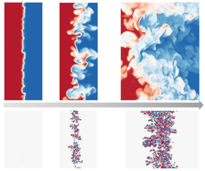
Unsteady mixing evolution typically progresses through three distinct stages: instability development, mixing transition and turbulent mixing. Taking the Rayleigh–Taylor (RT) mixing evolution as an example, for each stage figure 1 displays the corresponding density (upper) and vorticity (lower) fields, to reflect the characteristics of different stages.

Figure 1. Diagram of the three stages of RT mixing evolution. For each stage, the upper and lower images give the corresponding density and vorticity fields, respectively.
In the first stage, the amplitude of the perturbation remains small, featuring a negligible vorticity amplitude and a narrow mixing region. Thus the instability development during this stage is characterized as linear or weakly nonlinear, and analytical theoretical models have been proposed accordingly for single-mode perturbations (Layzer Reference Layzer1955; Mikaelian Reference Mikaelian1998; Goncharov Reference Goncharov2002; Liu, Zhang & Xiao Reference Liu, Zhang and Xiao2022; Zhang & Guo Reference Zhang and Guo2022; Liu et al. Reference Liu, Wu-Wang, Zhang and Xiao2023). Furthermore, for multi-mode cases, these analytical models are also applicable to depict the interfacial evolution, as the perturbed modes grow mostly independently (Rollin & Andrews Reference Rollin and Andrews2013; Canfield et al. Reference Canfield, Denissen, Francois, Gore, Rauenzahn, Reisner and Shkoller2020). In this stage, the linearly growing perturbations dominate the evolution, until the amplitude of the interfacial perturbation becomes comparable to the dominant wavelength.
As the flow progresses to the stage of mixing transition, the interfacial structures start to break into smaller scales, and multiscale behaviour appears due to the coupling and competition between different modes (Zhang & Ni Reference Zhang and Ni2023). Accordingly, the width of the mixing region and the perturbation amplitudes rapidly increase, leading to a pronounced shear effect and a significant increase in vorticity. Notably, for this stage, as shown in figure 1, the vorticity distribution exhibits remarkable inhomogeneity. High- and zero-vorticity regions distribute intermittently near the edges of the mixing region, as marked by the black box. In Richtmyer–Meshkov (RM) flows, where mixing rapidly develops under the impact of shock waves, the inhomogeneous vorticity distribution persists due to the influence of various complex waves, also suggesting the significance of the intermittency. Therefore, the mixing transition stage is characterized by strong nonlinearity, remarkable intermittency and local spatio-temporal dependency, which are intractable for existing analytical models. Attempting to track the development of multiple modes, the modal model has been proposed by Rollin & Andrews (Reference Rollin and Andrews2013) and Canfield et al. (Reference Canfield, Denissen, Francois, Gore, Rauenzahn, Reisner and Shkoller2020), combining Haan's mode coupling equations (Haan Reference Haan1991) and Goncharov's interface evolution model (Goncharov Reference Goncharov2002). Nevertheless, this method's applicability to the strongly nonlinear dynamics in the late mixing transition remains questionable, especially for multi-mode cases with complex mode interactions. Therefore, there is a pressing need to develop applicable methodologies for predicting the mixing transition.
Subsequently, the flow evolves into the turbulent mixing stage, corresponding to the well-mixed state of Dimotakis (Reference Dimotakis2000). In this stage, intense turbulent fluctuations further enhance the shear effect, resulting in a larger amplitude and distribution area of vorticity. Mixing at this stage displays self-similarity and deterministic statistical laws, making it suitable for RANS modelling (Dimonte & Tipton Reference Dimonte and Tipton2006; Kokkinakis et al. Reference Kokkinakis, Drikakis, Youngs and Williams2015; Kokkinakis, Drikakis & Youngs Reference Kokkinakis, Drikakis and Youngs2019; Zhang et al. Reference Zhang, He, Xie, Xiao and Tian2020; Xiao, Zhang & Tian Reference Xiao, Zhang and Tian2021; Xie, Zhao & Zhang Reference Xie, Zhao and Zhang2023).
It should be noted that the aforementioned three stages are not always discernible in practical applications. For RT flows, when the amplitudes of initial perturbations or the imposed acceleration are significant, mixing occurs rapidly, rendering the linear and transition stages negligible. Similarly, for RM flows, if the perturbation amplitudes or the incident shock wave Mach number are large, the first two stages can be difficult to observe. However, in many scenarios, the transition effect from a laminar to turbulent state is remarkable, and failing to capture the transition onset can cause significant deviations for numerical predictions. For instance, for the reshocked RM mixing flow where shock waves repeatedly impact the mixing region, Haines, Grinstein & Schwarzkopf (Reference Haines, Grinstein and Schwarzkopf2013) implemented a RANS experiment, where the turbulence model was switched on at different moments to model the effect of transition onset. Based on their observation, it is required to manually switch on the turbulence model at the reshocked moment, so that the RANS calculation can provide satisfactory results compared with implicit LES (ILES). This suggests that a model which is able to automatically detect the transition onset is desired for RANS prediction of mixing transition flows.
1.2. Challenges for RANS prediction of mixing transition flows
Although methodologies have been suggested for the stages of instability development and turbulent mixing, the intermediate mixing transition stage remains a formidable challenge for modelling endeavours due to the profoundly nonlinear behaviours of the perturbed modes. Existing RANS mixing models cannot be directly applied to the mixing transition stage due to their inherent limitation. Specifically, these models are grounded in the assumption of a homogeneous and fully developed turbulent mixing, which does not align with the characteristics of the transition stage. As evidenced by the high-fidelity (HiFi) numerical simulation analysis conducted by Livescu et al. (Reference Livescu, Ristorcelli, Gore, Dean, Cabot and Cook2009) and Morgan & Greenough (Reference Morgan and Greenough2015), the commonly used eddy viscosity closure and gradient diffusion approximation (GDA) within these existing RANS mixing models fall short in accurately describing the mixing transition. Furthermore, the distribution of the vorticity field depicted in figure 1 reveals a substantial intermittency during the transition stage, which has not been reflected by existing RANS models.
Despite the inherent difficulties for transition modelling, efforts have been made to improve the accuracy of RANS predictions for specific mixing transition flows. Firstly, artificially switching on the turbulence model when transition occurs is considered as one possible way to improve RANS results for mixing transition (Haines et al. Reference Haines, Grinstein and Schwarzkopf2013). However, this method deeply depends on the transition criteria. Various methods have been proposed to identify the transition onset. With observations for a series of steady flows, Dimotakis (Reference Dimotakis2000) proposed a transition threshold based on the outer-scale Reynolds number approximately at  $Re=1\sim 2\times 10^4$, which is derived from the emergence of an inertial range signifying the occurrence of transition. Zhou, Robey & Buckingham (Reference Zhou, Robey and Buckingham2003) extended Dimotakis's criterion to the unsteady mixing problem by introducing an additional temporal-associated length scale. Subsequently, Zhou (Reference Zhou2007) further extended the transient criterion of mixing transition and proposed a minimum turbulent state with
  $Re=1.6\times 10^5$, ensuring a sufficiently extended inertial range. It is noteworthy that the identification of the inertial range in these criteria can only be obtained based on a posteriori analysis of the energy spectrum, which cannot be used for real-time predictions. Recently, Wang et al. (Reference Wang, Song, Ma, Ma, Wang and Wang2022) proposed a transition criterion based on the mixing mass, enabling the identification of both the onset and cessation of transition. Nevertheless, global quantities like the mixing mass and the outer-scale Reynolds number fail to capture the local characteristics of transition, which are not compatible for practical RANS predictions.
Secondly, introducing other methods like the modal models or LES is helpful for describing the early-stage interfacial evolution, which can then provide information for initialization of RANS models, thereby achieving predictions for mixing transition. For example, for reshocked RM mixing, Kokkinakis, Drikakis & Youngs (Reference Kokkinakis, Drikakis and Youngs2020) implemented a ILES to depict the interfacial evolution prior to the shock passing, and the ILES results were used to give the initial turbulent kinetic energy for the turbulence model. Rollin & Andrews (Reference Rollin and Andrews2013) adopted the modal model to track the evolution of the perturbed modes, and subsequently applied the modal model's results to initialize the spatial profiles of the physical variables in RANS calculations. Moreover, Braun & Gore (Reference Braun and Gore2020) constructed a zero-dimensional passive model to provide initial conditions for a RANS model. In these combined schemes, however, there exists a common issue that the switching moment between RANS and the other method (the modal model or LES) needs to be clearly specified a priori.
To summarize, a feasible engineering prediction scheme for mixing transition flows is demanded, particularly in the context of RANS modelling studies. The objective of the present study is to develop a novel RANS mixing transition model, which is expected to have the following features. Firstly, it should be based on a uniform RANS framework for easy usage, and does not rely on other methods. Secondly, it should be able to autonomously predict the onset of transition and to accurately describe the spatio-temporal evolution of the transition process. Thirdly, it should be robust for different stages of various types of mixing flows, including typical RT/RM transition flows, and turbulent mixing flows that rapidly develop into a fully turbulent state with a negligible transition process. In order to address these, the key contribution of the proposed model is to accurately incorporate an intermittency model in RANS calculations of mixing transition flows. Inspired by boundary layer transition models (Menter et al. Reference Menter, Langtry, Likki, Suzen, Huang and Völker2006; Wang & Fu Reference Wang and Fu2011; Li, Ju & Zhang Reference Li, Ju and Zhang2023; Rosafio et al. Reference Rosafio, Lopes, Salvadori, Lavagnoli, Be and Misul2023), we introduce the intermittent factor  $\gamma$ and its transport equation, with
  $\gamma =0$ corresponding to a laminar state,
  $\gamma =1$ indicating a turbulent state and the intermediate values reflecting the transitional state. The present model will be extensively validated, showing its robustness in different cases.
The paper is organized as follows. We provide a comprehensive documentation of the modelling process in § 2. Specifically, § 2.1 outlines the governing equations and the baseline model, while § 2.2 details the key modelling idea about the intermittent factor  $\gamma$. Section 2.3 presents the validation of our strategy of introducing
  $\gamma$ to RANS calculations, and § 2.4 discusses the construction of the transport equation for
  $\gamma$. In § 3, we conduct systematic validations and tests for the proposed model. This section includes the validation of the
  $\gamma$ transport equation in § 3.1, sensitivity tests on model parameters in § 3.2 and an assessment of the accuracy and generalization performance of the present model in § 3.3. Finally, the key contributions of this study are summarized in § 4.
2. Methodology
2.1. Governing equations and baseline model
For interfacial mixing problems, the multicomponent RANS equations are solved by considering molecular transport and thermodynamic coefficients. The transport equations for the mean density  $\rho$, velocity
  $u_{i}$, total energy
  $E$ of the mixture and mass fraction
  $Y_{\alpha }$ of species
  $\alpha$ are given as follows:
 $$\begin{gather} \frac{\partial \bar{\rho }}{\partial t}+\frac{\partial \bar{\rho }{{{\tilde{u}}}_{j}}}{\partial {{x}_{j}}}=0, \end{gather}$$
 $$\begin{gather}\frac{\partial \bar{\rho }{{{\tilde{u}}}_{i}}}{\partial t}+\frac{\partial \bar{\rho }{{{\tilde{u}}}_{i}}{{{\tilde{u}}}_{j}}}{\partial {{x}_{j}}}+\frac{\partial \bar{p}}{\partial {{x}_{i}}}-\bar{\rho}g_{i}={-}\frac{\partial \tau_{ij}}{\partial {{x}_{j}}}+\frac{\partial {{{\bar{\sigma}}}_{ij}}}{\partial {{x}_{j}}}, \end{gather}$$
 $$\begin{gather}\frac{\partial \bar{\rho }\tilde{E}}{\partial t}+\frac{\partial (\bar{\rho }\tilde{E}+\bar{p}){{{\tilde{u}}}_{j}}}{\partial {{x}_{j}}}-\bar{\rho}\tilde{u}_{i}g_{i}=D_{E}+D_{K}+\frac{\partial }{\partial {{x}_{j}}}(-{\tau}_{ij}{{\tilde{u}}_{i}}+{{\bar{\sigma }}_{ij}}{{\tilde{u}}_{i}} -\bar{q}_{c}-\bar{q}_{d}), \end{gather}$$
 $$\begin{gather}\frac{\partial \bar{\rho }{{{\tilde{Y}_{\alpha}}}}}{\partial t}+\frac{\partial \bar{\rho }{{{\tilde{Y}_{\alpha}}}}{{{\tilde{u}}}_{j}}}{\partial {{x}_{j}}}=D_{Y}+\frac{\partial }{\partial {{x}_{j}}}\left(\bar{\rho}\bar{D}\frac{\partial\tilde{Y}_{\alpha}}{\partial x_{j}}\right). \end{gather}$$
The overbar and tilde represent the Reynolds- and Favre-averaged fields, respectively. Moreover, subscripts  $i,j=1,2,3$ denote the three spatial directions (
 $x,y,z$), and
  $t$ denotes time. Furthermore, the heat flux
  $\bar {q}_{c}$, the interspecies diffusional heat flux
  $\bar {q}_{d}$, and the viscous stress tensor
  $\bar {\sigma }_{ij}$ are given as
 $$\begin{gather} \bar{q}_{c}={-}\bar{\kappa} \partial \tilde{T}/\partial x_{j}, \end{gather}$$
 $$\begin{gather}\bar{q}_{d}={-}\sum \bar{\rho} \bar{D}C_{p,\alpha}\tilde{T}\partial \tilde{Y}_{\alpha}/\partial x_{j}, \end{gather}$$
 $$\begin{gather}\bar{\sigma}_{ij}= 2\bar{\mu}(\tilde{S}_{ij}-\tilde{S}_{kk}\delta_{ij}/3), \quad \tilde{S}_{ij}=(\partial \tilde{u}_{i}/\partial x_{j}+\partial \tilde{u}_{j}/\partial x_{i})/2. \end{gather}$$
Here,  $\bar {\mu }$,
  $\bar {D}$,
  $\bar {\kappa }$,
  $C_{p,\alpha }$ and
  $g_{i}$ represent dynamic viscosity, mass diffusivity, thermal conductivity, constant-pressure specific heat of species
  $\alpha$ and gravitational acceleration in the
  $i$ direction, respectively. In addition, the equation of state (EOS)
  $\bar {p}M=\bar {\rho }R\tilde {T}$ for the perfect gas is used, with
  $M$ and
  $R$ denoting the molar mass and the gas constant, respectively. Note that the EOS for the mixture is calculated under the assumptions of iso-temperature (i.e.
  $T_1=T_2=\cdots =T_{\alpha }$) and partial pressure (i.e.
  $p=\sum {p}_{\alpha }$) and the fluid properties of the mixture are determined using a species-linearly weighted assumption (Livescu Reference Livescu2013).
Equations (2.1)–(2.4) are deduced based on the concept of ensemble averaging, which results in the unclosed terms including the Reynolds stress  $\tau _{ij}$, the turbulent diffusion of the total energy
  $D_{E}=-\partial (\bar {\rho }\widetilde {{u}_{j}''e''}+\overline {pu_{j}''})/\partial x_{j}$, the turbulent diffusion of the turbulent kinetic energy (TKE,
  $\tilde {K}$)
  $D_{K}=-\partial (\bar {\rho }\widetilde {{u}_{i}''{u}_{i}''{u}_{j}''}/2)/\partial x_{j}$ and the turbulent diffusion of the mass fraction
  $D_{Y}=-\partial (\bar {\rho }\widetilde {u_{j}''{Y_{\alpha }}''})/\partial x_{j}$, respectively, the double prime here denoting Favre fluctuation. In previous studies, numerous turbulent mixing models have been proposed to model these unclosed terms, which mostly focus on fully developed turbulence. Taking the well-developed K-L model as an example, the turbulent transport terms are modelled by the GDA
 \begin{equation} -\bar{\rho}\widetilde{u_{j}''f''}=\frac{\mu_{t}}{N_{f}}\frac{\partial \tilde{f}}{\partial x_{j}}, \end{equation}
where  $f$ denotes an arbitrary physical variable and
  $N_{f}$ is the corresponding model coefficient. Thus, the turbulent diffusion terms are respectively modelled as
 $$\begin{gather} {D}_{E}=\frac{\partial}{\partial x_{j}}\left(\frac{\mu_{t}}{N_{h}}\frac{\partial \tilde{h}}{\partial x_{j}}\right ), \end{gather}$$
 $$\begin{gather}{D}_{K}=\frac{\partial}{\partial x_{j}}\left(\frac{\mu_{t}}{N_{K}}\frac{\partial \tilde{K}}{\partial x_{j}}\right ), \end{gather}$$
 $$\begin{gather}{D}_{Y}= \frac{\partial}{\partial x_{j}}\left(\frac{\mu_{t}}{N_{Y}}\frac{\partial \tilde{Y}}{\partial x_{j}}\right), \end{gather}$$
where  $h$ represents enthalpy. Importantly, the turbulent viscosity
  $\mu _{t}$ is described by the TKE
  $\tilde {K}$ and the turbulent length scale
  $\tilde {L}$
 \begin{equation} \mu_{t}=C_{\mu}\bar{\rho} \tilde{L}\sqrt{2\tilde{K}}, \end{equation}
where  $C_{\mu }$ is a model coefficient. With the classical Boussinesq eddy viscosity hypothesis, the Reynolds stress is modelled as
 \begin{equation} {{{\tau }}_{ij}}={{C}_{P}}\bar{\rho }\tilde{K}{{\delta }_{ij}}-2{{\mu }_{t}}(\tilde{S}_{ij}-\tilde{S}_{kk}{{\delta }_{ij}}/3), \end{equation}
where  $C_{P}$ is a model coefficient.
Additionally, the transport equations of the TKE and  $\tilde {L}$ are
 $$\begin{gather} \frac{\partial \bar{\rho }\tilde{K}}{\partial t}+\frac{\partial \bar{\rho }{{{\tilde{u}}}_{j}}\tilde{K}}{\partial {{x}_{j}}}={-}{{{\tau }}_{ij}}\frac{\partial {{{\tilde{u}}}_{i}}}{\partial {{x}_{j}}}+\frac{\partial }{\partial {{x}_{j}}}\left(\frac{{{\mu }_{t}}}{{{N}_{K}}}\frac{\partial \tilde{K}}{\partial {{x}_{j}}}\right)+{{S}_{Kf}}-D_{r}, \end{gather}$$
 $$\begin{gather}\frac{\partial \bar{\rho }\tilde{L}}{\partial t}+\frac{\partial \bar{\rho }{{{\tilde{u}}}_{j}}\tilde{L}}{\partial {{x}_{j}}}=\frac{\partial }{\partial {{x}_{j}}}\left(\frac{{{\mu }_{t}}}{{{N}_{L}}}\frac{\partial \tilde{L}}{\partial {{x}_{j}}}\right)+{{C}_{L}}\bar{\rho }\sqrt{2\tilde{K}}+{{C}_{C}}\bar{\rho }\tilde{L}\frac{\partial {{{\tilde{u}}}_{j}}}{\partial {{x}_{j}}}. \end{gather}$$
Here, the right-hand side terms of (2.14) represent the shear production, turbulent diffusion, buoyancy production  ${{S}_{Kf}}$ and drag
  $D_{r}={{C}_{D}}\bar {\rho }{{( \sqrt {2\tilde {K}})}^{3}}/{\tilde {L}}$, respectively. The right-hand side terms of (2.15) include the turbulent diffusion, production and compression, successively. In particular, the buoyancy production term
  ${{S}_{Kf}}$ is given based on the formation proposed by Kokkinakis et al. (Reference Kokkinakis, Drikakis, Youngs and Williams2015) as
 \begin{equation} {{S}_{Kf}}=C_{B}\bar{\rho}\sqrt{2\tilde{K}}A_{L}g_{i}, \quad A_{L}=C_{A}\tilde{L}(\partial \bar{\rho}/\partial x_{i})/\bar{\rho}. \end{equation}
More details about the K-L model can be found in Zhang et al. (Reference Zhang, He, Xie, Xiao and Tian2020).
The K-L model presented in this section is used as the baseline model hereafter, and the baseline-standard model coefficients following Zhang et al. (Reference Zhang, He, Xie, Xiao and Tian2020) are listed in table 1. Developed for fully developed turbulence, the baseline K-L model is not suitable for the mixing transition stage. The next section will introduce the general idea of constructing the mixing transition model based on the baseline model.
Table 1. The baseline-standard model coefficients of the K-L model.

2.2. Introducing the intermittent factor to the mixing transition model
In the transition process, the mixing flow undergoes dramatic variations from laminar to turbulent states, exhibiting significant intermittency and local spatio-temporal dependence. Specifically, turbulent and non-turbulent regions are intermittently distributed in the mixing region shown in figure 1. This intermittent nature of transition has not been considered in existing RANS mixing models, and this might cause unsatisfactory results. Inspired by boundary layer transition modelling in aerospace engineering, we introduce the intermittent factor  $\gamma$ to mixing flows in the present study, in order to capture the intermittent characteristics in RANS mixing transition models.
For transitional flows, the concept of the intermittent factor is usually considered as the possibility of the local flow being turbulent or not. The quantification of  $\gamma$, however, can be non-trivial, particularly due to the difficulty of distinguishing turbulent and non-turbulent regions in unsteady mixing flows. Similar to the definition applied in free jets (Gauding et al. Reference Gauding, Bode, Brahami, Varea and Danaila2021), we use the enstrophy
  $\omega ^2$ for the quantification of
  $\gamma$ in the present study. Firstly, an indicator function is specified as
 \begin{equation} I(x_i,t)\equiv F(\omega^2(x_i,t)-\omega^2_0), \end{equation}
where  $F$ is the Heaviside function. Moreover,
  $\omega ^2_0$ is a threshold value that is widely accepted in free shear flows to define the interface of turbulent and non-turbulent regions (Holzner et al. Reference Holzner, Liberzon, Nikitin, Luthi, Kinzelbach and Tsinober2008; da Silva et al. Reference da Silva, Hunt, Eames and Westerweel2014; Silva, Zecchetto & Da Silva Reference Silva, Zecchetto and Da Silva2018; Watanabe, Da Silva & Nagata Reference Watanabe, Da Silva and Nagata2019), and the value of
  $\omega ^2_0$ can be obtained from the probability density function (PDF) of the enstrophy distribution (see Gauding et al. Reference Gauding, Bode, Brahami, Varea and Danaila2021). Determination of the
  $\omega ^2_0$ mainly includes 3 steps, which are introduced briefly as follows and the detailed contents will be published elsewhere. Firstly, plot the PDF of enstrophy distribution. Specially, the local enstrophy is normalized by
  $\hat {\omega }$,
 \begin{equation} \hat{\omega}=\frac{\displaystyle\int\langle \omega^2\rangle^2\, {{\rm d}\kern0.07em x}}{\displaystyle\int\langle\omega^2\rangle\, {\rm d}\kern0.07em x}, \end{equation}
here,  $\langle \rangle$ represents averaging in the homogeneous
  $y$–
$y$– $z$ plane perpendicular to the mixing development direction
  $x$. The PDF of the enstrophy distribution exhibits two peaks, one representing the non-turbulent region, and the other representing the turbulent region. Secondly, find a possible enstrophy value to define the interface separating the non-turbulent and turbulent regions. Thirdly, determine the threshold by calculating the structure function for two points in space. By repeating the abovementioned steps at different moments, we can get the corresponding enstrophy threshold, which is different for different moments.
Thereafter, the intermittent factor  $\gamma (x,t)$ is obtained by
 \begin{equation} \gamma(x,t)=\langle I(x_i,t)\rangle. \end{equation}
Note that the definition here indicates that  $\gamma$ varies from
  $0$ to
  $1$. Moreover, based on the analysis for the HiFi
  $\gamma$ profiles, it is noted that the spatial profiles of the late-time intermittent factor collapse together, exhibiting a self-similar characteristic.
With the intermittent factor  $\gamma$, we now reformulate the turbulence models used for RANS calculation of mixing flows. In particular, the turbulent viscosity in the Reynolds stress closure is the key term to be considered here. Given that the widely used baseline closure in (2.12) is designed for fully developed turbulence, violating the real physics of the transition process, the turbulent viscosity closure requires further modification to capture the intermittent nature of the transition process. Therefore, introducing the intermittent factor
  $\gamma$, the turbulent viscosity
  $\mu _{t}$ is replaced with an effective eddy viscosity
  $\mu _{eff}$, which is written as
 \begin{equation} \mu_{eff}=(1-\gamma)\mu_{nt}+\mu_{new}, \quad \mu_{new}=\gamma\mu_{t}. \end{equation}
Here,  $\mu _{nt}$ (‘nt’ means non-turbulent) involves a complex influence of different instability modes. For example, in boundary layer transition modelling (Wang & Fu Reference Wang and Fu2011),
  $\mu _{nt}$ involves the information of the first and second modes, cross-flow mode and so on. However, for interfacial mixing flows, the existing studies do not cover this aspect, thus
  $\mu _{nt}$ is left for future study. Consequently,
  $\tau _{ij}$ can be reformulated as
 \begin{equation} \tau_{ij}={{C}_{P}}\bar{\rho }\tilde{K}{{\delta }_{ij}}-2{{\mu }_{new}}(\tilde{S}_{ij}-\tilde{S}_{kk}{{\delta }_{ij}}/3), \quad \mu_{new}=\gamma\mu_{t}=C_{\mu}\gamma\bar{\rho}\tilde{L}\sqrt{2\tilde{K}}. \end{equation}
Accordingly, in the turbulent diffusion term modelled by the GDA,  $\mu _{t}$ is also replaced by
  $\mu _{new}$ in the new transition model.
Equation (2.21) indicates that, when  $\gamma$ is very small, the model provides a negligible Reynolds stress, indicating a non-turbulent state. As
  $\gamma$ gradually increases,
  $\mu _{new}$ grows and ultimately recovers to the original
  $\mu _t$ when
  $\gamma =1$, correspondingly, the closure of the Reynolds stress back to (2.13). Particularly,
  $\gamma$ is expected to quantify the intermittency, providing a reasonable way to model the growth of turbulent fluctuations in the mixing transition stage.
2.3. Validation of introducing intermittent factor to RANS prediction
In order to validate the strategy of introducing  $\gamma$ to RANS modelling, a three-dimensional (3-D) HiFi simulation of RT mixing with the Atwood number
  $A_t=(\rho _1-\rho _2)/(\rho _1+\rho _2)=0.5$,
  $\rho _1$ and
  $\rho _2$ representing the densities of the heavy and light fluids respectively, has been performed to extract the distributions of the intermittent factor
  $\gamma$. Subsequently, the
  $\gamma _{HiFi}$ extracted from the HiFi simulation is directly incorporated into the new formulation in (2.21) to conduct a RANS calculation. With this numerical experiment, we attempt to answer the following question. Given accurate quantification of
  $\gamma$, is the new formulation in (2.21) able to predict the transition process in RANS calculations?
In the 3-D HiFi simulation, the mass fraction  $\tilde {Y}$ is initialized to follow an error function profile in the
  $x$ direction, i.e.
 \begin{equation} \tilde{Y}=0.5\left[1+\tanh\left(\frac{x- \xi(y,z)}{H_{0}}\right)\right], \end{equation}
where  $\xi (y,z)$ represents the random perturbation imposed at the initial interface, and
  $H_0=0.0008$ cm is the pseudo-interface thickness. The profile (2.22) results in an initial diffusive mixing layer lying across 4 grid points with the width of
  $0.025$ cm, which characterizes the initial perturbation amplitude and is reflected by setting the initial value of the turbulent length scale
  $\tilde {L}_0$ in RANS calculation, as listed in table 2. More details about the configuration of the HiFi simulation are documented in Appendix A.
Table 2. List of the calculated cases. The ‘perturbation type’ represents whether the initial perturbations of the experiments and 3-D simulations corresponding to these cases only include short waves or also include long waves.

With the aid of  $\gamma _{HiFi}$, we implement the corresponding 1-D RANS calculation for this 3-D case. The baseline-standard model coefficients listed in table 1 are used here. We focus on the temporal evolution of total mixing width, which is considered as the most important statistical quantity for engineering applications, and is calculated based on the straightforward species-truncated definition, i.e.
 \begin{equation} H\equiv x|_{\psi=0.99}-x|_{\psi=0.01}, \end{equation}
where  $x|_{\psi =0.99}$ and
  $x|_{\psi =0.01}$ represent the locations of the heavy fluid with Favre-averaged volume fractions of 0.99 and 0.01. Figure 2 indicates that the baseline model consistently overpredicts the evolution of the mixing width, exhibiting a quadratic curve throughout its progression. By contrast, due to the introduction of the intermittent factor
  $\gamma _{HiFi}$, the predictive accuracy is significantly improved. In particular, the instability and transition stages of mixing evolution are well described, aligning with HiFi results. This numerical experiment provides a clear evidence that the strategy of introducing
  $\gamma$ as in (2.21) is effective for RANS calculations of mixing transition flows.

Figure 2. Predictions for temporal evolution of the truncated mixing width for the HiFi RT simulation.
2.4. Transport equation of the intermittent factor for mixing flows
In practical RANS calculations, we usually do not have precursor HiFi data for the  $\gamma$ distribution. Therefore, in order to consider the effect of intermittency in RANS, it is necessary to build a model for depicting the spatio-temporal evolution of the intermittent factor. In this section, a transport equation for
  $\gamma$ is constructed.
Following the framework of constructing the boundary layer transition models based on the intermittent factor (Menter, Esch & Kubacki Reference Menter, Esch and Kubacki2002; Wang & Fu Reference Wang and Fu2011), we present the  $\gamma$ transport equation as follows:
 \begin{equation} \frac{\partial \bar{\rho }\gamma}{\partial t}+\frac{\partial \bar{\rho }{{{\tilde{u}}}_{j}}\gamma}{\partial {{x}_{j}}}=\frac{\partial }{\partial {{x}_{j}}}\left[\left(\bar{\mu}+\frac{{{\mu }_{new}}}{{{N}_{\gamma}}}\right)\frac{\partial \gamma}{\partial {{x}_{j}}}\right]+P_{\gamma}-\epsilon_{\gamma}, \end{equation}
where  $P_{\gamma }$ and
  $\epsilon _{\gamma }$ represent the product and dissipation terms, respectively, and
  $N_{\gamma }$ is a model coefficient. As the mixing flow eventually evolves to a fully developed turbulent state, the new formulation (2.21) should ultimately approach the original formation (2.13). Correspondingly,
  $\gamma$ should grow to 1 and subsequently fluctuate around 1 due to the fluctuating nature of turbulence. Accordingly, we introduce
  $\epsilon _{\gamma }=\gamma P_{\gamma }$, which ensures that
  $P_{\gamma }-\epsilon _{\gamma }$ provides a positive net increment during transition, and then tends to
  $0$ for the fully developed turbulence.
The production of the intermittent factor  $P_{\gamma }$ is thus the key term to be closed for the transition model, which is expected to feature two functions, i.e. identifying the onset of transition and depicting the evolution of
  $\gamma$ during the transitional process. It is formulated as
 \begin{equation} P_{\gamma}=F_{onset}G_{r}, \end{equation}
where  $F_{onset}$ serves as a transition switch, and
  $G_{r}$ describes the growth of
  $\gamma$.
Here,  $F_{onset}$ is expressed as
 \begin{equation} F_{onset}=1-\frac{1}{{\rm e}^{max(0,Re_{t}-Re_{tra})}}, \quad Re_{t}=\frac{\tilde{L}\sqrt{\tilde{K}}}{\nu}, \end{equation}
where  $\nu$ represents the molecular kinematic viscosity of the mixture,
  $Re_{t}$ is the local turbulent Reynolds number and
  $Re_{tra}$ is a pre-defined key transition threshold value. Based on the formulation proposed here,
  $F_{onset}$ is expected to have the following features. Firstly,
  $Re_{t}$ is calculated using
  $\tilde {K}$ and
  $\tilde {L}$ obtained from the corresponding transport equations (2.14) and (2.15), which characterize the spatial-temporal distribution of the local turbulent state. It is noted that the distribution of
  $Re_{t}$ is obviously affected by the initial conditions for the turbulence models in RANS calculations, so that
  $F_{onset}$ here can reflect the sensitivity of the transition models to initial perturbations. Secondly, the transition model is activated when
  $Re_{t}>Re_{tra}$, with the threshold value
  $Re_{tra}=10$ set based on the DNS data from Livescu, Wei & Brady (Reference Livescu, Wei and Brady2021). Thirdly, with the
  $exp$ function, the local value of
  $F_{onset}$ rapidly grows to
  $1$ once transition occurs.
The function  $G _{r}$ dominates the evolution of the intermittent factor
  $\gamma$, and is given as
 \begin{align}
G_{r}&=C_{1}\sqrt{\gamma}\left\{ \underbrace{ (1-\gamma)
\left[\bar{\rho}\sqrt{2\tilde{S}_{ij}\tilde{S}_{ij}}+C_{2}\sqrt{\max
\left(0,-\frac{\partial \bar{\rho}}{\partial x_k}
\frac{\partial \bar{p}}{\partial
x_k}\right)}\right]}_{\mathit{mean\ field}}\right.\nonumber\\
&\quad +\left.\underbrace{
\left(\gamma S_{Kf}-{{{\tau }}_{ij}}\frac{\partial
{{{\tilde{u}}}_{i}}}{\partial
{{x}_{j}}}\right)/\tilde{K}}_{\mathit{turbulent\
fluctuating\ field}} \right\},
\end{align}
\begin{align}
G_{r}&=C_{1}\sqrt{\gamma}\left\{ \underbrace{ (1-\gamma)
\left[\bar{\rho}\sqrt{2\tilde{S}_{ij}\tilde{S}_{ij}}+C_{2}\sqrt{\max
\left(0,-\frac{\partial \bar{\rho}}{\partial x_k}
\frac{\partial \bar{p}}{\partial
x_k}\right)}\right]}_{\mathit{mean\ field}}\right.\nonumber\\
&\quad +\left.\underbrace{
\left(\gamma S_{Kf}-{{{\tau }}_{ij}}\frac{\partial
{{{\tilde{u}}}_{i}}}{\partial
{{x}_{j}}}\right)/\tilde{K}}_{\mathit{turbulent\
fluctuating\ field}} \right\},
\end{align}
where  $C_{1}$ and
  $C_{2}$ are model coefficients. The function
  $G_r$ superimposes the mean field and the turbulent fluctuating field, both of which consist of buoyancy and shear effects. They synergistically decide the spatio-temporal evolution of the intermittent factor
  $\gamma$. Specifically, the mean field includes the amplitude of the mean shear strain rate and the baroclinic term that represents the mean buoyancy effect, which is then multiplied by
  $(1-\gamma )$ according to the definition of the intermittency, while the turbulent fluctuating field includes the turbulent shear and buoyancy terms. It is noted that the baroclinic term promotes the development of instability when it is negative; otherwise, it does not contribute to the flow evolution. Therefore, the form
  $\max (0,-({\partial \bar {\rho }}/{\partial x_k}) ({\partial \bar {p}}/{\partial x_k}))$ is used here, and the square root is used to ensure dimensional consistency. For the mean field, the mean buoyancy term is multiplied by
  $C_2$, which is used to adjust the weight between the mean shear and mean buoyancy effects during the mixing transition process. Note that for the interfacial mixing problems considered here, the KH effect represented by the mean shear dominates the transition, hence
  $C_2$ is set to a small value (
 $C_2=0.015$) to ensure this. Furthermore, since the closure for the turbulent buoyancy production term
  $S_{Kf}$ is designed for the fully developed turbulent state, it is multiplied by
  $\gamma$ to ensure a reasonable description for the mixing transition process. Note that the Reynolds stress
  $\tau _{ij}$ has included the intermittent factor because of the closure (2.21). The variable
  $\tilde {K}$ in the denominator ensures dimensional consistency. In addition, based on the analysis for HiFi simulation of RT mixing transition flow, it is also noted that, once transition occurs,
  $\gamma$ will rapidly increase to 1 with a steep growth rate, which is achieved by introducing the overall coefficient
  $C_1\sqrt {\gamma }$.
The main mechanism dominating the  $\gamma$ evolution is different at different stages during the mixing evolution process, which is verified in figure 3. Here, we plot the temporal evolution of the ratio between the mean field and the sum of the two fields integrated along the
  $x$ direction, i.e. the mixing development direction. Figure 3 indicates that the mean flow dominates the early-time evolution and triggers the transition onset. When the fluctuating field gradually becomes prominent, the turbulent flow dominates the
  $\gamma$ evolution.

Figure 3. Temporal evolution of the ratio between the mean field and the sum of the two fields integrated along the mixing development direction  $x$.
$x$.
To conclude, each part of the product term  $P_{\gamma }$ has its specific function, and it is expected that, under their synergy, mixing transition flows can be accurately predicted.
3. Model validation
3.1. Validation of the transport equation for the intermittent factor
To validate whether the proposed  $\gamma$ transport equation (2.24) can accurately describe the spatio-temporal evolution of the intermittent factor, we perform a RANS calculation for the HiFi case, based on the (2.24).
Here, the used model coefficients are different from the baseline-standard values listed in table 1. The reason is explained as follows. The baseline-standard values are from Zhang et al. (Reference Zhang, He, Xie, Xiao and Tian2020), which proposes a methodology to theoretically derive the constraint relations among the model coefficients of the K-L model. By inputting several known variables into those relations, such as  $\alpha _b$ (the bubble growth rate in RT mixing),
  $\theta _b$ (the power exponent of bubble growth in RM mixing),
  $\alpha _{KH}$ (the growth rate of KH mixing) and so on, the specific model coefficient values can be obtained immediately. Moreover, once we substitute the obtained model coefficients into RANS equations to calculate RT/RM/KH mixing problems, RANS predictions can give the corresponding self-similar growth rate.
For RT mixing flows,  $\alpha _b$ is the key parameter to decide the late-time self-similar scaling. However, the value of
  $\alpha _b$ is not a universal constant and sensitively depends on the initial perturbations. Reliable numerical simulations (Youngs Reference Youngs2013) indicate that
  $\alpha _b$ varies in the range of
  $0.025\sim 0.12$ when different initial perturbations are adopted, particularly
  $\alpha _b \sim 0.025$ if the initial perturbations have only short waves (Cabot & Cook Reference Cabot and Cook2006; Livescu et al. Reference Livescu, Wei and Brady2021), with
  $\alpha _b$ exhibiting a relatively larger value if the initial perturbations include long waves. In addition,
  $\alpha _b$ is approximatively 0.05 for natural perturbations, as the linear electric motor (LEM) experiment.
However, it is fairly well known that the ability of RANS models to characterize initial perturbations is quite limited and they cannot really capture the differences between initial perturbations’ modes. To enable RANS predictions to reproduce those different self-similar growth rates, the methodology proposed in Zhang et al. (Reference Zhang, He, Xie, Xiao and Tian2020) implicitly considers the influence of initial perturbations and inserts the self-similar growth rates into the determination process of the model coefficients, so that the obtained model coefficients can reproduce the corresponding self-similar scaling.
In Zhang et al. (Reference Zhang, He, Xie, Xiao and Tian2020), the targeted flow is the LEM experiment, thus the model coefficients, i.e. the values listed in table 1, are set to produce  $\alpha _b \sim 0.05$. However, for the present HiFi RT case, the late-time quadratic growth rate
  $\alpha _b$ is approximately 0.04 by the formula
  $\alpha _b=(dh_b/dt)^2/(4A_tgh_b)$,
  $h_b$ representing the bubble width. Therefore, for the present case we set the corresponding model coefficients listed in ‘long wave’ of table 3 to reproduce
  $\alpha _b\sim 0.04$. Moreover, the baseline model also uses the same coefficients to produce the same late-time growth rate.
Table 3. The used model coefficients of the present model for all the calculated cases. Here, the ‘short (long) wave’ represents the perturbation type of the cases listed in table 2. The baseline and the present models adopt the same model coefficients.

The initial values of the turbulence model variables are set as follows. The initial  $\tilde {L}_0$ is set to match the initial mixing layer width in the 3-D HiFi simulations, while the initial TKE
  $\tilde {K}_0$, which does not have a physical determination method, is given a small value to ensure a correct implementation of the RANS simulation (Dimonte & Tipton Reference Dimonte and Tipton2006; Morán-López & Schilling Reference Morán-López and Schilling2013; Denissen et al. Reference Denissen, Rollin, Reisner and Andrews2014; Kokkinakis et al. Reference Kokkinakis, Drikakis and Youngs2019; Xiao, Zhang & Tian Reference Xiao, Zhang and Tian2020; Zhang et al. Reference Zhang, He, Xie, Xiao and Tian2020). The initial intermittent factor
  $\gamma _0$ is set to a small value of
  $1\times 10^{-16}$ near the interface to enable the successful activation of the RANS model, while in other regions
  $\gamma _0$ is set to 0.
Figure 4 shows the temporal evolution of the truncated mixing width  $H$. The good agreement between the present model and the HiFi results demonstrates that the introduction of the
  $\gamma$ transport equation (2.24) can effectively improve the RANS predictions for this mixing transition. In addition, it is clear that the baseline model and the present transition model give the same growth rate as the flow evolves to turbulence, because they use the same model coefficients to achieve the same late-time self-similar rate. However, due to the fact that the baseline model is constructed under the assumption of fully developed turbulence, it always gives a quadratic evolution, even for the instability and transition stages. In the inset the temporal evolution of the maximum value
  $\gamma _{max}$ of the intermittent factor is shown and reasonably agrees with the HiFi results. This suggests that the
  $\gamma$ transport equation is able to capture the evolution of the intermittent factor in this case. Specifically,
  $\gamma _{max}$ remains zero in the initial stage of mixing evolution, implying a poorly mixed and non-turbulent state before approximately
  $t=1.3$ s, and then exhibits a remarkable inflection point at
  $t=1.3$ s, signifying the onset of transition. Thereafter,
  $\gamma _{max}$ rapidly approaches
  $1$. These variations agree well with our expectations to a mixing transition model. Moreover, figure 4 shows that the sudden increases of
  $H$ and
  $\gamma _{max}$ both occur at approximately
  $t=1.3$ s, suggesting that the
  $\gamma$ transport equation (2.24) has been closely coupled with the underlying model, successfully triggering the transition onset.

Figure 4. Prediction for temporal evolutions of the truncated mixing width  $H$, and the maximum value
  $\gamma _{max}$ of the intermittent factor (inset).
In addition to the temporal evolution, the spatial profiles of the intermittent factor scaled by its maximum value are shown in figure 5. Overall, the  $\gamma$ profiles predicted by the present transition model agree well with the HiFi results. This further indicates that the transport equation (2.24) is constructed reasonably and models the
  $\gamma$ evolution well.

Figure 5. Spatial profiles of the intermittent factor scaled by its maximum value. (a–d) Correspond to  $t=1.63$ s,
  $t=2.65$ s,
  $t=3.63$ s and
  $t=4.56$ s, respectively.
3.2. Sensitivity tests on model parameters
The present model additionally introduces 4 model coefficients, i.e.  $N_\gamma$ in the diffusion term,
  $C_1$ and
  $C_2$ in the production term (2.27) and the transition threshold
  $Re_{tra}$ in the transition switch function (2.26). The sensitivity of these coefficients is tested in this part. In addition, the influence of the initial
  $\tilde {L}_0$ and
  $\tilde {K}_0$ on the prediction results of the present model is also verified.
3.2.1. Sensitivity tests on the model coefficients
Firstly, the sensitivity of  $N_\gamma$ is checked. In general, the diffusion coefficient influences the shape of the spatial profile, thus the
  $\gamma$ profiles at
  $t=7$ s in figure 6(a) with different
  $N_\gamma$ are displayed. This indicates that
  $N_\gamma$ indeed influences the intermittent factor's diffusion behaviour such that a smaller
  $N_\gamma$ leads to a more diffused spatial distribution, which is attributed to the fact that a smaller
  $N_\gamma$ results in a larger diffusion term.

Figure 6. (a) Spatial profiles of the scaled intermittent factor with different  $N_\gamma$; (b) temporal evolutions of
  $\gamma _{max}$ and the total mixing width with different
  $Re_{tra}$; (c) temporal evolutions of
  $\gamma _{max}$ and the total mixing width with different
  $C_{1}$; (d) temporal evolutions of
  $\gamma _{max}$ and the total mixing width with different
  $C_2$; (e) temporal evolutions of
  $\gamma _{max}$ and the total mixing width with different
  $\tilde {K}_0$; ( f) temporal evolutions of
  $\gamma _{max}$ and the total mixing width with different
  $\tilde {L}_0$.
The sensitivity test on  $Re_{tra}$ is shown in figure 6(b), where the temporal evolutions of the maximum values of the intermittent factor and the total mixing width are plotted, indicating that
  $Re_{tra}$ mainly impacts the transition onset, a larger
  $Re_{tra}$ causing a later transition.
Next, we test the sensitivity of  $C_1$ and
  $C_2$. Figure 6(c,d) gives the temporal evolutions of the maximum values of the intermittent factor and the total mixing width with different
  $C_2$ and
  $C_1$. It indicates that
  $C_2$ significantly affects the transition moment, and a larger
  $C_2$ results in an earlier transition. This is attributed to the fact that a larger
  $C_2$ results in a larger mean buoyancy term, corresponding to a stronger force to trigger the transition. The parameter
  $C_1$ directly changes the amplitude of the production term of the
  $\gamma$ transport equation, thus a larger value results in a larger growth rate of the intermittent factor.
In the present study, the values of  $N_\gamma$,
  $C_1$ and
  $C_2$ are calibrated based on the HiFi RT case, while
  $Re_{tra}=10$ is determined based on the DNS data of Livescu et al. (Reference Livescu, Wei and Brady2021). These values are consistently used for all the cases in the present study.
3.2.2. Sensitivity tests on the initial  $\tilde {L}_0$ and $\tilde {K}_0$


For practical applications, achieving an accurate control for the transition onset is crucial, which has been considered in (2.26) of the  $F_{onset}$. Specifically, the influence of the initial conditions
  $\tilde {L}_0$ and
  $\tilde {K}_0$ on the transition onset are tested by two sets of RANS calculations. The first group maintains a fixed
  $\tilde {L}_0=0.025$ cm to match the initial mixing layer width in the HiFi simulation while varying
  $\tilde {K}_0$ from
  $2.5\times 10^{-8}$ to
  $2.5\times 10^{-2}\ {\rm cm}^2\ {\rm s}^{-2}$. The second group keeps a fixed
  $\tilde {K}_0=2.5\times 10^{-6}\ {\rm cm}^2\ {\rm s}^{-2}$ and changes
  $\tilde {L}_0$ from 0.01 to 0.05 cm. Figure 6(e, f) gives the temporal evolution of
  $\gamma _{max}$ and the mixing width
  $H$ for different initial conditions, revealing that both
  $\tilde {L}_0$ and
  $\tilde {K}_0$ indeed affect the onset of transition, and larger initial values lead to an earlier transition (Youngs Reference Youngs2013; Ni, Zeng & Zhang Reference Ni, Zeng and Zhang2023).
However, note that the present model is more sensitive to variation of  $\tilde {L}_0$, as a slight increment can significantly promote the transition. In comparison,
  $\tilde {K}_0$ differs by several orders of magnitude in these tests, while the deviation in figure 6(e) is not significant. Moreover, comparing the sensitivity of
  $Re_{tra}$ with that of the initial
  $\tilde {L}_0$ and
  $\tilde {K}_0$, we can see that influence of the
  $Re_{tra}$ is much weaker than
  $\tilde {L}_0$ and stronger than
  $\tilde {K}_0$. This is attributed to the fact that
  $Re_{tra}$ only affects the model's judgement for the local transition behaviour, while
  $\tilde {L}_0$ is closely related to the initial perturbation amplitude and significantly influences the evolutionary velocity of mixing flows. A larger
  $\tilde {L}_{0}$ signifies a more significant initial perturbation, thereby promoting the mixing evolution. The insensitivity of the present model to
  $\tilde {K}_{0}$ is advantageous for users, as it mitigates uncertainties introduced by this parameter.
It is noted that during the stage of  $\gamma =0$ the growth rate of the mixing width is independent of the initial
  $\tilde {K}_{0}$ and
  $\tilde {L}_{0}$, which can be explained from the species equation (2.4), due to the fact that the mixing width is calculated based on the species variable. Here, we plot the budget of the right side of (2.4) at
  $t=0.2$ s and
  $t=0.4$ s, as shown in figure 7. It shows that, during the early-time stage of mixing evolution, the turbulent diffusion term is much less than the molecular diffusion term, indicating that the molecular diffusion term dominates the evolution of the mixing width. Consequently, it is significant to consider the molecular effect for mixing transition flows. Figure 8 further plots the temporal evolution of the kinetic energy during the stage of
  $\gamma =0$, and the total TKE and the total mean kinetic energy (MKE) are displayed. They are calculated based on the following formulas:
 \begin{equation} \text{Total TKE}=\int\bar{\rho} \tilde{K}\,{\rm d}\kern0.07em x, \quad \text{Total MKE}=\int0.5\bar{\rho}\tilde{u}_1\tilde{u}_1\,{\rm d}\kern0.07em x. \end{equation}
Figure 8 indicates that the TKE still grows even though  $\gamma =0$, which is attributed to the fact that the isotropic part of the Reynolds stress is retained. Growth of the TKE reflects the physics that the laminar flow fields can have significant velocity fluctuations. By contrast, the MKE is quite small and can be ignored in this stage.

Figure 7. Budget of the right side of the species equation (2.4). (a,b) Correspond to the moments of  $t=0.2$ s and
  $t=0.4$ s, respectively.

Figure 8. Temporal evolution of the total TKE and the total MKE during the stage  $\gamma =0$.
This sensitivity test for the initial  $\tilde {L}_{0}$ and
  $\tilde {K}_{0}$ suggests that the onset of transition can be effectively controlled by solely adjusting
  $\tilde {L}_{0}$. Nonetheless, it should be stressed that in the present study
  $\tilde {L}_{0}$ are determined physically, matching with the corresponding initial perturbation amplitudes in 3-D simulations or experiments.
It is fairly well known that the mixing transition can be affected by the modal content of interfacial perturbations. It should be clarified that the existing RANS models have no ability to depict the modal features, e.g. long or short wave, single or multi-mode. For the present model, the initial values and distributions of  $\tilde {L}_0$ and
  $\tilde {K}_0$ are the adjustable parameters for initialization, and can be carefully tweaked to kind of calibrate away differences of initial perturbations. In addition, it should be clarified that perturbations in practical applications are always multi-mode, which is fundamentally different from the single-mode case. In fact, evolution of single-mode RT exhibits 5 stages (Wei & Livescu Reference Wei and Livescu2012; Zhang & Guo Reference Zhang and Guo2016), without transition to turbulence. The RANS predictions for multi-mode flows are the target of the present model. As far as the differences of the self-similar growth rate caused by long and short waves, in RANS calculations we can adjust the model coefficients to reflect it.
3.3. Validation of the present model's generalization performance
In this section, the proposed transition model has been applied to various cases, testing its generalization performance. The test cases can be divided into two categories: one exhibiting pronounced transitional characteristics, which cannot be captured by the baseline model, including RT mixing with a higher  $A_t$ and reshocked RM mixing, and the other being the case that the baseline model can predict well, to verify whether the introduction of the intermittent factor could contaminate the existing accuracy of the baseline model.
3.3.1. The case of RT mixing transition flow with $A_t=0.75$

First of all, the 1-D RT mixing transition flow with the density ratio of 7:1, i.e.  $A_t=0.75$, which originates from the 3-D DNS implemented by Livescu et al. (Reference Livescu, Wei and Brady2021), is predicted with the present model. The flow parameters are in alignment with those reported in Livescu et al. (Reference Livescu, Wei and Brady2021). To facilitate a direct comparison with DNS, the computational results are scaled by the length scale
  $L_{r}=2{\rm \pi} /32\approx 0.196$, velocity scale
  $U_{r}=\sqrt {A_{t}gL_{r}}$ and time scale
  $t_{r}=\sqrt {L_{r}/(A_{t}g)}$,
  $A_{t}g=7.62$. The initial values of the turbulence model variables are listed in table 2. Specifically, the initial turbulent characteristic scale
  $\tilde {L}_{0}$ is set to match the initial mixing layer width used in DNS, while the initial TKE
  $\tilde {K}_{0}$ is assigned a small value. For this case, the initial perturbations used in Livescu et al. (Reference Livescu, Wei and Brady2021) have only short waves, resulting in the corresponding
  $\alpha _b\sim 0.025$, so we set the model coefficients listed in the ‘short wave’ of table 3 to reproduce
  $\alpha _b\sim 0.025$.
Figure 9 shows the temporal evolutions of the integral mixing width  $W$ and
  $\gamma _{max}$, while
  $W$ is computed following Livescu et al. (Reference Livescu, Wei and Brady2021)
 \begin{equation} W\equiv \int X_{m}(X)\, {\rm d}\kern0.07em x, \end{equation}
where  $X_{m}(X)=2X$ if
  $X\leq 1/2$, otherwise
  $X_{m}(X)=2(1-X)$,
  $X=(\bar {\rho }-\rho _{2})/(\rho _{1}-\rho _{2})$. For the evolutionary curves of the mixing width, at approximately
  $t/t_{r}=2.5$, the transition onset appears and is accurately identified by the present model, while the baseline model fails to do that. Prior to the the inflection point, the mixing width grows linearly with a relatively small slope, reflecting a poorly mixed state. Upon the occurrence of transition, mixing undergoes a significant enhancement, leading to a steep growth of the mixing width. Subsequently, from approximately
  $t/t_{r}=15$, mixing develops into the fully developed turbulent state, exhibiting a deterministic quadratic growth. These variations are accurately described by the present model, while the provided intermittent factor also reasonably responds to the evolution. By contrast, the baseline model fails to correctly capture the early stages of mixing evolution and consistently exhibits a quadratic growth.

Figure 9. Predictions for temporal evolution of the integral mixing width for the RT mixing transition case with  $A_t=0.75$.
In addition, figure 10 shows the spatial profiles of the mean density at  $t/t_r=14.4$ and the scaled TKE at
  $t/t_r=14.4$,
  $t/t_r=16.6$ and
  $t/t_r=18.8$. Note that the present model displays satisfactory spatial distributions for these two quantities, while the baseline mode exhibits significant deviations, especially for the TKE profiles.

Figure 10. Spatial profiles of (a) the density at  $t/t_r=14.4$, and (b) the scaled TKE at
  $t/t_r=14.4$ (solid line),
  $t/t_r=16.6$ (short dash) and
  $t/t_r=18.8$ (short dot). The arrow points in the direction of increasing time.
The deviations of the baseline model can be improved by adjusting the initial  $\tilde {L}_0$ carefully, but the qualitative features of mixing transition still cannot be captured. In fact, we can always make the baseline model match the reference data well by adjusting the initial value, but this adjustment does not change the fundamental characteristic that the baseline model is designed for turbulence. Moreover, it should be clarified that, for a real prediction, there are no available data to form the reference and the known condition is only the initial perturbation amplitude. Therefore, we suggest setting the initial
  $\tilde {L}_0$ based on the initial perturbation amplitude corresponding to experiments or 3-D simulations, instead of adjusting the initial values arbitrarily.
Figure 11 gives the temporal evolution of the maximum value of the scaled TKE predicted by the present model, and a good qualitative description is displayed. Especially, in the early time the non-monotonic growth of the maximum value of the TKE is well captured by the present model, while quantitatively, there is still some room to improve.

Figure 11. Temporal evolution of the maximum value of the scaled TKE predicted by the present model.
These results indicate that the present model, which was originally developed in the case with  $A_t=0.5$, generalizes well for the RT mixing transition flow with a higher density ratio.
3.3.2. Reshocked RM mixing transition flow
We further validate the performance of the present model for RM mixing flows using the inverse chevron case (Hahn et al. Reference Hahn, Drikakis, Youngs and Williams2011), which exhibits a remarkable transition effect because of the special configuration of the interfaces. Haines et al. (Reference Haines, Grinstein and Schwarzkopf2013) employed this case to assess the performance of the Besnard–Harlow–Rauenzahn (BHR) turbulence model for mixing transition flows, by artificially controlling the moment of switching on the turbulence model. With the proposed  $\gamma$ transport equation, the present model is expected to automatically capture the transition process, without the need to manually trigger the transition onset. Figure 12 gives a simple diagram of this case, in which a dense SF6 gas block is encased in air within a tube, while two interfaces are set: a planar interface and an inverse chevron interface. In particular, the latter will initially introduce a concomitant KH effect. This case have good 2-D statistical characteristics, thus a corresponding 2-D RANS simulation is implemented.

Figure 12. Schematic diagram of the inverse chevron case.
For a complex mixing flow, the integral quantity  $MIX$ is not prone to statistical noise and is a simple and effective way to measure variations of the total amount of mixing (Hahn et al. Reference Hahn, Drikakis, Youngs and Williams2011). The quantity
  $MIX$ is calculated with the following formula:
 \begin{equation} MIX=\int{\bar{\rho}}^2\tilde{Y}_{1}\tilde{Y}_{2}\,{\rm d}V, \end{equation}
where  $\tilde {Y}_{1}$ and
  $\tilde {Y}_{2}$ represent the mass fractions of the heavy and light fluids, with
  $\tilde {Y}_{1}=1-\tilde {Y}_{2}$,
  ${\rm d}V={\rm d}\kern0.07em x\,{\rm d}y$ in the present 2-D simulation. Figure 13 illustrates the temporal evolution of
  $MIX$, while the result without any model is also given for comparison. It shows that, at approximately
  $0.1$ and
  $0.85$ ms, the incident shock wave successively impacts on the planar and chevron interfaces, resulting in a marginal increase in
  $MIX$. At around
  $1.7$ ms, a sudden growth in total mixing occurs when the mixing region is firstly reshocked by the reflected wave, marking the onset of transition. Subsequently, at approximately
  $2.2$ ms, the mixing region undergoes the second reshocking, leading to a rapid rise in
  $MIX$.

Figure 13. Predictions for temporal evolution of the total mixing quantity ( $MIX$).
The observed evolutionary process and the results from LES indicate that, prior to reshocking, the mixing is at a poorly mixed level, suggesting a laminar or low turbulent flow state. This is visualized in figure 14 at  $1.47$ ms using the
  $\gamma$ contour, which exhibits small values for the region near the left interface. However, the region near the right interface shows a large
  $\gamma$, which is attributed to the initially strong KH instability because of the special chevron interface. Quantitatively, both of the two RANS simulations have a good performance for
  $MIX$, due to the negligible buoyancy and shear effect. After the mixing region is reshocked by the reflected wave, the flow undergoes a significant transition stage, and the onset of transition is accurately identified by the present model. Subsequently, the turbulence intensity is enhanced dramatically. The value of
  $\gamma$ promptly responds to these flow variations, exhibiting larger amplitudes within the mixing region, as shown in the contour at
  $1.84$ ms in figure 14. After the second reshocking event, the mixing enters into a highly turbulent and well-mixed state, which is visually depicted by the contour of
  $\gamma$ at
  $2.57$ ms in figure 14. The baseline model overpredicts the evolution of the mixing transition stage. It is also noted that deviations exist in the fully developed turbulent stage, i.e. after approximately 3.1 ms. This is attributed to the complex waves impacting on the mixing region (Kokkinakis et al. Reference Kokkinakis, Drikakis and Youngs2020), which cannot be accurately depicted by the present model which requires further improvement. Despite these errors, the shown qualitative and quantitative results indicate that the present model can still predict the RM mixing transition well.

Figure 14. Contours of the intermittent factor  $\gamma$ at
  $t=1.47$ ms,
  $t=1.84$ ms and
  $t=2.57$ ms.
For the temporal evolution of the intermittent factor, it is noted that  $\gamma _{max}$ begins to grow at approximately 0.85 ms, peaking at 1 rapidly because of the strong KH shear from the chevron interface. This trajectory aligns with the design of the model, due to the fact that the shear stress is the important source for the growth of the intermittent factor. Although the concomitant KH instability results in a mismatch between the onset of transition and the growth of
  $\gamma$, the present model can still depict the flow evolution accurately.
3.3.3. Tilted-rig RT mixing flow
In this part, we select the representative ‘tilted-rig’ RT mixing, which is a benchmark case to verify the performance of turbulence models and is predicted well by the baseline model, to confirm that the introduction of the intermittent factor does not contaminate the baseline model's intrinsic prediction accuracy. This case is characterized by an initial tilted interface and imposes a large acceleration equivalent to 35 times the gravitational acceleration. The detailed flow configuration can be found in Xiao et al. (Reference Xiao, Zhang and Tian2021).
Figure 15 gives the temporal evolutions of the truncated mixing width of spike and bubble predicted by the baseline and present models. It can be seen that the present model copes well with this case and agrees well with the ILES, indicating that introduction of the intermittent factor does indeed not contaminate the intrinsic prediction accuracy of the baseline model. In addition, the present model provides more flow information so that we can grasp the variations of the flow state based on the evolution of the intermittent factor. The temporal evolution of the  $\gamma _{max}$ indicates that this flow transitions quickly because of the large gravitational acceleration and reaches the turbulent state at approximately
  $t^*=1$.

Figure 15. Temporal evolution of the mixing width for tilted-rig RT mixing (Denissen et al. Reference Denissen, Rollin, Reisner and Andrews2014). The abscissa is the dimensionless time  $t^*=\int \sqrt {A_tg/L_x}\,{\rm d}t-0.053$,
  $g=0.035$ cm ms
 $^{-2}$,
  $L_x=15$ cm representing the width of the computed domain in the horizontal direction (see details in Andrews et al. Reference Andrews, Youngs, Livescu and Wei2014).
4. Conclusions and discussion
For the mixing transition flows, the local spatio-temporal dependence and significant intermittency require that RANS models should possess the corresponding capability to describe these characteristics. Inspired by the boundary layer transition modelling in aerospace engineering, where the intermittent factor is typically employed to integrate with turbulence models for transition predictions, this study extends this well-developed modelling strategy to the mixing problems induced by interfacial instabilities. Firstly, the intermittent factor  $\gamma$ is defined based on the enstrophy and extracted from a HiFi flow field. Subsequently, to validate the reasonability and effectiveness of this modelling strategy,
  $\gamma$ data are directly incorporated into the baseline K-L model to predict the HiFi case. Secondly, to enhance the practicability of the present model, we build a transport equation for
  $\gamma$ to model the spatio-temporal evolution of the intermittent factor. Moreover,
  $\gamma$ is incorporated into the K-L model to modify the key Reynolds stress that dominates the mixing evolution. Lastly, we conduct a systematic validation to assess the accuracy and generalization performance of the proposed model through two distinct types of mixing flows. The good predictive results demonstrate that the present model not only accurately captures the typical transition processes in RT/RM mixing transition flows, but also holds a good prediction accuracy for the cases with high Reynolds number that the baseline model can predict well.
The prediction performance of the present model, especially the evolution of the intermittent factor in RM mixing flows, needs to be further verified. For example, here, we test the planar reshocked RM mixing experiment performed by Vetter & Sturtevant (Reference Vetter and Sturtevant1995), which can be predicted well by the baseline model, and plot the results in figure 16. It indicates that prediction of the present model holds a high consistency with the baseline model and agrees well with the experimental data, meaning that the present model can recover to the baseline model well. It is noted that the  $\gamma$ grows to 1 quickly under the action of the strong shear stress from the shock wave, and then exhibits irregular evolution because of the complex waves impacting on the mixing region. Regrettably, there are no available HiFi
  $\gamma$ data to verify the validity of the
  $\gamma$ evolution. It is desired that future experiments and numerical simulations can conduct related studies on the intermittent factor for RM (reshocked RM) mixing flows to provide the basis for further improvement of the present model.

Figure 16. Predictions of temporal evolution of the cutoff mixing width for the planar reshocked RM mixing (Vetter & Sturtevant Reference Vetter and Sturtevant1995).
Even so, this study provides a promising scheme for RANS predictions of engineering mixing transition flows. Furthermore, the present modelling framework exhibits significant flexibility. It is expected that it can be extended to other turbulent mixing models, such as the K- $\epsilon$ (Morán-López & Schilling Reference Morán-López and Schilling2013), BHR models and so on.
Acknowledgements
The authors sincerely thank the reviewers for the constructive suggestions, which significantly improved the quality of this paper. The authors sincerely thank Professor L. Wang of Tsinghua University for the help with the modelling idea.
Funding
This work was supported by the National Natural Science Foundation of China (grant nos 12222203, 92152102) and the National Key Laboratory of Computational Physics (grant no. 6142A05240201).
Declaration of interests
The authors report no conflict of interest.
Appendix A. The initial configuration adopted in the 3-D HiFi simulation
In the 3-D HiFi simulation, the light and heavy fluids are placed on the computational domains  $[-15,0]$ and
  $[0,10]$ cm, respectively, while the spanwise
  $y$–
$y$– $z$ plane
  $L_y \times L_z=[0,10]\ {\rm cm} \times [0,10]\ {\rm cm}$, and the corresponding grids
  $4005\times 801\times 801$ are used. The density ratio
  $\rho _{1}:\rho _{2}$ of the two fluids is
  $3:1$, namely
  $A_{t}\equiv (\rho _{1}-\rho _{2})/(\rho _{1}+\rho _{2})=0.5$. A uniform gravitational acceleration
  $g$ set to meet
  $A_{t}g=1$ cm s
 $^{2}$, is imposed along the
  $-x$ direction. Two compressible ideal gases with adiabatic exponent
  $\zeta =1.4$, molecular weight
  $M=0.029$ kg mol
 $^{-1}$ and kinematic viscosity
  $\nu =1.7161\times 10^{-5}$ m
 $^2$ s
 $^{-1}$ are used to approximate incompressible mixing. For an ideal RT mixing,
  $u =0$,
  $T= {\rm const}$ and
  $p/{{\rho }^{\zeta }}={\rm const}$ are adopted, here, the initial interface pressure
  $p=1000$ g (cm s
 $^2$)
$^2$) $^{-1}$. Combining these parameters and the EOS of the ideal gas, we can integrate the momentum equations to derive the initial profiles of density and pressure, whose expressions can be found in Zhang et al. (Reference Zhang, He, Xie, Xiao and Tian2020).
A random perturbation  $\xi (y,z)$ as suggested by Youngs (Reference Youngs2013) is imposed at the initial interface
 \begin{align} \xi(y,z)&=\eta\sum_{m,n>0} a_{mn}\cos(mk_{0}y)\cos(nk_{0}z)+b_{mn}\cos(mk_{0}y)\cos(nk_{0}z) \nonumber\\ &\quad +c_{mn}\sin(mk_{0}y)\sin(nk_{0}z)+d_{mn}\sin(mk_{0}y)\sin(nk_{0}z), \end{align}
where  $k_{0}=2{\rm \pi} /L_y$. The coefficients
  $a_{mn}$,
  $b_{mn}$,
  $c_{mn}$ and
  $d_{mn}$ are Gaussian random numbers if
  $k_{min}< k=k_0\sqrt {m^2+n^2}< k_{max}$, otherwise they are set to
  $0$, where
  $k_{min}=2{\rm \pi} /(L_y/2)$ and
  $k_{max}=2{\rm \pi} /(4\varDelta _x)$ are the minimum and maximum wavenumbers, respectively, and with
  $\varDelta _x$ denoting the grid scale in the
  $x$ direction. The scaling factor
  $\eta$ is chosen to make the perturbation standard deviation
  $\varphi =0.0005L_y/2$.
The flow field is described by the 3-D multicomponent Navier–Stokes equations as follows:
 $$\begin{gather} \frac{\partial \rho }{\partial t}+\frac{\partial \rho {{{u}}_{j}}}{\partial {{x}_{j}}}=0, \end{gather}$$
 $$\begin{gather}\frac{\partial \rho {{{u}}_{i}}}{\partial t}+\frac{\partial \rho {{{u}}_{i}}{{{u}}_{j}}}{\partial {{x}_{j}}}+\frac{\partial p \delta_{ij}}{\partial {{x}_{i}}}-\rho g_{i}= \frac{\partial {{{\sigma}}_{ij}}}{\partial {{x}_{j}}}, \quad \sigma_{ij}=2\mu \left(S_{ij}-\frac{1}{3}\frac{\partial u_{j}}{\partial x_{j}}\delta_{ij} \right), \end{gather}$$
 $$\begin{gather}\frac{\partial \rho E}{\partial t}+\frac{\partial (\rho E+p){{{u}}_{j}}}{\partial {{x}_{j}}}-\rho u_{i}g_{i}=\frac{\partial }{\partial {{x}_{j}}}\left({{\sigma }_{ij}}{{u}_{i}} +\kappa \frac{\partial T}{\partial x_{j}}+\sum \rho D C_{p,\alpha}T \frac{\partial Y_{\alpha}}{\partial x_{j}}\right), \end{gather}$$
 $$\begin{gather}\frac{\partial \rho {{{Y_{\alpha}}}}}{\partial t}+\frac{\partial \rho {{{Y_{\alpha}}}}{{{u}}_{j}}}{\partial {{x}_{j}}}=\frac{\partial }{\partial {{x}_{j}}}\left(\rho D\frac{\partial Y_{\alpha}}{\partial x_{j}}\right). \end{gather}$$
The thermodynamic quantities of the mixture are calculated with the isothermal and partial pressure assumptions. The physical property parameters are obtained based on the species-linearly weighted assumption (Livescu Reference Livescu2013).
The numerical simulation is implemented in the finite difference code for compressible fluid dynamics developed by Y. Zhang since 2016, which has been used to investigate RT and RM mixing flows (Zhou, Zhang & Tian Reference Zhou, Zhang and Tian2018; Li et al. Reference Li, He, Zhang and Tian2019; Hu, Zhang & Tian Reference Hu, Zhang and Tian2020; Zhang et al. Reference Zhang, He, Xie, Xiao and Tian2020; Bin et al. Reference Bin, Xiao, Shi, Zhang and Chen2021; Xie, Xiao & Zhang Reference Xie, Xiao and Zhang2021; Xiao et al. Reference Xiao, Hu, Dai and Zhang2022; Xie et al. Reference Xie, Zhao and Zhang2023). A combination of WENO5, i.e. the classical fifth-order weighted essentially non-oscillatory scheme (Jiang & Shu Reference Jiang and Shu1996), and the Riemann solver proposed by Toro, Spruce & Speares (Reference Toro, Spruce and Speares1994) is used to calculate the convection terms. To reduce the numerical dissipation, low Mach number modification (Thornber et al. Reference Thornber, Drikakis, Williams and Youngs2008a,Reference Thornber, Mosedale, Drikakis, Youngs and Williamsb) is used during the reconstruction of the half-point flux. The diffusion terms are calculated with the sixth-order central difference scheme. The temporal integration marches with a third-order Runge–Kutta scheme, with Courant–Friedrichs–Lewy number 0.5.


