2. Model configuration and numerical methods

A 2-D rectangular domain with an aspect ratio of eight is considered (figure 1, $D/H = 8$, where D and H are the horizontal span and height of the fluid domain). The plate length L, normalized by fluid depth H, varies from 0.25 to 7.25, extending the range of 0.25 to 4 adopted by Mao et al. (Reference Mao, Zhong and Zhang2019). Similar to previous studies (for example, Gurnis Reference Gurnis1988; Whitehead & Behn Reference Whitehead and Behn2015; Mao et al. Reference Mao, Zhong and Zhang2019), several simplifications are incorporated in the present model: the Boussinesq approximation, a uniform viscosity for the fluid and the dropping of the inertia and advection terms in the momentum equation owing to the large Prandtl number of mantle. Here, realistic Earth factors such as a spherical geometry, non-uniform viscosity, compression and phase changes are ignored. The simplest prototype model considered here is advantageous to focus on the mechanism of thermally induced fluid--structure interaction, which may be obscured when other complex Earth-like factors are considered. A Cartesian coordinate system is considered, with the horizontal and vertical components represented by x ₁ (positive toward the right) and x ₂ (positive downward), respectively. Accordingly, the horizontal and vertical velocity components are denoted as u ₁ and u ₂, respectively. For simplicity, the indicial notation is used only in the governing equations ((2.1)–(2.3)), and is substituted elsewhere by the basic Cartesian notation, where x = x ₁, y = x ₂ and u = u ₁, v = u ₂. Time, pressure and temperature are represented respectively by t, P, T. With these assumptions and the summation convection of the dummy index, the dimensionless governing equations become

(2.1)\begin{gather}\frac{{\partial {u_i}}}{{\partial {x_i}}} = 0,\end{gather}

(2.2)\begin{gather}\frac{{{\partial ^\textrm{2}}{u_i}}}{{\partial {x_j}\partial {x_j}}} = Ra\frac{{\partial P}}{{\partial {x_i}}} - Ra{\delta _{i2}}T,\end{gather}

(2.3)\begin{gather}\frac{{\partial T}}{{\partial t}} + {u_j}\frac{{\partial T}}{{\partial {x_j}}} = \frac{{{\partial ^2}T}}{{\partial {x_j}\partial {x_j}}},\end{gather}

where the symbol ${\delta _{ij}}$ denotes the Kronecker delta (${\delta _{ij}} = 1$ if i = j and ${\delta _{ij}} = 0$ if i ≠ j) and Ra is the Rayleigh number defined as

(2.4)\begin{equation}Ra = \frac{{g\beta \Delta T{H^3}}}{{v\kappa }}.\end{equation}

The symbols g, β, ΔT, v, κ represent acceleration due to gravity, thermal expansion coefficient, temperature difference between the bottom and the top of the fluid, kinematic viscosity and thermal diffusivity of the fluid, respectively. Equations (2.1)–(2.3) are made dimensionless using the length scale H, time scale H ²/κ, velocity scale κ/H, temperature (relative to the top surface temperature) scale ΔT, the pressure gradient scale${\rho _0}g\beta \mathrm{\Delta }T$, where ${\rho _\textrm{0}}$ is the fluid density.

Figure 1. Sketch of the model and specification of the boundary conditions.

The fluid is initially stationary and isothermal (T = 1 at t = 0). The bottom of the flow domain is set to be isothermal (T = 1). A sudden cooling is imposed on the top boundary (T = 0 at y = 0), except where the plate is present. The limited heat flux of the continent (Pollack et al. Reference Pollack, Hurter and Johnson1993; Lenardic et al. Reference Lenardic, Moresi, Jellinek and Manga2005) is simplified by setting it to zero at the plate--fluid interface, as also adopted in previous studies (Whitehead, Shea & Behn Reference Whitehead, Shea and Behn2011; Whitehead & Behn Reference Whitehead and Behn2015; Mao et al. Reference Mao, Zhong and Zhang2019). Nevertheless, unlike these previous studies, which adopt a free-slip rigid wall at the vertical boundaries, the present study adopts a periodic boundary condition for the vertical end boundaries, allowing the fluid/plate to flow/move out of one side and into the other. Instead of forcing the plate to stop at each encounter, the periodic boundary allows for an uninterrupted interaction of the plate with the underlying flow. The top and bottom boundaries of the fluid domain are set to be stress free, except the plate--fluid interface, which is set to be no slip, i.e. fluid at the interface flows at the same speed as the plate.

For fluid with infinite Prandtl number, no acceleration or net force exists in any mass element, since body forces are balanced by viscous force, and therefore the plate has no inertia (Gable, O'Connell & Travis Reference Gable, O'Connell and Travis1991). Plate velocity is determined in the same way as in the previous study of Mao et al. (Reference Mao, Zhong and Zhang2019), i.e. by averaging the flow velocity at the first grid cell below the interface. This method results in a zero net horizontal shear force exerted by the flow on the plate--fluid interface and was first used by Gable et al. (Reference Gable, O'Connell and Travis1991). It ensures that energy is neither added to nor subtracted from the convecting system and therefore is conserved.

The governing equations are advanced numerically in time with the specified boundary and initial conditions using the finite-volume method. The code has been used and validated when solving natural convection problems (for example, Mao, Lei & Patterson Reference Mao, Lei and Patterson2009, Reference Mao, Lei and Patterson2010). The semi-implicit method for pressure-linked equations (SIMPLE) scheme (Patankar Reference Patankar1980) and the quadratic upstream interpolation for convective kinematics (QUICK) scheme (Leonard Reference Leonard1979) are adopted for pressure--velocity coupling and spatial derivative approximation, respectively.

A mesh and time-step dependency test has been conducted using five different meshes (100 × 800, 150 × 1200, 200 × 1600, 250 × 2000, 300 × 2400) for the case with a plate size of L = 0.25, which is the smallest plate size among all the simulated cases, and Ra = 5 × 10⁷, which is the highest among all the simulation cases. All the meshes are equidistant and the time step is adjusted so that the Courant--Friedrichs--Lewy number remains approximately the same for different meshes. Results of the average Nusselt number Nu at quasi-steady state derived from different meshes are listed in table 1, together with the estimated error with respect to the value predicted by the finest mesh. It is seen that, as mesh size increases, the predicted Nu converges to a constant and the numerical error reduces, from 44.35 % to 3.80 % as the mesh size increases from 800 × 100 to 2000 × 250. Although the Nusselt number differs significantly from the coarsest to the finest mesh, the flow planform remains similar. Based on a trade-off between accuracy and calculation time, the mesh of 2000 × 250 is selected in all the following simulations with a time step of 6 × 10⁻⁸.

Table 1. Effect of mesh size on the predicted value of Nusselt number, Nu, at the quasi-steady state.

3. Variation of plate motion and coupling mode with plate size

An insulating plate over a basally heated fluid acts as a thermal blanket. It prevents heat from escaping from it and therefore it warms up the underlying fluid, which modifies the flow structure and in turn causes plate motion. As plate size increases, its ability to accumulate heat underneath enhances and thus the thermal-mechanic feedback takes a shorter time. This increased thermal blanket effect is expected to be reflected in plate motion and the flow structure underneath the plate.

3.1. Plate motion

Time series of plate velocity at the quasi-steady stage show that plate motion varies significantly with plate size (figure 2). Over the quasi-steady stage, small plates (L < 3) can fall into stagnancy (plate speed u_p approaches zero) and reverse direction (figure 2a,c,e,g,i,k), whereas large plates (L ≥ 3) move unidirectionally with no stagnancy or reversal (figure 2b,d,f,h,j,l). As plate size increases from L = 0.25 to L = 3, its probability of stagnancy decreases evidently (figures 2 and 3a). Notably, a unidirectionally moving mode with almost zero probability of stagnancy starts to emerge at a plate size of approximately L = 3, and this mode persists for even very large plates with L > 7 (figure 2). This UMM will be discussed in detail in § 4 and the critical plate size for this mode will be predicted by a simplified model in § 5.

Figure 2. Times series of plate speed u_p over the quasi-steady stage for different plate sizes L, Ra = 5 × 10⁷. The time series on the right-hand side are for cases with a UMM.

Figure 3. Statistical analysis on the time series of plate speed ~u_p| for various plate sizes L at Ra = 5 × 10⁷. (a) Probability density of plate speed |u_p|, dashed lines denote cases with a UMM. (b) Mean plate speed |u_p| with the error bars denoting standard deviation.

The trend of coherence of plate motion changes at a plate size of approximately L = 1 (figure 3a). For L < 1, the distribution of plate speed becomes increasingly wider with increasing plate size, expanding to higher values. This decreased concentration or coherence marks the transition from a very stagnant motion to a more mobile motion. In contrast, for L > 1, the distribution of plate speed becomes increasingly concentrated, with a narrower band, as plate size increases, demonstrating the increased coherency of plate motion (figure 3a). This is reasonable. Since plate velocity reflects the average flow velocity at the plate--fluid interface, an increase in plate size decreases the sensitivity of a plate to local velocity pulses and therefore results in smoother and more coherent plate motion. This variation of coherence is also illustrated by the standard deviation of plate speed, which increases with L for L < 1 but decreases with L for L > 1 (figure 3b).

The time-averaged plate speed |u_p| increases with plate size L up to L = 2, then begins to level off and starts to decrease with plate size at L = 4 (figure 3b). The increase of plate speed |u_p| with plate size L for L < 2 is a manifestation of enhanced mobility, since the probability of stagnancy decreases evidently with plate size over this range (figure 3a). The very stagnant motion of small plates suggests that the plate must be often straddling opposing flows that counteract each other and inhibit plate motion.

The average plate speed |u_p| levels off (does not show evident variation with plate size) from L = 2 to L = 4 (figure 3b). Notably, the critical plate size for the UMM, approximately 3, lies within the range where the plate speed levels off. This almost constant plate speed will be used in deriving the critical plate size for the UMM in § 5.

Beyond this level-off range, a further increase of plate size leads to a decrease of the average plate speed (figure 3b). This is reasonable since, for the extreme case with the top boundary fully sealed by the insulating plate, the flow domain would eventually be isothermal and stationary. Therefore, it is the cooling surface uncovered by the plate that generates the adverse temperature gradient and thus instability and convection, which provide the momentum for the circulation and plate motion. An increase of plate size leads to a shrinkage of the cooling surface and eventually to a decrease of the momentum, and therefore a decreasing average flow/plate speed. As a result, plate speed approaches zero as the plate extends to cover almost the entire flow domain (L > 7) (figure 3b).

Within the plate--fluid coupled dynamic system, plate motion is a direct manifestation of the underlying flow structure. For a plate drifting over a fast convecting fluid domain, a stagnant motion often reflects opposing underlying flows, whereas a fast moving motion is most likely to be caused by a coherent underlying flow. The variation of the underlying flow structure with plate size and the evolution of the flow structure with time are discussed in detail in § 3.2.

3.2. Dynamic coupling modes

Owing to the thermal blanket effect, the insulating plate gradually accumulates heat underneath. As a result, the underlying flow structure evolves with time, and so does the plate motion, which can transition from stagnancy to velocity bursts for small plates (figure 2). As plate size increases, the enhanced thermal blanket effect enables a faster thermal-dynamic feedback, which is reflected in the transition of the coupling mode or the flow structure underneath the plate. The evolution of the flow structure with time and the transition of the coupling mode with plate size are elucidated below with snapshots of isotherms and streamlines. Three coupling modes, stagnant mode I (SM I), stagnant mode II (SM II) and a UMM, are identified for the present cases with a Rayleigh number of Ra = 5 × 10⁷. These modes have been elucidated previously for cases which adopt a different boundary condition (rigid wall) at the vertical boundaries and a much lower Rayleigh number of Ra = 10⁶ (Mao et al. Reference Mao, Zhong and Zhang2019). The previous focus was on describing the flow structure of different modes, whereas the present study explores the reason for the transition from one mode to another. The transition is attributed to enhanced thermal blanket effect with plate size, embodied by increased efficiency of heat accumulation and hot plume generation. These analyses provide context for the later derivation of the critical plate size for the UMM.

3.2.1. Stagnant mode I (SM I)

For a small plate of L = 0.25, the plate is rather stagnant with no significant displacement at the quasi-steady stage. Corresponding to this stagnant plate motion, cold downwellings are always identified underneath the plate (figure 4). Associated with the cold downwelling are two counter-rotating convection cells. The opposing horizontal flows of these two neighbouring cells converge beneath the plate, trying to push the plate in opposing directions. The plate moves until it reaches a balanced position where the net underlying flow velocity is zero. Fluctuation of the plate velocity reflects fluctuation of the underlying flow intensity. This is a stable mode where plate motion is inhibited, since any plate movement away from the balanced position would encounter opposing flow that pushes the plate back. This stable mode of a small plate trapped over cold downwelling is termed stagnant mode I (SM I).

Figure 4. A typical snapshot of isotherms and streamlines showing stagnant mode I for L = 0.25 and Ra = 5 × 10⁷ with a sketch of the flow structure underneath the plate on the right. The solid and dashed black lines represent streamlines of anti-clockwise and clockwise flows, respectively, with an interval of 850. Cold downwellings are always identified underneath the plate where two opposing horizontal flows converge.

As plate size increases, its thermal blanket effect, i.e. the ability to accumulate heat underneath, becomes more evident. Owing to the increased thermal blanket effect, for L = 0.5, the two neighbouring hot plumes are gradually attracted toward the plate, leading to the shrinkage of the two convection cells underneath the plate (figure 5b–d). SM I terminates temporarily with the arrival of the hot plume underneath the plate (figure 5e). In this case, one of the previous underlying convection cells vanishes and the other one incorporates with the larger neighbouring cell. Therefore, the plate rides over a single convection cell and moves with the underlying flow (figure 5f), showing a velocity burst until it is arrested by the next downwelling that it encounters. As a result, the system shows long durations of SM I interrupted by short bursts of plate velocity for this small plate size.

Figure 5. The dynamic coupling at a plate size of L = 0.5 and Ra = 5 × 10⁷. (a–f) Snapshots of isotherms and streamlines showing the evolution of flow structure with time. The sketches on the right side zoom in on the basic flow structure underneath the plate. During the stagnant mode I, the plate attracts neighbouring hot plumes toward it, leading to the shrinkage of the two underlying convection cells. The solid and dashed streamlines represent anti-clockwise and clockwise flows, respectively, with an interval of 850. (g) Time series of plate velocity u_p and plate centre position x, where the dots and dashed lines denote the corresponding times in (a–f).

3.2.2. Stagnant mode II (SM II)

As the thermal blanket effect continues to increase with plate size, another stagnant mode emerges, that is stagnant mode II (SM II). Instead of gradually attracting neighbouring hot plumes toward the plate, in SM II, hot plumes grow directly underneath the plate as soon as the plate becomes stagnant after encountering an impeding flow. The nurturing of hot plumes directly underneath the plate rather than gradually attracting existing neighbouring hot plumes toward it demonstrates the enhanced thermal blanket effect of larger plates.

The evolution of stagnant mode II is illustrated with an increased plate size of L = 1.5 (figure 6). Initially, the plate is propelled by a coherent underlying flow. As soon as the moving plate encounters a cold downwelling and the associated impeding flow at its leading edge, it slows down and this slowing down extends from the no-slip plate--fluid interface to the interior of the flow domain through the viscous drag (figure 6b). This decreases the horizontal mass transfer rate underneath the plate. As a result, mass conservation entails the formation of a cold downwelling at the trailing edge of the plate (figure 6b,c) to divert the horizontal flow brought up by the hot upwelling behind the plate. Accompanied with this formation of the cold downwelling is the initiation of hot upwelling underneath the plate (figure 6b,c). At the start of the stagnation, downwellings are located on each side of the plate (figure 6c). This is a stable mode, since any movement away from the balanced position will be inhibited by an opposing flow. Nevertheless, this mode soon becomes unstable owing to the accumulated thermal blanket effect. As the hot plume grows and becomes stronger underneath the insulating plate, the two convection cells underneath the plate expand, pushing the two associated cold downwellings away from the plate (figure 6c–e). This expansion leads to the transition from a stable mode to an unstable mode, since any disturbances away from the balanced position will now be magnified rather than be inhibited. As a result, the plate soon moves to one of the convection cells and moves with the coherent underlying flow, and thus SM II terminates (figure 6f). The much shorter duration of SM II than SM I embodies the enhanced thermal blanket effect, since the time required to induce hot thermal plume underneath the plate is significantly reduced.

Figure 6. The dynamic coupling at a plate size of L = 1.5 and Ra = 5 × 10⁷. (a–f) Snapshots of isotherms and streamlines showing the evolution of flow structure. The dashed and solid streamlines represent clockwise and anti-clockwise flow, respectively, with an interval of 850. During the stagnant mode II, the plate nurtures hot plumes underneath it, leading to the expansion of the two underlying convection cells (from (c) to (e)). (g) Time series of plate velocity u_p and plate centre position x, where the dots and dashed lines denote the corresponding times in (a–f).

3.2.3. Unidirectional moving mode

A continual increase of plate size generates yet another mode, i.e. the UMM, in which case the plate moves unidirectionally and no impeding flow ahead can stop its movement. This happens at approximately the size of L = 3 and persists even for very large plates (L > 7) which cover almost the entire flow domain (figure 2,b,d,f,h,j,l). Rather than being stopped by the end walls as in the previous study (Mao et al. Reference Mao, Zhong and Zhang2019), the plate moves freely with the underlying flow in the present cases. As a result, the unidirectional motion of large plates is observed to perpetuate. The occurrence of the UMM demonstrates the increased capability of the ‘thermal blanket’ to adjust the flow and generate nearby hot plumes in a timely manner to sustain its motion. In this mode, the increased thermal blanket effect enables large plates to attract existing hot plumes or nurture new hot plumes sufficiently fast to prevent stagnation (figure 7).

Figure 7. The dynamic coupling at a plate size of L = 4 and Ra = 5 × 10⁷. (a–g) Snapshots of isotherms and streamlines showing the evolution of flow structure. The plate moves unidirectionally. The dashed and solid streamlines represent clockwise and anti-clockwise flow, respectively, with an interval of 850. The black triangle at the bottom of each snapshot marks the position of the hot propelling plume, where the streamfunction switches sign. From (a) to (c) the hot ‘propelling plume’ follows the plate. Panels (d–f) show the formation of a new hot upwelling near the trailing edge. (h) Time series of plate velocity u_p and plate centre position x, where the dots and dashed lines denote the corresponding times in (a–g).

As the plate moves ahead, the neighbouring hot plume behind it follows it and gradually moves forward (figure 7a–c). Since the convective flow that propels the plate originates from this hot plume, it is termed the hot ‘propelling plume’ hereafter. The plate slows down as its leading edge encounters the impeding flow associated with the cold downwelling. For a relatively weak impeding flow, the plate slows down only slightly (figure 7a,b) and soon resumes its speed (figure 7b,c). However, an encounter with a strong impeding flow results in a dramatic decrease of plate speed (figure 7c,d). Similar to the smaller plate case of L = 1.5, the slowdown of the plate initiates a cold downwelling at the trailing edge of the plate. This cold downwelling blocks the horizontal flow brought up by the previous ‘propelling plume’ and diverts it downwards. No longer propelled by the previous ‘propelling plume’, the plate speed decreases further (figure 7d,e). Nevertheless, this slowdown provides the ‘thermal blanket’ adequate time to nurture the underlying hot thermals. Before the plate stops, a new set of strong hot plumes is generated near the trailing edge (figure 7g) to take over the responsibility of propelling the plate and thus the plate resumes its speed. In contrast, for the smaller plate size of L = 1.5, the plate stops before a strong hot plume is established to propel the plate (figure 6b), owing to the weaker thermal blanket effect and therefore a longer time required to nurture a strong hot plume.

In this UMM mode, the increased thermal blanket effect enables the plate to constantly maintain hot plumes to propel it before it stops. This is accomplished by attracting existing hot plumes toward it (figure 7a–c) or by nurturing new hot plumes underneath it in a timely manner (figure 7d–f). In a long-term average sense, the hot ‘propelling plume’ moves at the same speed as the plate to maintain the unidirectional plate motion.

4. Plume position and plate speed for the UMM

The position of the ‘hot propelling’ plume is of significant geological interest since it embodies the position of a hot mantle plume, which can form large igneous provinces on land, such as the Deccan flood basalt in west India, and chains of volcanic islands on the ocean floor, such as the Hawaiian-Emperor volcano chain. Therefore, the distance of this hot ‘propelling plume’ away from the centre of the plate, referred to as x ₀, is analysed in detail, in both the instantaneous (§ 4.1) and the time-averaged flow field (§ 4.2). Further, the relation between the plate velocity u_p and the plume distance x ₀ is analysed for both fields.

4.1. Instantaneous flow field

As shown in figure 7, the instantaneous value of x ₀ (distance of the ‘propelling plume’ away from the plate centre) fluctuates as the plate moves along. For the UMM case with a plate size of L = 4, instantaneous values of x ₀ are obtained from each snapshot by identifying where the horizontal velocity component switches sign at the bottom near the trailing edge of the plate. Since flows on the two sides of the plume flow in opposing directions, these sign-switch positions roughly represent the horizontal positions of the bottom of the hot ‘propelling plume’. The snapshots of flow field are saved every 50 time steps. A total of 1.5 × 10⁴ snapshots over a duration of 0.045 during the quasi-steady stage are analysed. For each snapshot, the plume distance x ₀ is recorded and the resolution is dictated by the horizontal grid size, which is 1/250. In other words, the flow domain is divided horizontally into 2000 equally sized sub-domains. For each subdomain, the number of snapshots in which the bottom of the hot ‘propelling plume’ is located inside is recorded. From these numbers, the probability density distribution of the plume distance x ₀ can be derived (figure 8a).

Figure 8. Statistics of x ₀ (the distance of the ‘propelling plume’ away from the plate centre) and its relation to the plate velocity u_p obtained from simulated snapshots at the quasi-steady stage. (a) Probability density of plume distance x ₀. The dots represent the probability density for each of the 2000 grids in the horizontal direction. The blue bars represent the average value over a horizontal interval of 0.083. The red line is the result of Gaussian fitting. (b) Plate speed u_p versus plume distance x ₀. The dots show the average plate speed u_p when the bottom of the ‘propelling plume’ is located within the corresponding grid. The error bars denote the standard deviation of the plate speed u_p.

The probability density of x ₀ shows an approximately Gaussian distribution (figure 8a). Fitting the simulation data with the Gaussian distribution curve suggests a mean plume position of x ₀ = 2.104. It is worth noting that very large or small values of x ₀ usually occur at times when the propelling plume is in the transitional stage, transitioning from a previous plume to a newly formed plume (e.g. figure 7d–f). These are the times when the horizontal flow originating from the previous ‘propelling plume’ is being blocked by the newly formed cold downwelling and no longer propels the plate (e.g. figure 7d–f). Meanwhile, new hot plumes responsible for propelling the plate are still in the early developing stage, being nurtured by the plate and not strong yet, represented by the short hot thermals underneath the plate (figure 7d–f). During these transitional times, either the previous ‘propelling plume’ far from the plate centre or the very young short thermals near the plate centre may be taken as the ‘propelling plume’ by the plume identification criterion (sign-switch positions of horizontal velocity) and yet neither of them is the typical strong hot plume that propels the plate (e.g. figure 7a–c). Therefore, these values of x ₀ are associated with the transitional stages when the hot ‘propelling plume’ cannot be accurately identified and thus they are excluded in the following analysis of the relation between plate speed and plume distance.

For each grid in the horizontal direction, the times that the hot ‘propelling plume’ is located within it are recorded and the corresponding plate speeds at those times are averaged. These averaged plate speeds show a strong linear correlation with the plume distance x ₀ (figure 8b, u_p = 2.755 × 10³x ₀) with a correlation coefficient of 0.98. The proportionality of the plate speed u_p to the plume distance x ₀ is expressed as

(4.1)\begin{equation}{u_p} \propto {x_0}.\end{equation}

4.2. Time-averaged flow field

Since the flow field is periodic, the temporally averaged flow field during the quasi-steady state is obtained for the UMM cases in the plate reference frame where the plate is stationary (figure 9). The average temperature of the entire flow domain is subtracted from this temporally averaged temperature field, and the residual is denoted as ΔT and presented in figure 9 by colour. Instantaneous fluctuations are smoothed out in this temporally averaged field, leaving the persistent large-scale features of the flow field (figure 9). The evident high ΔT anomaly underneath the plate demonstrates its thermal blanket effect (figure 9). As plate size increases, the hot upwelling and the cold downwelling become more evident with a more concentrated distribution of their respective temperature anomaly. This suggests that the fluctuation of the flow field decreases with increasing plate size, consistent with the decreasing standard deviation of plate velocity with increasing plate size for the UMM cases (figure 3b).

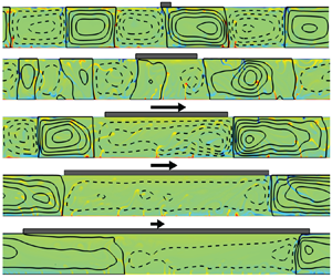
Figure 9. The temporally averaged flow field during the quasi-steady state for the UMM cases in the plate reference frame, for Ra = 5 × 10⁷. From top down, the plate sizes are L = 3, 4, 5, 6, 7, 7.25. The average temperature of the entire flow domain is subtracted from this temporally averaged temperature field, and the residual is denoted as ΔT and is presented by colour. The colour is adjusted to focus on ΔT values within a range of –0.02 to 0.02, and values outside this range are represented by dark blue and red at the ends of the colour bar. The dashed and solid black streamlines represent clockwise and anti-clockwise flow, respectively, with an interval of 500. The thick white line plots the vertically averaged ΔT, denoted by $\overline {\Delta T}$, at different horizontal positions x, with the vertical axis on the right side. The streamline with a value of zero marks the sign-switching positions of the streamfunction.

For the UMM cases, both the temperature anomaly and the streamlines of the time-averaged flow field show that the distance of the hot ‘propelling plume’ away from the plate centre varies with plate size (figure 9). For L = 3, 4, 5, the plume distance increases with plate size L (figure 9a–c). For these cases, the average hot ‘propelling plume’ is located near the trailing edge of the plate, and only a single convection cell is identified underneath the plate (figure 9a–c). For larger plates (L > 5), the hot ‘propelling plume’ is located underneath the plate and shifts toward the centre of the plate as plate size increases (figure 9d–f). As a result, two counter-rotating convection cells are identified underneath the plate, and the dominant one, with a larger contact area at the interface, dictates the direction of plate movement. As plate size L increases from 5 onwards, streamlines show an evident decrease of flow velocity underneath the plate (figure 9), consistent with the decrease of the average plate speed with increasing L over this range of plate size (figure 3b).

The distance of the hot ‘propelling plume’ away from the plate centre is obtained from the time-averaged flow field in two complementary ways, i.e. though the thermal signal and through the momentum signal. First, temperature should decline roughly symmetrically away from the centreline of the hot ‘propelling plume’, and thus the peak position of the vertically averaged temperature profile should represent the position of the plume centreline. Secondly, the streamfunction should switch sign at the centre of the hot ‘propelling plume’, from positive sign (counterclockwise) on the left to negative sign (clockwise) on the right. Therefore, the average sign-switch positions over the entire depth should represent the average plume position.

For cases with a large plate size of L ≥ 6 (figure 9d–f), evident peaks are observed in the vertically averaged temperature profiles, denoted by the white lines in figure 9. For these cases, the hot ‘propelling plume’ is located underneath the plate and the vertically averaged temperature declines roughly symmetrically away from the peak position (figure 9), which represents the centre of the hot plume. Nevertheless, no evident peak with such a symmetrical decline is observed for the smaller plate cases (L = 3, 4, 5) (figure 9a–c), for which the vertically averaged temperature rises abruptly at the trailing edge of the plate and then levels off for a short distance underneath the plate. For these cases, the hot ‘propelling plume’ is located near the edge of the plate. The profile of $\overline {\Delta T}$ for the hot ‘propelling plume’ is severely distorted by the thermal blanket effect of the plate, and therefore the position of the hot ‘propelling plume’ can hardly be identified from the thermal signal. On the other hand, for these cases (L = 3, 4, 5), the streamfunction is observed to switch sign near the trailing edge of the plate, which indicates the presence of a hot plume. Therefore, for these cases (L = 3, 4, 5), the average plume position is determined not from the thermal signal, but from the momentum signal, that is, the position where the streamfunction switches sign. These sign-switch positions do not vary much with depth for the smaller plate cases (L = 3, 4, 5), and thus are averaged vertically to represent the average position of the hot ‘propelling plume’. Nevertheless, an evident deflection of the sign-switch positions is observed near the surface for the large plate cases (L = 6, 7, 7.25). This near-surface deflection results directly from the no-slip boundary condition at the interface, which dictates that the fluid there flows at the same speed as the plate. To avoid this deflection effect, plume distances for the large plate cases (L = 6, 7, 7.25) are determined from the thermal signal, i.e. the peak position of the vertically averaged temperature. Therefore, the thermal signal and the momentum signal are complementary in determining the horizontal position of the hot ‘propelling plume’.

For the UMM cases, the plume distance x ₀ obtained from the average flow field is plotted against the size of the cooling surface, D–L, for two sets of cases with Ra = 10⁶ and Ra = 5 × 10⁷ (figure 10a). Results show that the plume distance x ₀ increases with D–L within a certain range (D–L < 3) and decreases afterwards. The hot ‘propelling plume’ moves horizontally with the unidirectionally moving plate, with an average speed the same as the plate. For the UMM cases, the average plate speed u_p increases with the open surface area (D–L) (figure 10b). Since plate speed u_p is proportional to the plume distance x ₀ ((4.1)), dividing the plate speeds u_p by x ₀ yields values linearly proportional to the open surface area (D–L) (figure 10c). This shows that, for the UMM cases, the average plate speed u_p (or the average horizontally moving speed of the hot ‘propelling plume’) is proportional to x ₀(D–L), expressed as

(4.2)\begin{equation}{u_p} = \alpha {x_0}(D{-}L),\end{equation}

where α is the proportionality coefficient. For a certain Ra, the values of α are almost constant for cases with different plate sizes (figure 10d). The average value of α is 674.49 for Ra = 5 × 10⁷ and 53.25 for Ra = 10⁶. For each Rayleigh number, the difference between the maximum and the minimum values is less than 3 %. Normalizing the quasi-steady-stage time series of plate speed (figure 11a) for different plate sizes by (D–L)x ₀, the normalized time series collapse (figure 11b), confirming this proportionality. The large difference between the α values for the two different Rayleigh numbers (figure 10d) suggests that the value of α depends on Ra. A further investigation at different Ra numbers with a plate size of L = 4 suggests that the coefficient α is proportional to Ra ^0.646 (figure 12).

Figure 10. Plume distance x ₀ (the distance of the hot ‘propelling plume’ away from the plate centre) in the average flow field and the average plate speed u_p for the UMM cases. (a) The variation of x ₀ with the open surface area (D–L). (b) Variation of the average plate speed u_p with the open surface area (D–L). (c) Plate speed u_p divided by plume distance x ₀. (d) Plate speed u_p divided by x ₀(D–L).

Figure 11. (a) Time series of plate speed u_p for different plate sizes L at Ra = 5 × 10⁷ over the quasi-steady stage. (b) Times series normalized by x ₀(D–L), where different time series come together.

Figure 12. The value of α derived from the results of numerical simulations for cases with a plate size of L = 4 for different Rayleigh numbers. The straight line is the result of least square fitting.

5. The critical plate size for the UMM

Results from the numerical simulations suggest that the critical plate size for the UMM lies somewhere between 2.5 and 3.0 (figures 2 and 3a). Here, a simplified cell model is derived to estimate the critical plate size for the UMM. When a moving plate encounters a cold downwelling at its leading edge, it is slowed down by the impeding flow ahead and it takes the cold downwelling along with it (figure 7a,b). During this slowdown process, a cold downwelling is always identified at the leading edge of the plate (Mao et al. Reference Mao, Zhong and Zhang2019). Meanwhile, the hot ‘propelling plume’ behind the plate continues moving ahead, with a speed specified in (4.2). The motion of the plate and the hot ‘propelling plume’ over this slowdown process can be analysed through a simplified cell model (figure 13), which captures the basic flow structure during this slowdown process.

Figure 13. A simplified cell model at the time when the leading edge of the plate encounters a cold downwelling and the associated impeding flow ahead. The red arrow denotes the hot ‘propelling plume’, and the blue arrow represents the cold downwelling at the leading edge of the plate. Cell 1 is the ‘propelling cell’ that propels the plate and cell 2 is the impeding cell that slows down the plate.

With a cold downwelling at the leading edge of the plate, the plate is gradually slowed down by the impeding flow ahead. Since plate speed reflects the average flow speed at the interface, after an infinitesimal time step Δt, the plate speed u_p(t + Δt) can be related to its previous speed u_p(t) as

(5.1)\begin{equation}{u_p}(t + \Delta t) = \frac{1}{L}\{{u_p}(t)[L - {u_p}(t)\varDelta t] - {u_f}(t){u_p}(t)\varDelta t\},\end{equation}

where u_f denotes the average flow speed of the impeding cell (cell 2 in figure 13). Before encountering the cold downwelling, the plate is drifting purely over the propelling cell (cell 1 in figure 13) and its speed reflects the average velocity of the underlying flow, which is roughly the same as u_f. The terms $L - {u_p}(t)\varDelta t$ and ${u_p}(t)\varDelta t$ denote the contact length of the plate with the propelling cell (cell 1 in figure 13) and the impeding cell (cell 2 in figure 13), respectively. Correspondingly, the plate centre position x_p and the hot plume position x_h after an infinitely small time step of Δt are expressed as

(5.2)\begin{gather}{x_p}(t + \Delta t) = {x_p}(t) + {u_p}(t)\varDelta t,\end{gather}

(5.3)\begin{gather}{x_h}(t + \Delta t) = \alpha (D{-}L)[{x_p}(t) - {x_h}(t)]\varDelta t + {x_h}(t),\end{gather}

where the term ${x_p}(t) - {x_h}(t)$ in (5.3) represents the distance of the hot ‘propelling plume’ away from the plate centre, which is denoted as x ₀ in (4.2). Therefore, as specified by (4.2), the term $\alpha (D{-}L)[{x_p}(t) - {x_h}(t)]$ in (5.3) specifies the horizontally moving speed of the hot ‘propelling plume’. The above (5.1)–(5.3) can be expressed in the derivative form as

(5.4)\begin{gather}\frac{{\textrm{d}{u_p}}}{{\textrm{d}t}} ={-} \frac{1}{L}(u_p^2 + {u_f}{u_p}),\end{gather}

(5.5)\begin{gather}\frac{{\textrm{d}{x_p}}}{{\textrm{d}t}} = {u_p},\end{gather}

(5.6)\begin{gather}\frac{{\textrm{d}{x_h}}}{{\textrm{d}t}} = \alpha (D{-}L)[{x_p}(t) - {x_h}(t)].\end{gather}

For the propelling cell (cell 1 in figure 13), mass conservation requires that the vertical mass transport induced by the hot ‘propelling plume’ is equal to the horizontal mass transport away from the plume, i.e.

(5.7)\begin{equation}{v_H}\frac{{{\delta _v}}}{2} = {u_s}{\delta _s}.\end{equation}

Here, v_H is the average vertical speed of the uprising ‘propelling plume’, which is assumed to be roughly symmetrical with a horizontal span of δ_v, and u_s is the average horizontal speed of the surface layer with a thickness of δ_s. Initially, before encountering the cold downwelling, the upper and the lower fluid layers underlying the plate are approximately equally thick with a similar velocity magnitude (for example, figure 14a). As the plate encounters a cold downwelling at its leading edge, it slows down ((5.1)). This slowdown is extended through the viscous drag from the no-slip plate--fluid interface to the interior of the fluid domain, resulting in the decrease of u_s. With a decreasing u_s, mass conservation specified in (5.7) dictates that the surface layer thickens (for example, figure 14b).

Figure 14. Thickening of the surface layer underneath the plate (from (a) to (b)) after the plate's encounter with the cold downwelling. (a) Before the encounter, (b) after the encounter. The black lines are the contours of horizontal velocity, with solid lines for positive velocity and dashed lines for negative velocity.

Nevertheless, the thickness of the surface layer is limited by the depth of the fluid domain h. If u_s has decreased to about half its initial value, the surface layer underneath the plate should expand almost to the entire domain to keep the mass conservation specified in (5.7). If, at this time, the ‘propelling plume’ has not yet reached to the trailing edge of the plate, a further decrease of plate speed without changes in the flow structure would break the rule of mass conservation. Therefore, mass conservation requires a cold downwelling to form between the hot ‘propelling plume’ and the plate to discharge the upper surface flow downwards (figure 6c). In this case, the newly formed cold downwelling blocks the momentum supply from the hot ‘propelling’ plume to the plate, and therefore, the plate is no longer propelled by the underlying fluid and becomes stagnant.

On the other hand, if the ‘propelling plume’ has reached to the trailing edge of the plate, no cold downwelling can form to block the momentum supply from the hot ‘propelling’ plume to the plate, and therefore no stagnation occurs. In this case, nurtured by the thermal blanket, the hot ‘propelling plume’ becomes stronger under the thermal blanket and so does the underlying circulation, pushing the cold downwelling at the leading edge away from the plate. In this way, the plate is no longer slowed down by the impeding flow and soon resumes its speed. Therefore, the critical condition for the unidirectionally moving mode is that the hot ‘propelling plume’ has reached to the trailing edge of the plate before the plate speed decreases to half its initial value, i.e. the value before encountering the cold downwelling.

The above two scenarios are exemplified by the cases with a plate size of L = 1.5 (figure 6a–c) and L = 4 (figure 7c–g), respectively. Although in both cases, a cold downwelling forms behind the plate when the plate is slowed down by the impeding flow ahead, for the former case (L = 1.5), this is accomplished before the establishment of a new hot ‘propelling plume’ at the trailing edge of plate (figure 6c), whereas the reverse is true for the latter case (L = 4.0) (figure 7e). For the latter case (L = 4.0), the transfer of the hot ‘propelling plume’ from the previous one behind the plate to the newly formed one at the trailing edge can be viewed as a horizontal movement of the ‘propelling plume’ with the plate from the long-term perspective. Therefore, the newly formed cold downwelling blocks the momentum supply from the hot ‘propelling plume’ to the plate for the former case, but not for the latter. These different consequences stem from the difference in plate size. The increased plate size enhances the plate's capability to accumulate heat, and therefore enables a faster feedback between the slowdown of the plate and the generation of a new hot ‘propelling plume’.

The time-averaged plate speed is almost constant for plate sizes varying within a range of L = 2 to L = 4 (figure 3b). This is a range that the critical plate size falls into. Since plate speed reflects the average speed of the underlying flow, both the initial plate speed u_p and the speed of the impeding flow u_f are approximated by this constant value. The initial position of the ‘propelling plume’ is determined from (4.2). With these initial conditions, (5.1)–(5.3) are then advanced in time to update the plate speed, and the positions of the plate and the hot ‘propelling plume’ for different plate sizes. Results of the distance of the hot ‘propelling plume’ to the trailing edge of the plate (x_p − L/2 − x_h) and the plate speed u_p are shown in figure 15 for different plate sizes and at different times. It is worth noting that the upper limit of the plate size in this simplified model is set to be 4, since simulation results suggest that the critical plate size for this unidirectional movement is smaller than 4 (figures 2 and 3a). Furthermore, larger plates are associated with a hot ‘propelling plume’ located underneath the plate (figure 9), and thus the present simplified cell model (figure 13) with the hot ‘propelling plume’ located outside the plate coverage no longer applies.

Figure 15. The evolution of the plume distance and the plate velocity with time, derived from (5.1)–(5.3), for different plate sizes at Ra = 5 × 10⁷. (a) The distance of the hot ‘propelling plume’ away from the trailing edge of the plate, x_p − L/2 − x_h. (b) The plate velocity u_p. The transparent horizontal planes in (a) and (b) denote the critical conditions of x_p − L/2 − x_h = 0 (the hot ‘propelling plume’ reaching the trailing edge of the plate) and u_p = u ₀/2 (the plate speed decreasing to half its initial value), respectively. The black lines at the intersection positions mark the critical times for different plate sizes.

It is clear from figure 15b that, as plate size increases, the decrease of plate speed with time occurs at a slower rate, and hence it takes longer time for the plate speed to reduce to half its initial value (black line in figure 15b). Meanwhile, it takes less time for the hot ‘propelling plume’ to reach the trailing edge of the plate as plate size increases (black line in figure 15a). This is largely owing to the fact that, as plate size increases, the hot ‘propelling plume’ is located closer to the edge of the plate (figure 15a), which is consistent with the simulation results (comparing figure 9a with figure 9b). Therefore, it becomes harder for the plate to stop as plate size increases. As discussed above, the two critical conditions for the simplified cell model are:

1. (i) x_p − L/2 − x_h = 0, i.e. the hot ‘propelling plume’ reaches the trailing edge of the plate;

2. (ii) u_p = u ₀/2, i.e. the plate speed u_p decreases to half its initial value.

These two critical conditions are represented by the transparent horizontal planes in figures 15a and 15b, respectively. The critical times at which these two critical conditions are satisfied are denoted as t ₁ and t ₂, respectively, and are marked by the black lines in figure 15. The prerequisite for the occurrence of the UMM is then t ₁ < t ₂, i.e. the hot ‘propelling plume’ has reached the edge of the plate (at time t ₁) before the plate speed reduces to half its initial value (at time t ₂).

For a small plate size of L = 2, t ₁ is larger than t ₂ (figure 16a,b), and therefore stagnancy will occur. In contrast, for a large plate size of L = 4, t ₁ is smaller than t ₂ (figure 16c,d), and hence the plate will move unidirectionally. These predictions are consistent with the results of the full numerical simulations (figure 3). Furthermore, the critical times t ₁ and t ₂ are derived for various plate sizes for both Ra = 10⁶ and Ra = 5 × 10⁷ (figure 17). The critical plate size for the UMM is the size at which t ₁ equals t ₂, or at which t ₁–t ₂ switches sign, from positive to negative as plate size increases (figure 17). Results show that the critical plate size L_c for the UMM decreases with increasing Rayleigh number (from L_c = 3.03 for Ra = 10⁶ to L_c = 2.78 for Ra = 5 × 10⁷).

Figure 16. The distance of the hot ‘propelling plume’ from the edge of the plate (x_p − L/2 − x_h) and the plate velocity u_p, derived from (5.1)–(5.3) for two plate sizes: panels (a,b) are for the case with a plate size of L = 2, for which t ₁ > t ₂ and thus stagnation occurs; and panels (c,d) are for the case with a plate size of L = 4, for which t ₁ < t ₂ and thus the plate moves unidirectionally.

Figure 17. The variation of critical times, t ₁ and t ₂, with plate size L for (a) Ra = 10⁶, (b) Ra = 5 × 10⁷. The variation of t ₁ − t ₂ with L for (c) Ra = 10⁶ and (d) Ra = 5 × 10⁷. The dashed vertical lines denote the critical plate sizes for the UMM.

Since the unidirectionally moving mode is characterized by zero probability of stagnancy (u_p = 0), the probability density of plate speed (figure 18) obtained from the results of full numerical simulations suggests that the transition to the UMM occurs somewhere between L = 3.0 to L = 4.0 for Ra = 10⁶, and between L = 2.5 to L = 3.0 for Ra = 5 × 10⁷. Therefore, the predictions of the critical plate size from the simplified cell model agree well with the results of the full numerical simulations. A comparison between the results for Ra = 10⁶ (figure 18a) and those for Ra = 5 × 10⁷ (figure 18b) shows that the probability of stagnancy decreases with increasing Rayleigh number. For example, for Ra = 10⁶, the plate with a size of L = 3 is still associated with some probability of stagnancy (figure 18a), but for Ra = 5 × 10⁷, its probability of stagnancy vanishes (figure 18b). Therefore, the increase of Rayleigh number enhances the plate's ability to conquer impeding flow and thus decreases the critical plate size for the unidirectionally moving mode.

Figure 18. Probability density of plate speed for (a) Ra = 10⁶ and (b) Ra = 5 × 10⁷. The probability of stagnancy vanishes at a critical place size of somewhere between L = 3 and L = 4 for Ra = 10⁶, and between L = 2.5 and L = 3 for Ra = 5 × 10⁷.

6. The effect of plate size on flow structure

A comparison among the flow structures shown in figure 4 (L = 0.25), figure 5 (L = 0.5), figure 6 (L = 1.5) and figure 7 (L = 4) suggests that, as plate size increases, the number of convection cells within the flow domain decreases. For example, it ranges from 4 to 8 for the case of L = 0.5 in figure 5, but decreases to a range of 2 to 4 for the case of L = 4.0 in figure 7. For a more statistical evaluation, the horizontal profile of the streamfunction is extracted at the middle depth of each snapshot and the number of cells is calculated based on the number of sign-switch positions within the profile. The number of convection cells for each snapshot varies from 2 to 12 and the percentage for each number is shown for each case in figure 19. The number of cells occurs as even numbers since each convection cell is associated with a counter-rotating cell.

Figure 19. The percentage of snapshots composed of the corresponding number of convection cells within the flow domain for cases with different plate size L.

For the very small plate size of L = 0.25, over 90 % of the snapshots are composed of six convection cells (figure 19), agreeing with the flow pattern shown in figure 4. As plate size increases, an increasing percentage of snapshots are composed of less (two or four) convection cells, suggesting that the convection cells are becoming increasingly larger. At the plate size of L = 4.0, over 50 % of the snapshots are composed of only two cells. As plate size increases further to L = 7.0, nearly 100 % of the snapshots are composed of only two convection cells. Therefore, the number of convection cells within the flow domain generally decreases with an increasing plate size.

To reveal the spatial regularity of the flow pattern and its variation with time, the spectra of the streamfunction profile at the middle depth are obtained for each snapshot over a duration of 0.1 (figure 20, the snapshots are saved at a time interval of 3 × 10⁻⁶). For the small plate case of L = 0.25, the spectra are dominated by harmonic degree three most of the time, since the high amplitudes are concentrated on harmonic degree three. This dominance reflects a three-times repetition of the flow structure, and therefore the presence of three hot/cold plumes and six associated convection cells, in agreement with the pattern shown in figure 4. As plate size increases to L = 0.5, the dominant harmonic degree becomes less continuous with time and also more scattered, with a large percentage shifting to the lower values of one and two, and a small percentage shifting to higher values. A further increase of plate size leads to an even less continuous pattern and an enhancing dominance of harmonic degree one. At the very large plate size of L = 7, the spectra become harmonic, with the dominant harmonic degrees being one, three and five. The following analysis will focus on the variation of the spectra with plate size and plate velocity.

Figure 20. Time series of the spectra of the streamfunction profile at the middle depth for different plate size L . From top down, the values of L are 0.25, 0.5, 1, 2, 4 and 7, respectively. The amplitudes of each harmonic degree are indicated by the colour bar.

The temporal average spectra (figure 21) illustrate the enhancing dominance of harmonic degree one (only two convection cells within the flow domain) as plate size increases up to L = 5. This variation indicates that as plate size increases, the flow field orients toward the long-wavelength structure. This is further confirmed by the increasing percentage of snapshots being dominated by harmonic degree one as plate size increases (figure 22a). Therefore, a large plate size favours the formation of large convection cells. For cases with plate size larger than L = 4, all the snapshots are dominated by harmonic degree one and are therefore not shown.

Figure 21. The temporal mean spectra of the streamfunction field over a duration of 0.1 for cases with different plate size L, Ra = 5 × 10⁷. The mean amplitude of the spectra ${\bar{A}_i}$ for each harmonic degree i is normalized by the sum of the amplitudes of all harmonic degrees $\sum\nolimits_{i = 1}^{ + \infty } {{{\bar{A}}_i}}$ (the symbol i denotes positive integers). The mean amplitude of harmonic degree one increases with L up to L = 5. Harmonic wavenumbers emerge at L = 7.0.

Figure 22. (a) Percentage of snapshots dominated by the corresponding harmonic degree. Harmonic degree one dominates an increasing percentage of snapshots as L increases. (b) The average plate speed when the corresponding harmonic degree dominates the spectra. Overall, cases with different L show a general trend of a decreasing average plate speed with an increasing value of the dominant harmonic degree.

The times when each harmonic degree (one to five) dominates the spectra are recorded, and the corresponding plate speeds at those times are averaged (figure 22b). Results show that, for a certain case, an increasing value of the dominant harmonic degree (more convection cells) is generally accompanied with a decreasing plate speed (figure 22b). In other words, a decreasing plate speed corresponds to an increasing number of convection cells or thermal plumes. This trend is confirmed in figure 6 (L = 1.5), as more cells and plumes are identified when the plate is stagnant. This is reasonable as the slowdown of plate is accompanied by the formation of new cold plumes at the trailing edge and new hot plumes underneath the plate (figure 6a–c); in contrast, a velocity burst is accompanied with the coalescence of plumes and the merging of convection cells (figure 6d–f).

The increasing dominance of harmonic degree one with an increasing plate size has been illustrated above for plate sizes up to L = 4 (figure 22a). For an even larger plate, harmonic degree one dominates the spectra almost all the time, and its amplitude, indicating the degree of dominance, varies with time. A strong correlation between its amplitude and the plate speed is suggested by their concurrent time series (figure 23a), with the correlation coefficient larger than 0.8 (figure 23b). This shows that, even for these large plates of L > 4, an increasing plate speed is still accompanied by an enhancing dominance of low harmonic degrees (harmonic degree one for these cases). The above results suggest that an increasing plate speed usually corresponds to an enhancing dominance of longer-wavelength flow structure.

Figure 23. The correlation of plate speed with the amplitude of harmonic degree one. (a) Time series of plate speed (left axis) and the amplitude of harmonic degree one (right axis) for L = 4, Ra = 5 × 10⁷. (b) Plate speed u_p versus the concurrent amplitude of harmonic degree one A ₁ for L = 4 (blue), 6 (orange) and 7 (green). These two values are highly correlated and the correlation coefficient is written with the corresponding colour for each case.