


1. Introduction
The study of starting jets is intrinsically associated with vortex ring formation, as these coherent structures are formed when impulsively pushing fluid from rest through an exhaust. The study of vortex rings gained new momentum after Gharib, Rambod & Shariff (Reference Gharib, Rambod and Shariff1998) showed the existence of an energy optimum during vortex ring formation. More precisely, a non-dimensional time scale, referred as the formation number, was defined as the instant at which the vortex ring starts exhibiting a trailing jet, and was shown to correspond to the stroke ratio required to produce a vortex ring with maximum circulation. An energy-based interpretation of the phenomenon was given by invoking the Kelvin–Benjamin variational principle, which proves the existence of an energy maximum for a given impulse and circulation. Later studies, in a broad range of fields, corroborated this result, hence giving credit to the existence of a universal time scale. For instance, Gharib et al. (Reference Gharib, Rambod, Kheradvar, Sahn and Dabiri2006) showed that blood is expelled in the left ventricle of the human heart in the form of a vortex ring at a stroke ratio of approximately 4. Others, such as Linden & Turner (Reference Linden and Turner2004), Dabiri & Gharib (Reference Dabiri and Gharib2005Reference Dabiri and Ghariba,b) and Dabiri, Colin & Costello (Reference Dabiri, Colin and Costello2006) applied the concept of formation number to fluid transport and propulsion in order to explain and model the locomotion of aquatic animals such as jellyfish and squid (see review by Dabiri Reference Dabiri2009). In particular, it was found that maximum thrust per unit stroke ratio was obtained at this specific formation number value (Krueger & Gharib Reference Krueger and Gharib2003). The potential applications of this concept are broad as the vortex ring is a fundamental coherent structure observable in a wide range of industries. For example, vortex ring thrusters could be potential actuators for unmanned underwater vehicles (Mohseni Reference Mohseni2006; Krieg & Mohseni Reference Krieg and Mohseni2008, Reference Krieg and Mohseni2010), synthetic jets and pulse jets could be used for flow control and mass and heat transfer (see review by Glezer & Amitay Reference Glezer and Amitay2002) and vortex ring-like structures are observed when injecting fuel in a combustion engine (Renard et al. Reference Renard, Thévenin, Rolon and Candel2000).
A growing body of work has shown that the formation number can be affected by specific initial conditions. In particular, the use of a parabolic velocity profile at the exhaust or adding a substantial background co-flow can reduce the value of the formation number to 1 (Rosenfeld, Rambod & Gharib Reference Rosenfeld, Rambod and Gharib1998; Krueger, Dabiri & Gharib Reference Krueger, Dabiri and Gharib2006). On the other hand, adding a bulk counterflow or closing the nozzle while pushing the flow out during formation can increase the formation number up to a value of 8 (Dabiri & Gharib Reference Dabiri and Gharib2004, Reference Dabiri and Gharib2005a). Recently, Limbourg & Nedić (Reference Limbourg and Nedić2021) showed that the use of an orifice geometry results in a reduced formation number of approximately 2, close to the value found by Gao et al. (Reference Gao, Yu, Ai and Law2008) for a gravity-driven gradually converging nozzle and consistent with the observations of Allen & Naitoh (Reference Allen and Naitoh2005). Moreover, care was taken to measure the hydrodynamic impulse and the kinetic energy separately, which led to the definition of additional time scales; a detached vortex ring in a vorticity sense does not necessarily mean that the ring has reached its optimal state, as circulation can be acquired in a discrete fashion by secondary rings catching up with the leading ring. Furthermore, although the ring has detached from the feeding shear layer, the ring can accumulate energy further downstream as the ring has not detached in the velocity sense (Gao & Yu Reference Gao and Yu2010; Limbourg & Nedić Reference Limbourg and Nedić2021). As a consequence, a maximum circulation formation time and an optimal formation time was proposed by Limbourg & Nedić (Reference Limbourg and Nedić2021). Nevertheless, the non-dimensional numbers  $\alpha$,
  $\beta$ and
  $\gamma$ were shown to be adequate quantities to predict the instant at which the ring starts exhibiting a trailing jet, i.e. the formation number.
The difference in the formation process of orifice-generated vortex rings was attributed to the boundary conditions the orifice geometry is imposing. In particular, the radial component of velocity at the exhaust is no longer negligible and must be taken into account in the formation process (Krieg & Mohseni Reference Krieg and Mohseni2013). Moreover, the absence of a boundary layer at the exhaust of the orifice triggers instabilities similar to vortex shedding (Limbourg & Nedić Reference Limbourg and Nedić2021). Finally, the sharp turning angle imposed to the flow by the orifice plate forces the streamlines to bend toward the centreline at the exhaust, hence resulting in a reduced section called vena contracta.
The objective of the present work is to present a correction to the classic slug-flow model which accounts for the contraction of the flow and to investigate its implications for the definition of the formation number. In particular, the model is used to unify results by Limbourg & Nedić (Reference Limbourg and Nedić2021), Krieg & Mohseni (Reference Krieg and Mohseni2013) and Gao et al. (Reference Gao, Yu, Ai and Law2008) with the ones found for a nozzle geometry, for example by Gharib et al. (Reference Gharib, Rambod and Shariff1998).
The structure of the paper is as follows. First, the extended slug-flow model is introduced in § 2. Then, after presenting the experimental setup in § 3, the results are shown in their non-dimensional form in § 4; first as a function of the exhaust-based non-dimensional time  $t^*=U_0 t/D_0$ (§ 4.1), then as a function of the corrected non-dimensional time
  $T^*=U_\star t/D_\star$ (§ 4.2). Finally, a discussion on the formation number and the applicability of the model is given. In particular, a comparison with measurements taken from the literature is furnished.
2. The extended slug-flow model
For an unbounded axisymmetric flow with no swirl, the principal invariants of the motion are the kinetic energy, the hydrodynamic impulse and the circulation:
 \begin{equation} \varGamma = \iint{\omega\,\mathrm{d}r\,\mathrm{d}x}, \quad I = {\rm \pi}\rho \iint{\omega r^2\,\mathrm{d}r\,\mathrm{d}x}, \quad E = {\rm \pi}\rho \iint{\omega \psi\,\mathrm{d}r\,\mathrm{d}x}. \end{equation}
 Given the three integrals of the motion, along with the geometric parameters of the system, it is possible to define three non-dimensional numbers. Taking the circulation and the hydrodynamic impulse to be the repeated variables, the non-dimensional quantities are the stroke ratio  $L/D$ and the non-dimensional numbers
  $\alpha$ and
  $\beta$. Following Linden & Turner (Reference Linden and Turner2001), another non-dimensional number
  $\gamma$ was defined in order to show the importance of the volume (Limbourg & Nedić Reference Limbourg and Nedić2021):
 \begin{equation} \alpha \equiv \frac{E}{\rho^{1/2}\varGamma^{3/2}I^{1/2}},\quad \beta \equiv \frac{\varGamma}{\rho^{{-}1/3}I^{1/3}U^{2/3}},\quad \gamma \equiv \frac{\rlap{-}{V}}{\rho^{{-}3/2}\varGamma^{{-}3/2}I^{3/2}}. \end{equation}
 Naturally, when studying starting jet formation, one must consider the exhaust quantities and thus use the exhaust speed  $U_0$ and discharged volume
  $\rlap{-}{V} _0$ rather than the ring speed
  $U_R$ or the ring volume
  $\rlap{-}{V} _R$.
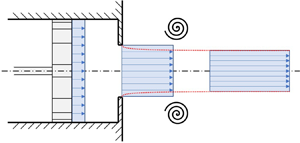
When fluid is pushed out through an orifice, the flow experiences a contraction, and the effective diameter of the column of fluid discharged is reduced (see figure 1). Using the conservation of mass, the geometric quantities (subscript 0) are related to the tube of fluid far downstream (subscript  $\star$) by
 \begin{equation} C_c\equiv A_\star{/}A_0=D_\star^2/D_0^2=L_0/L_\star{=}U_0/U_\star, \end{equation}
where  $C_c$ is the contraction coefficient defined as the ratio of the area of the vena contracta
  $A_\star$, mathematically at infinity downstream, to the area of the orifice
  $A_0$.

Figure 1. Schematic of the slug-flow model made to scale for a unit impulse duration.
As originally shown by Krieg & Mohseni (Reference Krieg and Mohseni2013), the production of the invariants of the motion is drastically influenced by the radial velocity component at the exhaust of the orifice. Krieg & Mohseni (Reference Krieg and Mohseni2013) proposed a semi-empirical model which accounts for the two dimensional effects by fitting the radial velocity and its axial gradient,  $v$ and
  $\partial v/\partial x$, by linear functions. This model was proven to accurately capture the repercussions of the radial velocity on the overall production of circulation, hydrodynamic impulse and kinetic energy. The present model does not aim at modelling precisely the transverse velocity across the exhaust plane, as was done by Krieg & Mohseni (Reference Krieg and Mohseni2013), but rather incorporating its influence on the production of the integrals of the motion. The free streamline theory suggests the contribution of the radial velocity on the velocity profile to be maximum at the edge of the orifice and zero at the centreline. Inversely, the axial velocity is modelled to be zero at the edge of the orifice and maximum at the centreline. The latter is not verified experimentally as shown by Krieg & Mohseni (Reference Krieg and Mohseni2013) and Limbourg & Nedić (Reference Limbourg and Nedić2021). The precise velocity profile at the exhaust assumed by the free streamline theory of Von Mises (Reference Von Mises1917) is unknown. However, accounting for the contraction of the flow allows one to incorporate the effect of the non-zero radial velocity on the flow field by ultimately modelling the discharged column of fluid with a reduced cross section and a greater velocity.
Generally, the rate of production of circulation, hydrodynamic impulse and kinetic energy generated by a parallel starting jet are estimated by the slug-flow model. Introducing the contraction coefficient to account for the reduced section of the flow, the model becomes
 \begin{align} \mathrm{d}\varGamma_{{\star}} = \tfrac{1}{2} U_0^2 \mathrm{d}t \times 1/C_c^2, \quad \mathrm{d}I_{{\star}} = \tfrac{1}{4}{\rm \pi}\rho U_0^2 D_0^2 \mathrm{d}t \times 1/C_c, \quad \mathrm{d}E_{{\star}} = \tfrac{1}{8}{\rm \pi}\rho U_0^3 D_0^2 \mathrm{d}t \times 1/C_c^2 \end{align}
and the predicted non-dimensional numbers  $\alpha$,
  $\beta$ and
  $\gamma$ remain unchanged, as the contraction coefficient cancels out in their expressions:
 \begin{equation} \alpha = \sqrt{\frac{\rm \pi}{2}} \left(\frac{L_0(t)}{D_0}\right)^{{-}1},\quad \beta = \frac{1}{(2{\rm \pi})^{1/3}} \left(\frac{L_0(t)}{D_0}\right)^{2/3},\quad \gamma = \frac{1}{\sqrt{2{\rm \pi}}} \left(\frac{L_0(t)}{D_0}\right). \end{equation}
 Finding the contraction coefficient of a flow is a classical hydrodynamics problem which was first solved by Kirchhoff (Reference Kirchhoff1869), who found the free streamline of a flow exiting an infinitely large vessel through a (rectilinear) two-dimensional slit. The contraction coefficient was found to be  $C_c={\rm \pi} /({\rm \pi} +2)\approx 0.611$. Later, Von Mises (Reference Von Mises1917) provided a thorough study of the two-dimensional problem in a wide variety of boundary conditions, and the contraction coefficient of the sheet of fluid emanating from an infinitely long channel of prescribed width with a two-dimensional conical slot was found. In particular, the case of a
  $90^\circ$ plate covering the exhaust of the channel was found. The equivalent axisymmetric problem of a circular hole in an infinite plane was first solved by Trefftz (Reference Trefftz1916). Later, Rouse & Abul-Fetouh (Reference Rouse and Abul-Fetouh1950) found negligible differences with the two-dimensional results by Von Mises (Reference Von Mises1917) and concluded that the two-dimensional results were applicable to the axisymmetric problem. Consequently, in the present work, the contraction coefficient for different orifice-to-tube ratios is computed using the results of Von Mises (Reference Von Mises1917) and are presented in table 1. For a
  $90^\circ$ angle plate, the contraction coefficient is given by
 \begin{equation} C_c = \frac{\sqrt{h}}{D_0/D_p} \quad \text{with} \ \frac{D_0}{D_p} = \sqrt{h}\left[\frac{2}{\rm \pi}\left(\frac{1}{\sqrt{h}}-\sqrt{h}\right)\arctan\sqrt{h}+1\right], \end{equation}
where  $h$ is a parameter fixing the upstream flow speed.
Table 1. Summary of experimental conditions and contraction coefficients used in the extended slug-flow model (2.6).

The time scale used for studying starting jets and the formation of vortex rings is defined as  $t^*=U_0 t/D_0$ which is equivalent to the instantaneous stroke ratio
  $L_0(t)/D_0$. When accounting for the contraction of the flow, the effective size of the slug of fluid changes and the non-dimensional time becomes
  $T^*=U_\star t/D_\star =U_0 t/D_0\times 1/C_c^{3/2} =t^*\times 1/C_c^{3/2}$. Note that for the case of a nozzle, the contraction coefficient is
  $C_c = 1.000$, and the previously used definition of the time scale is resumed. The latter will be referred as the corrected non-dimensional time.
3. Measurements
Experiments were conducted in a water tank onto which a  $4\ \mathrm {in}=101.6\ \mathrm {mm}$ inner diameter tube was mounted. Several
  $2.38\ \mathrm {mm}$-thick aluminium plates with different orifice diameters were tested, with orifice-to-tube diameter ratios
  $D_0/D_p$ ranging from 0.375 to 1.000, with 0.125 increments, the last case being the straight tube without any plate (see table 1). Water was pushed out by a piston actuator sealed with rubber o-rings. The piston was tuned beforehand in order to avoid spurious overshoots at the end of the acceleration period. The exhaust speed was chosen to be constant for all orifices, hence having a changing diameter-based Reynolds number
  $Re_{D_0}=U_0 D_0/\nu$ (see table 1). In this setting, for a given duration
  $T_0$, the stroke-based Reynolds number
  $Re_{L_0}=U_0 L_0/\nu$ was kept constant. Another set of measurements was taken for a fixed diameter-based Reynolds number of
  $Re_{D_0}=5080$, hence having the targeted speed at the exhaust chosen to be inversely proportional to the orifice diameter. No change in the results was visible; therefore, the presented findings hold for the range of Reynolds number considered here.
Time-resolved planar particle image velocimetry was used to measure the velocity field at the exhaust of the orifice. The field of view extended equally about the axis of symmetry and measurements can be averaged out between the two half-planes. The field of view was adjusted in order to visualise at least two diameters downstream. A total of 15 measurements were taken for every case and the averaged curves are presented in the subsequent figures. Further details on the experimental setup can be found in Limbourg & Nedić (Reference Limbourg and Nedić2021).
4. Results
4.1. Invariants of the motion vs. exhaust-based non-dimensional time  $t^*=U_0 t/D_0$

Figure 2 presents the three non-dimensional numbers  $\alpha$,
  $\beta$ and
  $\gamma$, as defined in (2.2a–c) and measured using particle image velocimetry for the experimental conditions detailed in table 1. First of all, defining the non-dimensional time as
  $t^*=U_0 t/D_0=L_0 (t)/D_0$ enables all slug-flow curves to be collapsed, all being power functions of
  $L_0 (t)/D_0$ (2.5a–c). Figure 2
 $(a)$ presents the non-dimensional number
  $\alpha$, which gathers the three invariants of the motion and which was first introduced by Gharib et al. (Reference Gharib, Rambod and Shariff1998) as an indicator for predicting the formation number. The limiting time was then estimated to be the instant at which the
  $\alpha$ quantity of the steady isolated ring equates the total quantity generated by the apparatus. Several studies have highlighted the importance of this quantity, including Mohseni & Gharib (Reference Mohseni and Gharib1998), Shusser, Gharib & Mohseni (Reference Shusser, Gharib and Mohseni1999), Linden & Turner (Reference Linden and Turner2001), Yu, Law & Ai (Reference Yu, Law and Ai2007), Gao et al. (Reference Gao, Yu, Ai and Law2008), Gao & Yu (Reference Gao and Yu2010) and more recently Gao, Guo & Yu (Reference Gao, Guo and Yu2020) and Steinfurth & Weiss (Reference Steinfurth and Weiss2020). Limbourg & Nedić (Reference Limbourg and Nedić2021) measured the total
  $\alpha$ quantity generated by an orifice geometry having an orifice-to-tube diameter ratio of 0.5, and a clear discrepancy between the measured curve and the slug-flow model prediction was found. As shown in figure 2
 $(a)$, the same is true for other orifice-to-tube diameter ratios, the curves tending towards the slug-flow model as
  $D_0/D_p$ approaches
  $1$. Moreover, for
  $D_0/D_p<0.750$, all experimental curves appear to collapse on each other, and an evident discrepancy is visible between the nozzle case
  $D_0/D_p=1.000$ and the slug-flow model. As suggested by many studies, including Gharib et al. (Reference Gharib, Rambod and Shariff1998) and Gao & Yu (Reference Gao and Yu2010), the
  $\alpha$ quantity is the critical quantity for studying vortex ring formation, and, hypothesizing the
  $\alpha$ quantity of the isolated ring to be 0.33, as found by Gharib et al. (Reference Gharib, Rambod and Shariff1998) for a nozzle geometry or by Limbourg & Nedić (Reference Limbourg and Nedić2021) and Allen & Naitoh (Reference Allen and Naitoh2005) for an orifice geometry, the formation number is found in the range 1.5–2.5, depending on the orifice-to-tube ratio, whilst the intersection with the slug-flow model curve gives a value of 3.8.

Figure 2. Non-dimensional numbers;  $(a)$
$(a)$  $\alpha$ ,
  $(b)$
$(b)$  $\beta$ and
  $(c)$
$(c)$  $\gamma$, as a function of the non-dimensional time
  $t^*$.
The evolution of the non-dimensional number  $\beta$ as a function of the non-dimensional time
  $t^*$ is presented in figure 2
 $(b)$, along with the slug-flow model prediction. The speed
  $U$ in (2.2a–c) is chosen to be the expected exhaust speed
  $U_0$. Again, the slug-flow model is observed to be a mediocre prediction of the non-dimensional number, and all the measurement curves collapse on each other for
  $D_0/D_p<0.750$. For an isolated ring, the
  $\beta$ quantity was measured to be approximately 1.8 for an orifice generated vortex ring (Allen & Naitoh Reference Allen and Naitoh2005; Limbourg & Nedić Reference Limbourg and Nedić2021), close the value of 1.75 for a nozzle geometry (Gharib et al. Reference Gharib, Rambod and Shariff1998; Mohseni & Gharib Reference Mohseni and Gharib1998) or for a converging nozzle (Yu et al. Reference Yu, Law and Ai2007). Given this value, the formation number is found to range from 1.8 to 5.2 for the orifice geometry, whereas following the slug-flow model curve, the formation number would be estimated to be 6.4. Similar comments can be made for
  $\gamma$ (figure 2
 $c$). The
  $\gamma$ quantity for an isolated vortex ring was estimated to be 1.9 by Limbourg & Nedić (Reference Limbourg and Nedić2021), which would give a formation number ranging from 2.0 to 4.0, the latter being for a nozzle geometry (figure 2
 $c$). Again, the formation number would be overestimated by the slug-flow model with a value of 4.8.
4.2. Invariants of the motion vs. corrected non-dimensional time $T^*=U_\star t/D_\star$

The extended slug-flow model, as presented in § 2, is used to predict the non-dimensional quantities and most importantly to redefined the time scale as  $T^\star =U_\star t/D_\star$. While the predicted curves of the non-dimensional numbers remain unchanged, the measured curves are shifted right due to the redefinition of the time scale. The evolution of the non-dimensional numbers
  $\alpha$,
  $\beta$ and
  $\gamma$ is presented as a function of the modified non-dimensional time
  $T^*$ in figure 3. The use of the corrected non-dimensional time collapses all
  $\alpha$ curves, which ultimately follow the slug-flow model. Given the value for an isolated vortex ring of
  $\alpha =0.33$, the formation number is found to range between 2.8 and 3.6 for all orifice-to-tube ratios, and the estimated value using the slug-flow model is 3.8. Similar trends can be observed with the evolution of the
  $\beta$ quantity in figure 3
 $(b)$. Note that the speed used in the definition of
  $\beta$ is
  $U_\star =C_c\times U_0$. Again, all measurement curves collapse on the same curve, close to the extended slug-flow model. The value for an isolated vortex ring was found to be approximately 1.8, which is obtained at a corrected non-dimensional time of
  $T^*=4.6$ to 6.6, 4.6 being for a nozzle geometry. Finally, the
  $\gamma$ quantity is presented in figure 3
 $(c)$. Note that the volume discharged at the exhaust of the orifice is independent of the contraction coefficient, and
  $\rlap{-}{V} _\star =\rlap{-}{V} _0$. Given the
  $\gamma$ quantity of the isolated ring to be approximately 1.9, a formation number of 3.4 and 4.4 is found for all orifices, and a formation number of 4.8 is found with the slug-flow model.

Figure 3. Non-dimensional numbers;  $(a)$
$(a)$  $\alpha$,
  $(b)$
$(b)$  $\beta$ and
  $(c)$
$(c)$  $\gamma$, as a function of the corrected non-dimensional time
  $T^*$.
In short, redefining the non-dimensional time in terms of the contracted quantities unifies the measurements obtained for different tube-to-orifice diameter ratios and tends towards the slug-flow model curve, which is a decent approximation for parallel starting jets.
4.3. Correction for transient effects
Originally, the formation number was defined as the instant at which the vortex ring formed during jet initiation starts exhibiting a trailing jet. The existence of such a limiting time scale was explained by the existence of a maximum energy state, which itself is proven by the Kelvin–Benjamin variational principle. Following Gharib et al. (Reference Gharib, Rambod and Shariff1998), analytical models which involve the three invariants of the motion were proposed to explain and predict the value of the formation number. Making use of the classic slug-flow model for parallel starting jets, on the one hand, and approximating the isolated vortex as a member of the Fraenkel–Norbury family of vortex rings, on the other hand, the formation number was estimated to be 3.0 by Mohseni & Gharib (Reference Mohseni and Gharib1998) and Shusser et al. (Reference Shusser, Gharib and Mohseni1999) and 3.5 by Linden & Turner (Reference Linden and Turner2001). These analytical models proceed to an asymptotic matching of the quantities and discard any transient behaviour. In particular, the slug-flow model assumes a linear increase (in the mathematical sense, i.e. starting from the origin) of the invariants of the motion throughout the formation process, e.g.  $\varGamma _{s}=m_{\varGamma _{s}}t$, where
  $m_{\varGamma _{s}}=1/2U_0^2$. This is not observed experimentally as measurements show a positive offset at
  $t=0$ when applying a linear fit to the curves at a later time (
 $t^*>1$) e.g.
  $\varGamma =m_{\varGamma }t+p_{\varGamma }$. This is attributed to an overpressure effect in the very first instants, as highlighted by Krueger (Reference Krueger2005).
When discarding the transient behaviour by forcing the affine functions to go through the origin, hence only accounting for the rate of production of circulation, impulse and energy, as in the original slug-flow model, the non-dimensional number curves shown in figure 3 become as shown in figure 4. For example,  $\alpha (t) = E(t)\rho ^{-1/2}I(t)^{-1/2}\varGamma (t)^{-3/2} = m_{E}\rho ^{-1/2}m_{I}^{-1/2}m_{\varGamma }^{-3/2} t^{-1}$, where
  $m_{\varGamma }, m_{I}$ and
  $m_{E}$ are the gradients from the measured circulation, impulse and energy curves against time. The use of the corrected non-dimensional time
  $T^*$ clearly enables all
  $\alpha$ curves to be collapsed very close to the slug-flow model curve. In essence, this proves the applicability of the extended slug-flow model for analytical prediction of the formation number for orifice-generated vortex rings. Given an
  $\alpha$ of 0.33 for the isolated ring, a formation number of 3.6–3.8 is found in the modified non-dimensional space (figure 4
 $a$). The nozzle curve differs slightly from the slug-flow model with a formation number of approximately 3.2, which is attributed to the fact that, although a straight nozzle should not experience a contraction of the flow, the presence of a leading vortex and subsequent trailing shear layer forces the flow to contract and modifies the effective shape of the slug of fluid. Moreover, the laminar boundary layer growth inside the tube leads to a reduced diameter of the effective column of fluid at the exhaust which can be accounted for by the present extended slug-flow model; a contraction coefficient of 0.90 would match the nozzle
  $\alpha$ curve with the slug-flow prediction.

Figure 4. Non-dimensional numbers;  $(a)$
$(a)$  $\alpha$,
  $(b)$
$(b)$  $\beta$ and
  $(c)$
$(c)$  $\gamma$, as a function of the corrected non-dimensional time
  $T^*$. Curves corrected for the initial offset.
Figures 4 $(b)$ and 4
 $(c)$ show the evolution of
  $\beta$ and
  $\gamma$, respectively, after correcting for the initial offset. Similar comments can be made. The use of the corrected non-dimensional time brings all the curves together around the slug-flow model curve. Again, the nozzle case is slightly off, and correcting for a contraction of coefficient 0.90 would bring the nozzle curve close to the slug-flow prediction. As highlighted by Limbourg & Nedić (Reference Limbourg and Nedić2021), the use of the non-dimensional numbers
  $\beta$ and
  $\gamma$ with the slug-flow model may lead to an erroneous prediction of the formation number. The
  $\beta$ quantity of 1.8 for the isolated vortex ring would gives a formation number of 6.0–7.2, whereas a
  $\gamma$ quantity of 1.9 for the isolated ring would give a formation number of approximately 5.0 for all orifices.
4.4. Non-dimensionalisation in terms of the ring quantities
A discussion regarding the discrepancy observed here is in order. Unlike the quantity  $\alpha$, which gathers the three integrals of the motion,
  $\beta$ and
  $\gamma$ incorporate the kinematics of the flow via its speed and its volume, respectively. On the one hand, non-dimensional quantities discharged by the apparatus are computed using the targeted exhaust speed
  $U_0$, or equivalent
  $U_\star$, and volume
  $\rlap{-}{V} _0$, or its equivalent
  $\rlap{-}{V} _\star$, and estimated using the slug-flow model. On the other hand, the non-dimensional numbers of the isolated rings are computed using the measured ring speed
  $U_R$ and the measured volume of the ring atmosphere
  $\rlap{-}{V} _R$, independently, regardless of the generating conditions. For this reason, there is no perfect correspondence in the results obtained with the quantity
  $\alpha$ and the quantities
  $\beta$ and
  $\gamma$ when finding the formation number, the latter dimensionless numbers being estimated by the targeted exhaust quantities instead of the ring quantities.
An illustrative example is Hill's spherical vortex, which is the thickest member of the Fraenkel–Norbury family of isolated vortex rings. The non-dimensional numbers are  $\alpha _H=\sqrt {10{\rm \pi} }/35\approx 0.16$,
  $\beta _H=5/(2{\rm \pi} )^{1/3}\approx 2.71$ and
  $\gamma _H=10/3\sqrt {5/2{\rm \pi} }\approx 2.97$, values which would be obtained, if one follows the slug-flow model, at
  $t^*=7.83$,
  $11.18$ and
  $7.45$, respectively. A perfect correspondence in all three numbers is obtained if the exhaust speed
  $U_0$ in the definition of
  $\beta$ is replaced by
  $7/10\times U_0$ and the exhaust volume is replaced by
  $20/21\times \rlap{-}{V} _0$ in the definition of
  $\gamma$. In essence, the total exhaust quantities are now computed in terms of the ring speed and ring diameter, which are not known a priori.
Given the present set of measurements and taking the non-dimensional numbers for the isolated vortex ring to be  $\alpha _R=0.33$,
  $\beta _R=1.8$ and
  $\gamma _R=1.9$ (Limbourg & Nedić Reference Limbourg and Nedić2021), it is possible to compute the equivalent ring quantities which would ultimately give the same prediction for the formation number as the slug-flow model. Replacing the contracted exhaust speed by
  $U_{\star R}=(2\alpha _R\beta _R^{3/2})^{-1}U_\star \approx 0.63U_\star$ and the contracted exhaust volume by
  $\rlap{-}{V} _{\star R}=(2\alpha _R\gamma _R)\rlap{-}{V} _{\star }\approx 1.3\rlap{-}{V} _{\star }$ in figure 4 results in figure 5, and the formation number is found to be 3.80 for all three non-dimensional numbers. Conversely, this also suggests that, given a universal formation time for vortex rings of approximately 4, it is possible to estimate a priori the asymptotic ring speed, volume and diameter, provided the non-dimensional numbers
  $\beta$ and
  $\gamma$ to be universal constants. Note that in figure 5, the measurements taken with the straight nozzle were corrected for the contraction of the flow, and the aforementioned value of 0.90 was used as the contraction coefficient, hence giving a measurement curve close to the theoretical slug-flow curve for all non-dimensional numbers.

Figure 5. Non-dimensional numbers;  $(a)$
$(a)$  $\alpha$,
  $(b)$
$(b)$  $\beta$ and
  $(c)$
$(c)$  $\gamma$, as a function of the corrected non-dimensional time
  $T^*$. Curves corrected for the initial offset.
4.5. Comparison with other measurements
The present model suggests that it is possible to unify the formation number of orifice-generated vortex rings, and this for all orifice-to-tube diameter ratios, with the one obtained for a straight nozzle. The present measurements are compared to data found in the literature in figure 6. In particular, the experimental data of Krieg & Mohseni (Reference Krieg and Mohseni2013) for both the nozzle and the orifice configurations are presented. Note that Krieg & Mohseni (Reference Krieg and Mohseni2013) used a plunger as an actuator and the orifice-to-tube ratio was less than 0.1. Additionally, the data of Gao et al. (Reference Gao, Yu, Ai and Law2008) for a gradually smoothly converging gravity-driven nozzle are shown. Finally, the numerical results of Rosenfeld, Katija & Dabiri (Reference Rosenfeld, Katija and Dabiri2009) for a purely laminar starting jet emanating from a long straight tube at a Reynolds number of 500 are presented. Surprisingly, their  $\alpha$ curve is far from the nozzle measurements – even further from the slug-flow model – and follows the measurements obtained with an orifice geometry (figure 6). This difference is attributed to the very low Reynolds number, which is forming a laminar boundary layer thickness in the nozzle twice as large as in the present nozzle case, hence leading to a reduced slug size at the exhaust. A contraction coefficient of
  $C_c=0.75$ would bring the curve close to the present measurements in the corrected time frame and suggests that the growth of the internal boundary layer plays a key role in the vortex formation mechanism.

Figure 6.  $\alpha$ as a function of
  $(a)$ the non-dimensional time
  $t^*$ and
  $(b)$ the corrected non-dimensional time
  $T^*$.
Krieg & Mohseni (Reference Krieg and Mohseni2013) presented the invariants of the motion in their dimensional form as a function of the dimensional time. Given the information provided, it is possible to present the evolution of  $\alpha$ and
  $\beta$ as a function of the exhaust-based non-dimensional time
  $t^*$. Perfect concordance between the present experimental data and the measurements of Krieg & Mohseni (Reference Krieg and Mohseni2013) is found. In particular, the curve obtained for a straight nozzle differs from the slug-flow model by the same amount. Using a contraction coefficient of
  $C_c=0.611$ for the orifice case of Krieg & Mohseni (Reference Krieg and Mohseni2013), the resulting curves in the corrected non-dimensional time frame
  $T^*$ come closer to the ideal slug-flow model curve. Moreover, using a contraction coefficient of
  $C_c=0.75$ to correct the measurements of Gao et al. (Reference Gao, Yu, Ai and Law2008) obtained for a converging nozzle furnish the same conclusions.
5. Conclusions
Starting jets emanating from orifices with different orifice-to-tube diameter ratios were investigated using particle image velocimetry. The invariants of the motion were measured at the exhaust and presented in their non-dimensional form as a function of the exhaust-based non-dimensional time  $t^*=U_0 t/D_0$. It was found that the classic slug-flow model poorly estimates the production of the invariants of the motion, especially for small orifice-to-tube diameter ratios. This is corroborated by previous studies by Krieg & Mohseni (Reference Krieg and Mohseni2013) and Limbourg & Nedić (Reference Limbourg and Nedić2021). A correction to the slug-flow model was proposed to account for the contraction of the flow at the exhaust and was shown to collapse all experimental curves together. Moreover, discarding the transient effects and only accounting for the rate of production of the invariants of the motion, as in the classic slug-flow model, confirms that the corrected non-dimensional time
  $T^*=U_\star t/D_\star$ collapses all experimental curves together, close to the slug-flow model. Although, theoretically, no correction should be applied to the straight nozzle case, it is found that a contraction coefficient of 0.90 would unify all curves to the slug-flow model, including the nozzle case, for the present experimental conditions. This proves that it is possible to extend the analytical predictions of the formation number of Mohseni & Gharib (Reference Mohseni and Gharib1998), Shusser et al. (Reference Shusser, Gharib and Mohseni1999) and Linden & Turner (Reference Linden and Turner2001) to orifice-generated vortex rings.
Using an  $\alpha$ value of 0.33 for the isolated vortex ring, the formation number, defined as the corrected non-dimensional time
  $T^*$ at which the total curve reaches this value, is found to range between 2.8 and 3.6, consistent with analytical predictions of Mohseni & Gharib (Reference Mohseni and Gharib1998), Linden & Turner (Reference Linden and Turner2001) or Shusser et al. (Reference Shusser, Gharib and Mohseni1999) and slightly lower than the value found for a nozzle geometry by Gharib et al. (Reference Gharib, Rambod and Shariff1998) using circulation alone. Nevertheless, this must be seen in the context of the original formation number of 1.5–2.5 found for orifice-generated vortex rings using the exhaust-based non-dimensional time
  $t^*$. Furthermore, correcting for the transient effects shows that the theoretical formation number would be 3.8 for all cases. The
  $\beta$ quantity was also used to estimate the formation number and, given a
  $\beta$ of approximately 1.8–2.0 for the isolated ring, a formation number of 1.8–5.5 was found using the experimental curves in the exhaust-based non-dimensional time frame. Using the corrected non-dimensional time enables to unify the results with a formation number found around 6.5. The difference to the value found for
  $\alpha$ was reported by Limbourg & Nedić (Reference Limbourg and Nedić2021) and remains an open question. Similar conclusions can be made regarding
  $\gamma$, which gives a formation number in the range of 2.4–4.4.
Finally, the extended slug-flow model and the redefinition of the non-dimensional time were tested on the experimental data of Krieg & Mohseni (Reference Krieg and Mohseni2013) and Gao et al. (Reference Gao, Yu, Ai and Law2008). The results show a perfect agreement with the present set of data. The use of the corrected model therefore enables the unification of the formation number found for vortex rings emanating from orifice geometries and converging nozzles with the common result of Gharib et al. (Reference Gharib, Rambod and Shariff1998) for straight nozzles.
Funding
Financial supports from the Natural Sciences and Engineering Research Council of Canada and the Fonds de Recherche du Québec Nature et Technologie are gratefully acknowledged.
Declaration of interests
The authors report no conflict of interest.


