2.1 Remarks on the boundary conditions for practical applications

In this work, the velocity of the incoming gust is assumed to be the same as in the far field, i.e. the following representation of the gust in the theoretical application is used:

(2.5) $$\begin{eqnarray}\boldsymbol{v}_{g}^{\prime }(\boldsymbol{x},t)=(u_{g}^{\prime },v_{g}^{\prime })=(-k_{2},k_{1})\frac{A_{v}}{\sqrt{k_{1}^{2}+k_{2}^{2}}}\exp (\text{i}\unicode[STIX]{x1D714}t-\text{i}k_{1}x_{1}-\text{i}k_{2}x_{2}),\quad \unicode[STIX]{x1D714}=k_{1}u_{\infty }.\end{eqnarray}$$

However, in practical situations, the gust experiences distortion by the non-uniform mean flow; the value of $\boldsymbol{v}_{g}^{\prime }$ should gradually differ from (2.5). One consequence of the gust distortion is that the turbulence statistics (for the broadband case) might be altered, as has been studied in the previous works by Moreau et al. (Reference Moreau, Roger and Jurdic2005), Christophe et al. (Reference Christophe, Anthoine and Moreau2009), Christophe (Reference Christophe2011) and Santana et al. (Reference Santana, Christophe, Schram and Desmet2016). In this case, one possible approach to account for this effect is to use the theory by Goldstein (Reference Goldstein1978) that considers the distortion of the gusts. Atassi & Grzedzinski (Reference Atassi and Grzedzinski1989) modified Goldstein’s formulation to remove the singularity, and the method was employed by Scott & Atassi (Reference Scott and Atassi1990) for numerical calculation. However, the problem in using the modified method is that the boundary condition ahead of the airfoil ( $\unicode[STIX]{x1D719}=0$ when $x_{1}<0$ ) is not given, making it difficult to solve the equation analytically. Any numerical approach to solve (2.1) should be conducted in the 2-D domain. Therefore, the analytical study proposed in this work should be viewed as a correction method to the flat-plate solution rather than an exact solution for real airfoils.

2.2 Analytical solution

2.2.1 Sound governing equation in the transformed coordinates

To account for the effect of background mean flow on the acoustic process, a coordinate transformation is introduced in the general form

(2.6a-c ) $$\begin{eqnarray}X_{1}=F(x_{1}),\quad X_{2}=G(x_{2}),\quad T=\unicode[STIX]{x1D702}t+\unicode[STIX]{x1D6F9}(x_{1},x_{2}).\end{eqnarray}$$

The following relationships can be obtained:

(2.7a-c ) $$\begin{eqnarray}\frac{\unicode[STIX]{x2202}}{\unicode[STIX]{x2202}x_{1}}=f(x_{1})\frac{\unicode[STIX]{x2202}}{\unicode[STIX]{x2202}X_{1}}+\unicode[STIX]{x1D6F9}_{1}\frac{\unicode[STIX]{x2202}}{\unicode[STIX]{x2202}T},\quad \frac{\unicode[STIX]{x2202}}{\unicode[STIX]{x2202}x_{2}}=g(x_{2})\frac{\unicode[STIX]{x2202}}{\unicode[STIX]{x2202}X_{2}}+\unicode[STIX]{x1D6F9}_{2}\frac{\unicode[STIX]{x2202}}{\unicode[STIX]{x2202}T},\quad \frac{\unicode[STIX]{x2202}}{\unicode[STIX]{x2202}t}=\unicode[STIX]{x1D702}\frac{\unicode[STIX]{x2202}}{\unicode[STIX]{x2202}T},\end{eqnarray}$$

where $f(x_{1})=F^{\prime }(x_{1})$ , $g(x_{2})=G^{\prime }(x_{2})$ , $\unicode[STIX]{x1D6F9}_{1}=\unicode[STIX]{x2202}\unicode[STIX]{x1D6F9}/\unicode[STIX]{x2202}x_{1}$ and $\unicode[STIX]{x1D6F9}_{2}=\unicode[STIX]{x2202}\unicode[STIX]{x1D6F9}/\unicode[STIX]{x2202}x_{2}$ . When the background mean flow is uniform, the governing equation is the convected wave equation, which can be reduced to a classical wave equation by using the Prandtl–Glauert transformation: $X_{1}=x_{1}/\unicode[STIX]{x1D6FD}_{\infty }$ , $X_{2}=x_{2}$ and $T=\unicode[STIX]{x1D6FD}_{\infty }t+M_{\infty }x_{1}/(a_{\infty }\unicode[STIX]{x1D6FD}_{\infty })$ . In this case $f=1/\unicode[STIX]{x1D6FD}_{\infty }$ , $g=1$ , $\unicode[STIX]{x1D702}=\unicode[STIX]{x1D6FD}_{\infty }$ , $\unicode[STIX]{x2202}\unicode[STIX]{x1D6F9}/\unicode[STIX]{x2202}x_{1}=M_{\infty }/(a_{\infty }\unicode[STIX]{x1D6FD}_{\infty })$ and $\unicode[STIX]{x2202}\unicode[STIX]{x1D6F9}/\unicode[STIX]{x2202}x_{2}=0$ . The factor $\unicode[STIX]{x1D6FD}_{\infty }$ is introduced to account for the convection effect by the streamwise uniform mean flow. However, large errors exist in practical applications with non-uniform mean flow, which motivates this work. To tackle the problem, we develop a generalised space–time transformation that is analogous to the Prandtl–Glauert transformation. The coefficients in the space–time transformation are determined by the local flow variables

(2.8a-c ) $$\begin{eqnarray}X_{1}=\int _{{\mathcal{L}}}\frac{\text{d}\unicode[STIX]{x1D709}_{1}}{\unicode[STIX]{x1D6FD}_{1}(\unicode[STIX]{x1D743})},\quad X_{2}=\int _{{\mathcal{L}}}\frac{\text{d}\unicode[STIX]{x1D709}_{2}}{\unicode[STIX]{x1D6FD}_{2}(\unicode[STIX]{x1D743})},\quad T=\unicode[STIX]{x1D6FD}_{\infty }t+\unicode[STIX]{x1D6F9}.\end{eqnarray}$$

Here the notation $(\cdot )_{{\mathcal{L}}}$ means that the integrations are performed along the streamline ${\mathcal{L}}$ from $\unicode[STIX]{x1D743}=\mathbf{0}$ to $\unicode[STIX]{x1D743}=(x_{1},x_{2})$ , $\unicode[STIX]{x1D6FD}_{1}=\sqrt{1-M_{1}^{2}}$ , $\unicode[STIX]{x1D6FD}_{2}=\sqrt{1-M_{2}^{2}}$ , $M_{1}(\boldsymbol{x})=u_{1}(\boldsymbol{x})/a_{0}(\boldsymbol{x})$ and $M_{2}(\boldsymbol{x})=u_{2}(\boldsymbol{x})/a_{0}(\boldsymbol{x})$ are the local Mach numbers, and

(2.9a,b ) $$\begin{eqnarray}\frac{\unicode[STIX]{x2202}\unicode[STIX]{x1D6F9}}{\unicode[STIX]{x2202}x_{1}}=\frac{M_{1}}{\unicode[STIX]{x1D6FD}_{1}a_{0}},\quad \frac{\unicode[STIX]{x2202}\unicode[STIX]{x1D6F9}}{\unicode[STIX]{x2202}x_{2}}=\frac{M_{2}}{\unicode[STIX]{x1D6FD}_{2}a_{0}}\quad \Rightarrow \quad \unicode[STIX]{x1D6F9}(x_{1},x_{2})=\int _{{\mathcal{L}}}\left[\frac{\unicode[STIX]{x2202}\unicode[STIX]{x1D6F9}}{\unicode[STIX]{x2202}\unicode[STIX]{x1D709}_{1}}\text{d}\unicode[STIX]{x1D709}_{1}+\frac{\unicode[STIX]{x2202}\unicode[STIX]{x1D6F9}}{\unicode[STIX]{x2202}\unicode[STIX]{x1D709}_{2}}\text{d}\unicode[STIX]{x1D709}_{2}\right].\end{eqnarray}$$

One can then obtain that

(2.10a-c ) $$\begin{eqnarray}f(\boldsymbol{x})=\frac{1}{\unicode[STIX]{x1D6FD}_{1}(\boldsymbol{x})},\quad g(\boldsymbol{x})=\frac{1}{\unicode[STIX]{x1D6FD}_{2}(\boldsymbol{x})},\quad \unicode[STIX]{x1D702}=\unicode[STIX]{x1D6FD}_{\infty }.\end{eqnarray}$$

Equations (2.8) can be viewed as a generalisation of the Prandtl–Glauert transformation where the coefficients $\unicode[STIX]{x1D6FD}_{\infty }$ and $M_{\infty }$ are replaced by the non-uniform ones $\unicode[STIX]{x1D6FD}_{1}$ , $\unicode[STIX]{x1D6FD}_{2}$ , $M_{1}$ and $M_{2}$ . An integration along the streamline is used to account for the dependence of the new coordinate variables $\boldsymbol{X}$ on the original one $\boldsymbol{x}$ . With the new transformation, the following classical wave equation is solved in the transformed domain:

(2.11) $$\begin{eqnarray}\frac{\unicode[STIX]{x2202}^{2}\unicode[STIX]{x1D719}}{\unicode[STIX]{x2202}T^{2}}-a_{0}^{2}\left(\frac{\unicode[STIX]{x2202}^{2}\unicode[STIX]{x1D719}}{\unicode[STIX]{x2202}X_{1}^{2}}+\frac{\unicode[STIX]{x2202}^{2}\unicode[STIX]{x1D719}}{\unicode[STIX]{x2202}X_{2}^{2}}\right)=\mathscr{E}.\end{eqnarray}$$

To obtain the solution, usually we need to omit $\mathscr{E}$ , which is the approximation error due to the space–time transformation. The dependence of $\mathscr{E}$ on the flow speed is analysed in appendix A. In general, the magnitude of the errors for most terms are $O(M_{\infty }^{2})$ or $O(M_{\infty }^{3})$ , while the error of the time derivative $\unicode[STIX]{x2202}\unicode[STIX]{x1D719}/\unicode[STIX]{x2202}T$ is $O(M_{\infty })$ , suggesting that there could be larger errors at higher frequencies at higher Mach numbers. In the theoretical analysis, we can assume that the variables are time harmonic such that

(2.12) $$\begin{eqnarray}\unicode[STIX]{x1D719}(\boldsymbol{x},t)=\hat{\unicode[STIX]{x1D719}}(\boldsymbol{x})\text{e}^{\text{i}\unicode[STIX]{x1D714}t}=\hat{\unicode[STIX]{x1D719}}(\boldsymbol{x})\exp \left[\frac{\text{i}\unicode[STIX]{x1D714}(T-\unicode[STIX]{x1D6F9})}{\unicode[STIX]{x1D702}}\right]=\unicode[STIX]{x1D711}(\boldsymbol{X})\text{e}^{\text{i}\unicode[STIX]{x1D6FA}T},\end{eqnarray}$$

where $\unicode[STIX]{x1D714}$ is the angular frequency in the original space, while $\unicode[STIX]{x1D6FA}=\unicode[STIX]{x1D714}/\unicode[STIX]{x1D702}$ is the angular frequency in the transformed domain, i.e. the variables have a time dependence $\text{e}^{\text{i}\unicode[STIX]{x1D6FA}T}$ and the amplitudes in the two domains are related by

(2.13) $$\begin{eqnarray}\unicode[STIX]{x1D711}(\boldsymbol{X})=\hat{\unicode[STIX]{x1D719}}(\boldsymbol{x})\text{e}^{-\text{i}\unicode[STIX]{x1D6FA}\unicode[STIX]{x1D6F9}}.\end{eqnarray}$$

The same relation is also applicable for other variables. Now we consider representations of the boundary conditions in the transformed domain. In the region ahead of the airfoil, it is straightforward to obtain that

(2.14) $$\begin{eqnarray}\unicode[STIX]{x1D711}(X_{1},0)=0,\quad \text{for }X_{1}<0.\end{eqnarray}$$

Similarly, the boundary condition in the wake region is written as

(2.15) $$\begin{eqnarray}\tilde{p}(\boldsymbol{X})=0,\quad \text{for }X_{1}>C,\end{eqnarray}$$

where $\tilde{p}$ is the spatial part of the sound pressure written in the transformed domain. On the airfoil surface $0\leqslant X_{1}\leqslant C$ , the hard-wall condition (2.4) is

(2.16) $$\begin{eqnarray}\displaystyle & & \displaystyle w=n_{1}\frac{\unicode[STIX]{x2202}\unicode[STIX]{x1D719}}{\unicode[STIX]{x2202}x_{1}}+n_{2}\frac{\unicode[STIX]{x2202}\unicode[STIX]{x1D719}}{\unicode[STIX]{x2202}x_{2}}=\left(n_{1}\frac{\unicode[STIX]{x2202}\unicode[STIX]{x1D6F9}}{\unicode[STIX]{x2202}x_{1}}+n_{2}\frac{\unicode[STIX]{x2202}\unicode[STIX]{x1D6F9}}{\unicode[STIX]{x2202}x_{2}}\right)\frac{\unicode[STIX]{x2202}\unicode[STIX]{x1D719}}{\unicode[STIX]{x2202}T}+n_{1}f\frac{\unicode[STIX]{x2202}\unicode[STIX]{x1D719}}{\unicode[STIX]{x2202}X_{1}}+n_{2}g\frac{\unicode[STIX]{x2202}\unicode[STIX]{x1D719}}{\unicode[STIX]{x2202}X_{2}},\nonumber\\ \displaystyle & & \displaystyle \quad \Rightarrow \quad \frac{\unicode[STIX]{x2202}\unicode[STIX]{x1D719}}{\unicode[STIX]{x2202}X_{2}}=\frac{1}{n_{2}g}\left[w-\left(n_{1}\frac{\unicode[STIX]{x2202}\unicode[STIX]{x1D6F9}}{\unicode[STIX]{x2202}x_{1}}+n_{2}\frac{\unicode[STIX]{x2202}\unicode[STIX]{x1D6F9}}{\unicode[STIX]{x2202}x_{2}}\right)\frac{\unicode[STIX]{x2202}\unicode[STIX]{x1D719}}{\unicode[STIX]{x2202}T}-n_{1}f\frac{\unicode[STIX]{x2202}\unicode[STIX]{x1D719}}{\unicode[STIX]{x2202}X_{1}}\right].\end{eqnarray}$$

With the time-dependent term $\text{e}^{\text{i}\unicode[STIX]{x1D6FA}T}$ omitted, the condition can be represented as

(2.17) $$\begin{eqnarray}\frac{\unicode[STIX]{x2202}\unicode[STIX]{x1D711}}{\unicode[STIX]{x2202}X_{2}}=\tilde{W}(\boldsymbol{x})\triangleq \frac{1}{n_{2}g}\left[W-\text{i}\unicode[STIX]{x1D6FA}\left(n_{1}\frac{\unicode[STIX]{x2202}\unicode[STIX]{x1D6F9}}{\unicode[STIX]{x2202}x_{1}}+n_{2}\frac{\unicode[STIX]{x2202}\unicode[STIX]{x1D6F9}}{\unicode[STIX]{x2202}x_{2}}\right)\unicode[STIX]{x1D711}-n_{1}f\frac{\unicode[STIX]{x2202}\unicode[STIX]{x1D711}}{\unicode[STIX]{x2202}X_{1}}\right],\quad \text{for }0\leqslant X_{1}\leqslant C,\end{eqnarray}$$

where $W(\boldsymbol{X})={\hat{w}}(\boldsymbol{x})\exp (-\text{i}\unicode[STIX]{x1D6FA}\unicode[STIX]{x1D6F9})$ and ${\hat{w}}$ is the spatially dependent part of $w(\boldsymbol{x},t)$ defined in (2.4), i.e. $w(\boldsymbol{x},t)=W(\boldsymbol{X})\text{e}^{\text{i}\unicode[STIX]{x1D6FA}T}$ .

In summary, with the term $\mathscr{E}$ omitted, the equivalent Helmholtz equation to solve in the new coordinates is

(2.18) $$\begin{eqnarray}{\mathcal{K}}^{2}\unicode[STIX]{x1D711}+\left(\frac{\unicode[STIX]{x2202}^{2}\unicode[STIX]{x1D711}}{\unicode[STIX]{x2202}X_{1}^{2}}+\frac{\unicode[STIX]{x2202}^{2}\unicode[STIX]{x1D711}}{\unicode[STIX]{x2202}X_{2}^{2}}\right)=0,\quad {\mathcal{K}}=\frac{\unicode[STIX]{x1D6FA}}{a_{\infty }},\end{eqnarray}$$

where $\unicode[STIX]{x1D6FA}=\unicode[STIX]{x1D714}/\unicode[STIX]{x1D6FD}$ , and $\unicode[STIX]{x1D711}$ is the spatially varying part of the velocity potential in the transformed domain, which is defined in (2.12) and (2.13). The boundary conditions in different regions of the streamline ${\mathcal{L}}$ are

(2.19) $$\begin{eqnarray}\left.\begin{array}{@{}c@{}}\displaystyle \unicode[STIX]{x1D711}(\boldsymbol{X})=0,\quad X_{1}<0,\\ \displaystyle \frac{\unicode[STIX]{x2202}\unicode[STIX]{x1D711}(\boldsymbol{X})}{\unicode[STIX]{x2202}X_{2}}=\tilde{W}(\boldsymbol{X}),\quad 0\leqslant X_{1}\leqslant C,\\ \displaystyle \tilde{p}(\boldsymbol{X})=0,\quad X_{1}>C.\end{array}\right\}\end{eqnarray}$$

Having obtained the (approximate) classical wave equation, which is the main contribution of this paper, the Schwarzschild technique (Schwarzschild Reference Schwarzschild1901) is used to obtain the solution of pressure fluctuation on the airfoil surface. The procedures are similar to that given in Amiet (Reference Amiet1976a ), but with some slight modifications due to the non-uniformities of the mean flow variables. The details are provided in the next section for completeness. When the pressure fluctuation on the airfoil surface is computed, the Kirchhoff–Helmholtz integral, which is equivalent to Curle’s acoustic analogy (Curle Reference Curle1955; Christophe Reference Christophe2011) for this problem, is applied to compute the sound distribution at the given observers (that are often in the far field).

In the solution, we need to compute the relationship between the pressure fluctuation $p(\boldsymbol{x},t)$ and velocity potential $\unicode[STIX]{x1D719}(\boldsymbol{x},t)$ in the transformed domain. From (2.2) and (2.7), the two variables are related by

(2.20) $$\begin{eqnarray}-\frac{p}{\unicode[STIX]{x1D70C}_{0}}=\frac{\text{D}_{0}\unicode[STIX]{x1D719}}{\text{D}t}=\left[\left(\unicode[STIX]{x1D702}+u_{1}\frac{\unicode[STIX]{x2202}\unicode[STIX]{x1D6F9}}{\unicode[STIX]{x2202}x_{1}}+u_{2}\frac{\unicode[STIX]{x2202}\unicode[STIX]{x1D6F9}}{\unicode[STIX]{x2202}x_{2}}\right)\frac{\unicode[STIX]{x2202}}{\unicode[STIX]{x2202}T}+u_{1}f\frac{\unicode[STIX]{x2202}}{\unicode[STIX]{x2202}X_{1}}+u_{2}g\frac{\unicode[STIX]{x2202}}{\unicode[STIX]{x2202}X_{2}}\right]\unicode[STIX]{x1D719}.\end{eqnarray}$$

The difficulty in using this equation is that the value of $\unicode[STIX]{x2202}\unicode[STIX]{x1D719}/\unicode[STIX]{x2202}X_{2}$ may depend on the transverse coordinate $X_{2}$ , while all integration and differential calculations are performed along the streamline in the analytical derivations. Therefore, we need to replace this term with functions that depend only on $X_{1}$ . For simplicity, equation (2.20) is denoted as

(2.21) $$\begin{eqnarray}\tilde{p}=-\unicode[STIX]{x1D70C}_{0}\left[\left(\text{i}\unicode[STIX]{x1D6FA}\unicode[STIX]{x1D6E4}+\unicode[STIX]{x1D6E9}\frac{\unicode[STIX]{x2202}}{\unicode[STIX]{x2202}X_{1}}\right)\unicode[STIX]{x1D711}+\mathscr{T}\right].\end{eqnarray}$$

In the regions ahead of the airfoil leading edge and after the airfoil trailing edge, we assume that $\unicode[STIX]{x2202}\unicode[STIX]{x1D719}/\unicode[STIX]{x2202}X_{2}$ is small such that

(2.22a-c ) $$\begin{eqnarray}\unicode[STIX]{x1D6E4}=\unicode[STIX]{x1D702}+u_{1}\frac{\unicode[STIX]{x2202}\unicode[STIX]{x1D6F9}}{\unicode[STIX]{x2202}x_{1}}+u_{2}\frac{\unicode[STIX]{x2202}\unicode[STIX]{x1D6F9}}{\unicode[STIX]{x2202}x_{2}},\quad \unicode[STIX]{x1D6E9}=u_{1}f,\quad \mathscr{T}=0,\quad \text{for }X_{1}<0\text{ or }X_{1}>C.\end{eqnarray}$$

On the airfoil surface ( $0\leqslant X_{1}\leqslant C$ ), a combination of (2.17) and (2.20) yields

(2.23) $$\begin{eqnarray}\unicode[STIX]{x1D6E4}=\unicode[STIX]{x1D702}+u_{1}\frac{\unicode[STIX]{x2202}\unicode[STIX]{x1D6F9}}{\unicode[STIX]{x2202}x_{1}}+u_{2}\frac{\unicode[STIX]{x2202}\unicode[STIX]{x1D6F9}}{\unicode[STIX]{x2202}x_{2}}-\frac{u_{2}}{n_{2}}\left(n_{1}\frac{\unicode[STIX]{x2202}\unicode[STIX]{x1D6F9}}{\unicode[STIX]{x2202}x_{1}}+n_{2}\frac{\unicode[STIX]{x2202}\unicode[STIX]{x1D6F9}}{\unicode[STIX]{x2202}x_{2}}\right)=\unicode[STIX]{x1D702}+\left(\frac{u_{1}n_{2}-u_{2}n_{1}}{n_{2}}\right)\frac{\unicode[STIX]{x2202}\unicode[STIX]{x1D6F9}}{\unicode[STIX]{x2202}x_{1}}.\end{eqnarray}$$

By introducing a new variable $V=u_{1}n_{2}-u_{2}n_{1}$ , which is the flow velocity along the streamline, we can compute $\unicode[STIX]{x1D6E4}$ , $\unicode[STIX]{x1D6E9}$ and $\mathscr{T}$ as

(2.24a-c ) $$\begin{eqnarray}\unicode[STIX]{x1D6E4}=\unicode[STIX]{x1D702}+\frac{V}{n_{2}}\frac{\unicode[STIX]{x2202}\unicode[STIX]{x1D6F9}}{\unicode[STIX]{x2202}x_{1}},\quad \unicode[STIX]{x1D6E9}=\frac{f\,V}{n_{2}},\quad \mathscr{T}=\frac{\tilde{W}u_{2}}{n_{2}},\quad \text{for }0\leqslant X_{1}\leqslant C.\end{eqnarray}$$

Equation (2.21) suggests that the sound pressure $\tilde{p}$ (or $p$ in the original domain) can be computed from the known value of $\unicode[STIX]{x1D711}(\boldsymbol{X})$ . Conversely, $\unicode[STIX]{x1D711}$ can also be solved from the known value of $\tilde{p}$ based on the ordinary differential equation (ODE)

(2.25) $$\begin{eqnarray}\frac{\unicode[STIX]{x2202}\unicode[STIX]{x1D711}}{\unicode[STIX]{x2202}X_{1}}+a(X_{1})\unicode[STIX]{x1D711}=b(X_{1}),\end{eqnarray}$$

where the coefficients are determined from (2.21):

(2.26a,b ) $$\begin{eqnarray}a(X_{1})=\frac{\text{i}\unicode[STIX]{x1D6FA}\unicode[STIX]{x1D6E4}}{\unicode[STIX]{x1D6E9}},\quad b(X_{1})=-\frac{1}{\unicode[STIX]{x1D6E9}}\left(\frac{\tilde{p}}{\unicode[STIX]{x1D70C}_{0}}+\mathscr{T}\right).\end{eqnarray}$$

Then the solution to this ODE is (cf. section 2.4 in Goodwine (Reference Goodwine2010)):

(2.27) $$\begin{eqnarray}\unicode[STIX]{x1D711}(X_{1})=\frac{{\mathcal{F}}_{1}(X_{1})}{{\mathcal{F}}_{2}(X_{1})},\quad \text{where }\left.\begin{array}{@{}c@{}}\displaystyle {\mathcal{F}}_{1}(X_{1})=\int _{-\infty }^{X_{1}}b(\unicode[STIX]{x1D709})\exp \left(\int _{-\infty }^{\unicode[STIX]{x1D709}}a(\unicode[STIX]{x1D702})\,\text{d}\unicode[STIX]{x1D702}\right)\,\text{d}\unicode[STIX]{x1D709},\\ \displaystyle {\mathcal{F}}_{2}(X_{2})=\exp \left(\int _{-\infty }^{X_{1}}a(\unicode[STIX]{x1D709})\,\text{d}\unicode[STIX]{x1D709}\right).\end{array}\right\}\end{eqnarray}$$

2.2.2 Solution using the Schwarzschild technique

The Schwarzschild solution is used to compute the pressure fluctuation on the airfoil surface, which will then be used for the computation of the sound pressure at the observer points elsewhere. Usually, the Schwarzschild solution is valid for the Helmholtz equation with two-section semi-infinite mixed boundary conditions (Schwarzschild Reference Schwarzschild1901; Amiet Reference Amiet1976a )

(2.28a,b ) $$\begin{eqnarray}\unicode[STIX]{x1D735}_{X}^{2}\unicode[STIX]{x1D711}+{\mathcal{K}}^{2}\unicode[STIX]{x1D711}=0,\quad \unicode[STIX]{x1D711}(X_{1},0)=F(X_{1}),\quad \text{for }X_{1}\geqslant 0;\quad \frac{\unicode[STIX]{x2202}\unicode[STIX]{x1D711}}{\unicode[STIX]{x2202}X_{2}}=0,\quad \text{for }X_{1}<0.\end{eqnarray}$$

Then the solution for any $X_{1}<0$ is

(2.29) $$\begin{eqnarray}\unicode[STIX]{x1D711}(X_{1},0)=\frac{1}{\unicode[STIX]{x03C0}}\int _{0}^{\infty }\sqrt{\frac{-X_{1}}{\unicode[STIX]{x1D709}}}\frac{\text{e}^{-\text{i}{\mathcal{K}}(\unicode[STIX]{x1D709}-X_{1})}}{\unicode[STIX]{x1D709}-X_{1}}F(\unicode[STIX]{x1D709})\,\text{d}\unicode[STIX]{x1D709}.\end{eqnarray}$$

The equation studied in this work, however, has three-section mixed boundary conditions in the regions $X_{1}<0$ , $0\leqslant X_{1}\leqslant C$ and $X_{1}>C$ , respectively. In this work, we will follow the procedures proposed by Amiet (Reference Amiet1976a ) to treat every two adjacent sections as semi-infinite to meet the requirement of the Schwarzschild solution. Then, leading-edge and trailing-edge corrections are introduced to meet the overall boundary conditions illustrated in (2.19).

Firstly, a zeroth-order solution is constructed that satisfies the hard-wall condition $\unicode[STIX]{x2202}\unicode[STIX]{x1D711}/\unicode[STIX]{x2202}X_{2}=\tilde{W}$ . However, the value of $\unicode[STIX]{x1D711}$ (see (2.17)) is unknown at the beginning of the computation. The strategy adopted in this work is to use an iterative approach by initially letting $\tilde{W}=W/n_{2}g$ , and then compute the zeroth-order solution by the Green’s function method, following the standard technique (Amiet Reference Amiet1976a ):

(2.30) $$\begin{eqnarray}\displaystyle \unicode[STIX]{x1D711}^{(0)}(X_{1},X_{2})=\frac{\text{i}}{4}\int _{{\mathcal{L}}}\tilde{W}(\unicode[STIX]{x1D709})H_{0}^{(2)}\left({\mathcal{K}}\sqrt{(X_{1}-\unicode[STIX]{x1D709})^{2}+(X_{2}-\unicode[STIX]{x1D702}(\unicode[STIX]{x1D709}))^{2}}\right)\,\text{d}\unicode[STIX]{x1D709}. & & \displaystyle\end{eqnarray}$$

Letting $\unicode[STIX]{x1D711}=\unicode[STIX]{x1D711}^{(0)}$ given in (2.17), we can get an updated value of $\tilde{W}$ . This procedure is repeated until the solution of (2.30) is convergent. Then the solution for $\unicode[STIX]{x1D711}=\unicode[STIX]{x1D711}^{(0)}$ can be obtained that satisfies the hard-wall condition $\unicode[STIX]{x2202}\unicode[STIX]{x1D711}^{(0)}/\unicode[STIX]{x2202}X_{2}=\tilde{W}$ for all $X_{1}\in \mathbb{R}$ . However, in practical situations, alternative boundary conditions should be applied in the regions before and after the airfoil, i.e. $X_{1}<0$ or $X_{1}>C$ . The key measure in the analytical derivation is to find a corrected solution $\unicode[STIX]{x1D713}^{(0)}$ that satisfies

(2.31a,b ) $$\begin{eqnarray}\unicode[STIX]{x1D713}^{(0)}(X_{1},0)=-\unicode[STIX]{x1D711}^{(0)}(X_{1},0),\quad \text{for }X_{1}<0;\quad \text{and}\quad \frac{\unicode[STIX]{x2202}\unicode[STIX]{x1D713}^{(0)}(X_{1},0)}{\unicode[STIX]{x2202}X_{2}}=0,\quad \text{for }X_{1}\geqslant 0.\end{eqnarray}$$

As a result, the corrected solution $\unicode[STIX]{x1D711}^{(1)}=\unicode[STIX]{x1D711}^{(0)}+\unicode[STIX]{x1D713}^{(0)}$ satisfies the mixed boundary condition that $\unicode[STIX]{x1D711}^{(1)}=0$ for $X_{1}<0$ and $\unicode[STIX]{x2202}\unicode[STIX]{x1D711}^{(1)}/\unicode[STIX]{x2202}X_{2}=W$ for $X_{1}\geqslant 0$ . The solution of $\unicode[STIX]{x1D713}^{(0)}$ to (2.31) can be solved using the Schwarzschild technique. For simplicity, the notation ${\mathcal{X}}_{1}=-X_{1}$ and ${\mathcal{X}}_{2}=X_{2}$ is introduced, and the boundary conditions for $\unicode[STIX]{x1D713}^{(0)}$ are

(2.32a,b ) $$\begin{eqnarray}\unicode[STIX]{x1D713}^{(0)}({\mathcal{X}}_{1},0)=-\unicode[STIX]{x1D711}^{(0)}(-{\mathcal{X}}_{1},0),\quad \text{for }{\mathcal{X}}_{1}\geqslant 0;\quad \text{and}\quad \frac{\unicode[STIX]{x2202}\unicode[STIX]{x1D713}^{(0)}({\mathcal{X}}_{1},0)}{\unicode[STIX]{x2202}{\mathcal{X}}_{2}}=0,\quad \text{for }{\mathcal{X}}_{1}<0.\end{eqnarray}$$

Then for any ${\mathcal{X}}_{1}=-X_{1}<0$ , the Schwarzschild solution yields

(2.33) $$\begin{eqnarray}\unicode[STIX]{x1D713}^{(0)}({\mathcal{X}}_{1},0)=-\frac{1}{\unicode[STIX]{x03C0}}\int _{0}^{\infty }\sqrt{\frac{-{\mathcal{X}}_{1}}{\unicode[STIX]{x1D709}}}\frac{\text{e}^{-\text{i}{\mathcal{K}}(\unicode[STIX]{x1D709}-{\mathcal{X}}_{1})}}{\unicode[STIX]{x1D709}-{\mathcal{X}}_{1}}\unicode[STIX]{x1D711}^{(0)}(-\unicode[STIX]{x1D709},0)\,\text{d}\unicode[STIX]{x1D709},\quad \forall ~{\mathcal{X}}_{1}<0.\end{eqnarray}$$

It can then be equivalently written in the $(X_{1},X_{2})$ coordinates as

(2.34) $$\begin{eqnarray}\unicode[STIX]{x1D713}^{(0)}(X_{1},0)=-\frac{1}{\unicode[STIX]{x03C0}}\int _{0}^{\infty }\sqrt{\frac{X_{1}}{\unicode[STIX]{x1D709}}}\frac{\text{e}^{-\text{i}{\mathcal{K}}(\unicode[STIX]{x1D709}+X_{1})}}{\unicode[STIX]{x1D709}+X_{1}}\unicode[STIX]{x1D711}^{(0)}(-\unicode[STIX]{x1D709},0)\,\text{d}\unicode[STIX]{x1D709},\quad \forall ~X_{1}>0.\end{eqnarray}$$

Then, the induced sound pressure $\tilde{p}^{(1)}$ can be computed from $\unicode[STIX]{x1D711}^{(1)}=\unicode[STIX]{x1D711}^{(0)}+\unicode[STIX]{x1D713}^{(0)}$ based on (2.21):

(2.35) $$\begin{eqnarray}\tilde{p}^{(1)}(\unicode[STIX]{x1D709})=-\unicode[STIX]{x1D70C}_{0}\left[\left(\text{i}\unicode[STIX]{x1D6FA}\unicode[STIX]{x1D6E4}+\unicode[STIX]{x1D6E9}\frac{\unicode[STIX]{x2202}}{\unicode[STIX]{x2202}X_{1}}\right)\unicode[STIX]{x1D711}^{(1)}+\mathscr{T}\right].\end{eqnarray}$$

Physically, the hard-wall condition (which is utilised to get $\unicode[STIX]{x1D713}^{(0)}$ and $\tilde{p}^{(1)}$ ) suggests that $\unicode[STIX]{x2202}\tilde{p}^{(1)}/\unicode[STIX]{x2202}X_{2}\approx 0$ in the region $X_{1}\geqslant 0$ , which conflicts with the zero-pressure condition in the wake region ( $X_{1}\geqslant C$ ). To address this point, the next step in the proposed method is to introduce a pressure correction $q^{(1)}$ that cancels $\tilde{p}^{(1)}$ in the wake region while it satisfies the hard-wall condition on the airfoil surface:

(2.36a,b ) $$\begin{eqnarray}q^{(1)}(X_{1},0)=-\tilde{p}^{(1)}(X_{1},0),\quad \text{for }X_{1}>C;\quad \frac{\unicode[STIX]{x2202}q^{(1)}}{\unicode[STIX]{x2202}X_{2}}(X_{1},0)=0,\quad \text{for }X_{1}\leqslant C.\end{eqnarray}$$

Again, the notation $\mathscr{X}_{1}=X_{1}-C$ is defined to simplify the boundary conditions:

(2.37a,b ) $$\begin{eqnarray}q^{(1)}(\mathscr{X}_{1},0)=-\tilde{p}^{(1)}(\mathscr{X}_{1}+C,0),\quad \text{for }\mathscr{X}_{1}\geqslant 0;\quad \text{and}\quad \frac{\unicode[STIX]{x2202}q^{(1)}}{\unicode[STIX]{x2202}\mathscr{X}_{2}}(\mathscr{X}_{1},0)=0,\quad \text{for }\mathscr{X}_{1}\leqslant 0.\end{eqnarray}$$

Then the Schwarzschild solution is obtained as

(2.38) $$\begin{eqnarray}q^{(1)}(\mathscr{X}_{1},0)=-\frac{1}{\unicode[STIX]{x03C0}}\int _{0}^{\infty }\sqrt{\frac{-\mathscr{ X}_{1}}{\unicode[STIX]{x1D709}}}\frac{\text{e}^{-\text{i}{\mathcal{K}}(\unicode[STIX]{x1D709}-\mathscr{X}_{1})}}{\unicode[STIX]{x1D709}-\mathscr{X}_{1}}\tilde{p}^{(1)}(\unicode[STIX]{x1D709}+C,0)\,\text{d}\unicode[STIX]{x1D709},\end{eqnarray}$$

which could be equivalently written as

(2.39) $$\begin{eqnarray}q^{(1)}(X_{1},0)=-\frac{1}{\unicode[STIX]{x03C0}}\int _{0}^{\infty }\sqrt{\frac{r}{\unicode[STIX]{x1D709}}}\frac{\text{e}^{-\text{i}{\mathcal{K}}(\unicode[STIX]{x1D709}+r)}}{\unicode[STIX]{x1D709}+r}\tilde{p}^{(1)}(\unicode[STIX]{x1D709}+C,0)\,\text{d}\unicode[STIX]{x1D709},\quad r=C-X_{1}.\end{eqnarray}$$

The second-order approximation of the pressure field $\tilde{p}^{(2)}=\tilde{p}^{(1)}+q^{(1)}$ satisfies $\tilde{p}^{(2)}(X_{1})=0$ for $X_{1}\geqslant C$ (in the wake region) and $\unicode[STIX]{x2202}p^{(2)}/\unicode[STIX]{x2202}X_{2}=0$ for $X_{1}<C$ (ahead of and on the airfoil). However, it is possible that the corresponding velocity potential $\unicode[STIX]{x1D711}^{(2)}\neq 0$ in the region $X_{1}<0$ . By assumption, this mismatch can be reduced by repeating the correction procedures that iteratively assign $\unicode[STIX]{x1D711}^{(2)}$ to $\unicode[STIX]{x1D711}^{(0)}$ until the solution converges (Amiet Reference Amiet1976a ). To repeat these procedures, we need to compute $\unicode[STIX]{x1D711}$ from the known distribution of $\tilde{p}^{(2)}$ based on (2.27). The final output of the Schwarzschild solution is the sound pressure $\tilde{p}(\boldsymbol{x})=\tilde{p}^{(2)}(\boldsymbol{x})$ on the airfoil surface.

2.2.3 Sound pressure in the far field

We use the Kirchhoff–Helmholtz integral (identical to the Curle (Reference Curle1955) integral for this problem) to compute the sound at the far-field observers after the convergent solution (of $\tilde{p}(\boldsymbol{x})=\tilde{p}^{(2)}(\boldsymbol{x})$ on the airfoil surface) is obtained. To avoid misunderstanding, the coordinates at the local point are denoted as $(Y_{1},Y_{2})$ and the coordinates at the observer point are $(X_{1},X_{2})$ , and the Green’s function is denoted as $G(X_{1},X_{2};Y_{1},Y_{2})$ in the transformed domain (by using (2.6)). The following equations are obtained:

(2.40a,b ) $$\begin{eqnarray}G({\mathcal{K}}^{2}+\unicode[STIX]{x1D6FB}^{2})\tilde{p}=0,\quad \tilde{p}({\mathcal{K}}^{2}+\unicode[STIX]{x1D6FB}^{2})G=\tilde{p}\unicode[STIX]{x1D6FF}(\boldsymbol{X}-\boldsymbol{Y}).\end{eqnarray}$$

The pressure distribution at the observer point $(X_{1},X_{2})$ is obtained as

(2.41) $$\begin{eqnarray}\tilde{p}(X_{1},X_{2})=\int _{V}(\tilde{p}\unicode[STIX]{x1D6FB}^{2}G-G\unicode[STIX]{x1D6FB}^{2}\tilde{p})\,\text{d}\boldsymbol{Y}=\int _{V}\unicode[STIX]{x1D735}\boldsymbol{\cdot }(\tilde{p}\unicode[STIX]{x1D735}G-G\unicode[STIX]{x1D735}\tilde{p})\,\text{d}\boldsymbol{Y}.\end{eqnarray}$$

The integral can be simplified and performed only on the airfoil surface based on the Gaussian theorem. From the hard-wall condition, the integral is reduced to

(2.42) $$\begin{eqnarray}\tilde{p}(\boldsymbol{X})=\int _{{\mathcal{L}}}\tilde{p}(Y_{1})\frac{\unicode[STIX]{x2202}G}{\unicode[STIX]{x2202}X_{2}}\,\text{d}l,\end{eqnarray}$$

where ${\mathcal{L}}$ is the section of the streamline on the airfoil surface, and the Green’s function of the Helmholtz equation in the 2-D domain is (Crighton Reference Crighton1975)

(2.43) $$\begin{eqnarray}G(X_{1},X_{2};Y_{1},Y_{2})=\frac{\text{i}}{4}H_{0}^{(2)}\left({\mathcal{K}}\sqrt{(X_{1}-Y_{1})^{2}+(X_{2}-Y_{2})^{2}}\right).\end{eqnarray}$$

Once the equation is solved (in the $\boldsymbol{X}$ – $T$ domain), we need to compute the variables in the original coordinate. In the far field, the flow is nearly uniform such that $\unicode[STIX]{x1D6FD}_{1}\rightarrow \unicode[STIX]{x1D6FD}_{\infty }$ , $\unicode[STIX]{x1D6FD}_{2}\rightarrow 1$ and $u\rightarrow u_{\infty }$ . The time–space transformation at the observer points is

(2.44a,b ) $$\begin{eqnarray}X_{1}=\frac{x_{1}}{\unicode[STIX]{x1D6FD}_{\infty }},\quad X_{2}=x_{2}.\end{eqnarray}$$

In addition, the sound pressure $p(\boldsymbol{x},t)$ in the original domain is related to the computed value $\tilde{p}(\boldsymbol{X})$ in the transformed domain by

(2.45) $$\begin{eqnarray}p(\boldsymbol{x})\text{e}^{\text{i}\unicode[STIX]{x1D714}t}=p(\boldsymbol{x})\text{e}^{-\text{i}\unicode[STIX]{x1D6FA}\unicode[STIX]{x1D6F9}_{\infty }}\text{e}^{\text{i}\unicode[STIX]{x1D6FA}T}=\tilde{p}(X_{1},X_{2})\text{e}^{\text{i}\unicode[STIX]{x1D6FA}T}\quad \Rightarrow \quad p(\boldsymbol{x})=\tilde{p}(\boldsymbol{X})\text{e}^{\text{i}\unicode[STIX]{x1D6FA}\unicode[STIX]{x1D6F9}_{\infty }},\end{eqnarray}$$

where $\unicode[STIX]{x1D6F9}_{\infty }=M_{\infty }x_{1}/(\unicode[STIX]{x1D6FD}_{\infty }a_{\infty })$ , since the flow around the observers is uniform.

Figure 2. Schematic of observer angle correction for real airfoil geometry.

2.2.4 Semi-empirical corrections of the observer angles

In previous numerical studies of leading-edge noise, it was found that the angles of the radiation lobes tend to be at higher observer angles for airfoils with finite thickness (Gill et al. Reference Gill, Zhang and Joseph2013). In this work, a semi-empirical correction formulation is developed under the assumption that the shift of radiation angles is caused by the shielding effect of the airfoil. As illustrated in figure 2, the sound that is expected to propagate to observer point $O$ might go to $O^{\prime }$ due to the airfoil geometry. However, this effect is not considered in the proposed analytical model. To account for the effect, an angle $\unicode[STIX]{x0394}\unicode[STIX]{x1D703}$ is introduced,

(2.46) $$\begin{eqnarray}\unicode[STIX]{x0394}\unicode[STIX]{x1D703}\approx \tan \unicode[STIX]{x0394}\unicode[STIX]{x1D703}=\frac{h}{c},\end{eqnarray}$$

where $h$ is a half of the airfoil thickness. Then, a transformation for the observer angle correction is employed:

(2.47) $$\begin{eqnarray}\unicode[STIX]{x1D703}^{\ast }=\unicode[STIX]{x0394}\unicode[STIX]{x1D703}+\frac{\unicode[STIX]{x03C0}-\unicode[STIX]{x0394}\unicode[STIX]{x1D703}}{\unicode[STIX]{x03C0}}\unicode[STIX]{x1D703},\quad \text{for }\unicode[STIX]{x1D703}\in (0,\unicode[STIX]{x03C0}).\end{eqnarray}$$

This means that the downstream observer angle $\unicode[STIX]{x1D703}=0$ is transformed to $\unicode[STIX]{x0394}\unicode[STIX]{x1D703}$ while the upstream observer angle $\unicode[STIX]{x1D703}=\unicode[STIX]{x03C0}$ remains unchanged. One drawback of this correction is that, in the region $\unicode[STIX]{x1D703}\in (0,\unicode[STIX]{x0394}\unicode[STIX]{x1D703})$ , there is a shadow region and no data are available.

2.3 Summary of the correction method

The proposed analytical correction in general follows the procedures in Amiet’s (Reference Amiet1976a ) flat-plate solution, while the flow non-uniformity in the near field is considered. The generalised spatio-temporal transformation in (2.8) only requires the mean flow distribution along the streamline across the stagnation point. It is therefore applicable for applications with non-uniform far upstream conditions. Representations of the approximation error in appendix A should be similar, but the magnitude of each term could be different. However, the sound propagation and radiation might be changed due to the non-uniformity, and the validity of the Schwarzschild technique is called into question. Also, the gust could experience distortion from far upstream, and the effect on the sound property of the locations that introduce the gust is a variable to be investigated. In addition, to introduce gust or synthetic turbulence in the computational domain without causing spurious wave generation in the non-uniform mean flow is still challenging for CAA, and the validation or verification of the theoretical correction method could thus be difficult. Therefore, we adopt the simplifications and assumptions of uniform far upstream conditions as in most of the previous leading-edge noise studies (Amiet Reference Amiet1975; Myers & Kerschen Reference Myers and Kerschen1997; Ayton Reference Ayton2016). For practical applications, the key steps in the method are summarised as follows:

1. (i) Compute the mean flow variables along the streamline that crosses the stagnation point.

2. (ii) Compute $w(\boldsymbol{x},t)$ by (2.4) for the given oncoming vortical gust.

3. (iii) Compute the coordinate variables $\boldsymbol{X}$ , $T$ and the relevant variables $\unicode[STIX]{x1D6FA}$ , ${\mathcal{K}}$ , etc.

4. (iv) Compute the zeroth-order solution $\unicode[STIX]{x1D711}^{(0)}$ by (2.30), using the value of $w(\boldsymbol{x},t)$ .

5. (v) Compute the leading-edge correction by (2.34), then let $\unicode[STIX]{x1D713}^{(1)}=\unicode[STIX]{x1D711}^{(0)}+\unicode[STIX]{x1D713}^{(0)}$ .

6. (vi) Compute the sound pressure $\tilde{p}^{(1)}$ by (2.21) based on $\unicode[STIX]{x1D713}^{(1)}$ .

7. (vii) Compute the trailing-edge correction by (2.39), then let $\tilde{p}^{(2)}=\tilde{p}^{(1)}+q^{(1)}$ .

8. (viii) Compute $\unicode[STIX]{x1D711}^{(2)}$ by (2.27) based on $\tilde{p}^{(2)}$ on the streamlines.

9. (ix) Let $\unicode[STIX]{x1D711}^{(0)}=\unicode[STIX]{x1D711}^{(2)}$ and repeat steps (v)–(viii) till the solution is convergent.

10. (x) Compute the sound pressure $\tilde{p}(\boldsymbol{X})$ at the observers from (2.42).

11. (xi) Compute $p(\boldsymbol{x})$ from (2.45), and apply the angle correction.

3.1 Study of the airfoil thickness effect

Figure 3 shows the mean flow velocities $u_{1}(\boldsymbol{x})$ and $u_{2}(\boldsymbol{x})$ along the streamline ( $x_{2}=0$ in the far field, and along the airfoil surface in the near field) at $M_{\infty }=0.5$ . Figure 4 shows the far-field directivities for airfoils of different thickness interacting with a harmonic gust with wavelength $\unicode[STIX]{x1D706}_{g}=0.5c$ that only contains the transverse disturbance in $\boldsymbol{v}_{g}^{\prime }$ . The predictions by the flat-plate theory, the analytical corrections by the proposed method and the numerical results are presented. In the computation of the far-field directivities using the sound extrapolation method, a constant scale factor is needed to compute the far-field directivity in the sound extrapolation method (Zhong & Zhang Reference Zhong and Zhang2017). In this section, the analytical prediction results of the NACA0002 airfoil and the numerical result are compared, and a correction factor ${\mathcal{C}}$ , i.e. the scaled numerical value as $p_{n}^{\prime }\rightarrow p_{n}^{\prime }{\mathcal{C}}$ , is obtained. The same value of ${\mathcal{C}}$ is applied to the numerical results of the remaining cases. It can be seen that the analytical correction can predict well the sound reduction due to airfoil thickness. The predictions match well with the numerical results for airfoils with thickness smaller than 10 %. Larger differences in $p_{rms}^{\prime }$ are found for thicker airfoils. However, the proposed method can improve the prediction accuracy over the flat-plate solution. Figure 5 shows the $p_{rms}^{\prime }$ distributions along the surfaces of a flat plate and a NACA0010 airfoil. The curves at different iteration steps are plotted, and close results are obtained from the first two steps. The results also suggest that there is a sound reduction effect due to the airfoil thickness, as there is a lower distribution of $p_{rms}^{\prime }$ along the surface of the NACA0010 airfoil, especially near the leading edge.

Figure 4. Analytical predictions of far-field $p_{rms}^{\prime }$ of airfoils with different thickness interacting with a $\unicode[STIX]{x1D706}_{g}=0.5c$ gust at $M_{\infty }=0.5$ .

Figure 5. Distributions of $p_{rms}^{\prime }$ on the airfoil surfaces at $M_{\infty }=0.5$ and $\unicode[STIX]{x1D706}_{g}=0.5c$ . Results of the first two iteration steps are shown.

Figure 6. Analytical predictions of far-field $p_{rms}^{\prime }$ of airfoils with different thickness interacting with a $\unicode[STIX]{x1D706}_{g}=0.5c$ gust at $M_{\infty }=0.2$ .

Similar investigations were also conducted at $M_{\infty }=0.2$ , and the far-field directivity results are shown in figure 6. Sound reduction due to the airfoil thickness is also found in both upstream and downstream directions. For each airfoil, it seems that the disagreements between the numerical results and analytical predictions become smaller. The observation supports the analysis conducted in appendix A that the approximation error $\mathscr{E}$ has smaller value for lower-Mach-number cases. To measure the relative improvement in the prediction accuracy by the proposed method, we define a variable $I_{r}$ that is determined by the deviations of the predicted results and the numerical solutions,

(3.1) $$\begin{eqnarray}I_{r}=\left.\left[\int _{0}^{2\unicode[STIX]{x03C0}}|p_{c}^{\prime }(\unicode[STIX]{x1D703})-p_{n}^{\prime }(\unicode[STIX]{x1D703})|\,\text{d}\unicode[STIX]{x1D703}\right]\right/\left[\int _{0}^{2\unicode[STIX]{x03C0}}|p_{f}^{\prime }(\unicode[STIX]{x1D703})-p_{n}^{\prime }(\unicode[STIX]{x1D703})|\,\text{d}\unicode[STIX]{x1D703}\right],\end{eqnarray}$$

where $p_{c}^{\prime }$ , $p_{f}^{\prime }$ and $p_{n}^{\prime }$ are the sound pressures computed by the proposed corrected solution, the flat-plate solution and the numerical simulation, respectively. Usually, a smaller value of $I_{r}$ suggests that the results predicted by the proposed method are closer to the CAA results than the flat-plate solution. For the cases shown in this section, the dependence of $I_{r}$ and airfoil thickness is shown in figure 7. For thin airfoils, both the flat-plate and the proposed solutions are close, the errors are small and $I_{r}\rightarrow 1$ . The deviation of the prediction from the CAA results increases with the airfoil thickness, but the relative accuracy could be improved because the errors between the flat-plate solution and the CAA results are even larger.

Figure 7. The variation of $I_{r}$ with the increase of airfoil thickness at $M_{\infty }=0.2$ and 0.5.

3.2 The influence of the flow Mach number

In appendix A, we have analysed the influence of flow Mach number of the approximation error in the omitted term $\mathscr{E}$ in (2.11), and a bound for the error as a function of the Mach number $M_{\infty }$ is proposed. However, it is difficult to propose a simple scaling law for $M_{\infty }$ because the acoustic responses (frequency, amplitude and radiation patterns) are changed. More importantly, the errors in the neglected terms depend on the non-uniform mean flow distributions, which are different for airfoils with varying thickness and camber. Nevertheless, we have shown that the accuracy of the proposed analytical correction is higher for the lower-Mach-number flows, which is supported by the results for airfoils at $M_{\infty }=0.2$ and $M_{\infty }=0.5$ in the last section. In this section, we conduct computations for the NACA0008 airfoil interacting with a gust with wavelength $\unicode[STIX]{x1D706}_{g}=0.5c$ at different $M_{\infty }$ (ranging from 0.15 to 0.45 with a step of 0.05) to highlight this fact. The far-field directivity results are shown in figure 8. Compared with the flat-plate solution, the sound reduction due to thickness happens in the downstream direction with increase of the Mach number. Also, it seems that the predicted results match well with the CAA solution, and the error is even smaller for the lower-Mach-number cases. The results also offer support to our observation that the predictions are fairly accurate for the airfoils with thickness smaller than 10 % in the last section.

3.3 The mechanism of sound reduction due to thickness

In the previous section, it has been shown that the leading-edge noise is reduced with the increase of airfoil thickness, and the results are consistent with the numerical simulation results. One significant difference between the proposed correction and the flat-plate solution is that the mean flow distribution is non-uniform. However, the importance of different flow components is not clear. To gain a better understanding of the roles of the mean flow velocities, we conduct computations for a NACA0012 airfoil with the following artificial mean flow distributions.

1. (i) Case 1: $u_{1}^{\ast }=u_{\infty }$ and $u_{2}^{\ast }=0$ , the effect of mean flow is not accounted for.

2. (ii) Case 2: $u_{1}^{\ast }=u_{\infty }$ and $u_{2}^{\ast }=u_{2}$ , only the transverse non-uniformity is accounted for.

3. (iii) Case 3: $u_{1}^{\ast }=u_{1}$ and $u_{2}^{\ast }=0$ , only the streamwise non-uniformity is accounted for.

4. (iv) Case 4: $u_{1}^{\ast }=u_{1}$ and $u_{2}^{\ast }=u_{2}$ , non-uniformities in both directions are accounted for.

Figure 8. The far-field directivities of the NACA0008 airfoil interacting with $\unicode[STIX]{x1D706}_{g}=0.5c$ gusts at different Mach numbers.

Here the superscript $(\cdot )^{\ast }$ means the actual value used in the theoretical computation. The gust wavelength is $\unicode[STIX]{x1D706}_{g}=0.5c$ and the Mach numbers are $M_{\infty }=0.2$ and 0.5, respectively. The predictions of the proposed method are shown in figure 9, in which the predictions applied for a flat plate are also included. For both cases, the observer angle correction method is applied, and the angles of the radiation lobes are shifted to higher observer angles when compared with the flat-plate solution. Besides, the predictions by $u_{1}^{\ast }=u_{\infty }$ and $u_{2}^{\ast }=0$ have similar amplitudes to the flat-plate computation. The thickness might lead to a slight increase in this case as shown in figure 9(a). However, if $u_{1}^{\ast }=u_{1}$ is used, a noticeable decrease in $p_{rms}^{\prime }$ can be observed for both Mach numbers. By contrast, if either $u_{1}^{\ast }=u_{\infty }$ is uniform or $u_{1}^{\ast }=u_{1}$ is the practical value, the differences between the $u_{2}^{\ast }=u_{2}$ and $u_{2}^{\ast }=0$ results are not significant. Especially for the $M_{\infty }=0.2$ case, the difference caused by $u_{2}^{\ast }$ is negligibly small. The investigation in this section suggests that the sound reduction due to the airfoil thickness is mainly caused by the non-uniform mean flow, especially by the non-uniformity of the streamwise-direction mean flow velocity $u_{1}$ . The results are consistent with the previous numerical simulation results (Guidati & Wagner Reference Guidati and Wagner1999; Gill et al. Reference Gill, Zhang and Joseph2013). Also, it can be seen that the results in cases 1 and 2 are close to the flat-plate solution if the semi-correction of the observer angle is not employed. Meanwhile, the (artificial) streamlines are also assigned along the airfoil surface. Therefore, we can deduce that the deflection of the streamline that is not considered in the generalised coordinate transformation has little influence on the sound prediction.

Figure 9. Analytical predictions of far-field $p_{rms}^{\prime }$ of a NACA0012 airfoil interacting with a harmonic gust $\unicode[STIX]{x1D706}_{g}=0.5c$ . Different (artificial) mean flows are employed.

Figure 10. Analytical predictions of far-field $p_{rms}^{\prime }$ of the cambered airfoil interacting with a harmonic gust $\unicode[STIX]{x1D706}_{g}=0.5c$ at $M_{\infty }=0.5$ .

3.4 Applications to a cambered NACA2412 airfoil

We also study the acoustic response of the gust to the cambered airfoil NACA2412 at $M_{\infty }=0.5$ . The mean flow is computed using the panel method for simplicity. The gust wavelength is $\unicode[STIX]{x1D706}_{g}=0.5c$ , and the computed results are presented in figure 10. The result of the symmetric NACA0012 airfoil is also plotted. The analytical prediction can improve the accuracy over the flat-plate solution. It can be seen that the asymmetric geometry can alter the angles of radiation peaks, while the amplitude of the highest peak is comparable. The result also supports the previous observation that the sound reduction is mainly caused by the airfoil thickness (Gill et al. Reference Gill, Zhang and Joseph2013). For the NACA2412 airfoil, the numerical result shows that the far-field directivity is asymmetric, which is caused by the camber that was analysed by Moreau et al. (Reference Moreau, Roger and Jurdic2005) and verified experimentally by Devenport et al. (Reference Devenport, Staubs and Glegg2010). However, in the proposed analytical solution, a slightly asymmetric property can be observed but is not as obvious as in the numerical simulation. One possible reason is that, in the analytical solution, we have assumed $\unicode[STIX]{x1D719}=0$ on the $x_{1}$ -axis ahead of the airfoil leading edge, which implicitly suggests that the sound field is antisymmetric on the pressure and suction sides. As a result, the asymmetric property caused by different mean flow distributions on the pressure and suction sides is influenced. For more generic cases, the correction method by Moreau et al. (Reference Moreau, Roger and Jurdic2005) might be employed to account for the camber effect. Nevertheless, the prediction result for the NACA2412 airfoil improves the prediction accuracy better than the flat plate ( $I_{r}=0.4064$ as defined in (3.1)) despite the fact that the asymmetric property is not well captured.

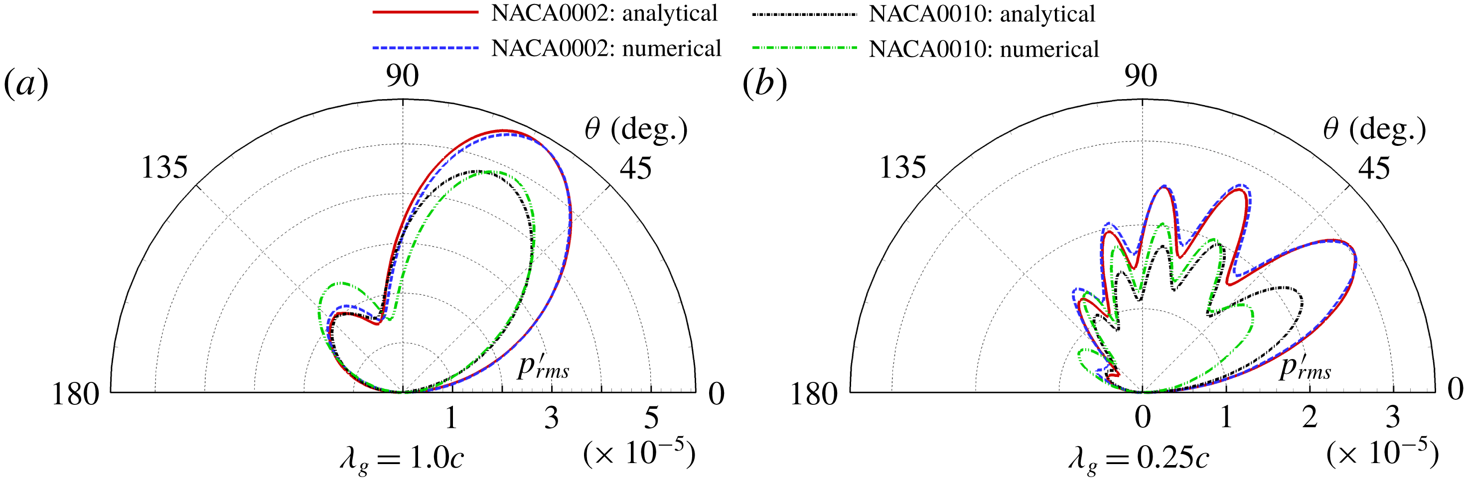
Figure 11. Analytical predictions of far-field $p_{rms}^{\prime }$ of airfoils interacting with gusts $\unicode[STIX]{x1D706}_{g}=1.0c$ and $0.25c$ at $M_{\infty }=0.5$ .

3.5 Applications to different gust wavelengths

In the previous section, it was shown that the proposed analytical correction method could improve the accuracy when compared with the numerical results for the cases with gust wavelength $\unicode[STIX]{x1D706}_{g}=0.5c$ . In this section, the performance of the prediction method is studied for alternative gusts with $\unicode[STIX]{x1D706}_{g}=0.25c$ and $\unicode[STIX]{x1D706}_{g}=1.0c$ . We focus on the NACA0002 and NACA0010 airfoils at Mach number $M_{\infty }=0.5$ , with angle of attack $\unicode[STIX]{x1D6FC}=0^{\circ }$ . Figure 11 shows the predicted far-field directivities in different configurations. In general, the predictions of the NACA0002 airfoil case match well with the numerical results. The sound reductions by the NACA0010 airfoil are captured for both gust wavelengths. However, in the upstream direction, the numerical results have larger values while the amplitudes of the radiation lobes are relatively smaller. For the higher-frequency case $\unicode[STIX]{x1D706}_{g}=0.25c$ , the analytical prediction underestimates the sound reduction in the downstream direction while it overestimates the reduction at moderate to high observer angles, i.e. $\unicode[STIX]{x1D703}>60^{\circ }$ . The disagreements are expected, as we have omitted some terms in the governing equations that could introduce approximation errors. As shown in appendix A, the order of the error of the term $\unicode[STIX]{x2202}/\unicode[STIX]{x2202}T$ is $O(M_{\infty })$ , suggesting that the prediction could be less accurate along with the increase of the frequency. This might be the reason why there are more noticeable differences in $p_{rms}^{\prime }$ of the NACA0010 airfoil with the numerical result in the upstream direction for the $\unicode[STIX]{x1D706}_{g}=0.25c$ case. Nevertheless, much improvement is obtained compared with the flat-plate solutions. Particularly for the cases in which the NACA0010 airfoil interacts with $\unicode[STIX]{x1D706}_{g}=1.0c$ and $0.25c$ gusts, the values of $I_{r}$ are 0.2659 and 0.5264, respectively.

3.6 Applications to oblique gusts ( $k_{2}\neq 0$ )

In the cases studied above, the gusts contain only the transverse disturbances ( $k_{2}=0$ ). However, streamwise disturbances may also be present, since a harmonic gust is a Fourier component of the turbulent fluctuations. In this section, the sound radiation using an oblique gust that contains both streamwise and transverse fluctuations is studied. The vortical gust is also in the 2-D domain, and the wavenumber in the transverse direction $k_{2}\neq 0$ . Typically, the gust wavelength is $\unicode[STIX]{x1D706}_{g}=0.5c$ and the incident angle is $\unicode[STIX]{x1D703}_{g}=45^{\circ }$ , i.e. the wavenumbers in both directions are $k_{1}=k_{2}=\sqrt{2}\unicode[STIX]{x03C0}/\unicode[STIX]{x1D706}_{g}$ . The Mach number is $0.5$ , and the NACA0002 and NACA0010 airfoils are studied for comparison.

Figure 12. Analytical prediction of far-field $p_{rms}^{\prime }$ of airfoils interacting with oblique gusts; here $M_{\infty }=0.5$ , $\unicode[STIX]{x1D706}_{g}=0.5c$ and $\unicode[STIX]{x1D703}_{g}=45^{\circ }$ .

Figure 12 shows the comparison of the predicted and numerical results for the oblique gusts. For the NACA0002 case, the predictions match reasonably well and are close to the flat-plate solution. In this case, the predicted results are equivalent to a different harmonic gust that contains only the transverse disturbance ( $k_{1}\rightarrow k_{1}/\sqrt{2}$ , $A_{v}\rightarrow A_{v}/\sqrt{2}$ ). By contrast, the prediction of the NACA0010 airfoil by the proposed method performs badly in capturing the radiation patterns, especially on the suction side. Figure 13 shows the pressure fields by the numerical simulation using the CAA solver. For the thin airfoil NACA0002, the sound field is nearly antisymmetric on the pressure and suction sides, while a significant difference exists for the NACA0010 airfoil. In the upstream direction, the value of the sound pressure has a non-zero value, suggesting that the condition $\unicode[STIX]{x1D719}=0$ for $x_{1}<0$ is invalid. Also, the streamwise disturbance interacting with the non-uniform mean flow may also lead to additional sound. These factors make the prediction by the analytical correction less valid for the thicker airfoils being subjected to oblique gusts. In this case, $I_{r}=1.08$ for the NACA0010 airfoil, which means that the proposed analytical correction does not produce a prediction superior to the classical flat-plate solution. To have a more accurate prediction while avoiding the drawbacks of the proposed correction in this work, one may use the methods based on the RDT by Goldstein (Reference Goldstein1978) or Atassi & Grzedzinski (Reference Atassi and Grzedzinski1989). In that case, the computation should be conducted in the 2-D domain if those more theoretically rigorous models are used.

Figure 13. Numerical computation of $p^{\prime }$ of airfoils interacting with oblique gusts (incident angle $45^{\circ }$ , shown in the inset) at $M_{\infty }=0.5$ .

3.7 Applications to broadband cases

In this work, we also investigate the acoustic broadband properties when the airfoils interact with the incoming turbulence. In the context of this work, the turbulence consists of gusts with different wavenumbers. For simplicity, the distribution of the amplitude of each wavenumber component is described by an isotropic Gaussian energy spectrum (Kraichnan Reference Kraichnan1970)

(3.2) $$\begin{eqnarray}E(k)=\frac{2}{\unicode[STIX]{x03C0}^{2}}u_{rms}^{\prime \,2}\unicode[STIX]{x1D6EC}^{4}k^{3}\exp \left(-\frac{\unicode[STIX]{x1D6EC}^{2}k^{2}}{\unicode[STIX]{x03C0}}\right),\end{eqnarray}$$

where $\unicode[STIX]{x1D6EC}$ is the integral length scale, $u_{rms}^{\prime }$ is the root-mean-square value of the turbulence kinetic velocity and $k=|\boldsymbol{k}|=\sqrt{k_{1}^{2}+k_{2}^{2}}$ is the wavenumber. The velocity spectra $\unicode[STIX]{x1D6F7}_{ij}(k_{1},k_{2})$ are calculated as (Gea-Aguilera et al. Reference Gea-Aguilera, Gill and Zhang2017)

(3.3) $$\begin{eqnarray}\unicode[STIX]{x1D6F7}_{ij}(k_{1},k_{2})=\frac{E(k)}{\unicode[STIX]{x03C0}k}\left(\unicode[STIX]{x1D6FF}_{ij}-\frac{k_{i}k_{j}}{k^{2}}\right)\quad \Rightarrow \quad \unicode[STIX]{x1D6F7}_{22}(k_{1},k_{2})=\frac{2}{\unicode[STIX]{x03C0}^{3}}u_{rms}^{\prime \,2}\unicode[STIX]{x1D6EC}^{4}k_{1}^{2}\exp \left(-\frac{\unicode[STIX]{x1D6EC}^{2}k^{2}}{\unicode[STIX]{x03C0}}\right).\end{eqnarray}$$

The amplitude of the gust component with wavenumber $(k_{1},k_{2})$ is computed as $A_{v}(k_{1},k_{2})=\sqrt{\unicode[STIX]{x1D6F7}_{22}(k_{1},k_{2})/k_{1}^{2}}$ using the divergence-free property of the gust. In this work, we set the dimensionless value $u_{rms}^{\prime }=0.01$ and $\unicode[STIX]{x1D6EC}=0.1c$ . For comparison, numerical simulations using the high-order CAA method are also conducted. In the CAA computation, the turbulent fluctuations are reproduced using an advanced synthetic turbulence method based on the digital filter approach (Gea-Aguilera et al. Reference Gea-Aguilera, Gill and Zhang2017).

Figure 14 shows the sound pressure distributions of the NACA0002 and NACA0012 airfoils determined by the CAA simulations. The integral length scale of the turbulence is $\unicode[STIX]{x1D6EC}=0.1c$ and the flow Mach number is $M_{\infty }=0.5$ . For the NACA0012 airfoil, the sound radiation is reduced in the downstream direction, while a stronger sound distribution is observed in the upstream direction. Figure 15 shows the far-field $p_{rms}^{\prime }$ of different airfoils predicted by the proposed method and by the numerical simulation. The simulation result of the NACA0002 airfoil is close to the flat-plate solution and the analytical solution. More sound reduction can be found in the downstream direction with the increase of airfoil thickness. There are apparent differences between the analytical and numerical simulation results for the real airfoils. However, the deviations are smaller than the differences between the numerical simulation and the flat-plate results. In the upstream direction, the predictions by the analytical solution are low and are close to the flat-plate solution, since we have assumed $\unicode[STIX]{x1D719}=0$ in the upstream direction ( $x_{1}<0$ ). By contrast, higher levels of sound to the upstream direction are found in the numerical simulations. In recent work by Zhong et al. (Reference Zhong, Zhang, Gill, Fattah and Sun2018) and Zhong & Zhang (Reference Zhong and Zhang2019), it is shown that the streamwise disturbance interacting with the near-field non-uniform mean flow can also contribute to sound generation in the upstream direction, which is not considered in this work. The errors are expected since reasonable approximations are made in the analytical correction, which, nevertheless, improves the prediction accuracy over the flat-plate solution.

Figure 14. Numerical computation of $p^{\prime }$ of airfoils interacting with an isotropic turbulence with $\unicode[STIX]{x1D6EC}=0.1c$ at $M_{\infty }=0.5$ .

Figure 15. Comparisons of far-field $p_{rms}^{\prime }$ obtained by the proposed correction and the numerical simulation, with $\unicode[STIX]{x1D6EC}=0.1c$ and $M_{\infty }=0.5$ .

At a lower Mach number $M_{\infty }=0.2$ , comparisons of far-field directivities of different airfoils are shown in figure 16. For the NACA0002 and NACA0006 airfoils, sound reduction due to the thickness is predicted and the analytical correction matches reasonably well with the numerical result. For airfoils with larger thickness, the difference in $p_{rms}^{\prime }$ between the analytical solution and the numerical results becomes discernible, especially at observer angles of approximately $60^{\circ }{-}70^{\circ }$ . However, the errors are much smaller than those at $M_{\infty }=0.5$ , being consistent with the error analysis in appendix A. The error in the upstream direction is not important at this speed. The variations of $I_{r}$ with airfoil thickness are shown in figure 17, in which the improvements by the proposed method are quantitatively measured.

Figure 16. Comparisons of far-field $p_{rms}^{\prime }$ obtained by the proposed correction and the numerical simulation, with $\unicode[STIX]{x1D6EC}=0.1c$ and $M_{\infty }=0.2$ .

Figure 17. The variation of $I_{r}$ with the increase of airfoil thickness for the broadband cases at $M_{\infty }=0.2$ and 0.5.

In this work, we also apply the proposed method to compute the acoustic responses for isotropic turbulences with Liepmann spectra (Gea-Aguilera et al. Reference Gea-Aguilera, Gill, Zhang, Chen and Nodé-Langlois2016):

(3.4a,b ) $$\begin{eqnarray}\unicode[STIX]{x1D6F7}_{11}(k_{1},k_{2})=\frac{2\unicode[STIX]{x1D6EC}^{5}u_{rms}^{\prime 2}k_{2}^{2}}{\unicode[STIX]{x03C0}^{2}(1+\unicode[STIX]{x1D6EC}^{2}k^{2})^{3}},\quad \unicode[STIX]{x1D6F7}_{22}(k_{1},k_{2})=\frac{2\unicode[STIX]{x1D6EC}^{5}u_{rms}^{\prime 2}k_{1}^{2}}{\unicode[STIX]{x03C0}^{2}(1+\unicode[STIX]{x1D6EC}^{2}k^{2})^{3}}.\end{eqnarray}$$

The turbulence integral length scale $\unicode[STIX]{x1D6EC}=0.053$ is studied for the NACA0012 airfoil at $M_{\infty }=0.3$ and 0.5. The numerical simulation is conducted using a new synthetic turbulence method (Shen & Zhang Reference Shen and Zhang2018). The comparisons of the flat-plate solution by Amiet (Reference Amiet1975), the numerical simulation and the analytical correction method proposed in this work are shown in figure 18. For the $M_{\infty }=0.3$ case, the result of the proposed analytical solution matches fairly well with the numerical result, and the sound reduction compared with the flat-plate solution is captured. For the $M_{\infty }=0.5$ case, the sound reduction due to the airfoil thickness is captured in the downstream direction. In the upstream direction, the results by the flat-plate solution and the proposed correction method are close, and are lower than that by the CAA computation, being similar to the Gaussian simulation results shown in figure 15.

Figure 18. Comparisons of far-field $p_{rms}^{\prime }$ for the NACA0012 airfoil obtained by the proposed correction and the numerical simulation. The turbulence has an isotropic Liepmann spectra and the integral length scale is $\unicode[STIX]{x1D6EC}=0.053c$ .

As for the time expense, in general, the numerical simulation takes approximately 12 h to obtain a steady mean flow, and takes another 12 h to simulate the acoustic response and to compute the far-field directivities (with ${\sim}$ 1.5 million grid points and ${\sim}$ 2 million simulation steps using 48 Intel Xeon E5-2670 processors). However, the time expense varies from case to case. For example, smaller grids are used in the NACA0002 airfoil to capture the sharp variation of the curvature at the leading edge, doubling the computational time. In the proposed solution, the calculation of a single-frequency case can be finished within 15 s, which is close to the implementation of Amiet’s solution for flat plates; while the total computation time for a typical broadband case is approximately 15–20 min (with four Intel i7-4790 processors). The number for wavenumber discretisation is tested to be sufficient in this work.