2. Nonlinear transformation of Navier–Stokes equations

This study originated from an issue faced by the authors while trying to use the forcing data from an LES database constructed using a primitive-like variable set (Towne Reference Towne2016; Brès et al. Reference Bres, Ham, Nichols and Lele2017, Reference Bres, Jordan, Jaunet, Le Rallic, Cavalieri, Towne, Lele, Colonius and Schmidt2018), with a resolvent analysis tool written in conservative variables (Bugeat et al. Reference Bugeat, Chassaing, Robinet and Sagaut2019). The problem can be illustrated by considering the effect of a nonlinear transformation of variables on the Navier–Stokes equations (though the analysis in fact applies to any nonlinear dynamical system).

2.1. Derivation

The Navier–Stokes equations (NSE) are written

(2.1)\begin{equation} \partial_t \boldsymbol{q} = \mathcal{N}(\boldsymbol{q}), \end{equation}

where $\boldsymbol {q}\in \mathbb {R}^m$ is the vector of state variables with $m=5$ for three-dimensional flows and $\mathcal {N}:\mathbb {R}^m\to \mathbb {R}^m$ is the nonlinear Navier–Stokes operator. Performing a Taylor-series expansion of $\boldsymbol {q}$ about a linearisation point $\bar {\boldsymbol {q}}$ in state space, which is typically the mean of $\boldsymbol {q}$, (2.1) can be written as

(2.2)\begin{equation} \partial_t \boldsymbol{q}^\prime -\mathcal{A}(\boldsymbol{q}^\prime) = \boldsymbol{f}, \end{equation}

where $(\cdot )^\prime$ denotes fluctuations, $\mathcal {A}\triangleq \textrm {D}\mathcal {N}(\bar {\boldsymbol {q}})$ is the Fréchet derivative of $\mathcal {N}$ at $\bar {\boldsymbol {q}}$ (which becomes the Jacobian $\boldsymbol{\mathsf{A}}\triangleq \partial _{q}\mathcal {N}|_{\bar {\boldsymbol {q}}}$ for the discretised NSE) and $\boldsymbol {f}$ denotes all the remaining nonlinear terms, i.e. $\boldsymbol {f}=\mathcal {N}(\boldsymbol {q})-\mathcal {A}(\boldsymbol {q}^\prime )$. Here, an analogy with the theory of linear time-invariant (LTI) systems can be made by considering $\boldsymbol{\mathsf{A}}$ as the system matrix and $\boldsymbol {q}^\prime$ as the response of this system to a forcing, $\boldsymbol {f}$. Resolvent analysis adopts this analogy to determine a forcing function $\boldsymbol {f}$ that maximises the linear gain associated with the resolvent operator, $\boldsymbol{\mathsf{R}}\triangleq (\textrm {i} \omega \boldsymbol{\mathsf{I}} - \boldsymbol{\mathsf{A}})^{-1}$.

To investigate the impact of the choice of variables, we define a nonlinear bijective transformation, $\mathcal {H}:\mathbb {R}^m\to \mathbb {R}^m$, as

(2.3)\begin{equation} \boldsymbol{q}_T \triangleq \mathcal{H}(\boldsymbol{q}), \end{equation}

which maps the state variable from the original to a new set of variables, e.g. from primitive to conservative variables. The governing equation (2.1) can be represented in terms of the transformed variable $\boldsymbol {q}_T$ by defining another operator, $\mathcal {N}_T$, that satisfies

(2.4)\begin{equation} \partial_t \boldsymbol{q}_T = \mathcal{N}_T(\boldsymbol{q}_T), \end{equation}

which can also be linearised around its mean, $\bar {\boldsymbol {q}}_T$, yielding

(2.5)\begin{equation} \partial_t \boldsymbol{q}_T^\prime -\mathcal{A}_T(\boldsymbol{q}_T^\prime) = \boldsymbol{f}_T. \end{equation}

In what follows, we express $\textrm {D}\mathcal {N}_T(\boldsymbol {q}_T)$ in terms of $\textrm {D}\mathcal {N}(\boldsymbol {q})$. Differentiating (2.3) with respect to time and inserting (2.1) and (2.4) in the result gives

(2.6)\begin{equation} \mathcal{N}_T(\boldsymbol{q}_T) =\textrm{D}\mathcal{H}(\boldsymbol{q})\mathcal{N}(\boldsymbol{q}), \end{equation}

where the multiplication with a Fréchet derivative defines an inner product. To calculate the Jacobian, we need to take the derivative of the left-hand side (LHS) of (2.6) with respect to $\boldsymbol {q}_T$, which is equivalent to taking the derivative of the right-hand side (RHS) with respect to $\mathcal {H}(\boldsymbol {q})$. Given that $\textrm {D} F(\mathcal {H}(\boldsymbol {q}))=\textrm {D}(F\circ \mathcal {H})(\boldsymbol {q})(\textrm {D} \mathcal {H}(\boldsymbol {q}) )^{-1}$ for a smooth $F$, the Jacobian can be written as

(2.7)\begin{equation} \textrm{D}\mathcal{N}_T(\boldsymbol{q}_T)= \textrm{D}\mathcal{H}(\boldsymbol{q})\textrm{D}\mathcal{N}(\boldsymbol{q}) (\textrm{D} \mathcal{H}(\boldsymbol{q}) )^{{-}1} + \textrm{D}^2\mathcal{H}(\boldsymbol{q}) (\textrm{D} \mathcal{H}(\boldsymbol{q}) )^{{-}1}\mathcal{N}(\boldsymbol{q}). \end{equation}

The LHS of (2.7) should be calculated at $\bar {\boldsymbol {q}}_T$ in order to obtain $\mathcal {A}_T$. The state vectors $\bar {\boldsymbol {q}}$ and $\bar {\boldsymbol {q}}_T$ are not equivalent in the sense that they do not satisfy (2.3), i.e. $\bar {\boldsymbol {q}}_T\neq \mathcal {H}(\bar {\boldsymbol {q}})$. The equivalent expansion point for the RHS of (2.7), which is not equal to $\bar {\boldsymbol {q}}$, is then defined as

(2.8)\begin{equation} \tilde{\boldsymbol{q}}\triangleq\mathcal{H}^{{-}1}(\bar{\boldsymbol{q}}_T). \end{equation}

Calculation of $\bar {\boldsymbol {q}}_T$ requires the dynamic state data. In case only the mean flow statistics are available, a first-order prediction of $\tilde {\boldsymbol {q}}$ can be achieved as described in appendix A.

Having defined $\tilde {\boldsymbol {q}}$, (2.7) can then be rewritten as

(2.9)\begin{equation} {\mathcal{A}}_{T}= \textrm{D}\mathcal{H}(\tilde{\boldsymbol{q}})\tilde{\mathcal{A}} (\textrm{D} \mathcal{H}(\tilde{\boldsymbol{q}}) )^{{-}1} + \textrm{D}^2\mathcal{H}(\tilde{\boldsymbol{q}}) (\textrm{D} \mathcal{H}(\tilde{\boldsymbol{q}}) )^{{-}1} \mathcal{N}(\tilde{\boldsymbol{q}}), \end{equation}

where $\tilde {\mathcal {A}}\triangleq \textrm {D}\mathcal {N}(\tilde {\boldsymbol {q}})$. Note that the second term on the RHS of (2.7) is zero if $\mathcal {H}$ is linear ($\textrm {D}^2\mathcal {H}(\boldsymbol {q})=0$ for any $\boldsymbol {q}$) or if linearisation is performed about a ‘fixed’ point of the system, which, by definition, satisfies $\mathcal {N}(\bar {\boldsymbol {q}})=0$. In that case, the first term in (2.9) indicates a similarity transformation between ${\mathcal {A}}_T$ and $\tilde {\mathcal {A}}$, which now reduces to $\mathcal {A}$ (due to having $\bar {\boldsymbol {q}}_T= \mathcal {H}(\bar {\boldsymbol {q}})$ satisfied, by definition in the case of linear $\mathcal {H}$, and through (2.6) in the case of expansion around the fixed point), and the two linear operators share the same eigenvalues. In mean-flow-based linear analysis, however, the second term on the RHS of (2.9) is non-zero, which implies a difference in the eigenvalues of $\tilde {\mathcal {A}}$ and ${\mathcal {A}}_T$ even if the corresponding linearisation points are equivalent.

We now derive an expression relating $\mathcal {A}$ and $\mathcal {A}_T$. It is more convenient to compare these two operators since one would use $\mathcal {A}$ rather than $\tilde {\mathcal {A}}$ when performing mean-flow linear analysis. Although (2.9) provides a means to compute $\mathcal {A}_T$, which can then be compared to $\mathcal {A}$, an exact general expression relating the two operators cannot be derived for nonlinear $\mathcal {H}$. However, an approximate relation is given by replacing (A 5) into (2.9) as

(2.10)\begin{align} {\mathcal{A}}_{T} & \approx \textrm{D}\mathcal{H}(\tilde{\boldsymbol{q}}){\mathcal{A}} (\textrm{D}\mathcal{H}(\tilde{\boldsymbol{q}}) )^{{-}1} + \textrm{D}\mathcal{H}(\tilde{\boldsymbol{q}}) (\mathcal{A}\textrm{D}\epsilon(\bar{\boldsymbol{q}}) + \textrm{D}^2\mathcal{N}(\bar{\boldsymbol{q}})\epsilon(\bar{\boldsymbol{q}}) ) (\textrm{D}\mathcal{H}(\tilde{\boldsymbol{q}}) )^{{-}1} \nonumber\\ & \quad + \textrm{D}^2\mathcal{H}(\tilde{\boldsymbol{q}}) (\textrm{D}\mathcal{H}(\tilde{\boldsymbol{q}}) )^{{-}1}\mathcal{N}(\tilde{\boldsymbol{q}}). \end{align}

The second term on the RHS of (2.10) accounts for the change in the linearisation point, i.e. non-equivalence of the mean flows, $\bar {\boldsymbol {q}}$ and $\bar {\boldsymbol {q}}_T$, due to taking the mean after nonlinear transformation, while the third term appears once again since the mean flow is not a fixed point of the Navier–Stokes system for turbulent flows. It is obvious that these extra terms do not cancel each other for arbitrary $\mathcal {H}$. As a result, expanded about the mean flow, the system characteristics are modified when subjected to a nonlinear transformation. An immediate implication is that the stability characteristics of the linear operator are not unique and the linearised systems (2.2) and (2.5) are equivalent only if the right-hand sides are maintained and the equal sign is respected.

2.2. Implications for resolvent analysis

Resolvent analysis involves taking the Fourier transform of (2.2), or similarly (2.5), and reorganising the result as

(2.11)\begin{equation} \hat{\boldsymbol{q}}= \boldsymbol{\mathsf{R}}\hat{\boldsymbol{f}}, \end{equation}

where $\hat {\boldsymbol {q}}$ and $\hat {\boldsymbol {f}}$ are the Fourier transforms of $\boldsymbol {q}$ and $\boldsymbol {f}$, respectively. Ignoring the nonlinear relation between $\hat {\boldsymbol {f}}$ and $\hat {\boldsymbol {q}}$, (2.11) can be seen as a forcing–response relation. The optimal forcing that would maximise the energy in the response can be found by maximising the Rayleigh quotient, $\sigma \triangleq {\langle \hat {\boldsymbol {q}}, \hat {\boldsymbol {q}} \rangle }/{\langle \,\hat {\boldsymbol {f}}, \hat {\boldsymbol {f}}\rangle }$, where the inner product is defined as

(2.12)\begin{equation} \langle \boldsymbol{a},\boldsymbol{b} \rangle = \int_V \boldsymbol{a}^* \boldsymbol{\mathsf{M}}\boldsymbol{b}\,\textrm{d}V, \end{equation}

with $\boldsymbol{\mathsf{M}}$ defining a suitable energy norm. The Rayleigh quotient for the transformed system, $\sigma _T$, can be similarly defined using $\hat {\boldsymbol {q}}_T$ and $\hat {\boldsymbol {f}}_T$. To compare $\sigma$ and $\sigma _T$, the energy norms in the original and the transformed systems should be equivalent, which amounts to

(2.13)\begin{equation} \int_V {\boldsymbol{q}^\prime}^* \boldsymbol{\mathsf{M}}\boldsymbol{q}^\prime\,\textrm{d}V =\int_V {\boldsymbol{q}^\prime}^*_T \boldsymbol{\mathsf{M}}_T\boldsymbol{q}^\prime_T \,\textrm{d}V. \end{equation}

To leading order in fluctuation amplitude, $\boldsymbol {q}^\prime _T$ and $\boldsymbol {q}^\prime$ are related by the expression

(2.14)\begin{equation} \boldsymbol{q}^\prime_T=\partial_q\mathcal{H}|_{\bar{q}}\,\boldsymbol{q}^\prime. \end{equation}

Replacing $\boldsymbol {q}^\prime _T$ terms in (2.13) using (2.14) yields a leading-order norm equivalence:

(2.15)\begin{equation} \boldsymbol{\mathsf{M}}=\partial_q\mathcal{H}|_{\bar{q}}^* \,\boldsymbol{\mathsf{M}}_T\partial_q \mathcal{H}|_{\bar{q}}. \end{equation}

Note that the norm correction is required even when the variable transformation is linear, in which case the resolvent operators are connected through a similarity transform. Equation (2.15) can alternatively be obtained by enforcing that the Rayleigh quotients of the original and linearly transformed systems be equal.

3. Application to test cases

The above analysis is tested using four different LES databases of ideally expanded round jets: three isothermal jets at $M_j=0.4$, 0.9 and 1.5, and a hot jet at $M_j=1.5$ are investigated to observe the effect of switching from conservative to primitive variable sets on resolvent analysis (table 1). The operating conditions are given in terms of jet exit Mach number, $M_j$, nozzle pressure ratio, $NPR\triangleq P_{0,j}/P_\infty$, nozzle temperature ratio, $NTR\triangleq T_{0,j}/T_\infty$, and Reynolds number, $Re\triangleq \rho _jU_jD/\mu _j$, where $D$ is the nozzle diameter, $\mu _j$ is the dynamic viscosity at the jet exit, and the subscript 0 is used to denote stagnation quantities. Further details about the LES databases can be found in Brès et al. (Reference Bres, Ham, Nichols and Lele2017, Reference Bres, Jordan, Jaunet, Le Rallic, Cavalieri, Towne, Lele, Colonius and Schmidt2018).

Table 1. The list of axisymmetric jets investigated.

For each flow case, we performed resolvent analysis and spectral proper orthogonal decomposition (SPOD) of the axisymmetric mode using two different variable sets: $[\nu \ u_x\ u_r\ p]^\textrm {T}$ and $[\rho \ \rho u_x\ \rho u_r\ \rho E]^\textrm {T}$, which we refer to as primitive and conservative, respectively. Here, $\nu =1/\rho$, $\rho$, $u_x$, $u_r$, $p$ and $\rho E$ denote the specific volume, density, axial and radial velocities, pressure and total energy, respectively. In order to perform a singular value decomposition (SVD) of the resolvent, the Jacobian matrix of the compressible NSE, i.e. the linear operator $\boldsymbol{\mathsf{A}}$ defined in § 2.1, is computed using conservative variables by linearising the discretised equation as described by Mettot et al. (Reference Mettot, Renac and Sipp2014). At this point, it is possible to switch to primitive variables by first finding the linearisation point that is equivalent to the mean in primitive variables using (2.8), and then applying (2.9) to get $\boldsymbol{\mathsf{A}}_T$. The SVD of the resolvent is then calculated based on Krylov methods as detailed in Bugeat et al. (Reference Bugeat, Chassaing, Robinet and Sagaut2019). The open libraries PETSc (Balay et al. Reference Balay, Gropp, McInnes and Smith1997) and SLEPc (Hernandez et al. Reference Hernandez, Roman and Vidal2005) are used to solve the linear systems by direct LU decomposition and eigenvalue calculation by the Krylov–Schur algorithm (Hernández et al. Reference Hernández, Román, Tomás and Vidal2007). Computations are carried out using an orthogonal mesh of $748\times 229$ points for the subsonic cases, and $636\times 229$ points for the supersonic cases, which were determined after a convergence study, in the numerical domain $x/D \in [0;30]$ and $r/D \in [0;12]$, where $x/D=0$ is the location of the nozzle exit and $r/D=0$ is the centreline. Sponge zones are located at $x/D>20$ and $r/D>5$. The Chu norm (Chu Reference Chu1965) is used for both response and forcing over $x/D \in [0;20]$ and $r/D \in [0;5]$.

To calculate the SPOD modes, we followed the method introduced by Towne et al. (Reference Towne, Schmidt and Colonius2018). Once again, the Chu norm is used. We calculated the fast Fourier transform (FFT) of $\boldsymbol {q}$ with 128 FFT points, and overlap ratio of 0.75, yielding 310 FFT blocks for the isothermal cases, and 154 blocks for the hot jet case.

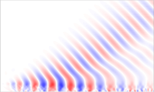
The optimum response modes at $St=0.6$ obtained using primitive and conservative variables, respectively, are plotted in comparison to the optimum SPOD modes in primitive variables in figure 1 for all jet cases. Figure 1 shows the pressure field, which is directly computed for the primitive-variable cases, while it is reconstructed using (2.14) for the conservative-variable cases. The reconstructed SPOD modes are identical to the directly computed ones (see table 4), so are not shown here. The mode shapes are very similar between the directly computed and the reconstructed response modes. However, the global weight distribution among the variables slightly differs in Jet-4 (higher for pressure in the reconstructed mode).

Figure 1. Comparison of the leading SPOD (left) and optimal resolvent (centre, right) modes at $St=0.6$ for different jets: (a) Jet-1 to (d) Jet-4, respectively. Pressure fields are shown. For the analyses using conservative variables (right), pressure is obtained through linearised transformation.

The transformation from primitive to conservative variables, which are denoted by the subscripts $p$ and $c$, respectively, is defined as $\boldsymbol {q}_c=\mathcal {H}(\boldsymbol {q}_p),$ with

(3.1)\begin{equation} \mathcal{H}(\boldsymbol{q})=\left[\frac{1}{\boldsymbol{q}_1},\ \frac{\boldsymbol{q}_2}{\boldsymbol{q}_1},\ \frac{\boldsymbol{q}_3}{\boldsymbol{q}_1},\frac{\boldsymbol{q}_4}{(\gamma-1)}+\frac{1}{2}\frac{1}{\boldsymbol{q}_1} (\boldsymbol{q}_2^2+\boldsymbol{q}_3^2 )\right]^\textrm{T}, \end{equation}

where $\gamma =1.4$ is the heat capacity ratio. This function becomes linear for density and momentum terms when the flow is incompressible. The jet cases are listed in the order of increasing variable-density effects. Therefore we expect larger deviation in the singular values of the original and transformed resolvent operators as we move from Jet-1 to Jet-4. To quantify the effect of density fluctuations on the mean flow, we define the percentage measure ${\rm \Delta} \bar {\boldsymbol {q}} \triangleq [|\mathcal {H}^{-1}(\bar {\boldsymbol {q}}_c) - \bar {\boldsymbol {q}}_p| / \bar {\boldsymbol {q}}_p] \times 100$. We integrate this quantity over the jet domain where turbulent kinetic energy is greater than 1 % of its maximum value and normalise the result with the integration domain. To quantify the change in the singular values, we define ${\rm \Delta} \sigma _1 \triangleq [(\sigma _{1,c}-\sigma _{1,p}) / \sigma _{1,p}] \times 100$ and ${\rm \Delta} G \triangleq [(G_c-G_p) / G_p] \times 100$, where $G=\sigma _1/\sigma _2$ is the gain separation between the optimal and the first suboptimal singular values. The modification of the mean and the resulting changes in the singular values are tabulated in table 2. It can be seen from the table that the difference between the true mean, $\bar {\boldsymbol {q}}_p$, and the transformed mean, $\mathcal {H}^{-1}(\bar {\boldsymbol {q}}_c)$, does not exceed 0.6 % except in the radial velocity field, where 7.6 % overall difference is seen in Jet-4. The radial profiles of the mean flow calculated directly in primitive variables, $\bar {\boldsymbol {q}}_p$, and reconstructed from conservative variables, $\tilde {\boldsymbol {q}}_p$, are shown for Jet-4 in figure 2. Once again, the difference between $\bar {\boldsymbol {q}}_p$ and $\tilde {\boldsymbol {q}}_p$ is mostly visible in radial velocity and pressure around the shear layer, with the largest percentage change in the former. This difference indicates a relatively strong correlation between density and radial velocity, and similarly between density and pressure, in this region. Despite the small modification of the mean, the optimal singular value and gain separation are modified by up to 40 % and 35 %, respectively, in Jet-4.

Figure 2. Radial mean flow profiles calculated in primitive variables (solid) and reconstructed from conservative variables (dashed) at $x/D=2$ in Jet-4.

Table 2. The change in the mean fields and the singular values calculated at $St=0.6$ due to transformation from primitive to conservative variables.

For the two supersonic cases, Jet-3 and Jet-4, in which noticeable changes in the singular values are observed, the analysis is repeated at different frequencies. The optimal gain spectra obtained using primitive variables and their modification under variable transformation are plotted in figure 3. It is seen that the maximum change in singular values is obtained at $St=0.4$ and $St=0.6$ for Jet-3 and Jet-4, respectively.

Figure 3. Optimal gain spectra computed using primitive variables (a), and their modification under variable transformation (b).

We furthermore investigate the alignment of the optimum response mode of the resolvent operator with the leading SPOD mode of the response, $\boldsymbol {q}$. The alignment is quantified as the absolute value of the scalar product, $|\langle \boldsymbol {\psi }_S,\boldsymbol {\psi }_R\rangle |$, where the subscripts $R$ and $S$ stand for the resolvent optimal response and SPOD modes, respectively. The results at $St=0.6$ are tabulated in table 3 for all jets. It is seen that the alignment is slightly better when primitive variables are used, except for Jet-4, where the alignment is improved by $\sim$24 % when conservative variables are used, although the gain separation is lowered by 35 %. This is counter-intuitive since the alignment of SPOD and resolvent modes is often associated with high gain separation in the resolvent operator (Beneddine et al. Reference Beneddine, Sipp, Arnault, Dandois and Lesshafft2016), considering that the nonlinear terms are close to white noise and thus have similar projection coefficients onto the forcing mode basis. However, the presence of coherent low-rank forcing, as recently observed for turbulent channel flow (Morra et al. Reference Morra, Nogueira, Cavalieri and Henningson2020), may change this picture. The overall weight of a response mode in $\hat {\boldsymbol {q}}$ is determined by the corresponding gain together with the projection of the actual forcing, $\hat {\boldsymbol {f}}$ on to the corresponding forcing mode of the resolvent operator. Therefore, the observed increase in the alignment despite the reduction in gain separation indicates enhanced projection of forcing onto the optimal forcing mode, which is sufficient to outweigh the reduced gain separation.

Table 3. Alignment coefficients between the leading SPOD and response modes for different jet cases at $St=0.6$. Results obtained using primitive and conservative variables, respectively, are compared.

Table 4. Alignment coefficients between the directly computed and the reconstructed modes for different jet cases at $St=0.6$.

Finally, we investigate the change in SPOD and resolvent modes that occurs under the variable transformation. We transform the modes obtained using conservative variables to their primitive-variable counterparts using (2.14). The inner-product definition given in (2.12) is now used to measure the alignment between the reconstructed and directly calculated modes. The results at $St=0.6$ are tabulated in table 4. The alignment of the leading SPOD modes calculated in conservative and primitive variables is above 98 % for all the jets. The similarity of directly computed and reconstructed optimal resolvent modes are again above 98 % for all the cases except for the heated compressible Jet-4, where we see a drop to 46 %. This change, consistent with the significant change observed in the singular values, shows how the choice of variables may lead to quite different results and subsequent conclusions about the underlying flow physics.