


1. Introduction
The behaviour of liquid–solid–gas contact lines, at which an ambient gas is displaced by a liquid spreading over a solid, is the key element of many technological processes, ranging from coating flows used to apply thin liquid films to substrates (Weinstein & Ruschak Reference Weinstein and Ruschak2004) to 3D printers being developed to economically produce bespoke geometrically complex structures (Derby Reference Derby2010). Often, limitations on the operating devices are imposed by ‘wetting failure’, which occurs when the liquid can no longer completely displace the gas at the contact line. In coating technologies, this leads to the entrainment of gas bubbles into the liquid film, which destroy its carefully tuned material properties, while in drop-based flows entrainment of air under the moving contact line promotes the formation of splashes, which, again, are usually undesirable. Consequently, an understanding of the physical mechanisms that control wetting failure and, where possible, delay of this occurrence by manipulating the material parameters, flow geometry, etc. to ever increasing wetting speeds are some of the key aims of research into dynamic wetting.
Recent experimental studies have discovered new ways in which to delay the onset of wetting failures. Specifically, in both coating flows (Benkreira & Khan Reference Benkreira and Khan2008; Benkreira & Ikin Reference Benkreira and Ikin2010) and drop impact phenomena (Xu, Zhang & Nagel Reference Xu, Zhang and Nagel2005; Xu Reference Xu2007) it has been shown that a sufficient reduction in the pressure of the ambient gas, by approximately a factor of ten in the former case and even less in the latter, can suppress wetting failures. This result was unexpected, as until the work of Xu et al. (Reference Xu, Zhang and Nagel2005) it was assumed that the gas dynamics can either be entirely neglected or, as found in coating research, only influences the system behaviour through viscous forces that act in the thin gas film in front of the moving contact line (Kistler Reference Kistler and Berg1993). However, the significance of the viscous forces in the gas is usually characterised by the viscosity ratio between the gas and the liquid, and this remains unchanged by variations in gas pressure. Why then, would reductions in ambient pressure have any influence on the contact line dynamics?
An interpretation of the aforementioned phenomena, suggested in a number of different contexts, is that the reduction in ambient gas pressure, which leads to a corresponding decrease in gas density, increases the mean free path in this phase so that non-equilibrium gas dynamics (Chapman & Cowling Reference Chapman and Cowling1970), also referred to as rarefied gas dynamics (Cercignani Reference Cercignani2000), become important (Benkreira & Ikin Reference Benkreira and Ikin2010; Duchemin & Josserand Reference Duchemin and Josserand2012; Marchand et al. Reference Marchand, Chan, Snoeijer and Andreotti2012). Specifically, boundary slip is generated in the gas, whose magnitude is proportional to the mean free path and thus whose influence is increased by reductions in gas pressure. The increased slip allows gas trapped in thin films between the solid and the free surface to escape more easily, so that the lubrication forces generated by the gas are reduced and its influence is negated.
For drop impact phenomena, the literature of which has been previously reviewed (Rein Reference Rein1993; Yarin Reference Yarin2006), alterations in the lubrication forces could be important either (a) in the thin air cushion that exists under the drop before it impacts the solid (Thoroddsen, Etoh & Takehara Reference Thoroddsen, Etoh and Takehara2005; Bouwhuis et al. Reference Bouwhuis, van der Veen, Tran, Keij, Winkels, Peters, van der Meer, Sun, Snoeijer and Lohse2012) and/or (b) in the gas film formed in front of the advancing contact line after the drop has impacted the solid (Riboux & Gordillo Reference Riboux and Gordillo2014), see figure 1. Theoretical work has also focused on either (a) the pre-impact stage (Smith, Li & Wu Reference Smith, Li and Wu2003; Mani, Mandre & Brenner Reference Mani, Mandre and Brenner2010; Mandre & Brenner Reference Mandre and Brenner2012) or (b) the post-impact spreading phase where, with a few exceptions (Schroll et al. Reference Schroll, Josserand, Zaleski and Zhang2010), the gas is usually considered to be passive (Bussmann, Chandra & Mostaghimi Reference Bussmann, Chandra and Mostaghimi2000; Eggers et al. Reference Eggers, Fontelos, Josserand and Zaleski2010; Sprittles & Shikhmurzaev Reference Sprittles and Shikhmurzaev2012a ). It is a complex problem to distinguish how each of these processes influences the spreading dynamics of the drop, from both a theoretical and an experimental perspective, due to the inherently multiscale nature of the phenomenon. As a result, it remains an area of intensive debate to establish how reductions in ambient pressure suppress splashing (Driscoll & Nagel Reference Driscoll and Nagel2011; Kolinski et al. Reference Kolinski, Rubinstein, Mandre, Brenner, Weitz and Mahadevan2012; de Ruiter et al. Reference de Ruiter, Oh, Ende and Mugele2012), with recent experimental results on the impact stage being particularly interesting (Kolinski, Mahadevan & Rubinstein Reference Kolinski, Mahadevan and Rubinstein2014; de Ruiter et al. Reference de Ruiter, Lagraauw, Ende and Mugele2015; Liu, Tan & Xu Reference Liu, Tan and Xu2015).

Figure 1. Sketch illustrating the influence of gas flow on the drop impact phenomenon. The behaviour of the gas, in the regions indicated by black arrows, affects both (a) the pre-impact and (b) the post-impact spreading dynamics of the drop.
In contrast to drop-based dynamics, for the dip-coating flow investigated in Benkreira & Khan (Reference Benkreira and Khan2008) mechanism (a) does not exist, as up until the point of wetting failure, the liquid remains in contact with the solid and the motion is steady. Therefore, study of this process allows us to isolate the influence of changes in ambient pressure on the behaviour of a moving contact line, i.e. effect (b), without any of the aforementioned complications that are inherent to the drop impact phenomenon. This is the path that will be pursued in the present work, with drop dynamics only reconsidered again in § 7 where, having characterised fully (b), our results enable us to infer some conclusions about drop splashing phenomena.
1.1. Experimental observations in dip coating
The experimental set-up constructed in Benkreira & Khan (Reference Benkreira and Khan2008) is for dip coating, where a plate/tape is continuously run through a liquid bath (figure 2) and gradually increased in speed until air is entrained into the liquid. The speed at which this first occurs is called the ‘maximum speed of wetting’ and will be denoted by
 $U_{c}^{\star }$
, where stars will be used throughout to denote dimensional quantities. In contrast to previous works (Burley & Kennedy Reference Burley and Kennedy1976; Blake & Shikhmurzaev Reference Blake and Shikhmurzaev2002), the ambient gas pressure
$U_{c}^{\star }$
, where stars will be used throughout to denote dimensional quantities. In contrast to previous works (Burley & Kennedy Reference Burley and Kennedy1976; Blake & Shikhmurzaev Reference Blake and Shikhmurzaev2002), the ambient gas pressure
 $P_{g}^{\star }$
can be reduced from its atmospheric value by up to a factor of a hundred by mounting this apparatus inside a vacuum chamber. Silicone oils of differing viscosities are used as the coating liquid, because their relatively low volatility (compared with, say, water–glycerol mixtures) ensures no significant evaporation when the ambient pressure is reduced. This work is extended in Benkreira & Ikin (Reference Benkreira and Ikin2010) to consider also a range of different ambient gases (air, carbon dioxide and helium). The key results from Benkreira & Khan (Reference Benkreira and Khan2008) can be summarised as follows.
$P_{g}^{\star }$
can be reduced from its atmospheric value by up to a factor of a hundred by mounting this apparatus inside a vacuum chamber. Silicone oils of differing viscosities are used as the coating liquid, because their relatively low volatility (compared with, say, water–glycerol mixtures) ensures no significant evaporation when the ambient pressure is reduced. This work is extended in Benkreira & Ikin (Reference Benkreira and Ikin2010) to consider also a range of different ambient gases (air, carbon dioxide and helium). The key results from Benkreira & Khan (Reference Benkreira and Khan2008) can be summarised as follows.
-
(a) For a given liquid–solid–gas system,
 $U_{c}^{\star }$
can be increased by reducing
$P_{g}^{\star }$
.
$U_{c}^{\star }$
can be increased by reducing
$P_{g}^{\star }$
. -
(b) There is very little variation in
$U_{c}^{\star }$
until
$P_{g}^{\star }$
is approximately a tenth of its atmospheric value. Further reductions in
$P_{g}^{\star }$
lead to sharp increases in
$U_{c}^{\star }$
. -
(c) For sufficiently low
$P_{g}^{\star }$
, it is possible for high-viscosity liquids to have a larger value of
$U_{c}^{\star }$
than lower-viscosity ones (the opposite of what occurs at atmospheric pressure).


Figure 2. Sketch of the dip-coating flow configuration, showing a free surface formed between a liquid (below) and gas (above), with density and viscosity
 ${\it\rho},{\it\mu}$
and
${\it\rho},{\it\mu}$
and
 ${\it\rho}_{g},{\it\mu}_{g}$
, respectively. The free surface meets a solid surface at a contact line, which is a distance
${\it\rho}_{g},{\it\mu}_{g}$
, respectively. The free surface meets a solid surface at a contact line, which is a distance
 ${\rm\Delta}y$
below the height of the surface (
${\rm\Delta}y$
below the height of the surface (
 $y=0$
). The unit vectors normal to the free-surface and solid are, respectively,
$y=0$
). The unit vectors normal to the free-surface and solid are, respectively,
 $\boldsymbol{n}$
and
$\boldsymbol{n}$
and
 $\boldsymbol{n}_{s}$
. The inset shows that the free surface meets the solid at a contact angle
$\boldsymbol{n}_{s}$
. The inset shows that the free surface meets the solid at a contact angle
 ${\it\theta}_{d}$
but that a finite distance away has an apparent angle
${\it\theta}_{d}$
but that a finite distance away has an apparent angle
 ${\it\theta}_{M}$
at an inflection point in the surface profile where the film has height
${\it\theta}_{M}$
at an inflection point in the surface profile where the film has height
 $H$
.
$H$
.
In addition to these findings, in Benkreira & Ikin (Reference Benkreira and Ikin2010) the following is shown.
-
(d) For a given value of
$P_{g}^{\star }$
, use of a gas with a larger mean free path increases
$U_{c}^{\star }$
.


In Benkreira & Ikin (Reference Benkreira and Ikin2010), the aforementioned experimental observations are assumed to be caused by non-equilibrium effects in the gas which become significant at sufficiently low pressures. These effects, most notably slip at the boundaries of the gas film, are interpreted in terms of an ‘effective gas viscosity’ whose magnitude is reduced with decreases in ambient gas pressure. Use of appropriate values for this parameter, obtained from measurements of the resistance of a gas trapped between parallel oscillating plates (Andrews & Harris Reference Andrews and Harris1995), allows the data to be collapsed onto a single curve (figure 9b in Benkreira & Ikin Reference Benkreira and Ikin2010) and highlights the influence of non-equilibrium effects.
Although the effective viscosity may be a useful concept when trying to qualitatively interpret the experimental findings, as an integral property of the system it will not enable us to formulate a local fluid mechanical model for this problem. In particular, the dependence of the effective gas viscosity on the ambient gas pressure which is used in Benkreira & Ikin (Reference Benkreira and Ikin2010) was obtained in Andrews & Harris (Reference Andrews and Harris1995) for a gas film of constant height
 $2~{\rm\mu}\text{m}$
and will be different for other film profiles. In reality, the gas film height will vary all the way from the contact line to the far field, where a film can no longer be defined so that the notion of an effective viscosity no longer makes sense. Instead, we must look to capture the local physical mechanisms that alter the gas film dynamics at reduced pressures.
$2~{\rm\mu}\text{m}$
and will be different for other film profiles. In reality, the gas film height will vary all the way from the contact line to the far field, where a film can no longer be defined so that the notion of an effective viscosity no longer makes sense. Instead, we must look to capture the local physical mechanisms that alter the gas film dynamics at reduced pressures.
1.2. Mathematical modelling of dynamic wetting phenomena
We consider the various levels of description that can be used to describe dynamic wetting phenomena depending on how the gas dynamics are accounted for, with the simplest case first.
1.2.1. Dynamic wetting in a passive gas
In many cases, the viscosity and density ratios indicate that the gas can be treated as dynamically passive. Then, mathematical models for the liquid dynamics must address two key aspects. First, the classical fluid mechanical model, with no-slip at fluid–solid boundaries, has no solution (Huh & Scriven Reference Huh and Scriven1971; Shikhmurzaev Reference Shikhmurzaev2006). This is the so-called ‘moving contact-line problem’. Second, the contact angle, which is seen to vary at experimental resolutions (Hoffman Reference Hoffman1975; Blake & Shikhmurzaev Reference Blake and Shikhmurzaev2002), must be prescribed as a boundary condition on the free-surface shape. A review of the various classes of models proposed to address these issues can be found in chap. 3 of Shikhmurzaev (Reference Shikhmurzaev2007).
To overcome the moving contact-line problem, initially identified in Huh & Scriven (Reference Huh and Scriven1971), it is often assumed that some degree of slip occurs at the fluid–solid boundary (Dussan V Reference Dussan1976). Methods for predicting the ‘slip length’ of an arbitrary liquid–solid interface are not well developed, but estimates suggest that it is in the range 1–10 nm for simple liquids (Lauga, Brenner & Stone Reference Lauga, Brenner and Stone2007).
The treatment of the dynamic contact angle remains a highly contentious issue. The main question is whether or not the experimentally observed variation in the ‘apparent angle’ (Wilson et al. Reference Wilson, Summers, Shikhmurzaev, Clarke and Blake2006) is caused entirely by the bending of the free surface below the resolution of the experiment, i.e. by the ‘viscous bending’ mechanism quantified in Cox (Reference Cox1986) and measured in Dussan V, Ramé & Garoff (Reference Dussan, Ramé and Garoff1991) and Ramé & Garoff (Reference Ramé and Garoff1996), or whether the actual contact angle (sometimes referred to as the ‘microscopic angle’) also varies. In either case, the apparent angle depends on the capillary number, which is the dimensionless contact-line speed, but in the former case the actual angle remains fixed while in the latter this angle varies, as in the molecular kinetic theory (Blake & Haynes Reference Blake and Haynes1969). In more complex models, the angle can also depend on the flow field itself, as in the interface formation model (Shikhmurzaev Reference Shikhmurzaev2007).
Models in which the contact angle is considered to be constant have been popular in recent years for investigating air entrainment phenomena and have produced a number of promising results (Marchand et al. Reference Marchand, Chan, Snoeijer and Andreotti2012; Vandre, Carvalho & Kumar Reference Vandre, Carvalho and Kumar2012, Reference Vandre, Carvalho and Kumar2013, Reference Vandre, Carvalho and Kumar2014; Chan et al. Reference Chan, Srivastava, Marchand, Andreotti, Biferale, Toschi and Snoeijer2013). What is clear from simulations is that viscous bending of the free surface becomes significant as the point of air entrainment is approached, and cannot be neglected. What remains unclear is whether this mechanism is sufficient to account for the experimentally observed dynamics of the apparent contact angle, particularly given that precise measurements of the magnitude of slip on the liquid–solid interface are lacking. These difficulties have stimulated fundamental research into the contact-line region dynamics using molecular dynamics techniques (De Coninck & Blake Reference De Coninck and Blake2008), but, as can be seen from a recent collection of papers (Velarde Reference Velarde and Velarde2011) and review articles (Blake Reference Blake2006; Snoeijer & Andreotti Reference Snoeijer and Andreotti2013), intense debate remains about the topic.
The focus of this work is to characterise the effects that the gas dynamics can have on dynamic wetting phenomena, and, consequently, the simplest possible model for the other aspects will be used. Specifically, slip at the liquid–solid interface will be captured using the Navier condition (Navier Reference Navier1823), as commonly used in dynamic wetting models (Hocking Reference Hocking1976; Huh & Mason Reference Huh and Mason1977), and the contact angle will be taken as a parameter that is fixed at its equilibrium value. The result is a ‘conventional model’, and a comprehensive review of all such models that can be ‘built’ is given in chap. 9 of Shikhmurzaev (Reference Shikhmurzaev1997). More complex models can easily be constructed on top of the model used here, but in the present context would distract from the main focus of this work.
1.2.2. In a viscous gas
It is now well recognised that at sufficiently high coating speeds a thin film of gas forms in front of the moving contact line, as observed experimentally by laser-Doppler velocimetry in Mues, Hens & Boiy (Reference Mues, Hens and Boiy1989). The thin nature of the film means that despite the large viscosity ratio, lubrication forces enhance the influence of the gas dynamics so that they cannot be neglected. As coating speeds are increased, the resistance this film creates to contact-line motion eventually becomes sufficiently large that it is entrained into the liquid (Marchand et al. Reference Marchand, Chan, Snoeijer and Andreotti2012; Vandre et al. Reference Vandre, Carvalho and Kumar2013). Therefore, to study the phenomenon of air entrainment and wetting failures, any theory developed must account for the dynamics of the viscous gas as well as the liquid.
In formulating a model for the gas dynamics one again encounters the moving contact-line problem, namely that if no-slip is used then the contact line cannot move. Consequently, slip has also often been applied on the solid–gas boundary with a magnitude, measured by the slip length, either explicitly stated to be the same as in the liquid (Vandre et al. Reference Vandre, Carvalho and Kumar2013) or implicitly assumed to be so (Cox Reference Cox1986). In other words, slip is usually used as a mathematical fix to circumvent the moving contact-line problem, rather than as a physical effect whose magnitude can significantly alter the flow.
1.2.3. In a non-equilibrium gas
Experimental observations in Marchand et al. (Reference Marchand, Chan, Snoeijer and Andreotti2012), where the gas film entrained by a plunging plate was measured using optical methods, suggest that for relatively viscous liquids the characteristic film thickness is rather small, in the range
 $H^{\star }\sim 1{-}15~{\rm\mu}\text{m}$
. For flows where there is an external load on the film, such as in curtain coating, the film thickness is likely to be even smaller. Consequently, the film dimensions become comparable with the mean free path in the gas
$H^{\star }\sim 1{-}15~{\rm\mu}\text{m}$
. For flows where there is an external load on the film, such as in curtain coating, the film thickness is likely to be even smaller. Consequently, the film dimensions become comparable with the mean free path in the gas
 $\ell ^{\star }$
, so that the Knudsen number
$\ell ^{\star }$
, so that the Knudsen number
 $\mathit{Kn}_{H}=\ell ^{\star }/H^{\star }$
, characterising the importance of non-equilibrium gas effects, becomes non-negligible, particularly at reduced pressures. For example, a factor of 10 decrease in the ambient pressure of air, achieved in both Xu et al. (Reference Xu, Zhang and Nagel2005) and Benkreira & Khan (Reference Benkreira and Khan2008), gives a value of
$\mathit{Kn}_{H}=\ell ^{\star }/H^{\star }$
, characterising the importance of non-equilibrium gas effects, becomes non-negligible, particularly at reduced pressures. For example, a factor of 10 decrease in the ambient pressure of air, achieved in both Xu et al. (Reference Xu, Zhang and Nagel2005) and Benkreira & Khan (Reference Benkreira and Khan2008), gives a value of
 $\ell ^{\star }=0.7~{\rm\mu}\text{m}$
, so that
$\ell ^{\star }=0.7~{\rm\mu}\text{m}$
, so that
 $\mathit{Kn}_{H}\sim 0.1$
. In this case, one may expect that non-equilibrium effects in the gas film will have a significant impact on its dynamics, and we must consider how this can be incorporated into our dynamic wetting model.
$\mathit{Kn}_{H}\sim 0.1$
. In this case, one may expect that non-equilibrium effects in the gas film will have a significant impact on its dynamics, and we must consider how this can be incorporated into our dynamic wetting model.
Non-equilibrium effects first manifest themselves at the boundaries of the gas and can be accounted for by relaxing the no-slip condition to allow for boundary slip while continuing to use the Navier–Stokes equations in the bulk. This approach remains accurate for
 $\mathit{Kn}_{H}<0.1$
, during which gas flow is said to be in the ‘slip regime’, after which Knudsen layers will begin to occupy the entire gas film, so that the scale separation between boundary and bulk effects no longer exists.
$\mathit{Kn}_{H}<0.1$
, during which gas flow is said to be in the ‘slip regime’, after which Knudsen layers will begin to occupy the entire gas film, so that the scale separation between boundary and bulk effects no longer exists.
In Maxwell (Reference Maxwell1879), a slip condition was derived for the ‘micro-slip’ at the actual boundary of the gas, whose mathematical form remains the same, when
 $\mathit{Kn}_{H}\ll 1$
, if ‘macro-slip’ across a Knudsen layer of size
$\mathit{Kn}_{H}\ll 1$
, if ‘macro-slip’ across a Knudsen layer of size
 ${\sim}\ell ^{\star }$
is also accounted for, see § 3.5 of Cercignani (Reference Cercignani2000). We shall henceforth refer to the discontinuity in tangential velocity as ‘Maxwell slip’, which at an impermeable boundary is generated by the shear stress acting on that interface from the gas phase. For two-dimensional isothermal flow, the component of velocity
${\sim}\ell ^{\star }$
is also accounted for, see § 3.5 of Cercignani (Reference Cercignani2000). We shall henceforth refer to the discontinuity in tangential velocity as ‘Maxwell slip’, which at an impermeable boundary is generated by the shear stress acting on that interface from the gas phase. For two-dimensional isothermal flow, the component of velocity
 $u_{g}^{\star }$
, where subscript
$u_{g}^{\star }$
, where subscript
 $g$
will denote properties of the gas, adjacent to a stationary planar surface located at
$g$
will denote properties of the gas, adjacent to a stationary planar surface located at
 $y=0$
is, in dimensional terms, given by
$y=0$
is, in dimensional terms, given by
 $$\begin{eqnarray}a\,\ell ^{\star }\,\frac{\partial u_{g}^{\star }}{\partial y^{\star }}=u_{g}^{\star },\end{eqnarray}$$
where the coefficient of proportionality
 $a$
can depend on both the properties of the micro-slip, which will depend on the fraction of molecules that reflect diffusively and those that are purely specular, and the macro-slip generated across a Knudsen layer. In practice, unless surfaces are molecularly smooth we will have
$a$
can depend on both the properties of the micro-slip, which will depend on the fraction of molecules that reflect diffusively and those that are purely specular, and the macro-slip generated across a Knudsen layer. In practice, unless surfaces are molecularly smooth we will have
 $a\sim 1$
(Millikan Reference Millikan1923; Allen & Raabe Reference Allen and Raabe1982; Agarwal & Prabhu Reference Agarwal and Prabhu2008) and, for simplicity, we will henceforth take
$a\sim 1$
(Millikan Reference Millikan1923; Allen & Raabe Reference Allen and Raabe1982; Agarwal & Prabhu Reference Agarwal and Prabhu2008) and, for simplicity, we will henceforth take
 $a=1$
.
$a=1$
.
The Maxwell-slip condition (1.1) has the same form as the slip conditions that have often been used in dynamic wetting flows to circumvent the moving contact-line problem in the gas, but occurs naturally here from the consideration of non-equilibrium effects. Notably, this means that accurate values of the slip length can easily be obtained by knowing the mean free path in the gas, in contrast to the slip length in the liquid which is notoriously difficult to determine. Furthermore, the approach taken here suggests that slip will also be present at the gas–liquid boundary (i.e. the free surface), as demonstrated by experiments dating back to Millikan (Reference Millikan1923). This effect is shown in figure 3, where the parameter
 $A$
is used to change between the usual condition of continuity of velocity across the gas–liquid interface (
$A$
is used to change between the usual condition of continuity of velocity across the gas–liquid interface (
 $A=0$
) and Maxwell slip (
$A=0$
) and Maxwell slip (
 $A=1$
).
$A=1$
).

Figure 3. The effect of Maxwell slip on the gas flow. When (a)
 $A=0$
slip is present at the gas–solid boundary but turned off at the gas–liquid boundary, so that
$A=0$
slip is present at the gas–solid boundary but turned off at the gas–liquid boundary, so that
 $\boldsymbol{u}_{g}=\boldsymbol{u}$
, while (b) for
$\boldsymbol{u}_{g}=\boldsymbol{u}$
, while (b) for
 $A=1$
it is present on both interfaces.
$A=1$
it is present on both interfaces.
Slip at the gas–liquid boundary has been accounted for in some models for the gas film in drop impact (Mani et al. Reference Mani, Mandre and Brenner2010; Duchemin & Josserand Reference Duchemin and Josserand2012), and in great detail for drop collisions (Sundararajakumar & Koch Reference Sundararajakumar and Koch1996), but is yet to be routinely incorporated into dynamic wetting models. In most cases where slip on the gas–solid interface is accounted for, the same effect on the gas–liquid surface is not considered (Vandre et al. Reference Vandre, Carvalho and Kumar2013; Riboux & Gordillo Reference Riboux and Gordillo2014). The only progress in this direction has been achieved in Marchand et al. (Reference Marchand, Chan, Snoeijer and Andreotti2012), where non-equilibrium effects are accounted for by modifying the viscosity in the gas. However, this is achieved by using an empirical expression for the effective viscosity which suffers from the same issues as mentioned previously, namely a reliance on the lubrication approximation that does not enable one to fully formulate a uniformly valid local fluid mechanical problem.
In order to apply Maxwell slip at curved moving surfaces, the tensorial expression is required (Lockerby et al.
Reference Lockerby, Reese, Emerson and Barber2004). Specifically, for gas flow adjacent to a surface that moves with velocity
 $\boldsymbol{u}^{\star }$
and has normal
$\boldsymbol{u}^{\star }$
and has normal
 $\boldsymbol{n}$
pointing into the gas, we have
$\boldsymbol{n}$
pointing into the gas, we have
 $$\begin{eqnarray}\ell ^{\star }\,\boldsymbol{n}\boldsymbol{\cdot }(\boldsymbol{{\rm\nabla}}\boldsymbol{u}_{g}^{\star }+[\boldsymbol{{\rm\nabla}}\boldsymbol{u}_{g}^{\star }]^{\text{T}})\boldsymbol{\cdot }(\unicode[STIX]{x1D644}-\boldsymbol{n}\boldsymbol{n})=\boldsymbol{u}_{g\Vert }^{\star }-\boldsymbol{u}_{\Vert }^{\star },\end{eqnarray}$$
where the subscript
 $\Vert$
denotes the components of a vector tangential to the surface, which can be obtained for an arbitrary vector
$\Vert$
denotes the components of a vector tangential to the surface, which can be obtained for an arbitrary vector
 $\boldsymbol{a}$
using
$\boldsymbol{a}$
using
 $\boldsymbol{a}_{\Vert }=\boldsymbol{a}\boldsymbol{\cdot }\left(\unicode[STIX]{x1D644}-\boldsymbol{n}\boldsymbol{n}\right)$
, where
$\boldsymbol{a}_{\Vert }=\boldsymbol{a}\boldsymbol{\cdot }\left(\unicode[STIX]{x1D644}-\boldsymbol{n}\boldsymbol{n}\right)$
, where
 $\unicode[STIX]{x1D644}$
is the metric tensor of the coordinate system.
$\unicode[STIX]{x1D644}$
is the metric tensor of the coordinate system.
If the gas is modelled as being composed of ‘hard spheres’, then the mean free path is related to the temperature
 $T^{\star }$
and ambient pressure
$T^{\star }$
and ambient pressure
 $P_{g}^{\star }$
by
$P_{g}^{\star }$
by
 $\ell ^{\star }=k_{B}^{\star }T^{\star }/(\sqrt{2}{\rm\pi}P_{g}^{\star }(l_{mol}^{\star })^{2})$
, where
$\ell ^{\star }=k_{B}^{\star }T^{\star }/(\sqrt{2}{\rm\pi}P_{g}^{\star }(l_{mol}^{\star })^{2})$
, where
 $l_{mol}^{\star }$
is the molecular diameter and
$l_{mol}^{\star }$
is the molecular diameter and
 $k_{B}^{\star }$
is Boltzmann’s constant. Notably, if local variations in gas pressure about
$k_{B}^{\star }$
is Boltzmann’s constant. Notably, if local variations in gas pressure about
 $P_{g}^{\star }$
are small, as confirmed in § 4.5, then for a given ambient pressure
$P_{g}^{\star }$
are small, as confirmed in § 4.5, then for a given ambient pressure
 $\ell ^{\star }$
is approximately constant throughout the entire gas phase. In practice, when considering the dependence of the mean free path of a gas on the ambient pressure at a fixed temperature it is convenient to use the expression
$\ell ^{\star }$
is approximately constant throughout the entire gas phase. In practice, when considering the dependence of the mean free path of a gas on the ambient pressure at a fixed temperature it is convenient to use the expression
 $$\begin{eqnarray}\bar{\ell }\equiv \frac{\ell ^{\star }}{\ell _{atm}^{\star }}=\frac{P_{g,atm}^{\star }}{P_{g}^{\star }}\equiv 1/\bar{P}_{g},\end{eqnarray}$$
where
 $\bar{P}_{g}$
is the gas pressure normalised by its atmospheric value. At atmospheric pressure, air has a mean free path
$\bar{P}_{g}$
is the gas pressure normalised by its atmospheric value. At atmospheric pressure, air has a mean free path
 $\ell _{atm}^{\star }=0.07~{\rm\mu}\text{m}$
and other commonly encountered gases take similar values
$\ell _{atm}^{\star }=0.07~{\rm\mu}\text{m}$
and other commonly encountered gases take similar values
 $\ell _{atm}^{\star }\sim 0.1~{\rm\mu}\text{m}$
.
$\ell _{atm}^{\star }\sim 0.1~{\rm\mu}\text{m}$
.
Although the Knudsen number in the gas film
 $\mathit{Kn}_{H}$
is of most interest, this can only be obtained once our computations have allowed us to find
$\mathit{Kn}_{H}$
is of most interest, this can only be obtained once our computations have allowed us to find
 $H^{\star }$
. Before then, the Knudsen number based on our characteristic scale
$H^{\star }$
. Before then, the Knudsen number based on our characteristic scale
 $\mathit{Kn}=\ell ^{\star }/L^{\star }$
, where
$\mathit{Kn}=\ell ^{\star }/L^{\star }$
, where
 $L^{\star }\sim 1~\text{mm}$
is the capillary length, must be used. Noting that the dimensionless mean free path at atmospheric pressure is
$L^{\star }\sim 1~\text{mm}$
is the capillary length, must be used. Noting that the dimensionless mean free path at atmospheric pressure is
 $\ell _{atm}=\ell _{atm}^{\star }/L^{\star }$
, the resulting expression for
$\ell _{atm}=\ell _{atm}^{\star }/L^{\star }$
, the resulting expression for
 $\mathit{Kn}$
takes the form
$\mathit{Kn}$
takes the form
 $$\begin{eqnarray}\mathit{Kn}=\frac{\ell _{atm}}{\bar{P}_{g}},\end{eqnarray}$$
so that the explicit dependence on pressure reduction becomes clear.
1.3. Overview
This work will answer the following questions.
-
(a) Can increases in Maxwell slip, caused by experimentally attainable reductions in ambient gas pressure, significantly raise the maximum speed of wetting?
-
(b) Does slip on the liquid–gas interface, usually neglected in this class of flows, have a substantial effect on the dynamic wetting process?
-
(c) Will the magnitude of the Knudsen number based on the gas film height
$\mathit{Kn}_{H}$
be small enough for the gas flow to remain in the ‘slip regime’? -
(d) Is it possible to collapse the data from Xu et al. (Reference Xu, Zhang and Nagel2005) onto a master curve by assuming that non-equilibrium gas effects are responsible for splash suppression in drop impact?

The paper is organised as follows. In § 2 the dip-coating problem will be formulated and dimensionless parameters will be identified. The mathematical model for this process will be seen to be inherently multiscale, with flow dynamics on the nano-, micro- and milli-metre scale caused by, respectively, slip in the liquid, slip in the gas and capillarity. The computation of such multiscale flows is challenging, and neglecting to resolve all scales in the problem yields inaccurate results (Sprittles & Shikhmurzaev Reference Sprittles and Shikhmurzaev2012c ). In § 3, the application of a computational framework developed in Sprittles & Shikhmurzaev (Reference Sprittles and Shikhmurzaev2012c , Reference Sprittles and Shikhmurzaev2013) to this problem is described, which resolves all scales, and our method for defining a maximum speed of wetting is shown. Benchmark computations performed at atmospheric pressure are provided in appendix A. In § 4 the effects of the non-equilibrium gas dynamics on a base state are analysed and the gas flow is described in a lubrication setting. Subsequently, in § 5, a parametric study of the new system is conducted which allows us to identify the importance of the various competing physical mechanisms in the experimentally verifiable regimes before, in § 6, directly comparing our computations with experimental data. The implications of these findings for the drop impact phenomenon are considered in § 7. Finally, in § 8, potential avenues of enquiry for future theoretical and experimental development in this area are highlighted.
2. Problem formulation
We consider the flow generated by the steady motion of a smooth chemically homogeneous solid surface which is driven through a liquid–gas free surface in a direction aligned with gravity at a constant speed
 $U^{\star }$
(see figure 2). A characteristic length scale for this problem is given by the capillary length
$U^{\star }$
(see figure 2). A characteristic length scale for this problem is given by the capillary length
 $L^{\star }=\sqrt{{\it\sigma}^{\star }/(({\it\rho}^{\star }-{\it\rho}_{g}^{\star })g^{\star })}\simeq \sqrt{{\it\sigma}^{\star }/({\it\rho}^{\star }g^{\star })}$
, where
$L^{\star }=\sqrt{{\it\sigma}^{\star }/(({\it\rho}^{\star }-{\it\rho}_{g}^{\star })g^{\star })}\simeq \sqrt{{\it\sigma}^{\star }/({\it\rho}^{\star }g^{\star })}$
, where
 ${\it\sigma}^{\star }$
is the surface tension of the liquid–gas surface, which is assumed to be constant,
${\it\sigma}^{\star }$
is the surface tension of the liquid–gas surface, which is assumed to be constant,
 $g^{\star }$
is the acceleration due to gravity and
$g^{\star }$
is the acceleration due to gravity and
 ${\it\rho}^{\star },{\it\rho}_{g}^{\star }$
are the densities in the liquid and gas respectively, with
${\it\rho}^{\star },{\it\rho}_{g}^{\star }$
are the densities in the liquid and gas respectively, with
 ${\it\rho}_{g}^{\star }/{\it\rho}^{\star }\ll 1$
in the liquid–gas systems of interest, so that the capillary length can be determined solely from the liquid density. The scale for pressure is
${\it\rho}_{g}^{\star }/{\it\rho}^{\star }\ll 1$
in the liquid–gas systems of interest, so that the capillary length can be determined solely from the liquid density. The scale for pressure is
 ${\it\mu}^{\star }U^{\star }/L^{\star }$
, where
${\it\mu}^{\star }U^{\star }/L^{\star }$
, where
 ${\it\mu}^{\star }$
is the viscosity of the liquid and
${\it\mu}^{\star }$
is the viscosity of the liquid and
 ${\it\mu}_{g}^{\star }$
will be its value in the gas.
${\it\mu}_{g}^{\star }$
will be its value in the gas.
2.1. Bulk equations
For compressibility effects in the liquid and the gas to be negligible we require that the Mach number
 $\mathit{Ma}=U^{\star }/c^{\star }$
in each phase remains small, where
$\mathit{Ma}=U^{\star }/c^{\star }$
in each phase remains small, where
 $c^{\star }$
is the speed of sound. Given that
$c^{\star }$
is the speed of sound. Given that
 $U^{\star }<1~\text{m s}^{-1}$
and
$U^{\star }<1~\text{m s}^{-1}$
and
 $c^{\star }>100~\text{m s}^{-1}$
in all cases considered, we have
$c^{\star }>100~\text{m s}^{-1}$
in all cases considered, we have
 $\mathit{Ma}<0.01$
. However, this is not a sufficient condition for the flow to be considered incompressible, especially when there are thin films of gas present along which pressure can vary significantly, see § 4.5 of Gad-el-Hak (Reference Gad-el-Hak2006). Here, we will assume that the flow in both phases can be described by the steady incompressible Navier–Stokes equations, and in § 4.5 the validity of this assumption will be confirmed from a posteriori calculations. Therefore, we have
$\mathit{Ma}<0.01$
. However, this is not a sufficient condition for the flow to be considered incompressible, especially when there are thin films of gas present along which pressure can vary significantly, see § 4.5 of Gad-el-Hak (Reference Gad-el-Hak2006). Here, we will assume that the flow in both phases can be described by the steady incompressible Navier–Stokes equations, and in § 4.5 the validity of this assumption will be confirmed from a posteriori calculations. Therefore, we have
 $$\begin{eqnarray}\displaystyle \boldsymbol{{\rm\nabla}}\boldsymbol{\cdot }\boldsymbol{u}=0,\quad \mathit{Ca}\,\boldsymbol{u}\boldsymbol{\cdot }\boldsymbol{{\rm\nabla}}\boldsymbol{u}=\mathit{Oh}^{2}\left(\boldsymbol{{\rm\nabla}}\boldsymbol{\cdot }\boldsymbol{P}+\hat{\boldsymbol{g}}/\mathit{Ca}\right), & & \displaystyle\end{eqnarray}$$
 $$\begin{eqnarray}\displaystyle \boldsymbol{{\rm\nabla}}\boldsymbol{\cdot }\boldsymbol{u}_{g}=0,\quad \bar{{\it\rho}}\,\mathit{Ca}\,\boldsymbol{u}_{g}\boldsymbol{\cdot }\boldsymbol{{\rm\nabla}}\boldsymbol{u}_{g}=\mathit{Oh}^{2}\left(\boldsymbol{{\rm\nabla}}\boldsymbol{\cdot }\boldsymbol{P}_{g}+\bar{{\it\rho}}\,\hat{\boldsymbol{g}}/\mathit{Ca}\right), & & \displaystyle\end{eqnarray}$$
 $$\begin{eqnarray}\boldsymbol{P}=-p\unicode[STIX]{x1D644}+[\boldsymbol{{\rm\nabla}}\boldsymbol{u}+(\boldsymbol{{\rm\nabla}}\boldsymbol{u})^{\text{T}}]\quad \text{and}\quad \boldsymbol{P}_{g}=-p_{g}\unicode[STIX]{x1D644}+\bar{{\it\mu}}[\boldsymbol{{\rm\nabla}}\boldsymbol{u}_{g}+(\boldsymbol{{\rm\nabla}}\boldsymbol{u}_{g})^{\text{T}}].\end{eqnarray}$$
Here,
 $\boldsymbol{u}$
and
$\boldsymbol{u}$
and
 $\boldsymbol{u}_{g}$
are the velocities in the liquid and gas;
$\boldsymbol{u}_{g}$
are the velocities in the liquid and gas;
 $p$
and
$p$
and
 $p_{g}$
are the local pressures in the liquid and gas, in contrast to the uppercase
$p_{g}$
are the local pressures in the liquid and gas, in contrast to the uppercase
 $P$
that is used for the ambient pressure in the gas;
$P$
that is used for the ambient pressure in the gas;
 $\mathit{Ca}={\it\mu}^{\star }U^{\star }/{\it\sigma}^{\star }$
is the capillary number based on the viscosity of the liquid; the viscosity ratio is
$\mathit{Ca}={\it\mu}^{\star }U^{\star }/{\it\sigma}^{\star }$
is the capillary number based on the viscosity of the liquid; the viscosity ratio is
 $\bar{{\it\mu}}={\it\mu}_{g}^{\star }/{\it\mu}^{\star }$
; the ratio of gas to liquid densities is
$\bar{{\it\mu}}={\it\mu}_{g}^{\star }/{\it\mu}^{\star }$
; the ratio of gas to liquid densities is
 $\bar{{\it\rho}}={\it\rho}_{g}^{\star }/{\it\rho}^{\star }$
; and
$\bar{{\it\rho}}={\it\rho}_{g}^{\star }/{\it\rho}^{\star }$
; and
 $\hat{\boldsymbol{g}}$
is a unit vector aligned with the gravitational field. The Ohnesorge number
$\hat{\boldsymbol{g}}$
is a unit vector aligned with the gravitational field. The Ohnesorge number
 $\mathit{Oh}={\it\mu}^{\star }/\sqrt{{\it\rho}^{\star }{\it\sigma}^{\star }L^{\star }}$
has been chosen as a dimensionless parameter, instead of the Reynolds number
$\mathit{Oh}={\it\mu}^{\star }/\sqrt{{\it\rho}^{\star }{\it\sigma}^{\star }L^{\star }}$
has been chosen as a dimensionless parameter, instead of the Reynolds number
 $Re=\mathit{Ca}/\mathit{Oh}^{2}={\it\rho}^{\star }U^{\star }L^{\star }/{\it\mu}^{\star }$
, as for a given liquid–solid–gas combination
$Re=\mathit{Ca}/\mathit{Oh}^{2}={\it\rho}^{\star }U^{\star }L^{\star }/{\it\mu}^{\star }$
, as for a given liquid–solid–gas combination
 $\mathit{Oh}$
will remain constant, i.e. it will depend solely on material parameters and be independent of contact-line speed.
$\mathit{Oh}$
will remain constant, i.e. it will depend solely on material parameters and be independent of contact-line speed.
2.2. Boundary conditions at the gas–solid surface
Conditions of impermeability and Maxwell slip give
 $$\begin{eqnarray}\boldsymbol{u}_{g}\boldsymbol{\cdot }\boldsymbol{n}_{s}=0,\quad \mathit{Kn}\,\boldsymbol{n}_{s}\boldsymbol{\cdot }\boldsymbol{P}_{g}\boldsymbol{\cdot }\left(\unicode[STIX]{x1D644}-\boldsymbol{n}_{s}\boldsymbol{n}_{s}\right)=\boldsymbol{u}_{g\Vert }-\boldsymbol{U}_{\Vert },\end{eqnarray}$$
where
 $\boldsymbol{U}$
is the velocity of the solid and the normal to the solid surface is denoted as
$\boldsymbol{U}$
is the velocity of the solid and the normal to the solid surface is denoted as
 $\boldsymbol{n}_{s}$
.
$\boldsymbol{n}_{s}$
.
2.3. Boundary conditions at the liquid–gas free surface
On the free surface, whose location must be obtained as part of the solution, for a steady flow the kinematic equation and continuity of the normal component of velocity give that
 $$\begin{eqnarray}\boldsymbol{u}\boldsymbol{\cdot }\boldsymbol{n}=\boldsymbol{u}_{g}\boldsymbol{\cdot }\boldsymbol{n}=0,\end{eqnarray}$$
where
 $\boldsymbol{n}$
is the normal to the surface pointing into the liquid phase. These equations are combined with the standard balance of stresses with capillarity that give
$\boldsymbol{n}$
is the normal to the surface pointing into the liquid phase. These equations are combined with the standard balance of stresses with capillarity that give
 $$\begin{eqnarray}\boldsymbol{n}\boldsymbol{\cdot }(\boldsymbol{P}-\boldsymbol{P}_{g})\boldsymbol{\cdot }(\unicode[STIX]{x1D644}-\boldsymbol{n}\boldsymbol{n})=\mathbf{0},\quad \boldsymbol{n}\boldsymbol{\cdot }(\boldsymbol{P}-\boldsymbol{P}_{g})\boldsymbol{\cdot }\boldsymbol{n}=\boldsymbol{{\rm\nabla}}\boldsymbol{\cdot }\boldsymbol{n}/\mathit{Ca}.\end{eqnarray}$$
Equations (2.5) and (2.6) are usually combined with a condition stating that the velocity tangential to the interface is continuous across it,
 $\boldsymbol{u}_{g\Vert }=\boldsymbol{u}_{\Vert }$
. However, when Maxwell slip is accounted for this is replaced with
$\boldsymbol{u}_{g\Vert }=\boldsymbol{u}_{\Vert }$
. However, when Maxwell slip is accounted for this is replaced with
 $$\begin{eqnarray}-\!A\,\mathit{Kn}\,\boldsymbol{n}\boldsymbol{\cdot }\boldsymbol{P}_{g}\boldsymbol{\cdot }\left(\unicode[STIX]{x1D644}-\boldsymbol{n}\boldsymbol{n}\right)=\boldsymbol{u}_{g\Vert }-\boldsymbol{u}_{\Vert },\end{eqnarray}$$
where the minus sign occurs because the normal points into the liquid. By setting
 $A=0$
, Maxwell slip can be ‘turned off’ at the gas–liquid interface, see figure 3, as has been the case in previous dynamic wetting works which only consider slip at the solid boundary.
$A=0$
, Maxwell slip can be ‘turned off’ at the gas–liquid interface, see figure 3, as has been the case in previous dynamic wetting works which only consider slip at the solid boundary.
2.4. Boundary conditions at the liquid–solid surface
The standard conditions of impermeability and Navier slip give
 $$\begin{eqnarray}\boldsymbol{u}\boldsymbol{\cdot }\boldsymbol{n}_{s}=0,\quad l_{s}\,\boldsymbol{n}_{s}\boldsymbol{\cdot }\boldsymbol{P}\boldsymbol{\cdot }\left(\unicode[STIX]{x1D644}-\boldsymbol{n}_{s}\boldsymbol{n}_{s}\right)=\boldsymbol{u}_{\Vert }-\boldsymbol{U}_{\Vert },\end{eqnarray}$$
where
 $l_{s}=l_{s}^{\star }/L^{\star }$
is the dimensionless slip length based on the (dimensional) slip length at the liquid–solid interface
$l_{s}=l_{s}^{\star }/L^{\star }$
is the dimensionless slip length based on the (dimensional) slip length at the liquid–solid interface
 $l_{s}^{\star }$
. This parameter has no relation to the slip coefficient in the gas which was based on the mean free path
$l_{s}^{\star }$
. This parameter has no relation to the slip coefficient in the gas which was based on the mean free path
 $\ell ^{\star }$
. In other words, although Maxwell slip and Navier slip have the same mathematical form, their physical origins differ and thus there is no reason to expect their coefficients to have similar magnitudes.
$\ell ^{\star }$
. In other words, although Maxwell slip and Navier slip have the same mathematical form, their physical origins differ and thus there is no reason to expect their coefficients to have similar magnitudes.
2.5. Liquid–solid–gas contact line
Equation (2.6b
) requires a boundary condition at the contact line which is given by prescribing the contact angle
 ${\it\theta}_{d}$
satisfying
${\it\theta}_{d}$
satisfying
 $$\begin{eqnarray}\boldsymbol{n}\boldsymbol{\cdot }\boldsymbol{n}_{s}=-\!\cos {\it\theta}_{d}.\end{eqnarray}$$
Here, our focus is on understanding the effects of the gas dynamics on the dynamic wetting flow, so that we will take the simplest option of assuming
 ${\it\theta}_{d}$
to be a constant. More complex implementations, such as those in Sprittles & Shikhmurzaev (Reference Sprittles and Shikhmurzaev2013), can be considered in future research.
${\it\theta}_{d}$
to be a constant. More complex implementations, such as those in Sprittles & Shikhmurzaev (Reference Sprittles and Shikhmurzaev2013), can be considered in future research.
2.6. ‘Far-field’ conditions
Dip coating is usually conducted in a tank of finite size whose dimensions are large enough not to alter the dynamics close to the contact line, as confirmed in Benkreira & Khan (Reference Benkreira and Khan2008). The influence of system geometry, or ‘confinement’, on the dynamic wetting process is well known (Ngan & Dussan V Reference Ngan and Dussan1982), and, in particular, has been used to delay air entrainment (Vandre et al.
Reference Vandre, Carvalho and Kumar2012), but this effect is not the focus of the present work. Therefore, the ‘far-field’ boundaries of our domain, which are assumed to be no-slip solids,
 $\boldsymbol{u}=\boldsymbol{u}_{g}=\mathbf{0}$
, are set sufficiently far from the contact line that they have no influence on the dynamic wetting process. Where the free surface meets the far field it is assumed to be perpendicular to the gravitational field, i.e. ‘flat’, so that
$\boldsymbol{u}=\boldsymbol{u}_{g}=\mathbf{0}$
, are set sufficiently far from the contact line that they have no influence on the dynamic wetting process. Where the free surface meets the far field it is assumed to be perpendicular to the gravitational field, i.e. ‘flat’, so that
 $\boldsymbol{n}\boldsymbol{\cdot }\hat{\boldsymbol{g}}=1$
. In practice, setting the far field (dimensionally) to be twenty capillary lengths from the contact line was found to be sufficiently remote.
$\boldsymbol{n}\boldsymbol{\cdot }\hat{\boldsymbol{g}}=1$
. In practice, setting the far field (dimensionally) to be twenty capillary lengths from the contact line was found to be sufficiently remote.
3. Computational framework
Dynamic wetting and dewetting flows have often been investigated using the simplifications afforded by the lubrication approximation (Voinov Reference Voinov1976; Eggers Reference Eggers2004). However, for the two-phase flow considered here, this approximation cannot simultaneously be valid in each phase, i.e. the liquid and gas phases cannot both be thin films. As shown in recent papers (Marchand et al. Reference Marchand, Chan, Snoeijer and Andreotti2012; Vandre et al. Reference Vandre, Carvalho and Kumar2013), plausible extensions in the spirit of the lubrication approach can be attempted, but their accuracy can only be ascertained from comparisons with full computations and is unlikely to be acceptable at larger capillary numbers where the contact-line region cannot be considered as ‘localised’.
At present, to obtain accurate solutions to the mathematical model formulated in § 2, one is left with no option other than to use computational methods.
Computationally, resolution of all scales in the problem is particularly important to ensure that our contact line (2.9) is applied to the ‘actual’ or ‘microscopic’ angle
 ${\it\theta}_{d}$
, rather than the ‘apparent one’
${\it\theta}_{d}$
, rather than the ‘apparent one’
 ${\it\theta}_{app}={\it\theta}_{app}(s)$
, i.e. the angle of the free surface at a finite distance
${\it\theta}_{app}={\it\theta}_{app}(s)$
, i.e. the angle of the free surface at a finite distance
 $s$
from the contact line. Although the apparent angle can, in certain circumstances, be related to the actual angle (Cox Reference Cox1986), this will not be true at the high capillary numbers observed in coating flows, particularly when non-standard gas dynamics are included.
$s$
from the contact line. Although the apparent angle can, in certain circumstances, be related to the actual angle (Cox Reference Cox1986), this will not be true at the high capillary numbers observed in coating flows, particularly when non-standard gas dynamics are included.
Here, the gas dynamics will be built into a finite element framework developed in Sprittles & Shikhmurzaev (Reference Sprittles and Shikhmurzaev2012c
, Reference Sprittles and Shikhmurzaev2013) to capture dynamic wetting problems and then extended to consider two-phase flow problems in our work on the coalescence of liquid drops (Sprittles & Shikhmurzaev Reference Sprittles and Shikhmurzaev2014b
). Notably, this code captures all physically relevant length scales in the problem, from the slip length
 $l_{s}^{\star }\sim 10~\text{nm}$
up to the capillary length
$l_{s}^{\star }\sim 10~\text{nm}$
up to the capillary length
 $L^{\star }\sim 1~\text{mm}$
, meaning that at least six orders of magnitude in spatial scale are resolved. As a step-by-step user-friendly guide to the implementation has been provided in Sprittles & Shikhmurzaev (Reference Sprittles and Shikhmurzaev2012c
), only the main details will be recapitulated here alongside some aspects that are specific to the present work.
$L^{\star }\sim 1~\text{mm}$
, meaning that at least six orders of magnitude in spatial scale are resolved. As a step-by-step user-friendly guide to the implementation has been provided in Sprittles & Shikhmurzaev (Reference Sprittles and Shikhmurzaev2012c
), only the main details will be recapitulated here alongside some aspects that are specific to the present work.
The code uses the arbitrary Lagrangian Eulerian scheme, based on the method of spines (Ruschak Reference Ruschak1980; Kistler & Scriven Reference Kistler, Scriven, Pearson and Richardson1983), to capture the evolution of the free surface in two-dimensional or three-dimensional axisymmetric flows. Both coating flows, which are often time-independent, as well as unsteady flows such as drop impact (Sprittles & Shikhmurzaev Reference Sprittles and Shikhmurzaev2012b
), drop coalescence (Sprittles & Shikhmurzaev Reference Sprittles and Shikhmurzaev2012a
, Reference Sprittles and Shikhmurzaev2014a
,Reference Sprittles and Shikhmurzaev
b
) and bubble formation (Simmons, Sprittles & Shikhmurzaev Reference Simmons, Sprittles and Shikhmurzaev2015) have been considered. It has been confirmed that the code accurately captures viscous, inertial and capillarity effects, even when the mesh undergoes large deformations which inevitably occur when
 $\mathit{Ca}\sim 1$
.
$\mathit{Ca}\sim 1$
.
The mesh is graded so that small elements can be used near the moving contact line to resolve the slip length while larger elements are used where only scales associated with the bulk flow are present. Consequently, the computational cost is relatively low, so that even for the highest resolution meshes used in this work, for a given liquid–solid–gas combination the entire map of, say,
 $\mathit{Ca}$
versus contact line elevation (
$\mathit{Ca}$
versus contact line elevation (
 ${\rm\Delta}y$
) can be mapped in just a few hours on a standard laptop.
${\rm\Delta}y$
) can be mapped in just a few hours on a standard laptop.
Computations at high
 $\mathit{Ca}$
, roughly those for which
$\mathit{Ca}$
, roughly those for which
 $\mathit{Ca}>0.1$
, are notoriously difficult as (a) the free surface becomes increasingly sensitive to the global flow and (b) regions of high curvature at the contact line require spatial resolution on scales at or below the slip length
$\mathit{Ca}>0.1$
, are notoriously difficult as (a) the free surface becomes increasingly sensitive to the global flow and (b) regions of high curvature at the contact line require spatial resolution on scales at or below the slip length
 $l_{s}$
. Both factors hinder the ease with which converged solutions can be obtained, and these issues are compounded when
$l_{s}$
. Both factors hinder the ease with which converged solutions can be obtained, and these issues are compounded when
 $\mathit{Oh}$
is small, indicating the importance of nonlinear inertial effects. For all parameter sets computed, converged solutions can always be obtained for
$\mathit{Oh}$
is small, indicating the importance of nonlinear inertial effects. For all parameter sets computed, converged solutions can always be obtained for
 $\mathit{Ca}\leqslant 2$
, which compares very favourably with previous works, so that this is chosen as an upper cutoff for the results of our parametric study.
$\mathit{Ca}\leqslant 2$
, which compares very favourably with previous works, so that this is chosen as an upper cutoff for the results of our parametric study.
3.1. Benchmark calculations for the maximum speed of wetting
In coating flows, one would like to know for a given liquid–solid–gas combination the wetting speed
 $U_{c}^{\star }$
at which the contact-line motion becomes unstable so that gas is entrained into the liquid either through bubbles forming at the cusps of a ‘sawtooth’ wetting line (Blake & Ruschak Reference Blake and Ruschak1979) or by an entire film of gas being dragged into the liquid (Marchand et al.
Reference Marchand, Chan, Snoeijer and Andreotti2012). This is referred to as the ‘maximum speed of wetting’ and, in dimensionless terms, is represented by a critical capillary number
$U_{c}^{\star }$
at which the contact-line motion becomes unstable so that gas is entrained into the liquid either through bubbles forming at the cusps of a ‘sawtooth’ wetting line (Blake & Ruschak Reference Blake and Ruschak1979) or by an entire film of gas being dragged into the liquid (Marchand et al.
Reference Marchand, Chan, Snoeijer and Andreotti2012). This is referred to as the ‘maximum speed of wetting’ and, in dimensionless terms, is represented by a critical capillary number
 $\mathit{Ca}_{c}={\it\mu}^{\star }U_{c}^{\star }/{\it\sigma}^{\star }$
. Our method for calculating
$\mathit{Ca}_{c}={\it\mu}^{\star }U_{c}^{\star }/{\it\sigma}^{\star }$
. Our method for calculating
 $\mathit{Ca}_{c}$
is explained in appendix A alongside benchmark calculations for its value which are compared with the results of Vandre et al. (Reference Vandre, Carvalho and Kumar2013) across a range of viscosity ratios. Excellent agreement is obtained between the results in Vandre et al. (Reference Vandre, Carvalho and Kumar2013) and those found here. As these calculations distract from the main emphasis of this work, but could be useful as a benchmark for future investigations in the field, they are provided in appendix A.
$\mathit{Ca}_{c}$
is explained in appendix A alongside benchmark calculations for its value which are compared with the results of Vandre et al. (Reference Vandre, Carvalho and Kumar2013) across a range of viscosity ratios. Excellent agreement is obtained between the results in Vandre et al. (Reference Vandre, Carvalho and Kumar2013) and those found here. As these calculations distract from the main emphasis of this work, but could be useful as a benchmark for future investigations in the field, they are provided in appendix A.
4. Effect of gas pressure on the maximum speed of wetting: analysis of a base state
Having demonstrated the accuracy of our code and shown how the critical capillary number
 $\mathit{Ca}_{c}$
is calculated, we now investigate the relationship between the gas pressure
$\mathit{Ca}_{c}$
is calculated, we now investigate the relationship between the gas pressure
 $\bar{P}_{g}$
and
$\bar{P}_{g}$
and
 $\mathit{Ca}_{c}$
. Here, we will analyse a base state, varying only the gas pressure and
$\mathit{Ca}_{c}$
. Here, we will analyse a base state, varying only the gas pressure and
 $A$
, in an attempt to deepen our understanding of the influence of non-equilibrium gas effects on the dynamic wetting process before, in § 5, performing a parametric study of the system of interest.
$A$
, in an attempt to deepen our understanding of the influence of non-equilibrium gas effects on the dynamic wetting process before, in § 5, performing a parametric study of the system of interest.
To ensure that we are studying an experimentally attainable regime, we use the system considered in Benkreira & Khan (Reference Benkreira and Khan2008) to provide a base state about which our parameters can be varied. In this work, a range of silicone oils of different viscosities
 ${\it\mu}^{\star }=20{-}200~\text{mPa}~\text{s}$
are used while the density
${\it\mu}^{\star }=20{-}200~\text{mPa}~\text{s}$
are used while the density
 ${\it\rho}^{\star }=950~\text{kg}~\text{m}^{-3}$
, surface tension
${\it\rho}^{\star }=950~\text{kg}~\text{m}^{-3}$
, surface tension
 ${\it\sigma}^{\star }=20~\text{mN}~\text{m}^{-1}$
and equilibrium contact angle
${\it\sigma}^{\star }=20~\text{mN}~\text{m}^{-1}$
and equilibrium contact angle
 ${\it\theta}_{e}=10^{\circ }$
remain approximately constant. Then, the characteristic (capillary) length
${\it\theta}_{e}=10^{\circ }$
remain approximately constant. Then, the characteristic (capillary) length
 $L^{\star }=1.5~\text{mm}$
and
$L^{\star }=1.5~\text{mm}$
and
 $\mathit{Oh}=6\times 10^{-3}{\it\mu}^{\star }~\text{mPa}^{-1}~\text{s}^{-1}$
depends only on the viscosity
$\mathit{Oh}=6\times 10^{-3}{\it\mu}^{\star }~\text{mPa}^{-1}~\text{s}^{-1}$
depends only on the viscosity
 ${\it\mu}^{\star }$
.
${\it\mu}^{\star }$
.
A base case is chosen by taking
 ${\it\mu}^{\star }=50~\text{mPa}~\text{s}$
, so that
${\it\mu}^{\star }=50~\text{mPa}~\text{s}$
, so that
 $\mathit{Oh}_{0}=0.3$
, where base state values will be denoted with a subscript 0. Taking air as the displaced fluid with
$\mathit{Oh}_{0}=0.3$
, where base state values will be denoted with a subscript 0. Taking air as the displaced fluid with
 ${\it\mu}_{g}^{\star }=18~{\rm\mu}\text{Pa}~\text{s}$
, which remains independent of the ambient pressure (Maxwell Reference Maxwell1867), gives a viscosity ratio of
${\it\mu}_{g}^{\star }=18~{\rm\mu}\text{Pa}~\text{s}$
, which remains independent of the ambient pressure (Maxwell Reference Maxwell1867), gives a viscosity ratio of
 $\bar{{\it\mu}}_{0}=3.6\times 10^{-4}$
. The density of the gas
$\bar{{\it\mu}}_{0}=3.6\times 10^{-4}$
. The density of the gas
 ${\it\rho}_{g}^{\star }$
depends on the ambient gas pressure, with its maximum value of
${\it\rho}_{g}^{\star }$
depends on the ambient gas pressure, with its maximum value of
 ${\it\rho}_{g}^{\star }=1.2~\text{kg}~\text{m}^{-3}$
at atmospheric pressure making
${\it\rho}_{g}^{\star }=1.2~\text{kg}~\text{m}^{-3}$
at atmospheric pressure making
 $\bar{{\it\rho}}_{max}=1.3\times 10^{-3}$
. However, for all calculations performed, the value of
$\bar{{\it\rho}}_{max}=1.3\times 10^{-3}$
. However, for all calculations performed, the value of
 $\bar{{\it\rho}}$
has a negligible effect on
$\bar{{\it\rho}}$
has a negligible effect on
 $\mathit{Ca}_{c}$
when
$\mathit{Ca}_{c}$
when
 $\bar{{\it\rho}}\leqslant \bar{{\it\rho}}_{max}$
, and so henceforth, without loss of generality, we take
$\bar{{\it\rho}}\leqslant \bar{{\it\rho}}_{max}$
, and so henceforth, without loss of generality, we take
 $\bar{{\it\rho}}=0$
, i.e. we can consider Stokes flow in the gas phase.
$\bar{{\it\rho}}=0$
, i.e. we can consider Stokes flow in the gas phase.
The slip length of the liquid–solid interface is fixed at
 $l_{s}^{\star }=10~\text{nm}$
, which is well within the range of experimentally observed values (Lauga et al.
Reference Lauga, Brenner and Stone2007), so that the dimensionless parameter
$l_{s}^{\star }=10~\text{nm}$
, which is well within the range of experimentally observed values (Lauga et al.
Reference Lauga, Brenner and Stone2007), so that the dimensionless parameter
 $l_{s}=6.8\times 10^{-6}$
. Assuming that the gas is air, we have
$l_{s}=6.8\times 10^{-6}$
. Assuming that the gas is air, we have
 $\mathit{Kn}=4.8\times 10^{-5}/\bar{P_{g}}$
, so that the only parameter that remains to be specified is
$\mathit{Kn}=4.8\times 10^{-5}/\bar{P_{g}}$
, so that the only parameter that remains to be specified is
 $A$
, which characterises whether or not there is slip at the gas–liquid boundary.
$A$
, which characterises whether or not there is slip at the gas–liquid boundary.
4.1. Effect of gas pressure
In figure 4, the effect on
 $\mathit{Ca}_{c}$
of reducing
$\mathit{Ca}_{c}$
of reducing
 $\bar{P}_{g}$
is computed for
$\bar{P}_{g}$
is computed for
 $A=0$
and
$A=0$
and
 $A=1$
. In each case, for
$A=1$
. In each case, for
 $\bar{P}_{g}>0.1$
there is only a slight increase in
$\bar{P}_{g}>0.1$
there is only a slight increase in
 $\mathit{Ca}_{c}$
from its value at atmospheric pressure of 0.47, which is independent of
$\mathit{Ca}_{c}$
from its value at atmospheric pressure of 0.47, which is independent of
 $A$
. For
$A$
. For
 $\bar{P}_{g}<0.1$
, dramatic changes in
$\bar{P}_{g}<0.1$
, dramatic changes in
 $\mathit{Ca}_{c}$
are observed, whose form depends on
$\mathit{Ca}_{c}$
are observed, whose form depends on
 $A$
, so that
$A$
, so that
 $\bar{P}_{g}\approx 0.1$
appears to be the point at which non-equilibrium effects become important.
$\bar{P}_{g}\approx 0.1$
appears to be the point at which non-equilibrium effects become important.

Figure 4. The dependence of the critical capillary number
 $\mathit{Ca}_{c}$
on the gas pressure
$\mathit{Ca}_{c}$
on the gas pressure
 $\bar{P}_{g}$
, for our base parameters: curve 1,
$\bar{P}_{g}$
, for our base parameters: curve 1,
 $A=0$
(in black); curve 2,
$A=0$
(in black); curve 2,
 $A=1$
(in blue). The inset shows how curve 1 (
$A=1$
(in blue). The inset shows how curve 1 (
 $A=0$
) tends to a finite value of
$A=0$
) tends to a finite value of
 $\mathit{Ca}_{c}$
as
$\mathit{Ca}_{c}$
as
 $\bar{P}_{g}\rightarrow 0$
while curve 2 appears to increase without bound.
$\bar{P}_{g}\rightarrow 0$
while curve 2 appears to increase without bound.
Notably, as can be seen most clearly in the inset of figure 4, for
 $A=0$
as
$A=0$
as
 $\bar{P}_{g}\rightarrow 0$
we have
$\bar{P}_{g}\rightarrow 0$
we have
 $\mathit{Ca}_{c}\rightarrow 0.64$
, whereas for
$\mathit{Ca}_{c}\rightarrow 0.64$
, whereas for
 $A=1$
computations suggest that
$A=1$
computations suggest that
 $\mathit{Ca}_{c}\rightarrow \infty$
. In fact, in the latter case, once a critical pressure
$\mathit{Ca}_{c}\rightarrow \infty$
. In fact, in the latter case, once a critical pressure
 $\bar{P}_{g,c}$
is approached,
$\bar{P}_{g,c}$
is approached,
 $\mathit{Ca}_{c}$
appears to increase without bound. For
$\mathit{Ca}_{c}$
appears to increase without bound. For
 $A=1$
this occurs at
$A=1$
this occurs at
 $\bar{P}_{g,c}=9\times 10^{-3}$
; just above this value, at
$\bar{P}_{g,c}=9\times 10^{-3}$
; just above this value, at
 $\bar{P}_{g,c}=10^{-2}$
, we have
$\bar{P}_{g,c}=10^{-2}$
, we have
 $\mathit{Ca}_{c}=1.09$
, while for all
$\mathit{Ca}_{c}=1.09$
, while for all
 $\bar{P}_{g}\leqslant \bar{P}_{g,c}$
we find
$\bar{P}_{g}\leqslant \bar{P}_{g,c}$
we find
 $\mathit{Ca}_{c}>2$
.
$\mathit{Ca}_{c}>2$
.
It is impossible to show rigorously that
 $\mathit{Ca}_{c}\rightarrow \infty$
as
$\mathit{Ca}_{c}\rightarrow \infty$
as
 $\bar{P}_{g}\rightarrow \bar{P}_{g,c}$
without either the computation of higher values of
$\bar{P}_{g}\rightarrow \bar{P}_{g,c}$
without either the computation of higher values of
 $\mathit{Ca}_{c}$
, which would allow some scaling to be inferred, or, ideally, the development of an analytic framework for this problem. Unfortunately, in the former case (see § 3) computational constraints prevent us from reaching
$\mathit{Ca}_{c}$
, which would allow some scaling to be inferred, or, ideally, the development of an analytic framework for this problem. Unfortunately, in the former case (see § 3) computational constraints prevent us from reaching
 $\mathit{Ca}_{c}>2$
, while in the latter we are confined by the fact that all analytic developments, in particular those of Cox (Reference Cox1986), are only valid for small
$\mathit{Ca}_{c}>2$
, while in the latter we are confined by the fact that all analytic developments, in particular those of Cox (Reference Cox1986), are only valid for small
 $\mathit{Ca}_{c}$
. Despite this, the rapid increase of
$\mathit{Ca}_{c}$
. Despite this, the rapid increase of
 $\mathit{Ca}_{c}$
as
$\mathit{Ca}_{c}$
as
 $\bar{P}_{g,c}$
is approached is striking, and
$\bar{P}_{g,c}$
is approached is striking, and
 $\mathit{Ca}_{c}=2$
is still a large value in the context of dip-coating phenomena.
$\mathit{Ca}_{c}=2$
is still a large value in the context of dip-coating phenomena.
To summarise, it has been shown that when Maxwell slip is accounted for on both the gas–solid and gas–liquid interfaces the maximum speed of wetting appears to be unbounded as the ambient pressure is reduced, whereas if slip on the latter surface is neglected (
 $A=0$
), the maximum speed remains finite. In other words, the error associated with neglecting Maxwell slip on the free surface is extremely large at reduced pressures and appears to be infinite in the limit
$A=0$
), the maximum speed remains finite. In other words, the error associated with neglecting Maxwell slip on the free surface is extremely large at reduced pressures and appears to be infinite in the limit
 $\bar{P}_{g}\rightarrow 0$
.
$\bar{P}_{g}\rightarrow 0$
.
4.2. Flow kinematics
In figure 5, streamlines of the flow near the contact line are shown at
 $\mathit{Ca}=0.4$
in three different regimes: (a) at a pressure where non-equilibrium effects are weak,
$\mathit{Ca}=0.4$
in three different regimes: (a) at a pressure where non-equilibrium effects are weak,
 $\bar{P}_{g}=0.14$
with
$\bar{P}_{g}=0.14$
with
 $A=0$
, (b)
$A=0$
, (b)
 $\bar{P}_{g}=0.14$
with
$\bar{P}_{g}=0.14$
with
 $A=1$
and (c) at a pressure where non-equilibrium effects are becoming influential,
$A=1$
and (c) at a pressure where non-equilibrium effects are becoming influential,
 $\bar{P}_{g}=0.014$
with
$\bar{P}_{g}=0.014$
with
 $A=1$
. Given that
$A=1$
. Given that
 $L^{\star }\sim 1~\text{mm}$
for typical liquids, dimensionally the scale in figure 5 is a few microns. In all cases, the flow of the liquid, which is below the free surface (represented by a thick black line), remains virtually unchanged, with the motion of the solid, located at
$L^{\star }\sim 1~\text{mm}$
for typical liquids, dimensionally the scale in figure 5 is a few microns. In all cases, the flow of the liquid, which is below the free surface (represented by a thick black line), remains virtually unchanged, with the motion of the solid, located at
 $\tilde{x}=0$
, dragging liquid downwards which, to conserve mass, is continually replenished from above. If one notes that the free surface meets the solid at an equilibrium contact angle of
$\tilde{x}=0$
, dragging liquid downwards which, to conserve mass, is continually replenished from above. If one notes that the free surface meets the solid at an equilibrium contact angle of
 $10^{\circ }$
, and yet any apparent angle defined on the scale seen in figure 5 would be obtuse, it is clear that at this relatively high capillary number there is significant deformation of the free surface on a scale below what is visible here.
$10^{\circ }$
, and yet any apparent angle defined on the scale seen in figure 5 would be obtuse, it is clear that at this relatively high capillary number there is significant deformation of the free surface on a scale below what is visible here.

Figure 5. Streamlines computed at
 $\mathit{Ca}=0.4$
for different ambient gas pressures
$\mathit{Ca}=0.4$
for different ambient gas pressures
 $\bar{P}_{g}$
both with (
$\bar{P}_{g}$
both with (
 $A=1$
) and without (
$A=1$
) and without (
 $A=0$
) Maxwell slip at the free surface. In (a)
$A=0$
) Maxwell slip at the free surface. In (a)
 $(\bar{P}_{g},A)=(0.14,0)$
, (b)
$(\bar{P}_{g},A)=(0.14,0)$
, (b)
 $(0.14,1)$
and (c)
$(0.14,1)$
and (c)
 $(0.014,1)$
. The local ‘zoomed in’ coordinates used are
$(0.014,1)$
. The local ‘zoomed in’ coordinates used are
 $\tilde{x}=x\times 10^{3}$
and
$\tilde{x}=x\times 10^{3}$
and
 ${\tilde{y}}=(y-y_{c})\times 10^{3}$
, where
${\tilde{y}}=(y-y_{c})\times 10^{3}$
, where
 $y_{c}$
is the contact-line position, and streamlines emanate from equally spaced points across
$y_{c}$
is the contact-line position, and streamlines emanate from equally spaced points across
 ${\tilde{y}}=2.5$
with the dividing streamline dashed.
${\tilde{y}}=2.5$
with the dividing streamline dashed.
In all three cases, the flow of liquid, which seems immune to the gas dynamics, results in an almost identical velocity tangential to the free surface on the liquid-facing side of this interface, as shown from curves 1a, 2a, 3a in figure 6(a), where the velocities tangential to the gas–solid and liquid–gas interfaces have been plotted.

Figure 6. Tangential velocities as a function of distance from the contact line
 $s$
along (a) the liquid–gas and (b) the gas–solid boundary computed at
$s$
along (a) the liquid–gas and (b) the gas–solid boundary computed at
 $\mathit{Ca}=0.4$
: curve 1,
$\mathit{Ca}=0.4$
: curve 1,
 $(\bar{P}_{g},A)=(0.14,0)$
; curve 2,
$(\bar{P}_{g},A)=(0.14,0)$
; curve 2,
 $(0.14,1)$
; curve 3,
$(0.14,1)$
; curve 3,
 $(0.014,1)$
. The velocity tangential to the free surface and pointing towards the contact line is
$(0.014,1)$
. The velocity tangential to the free surface and pointing towards the contact line is
 $u_{1t}$
, with designation a for the liquid-facing side of the interface and b for the gas side. The tangential velocity on the gas–solid interface pointing towards the contact line is
$u_{1t}$
, with designation a for the liquid-facing side of the interface and b for the gas side. The tangential velocity on the gas–solid interface pointing towards the contact line is
 $u_{2t}$
and the speed of the solid is 1.
$u_{2t}$
and the speed of the solid is 1.
At the top,
 ${\tilde{y}}=2.5$
, of the figures, the gas flow field is qualitatively similar in all cases. The motion of both the liquid and the solid drives gas towards the contact-line region which, to ensure continuity of mass, results in a ‘split ejection’ type flow, as observed in immiscible liquid–liquid systems (Dussan V & Davis Reference Dussan and Davis1974; Dussan V Reference Dussan1977), with an upwards flux of gas through the middle of this domain. For
${\tilde{y}}=2.5$
, of the figures, the gas flow field is qualitatively similar in all cases. The motion of both the liquid and the solid drives gas towards the contact-line region which, to ensure continuity of mass, results in a ‘split ejection’ type flow, as observed in immiscible liquid–liquid systems (Dussan V & Davis Reference Dussan and Davis1974; Dussan V Reference Dussan1977), with an upwards flux of gas through the middle of this domain. For
 $A=1$
the split ejection flow is maintained right up to the contact line (figure 5
b,c); however, for
$A=1$
the split ejection flow is maintained right up to the contact line (figure 5
b,c); however, for
 $A=0$
a flow reversal occurs on the solid–gas interface at
$A=0$
a flow reversal occurs on the solid–gas interface at
 ${\tilde{y}}\approx 1$
so that the direction of the gas flow actually opposes that of the solid for
${\tilde{y}}\approx 1$
so that the direction of the gas flow actually opposes that of the solid for
 ${\tilde{y}}<1$
(figure 5
a). The flow reversal can clearly be seen from curve 1 in figure 6(b) for
${\tilde{y}}<1$
(figure 5
a). The flow reversal can clearly be seen from curve 1 in figure 6(b) for
 $s<10^{-3}$
, with a substantial minimum of
$s<10^{-3}$
, with a substantial minimum of
 $u_{2t}=-0.3$
, and can also be seen in previous works, such as figure 10(b) of Vandre et al. (Reference Vandre, Carvalho and Kumar2013).
$u_{2t}=-0.3$
, and can also be seen in previous works, such as figure 10(b) of Vandre et al. (Reference Vandre, Carvalho and Kumar2013).
The asymmetric gas flow observed for
 $A=0$
appears because in this case the gas velocity is continuous across the liquid–gas free surface, see curves 1a and 1b in figure 6(a), but is allowed to slip across the solid boundary according to Maxwell’s condition, see curve 1 in figure 6(b). This results in the liquid driving a gas flow towards the contact line which, when combined with the requirement of mass conservation, leads to such a large increase of tangential stress at the solid, that the slip across the interface, determined by (2.4b
), is sufficient to reverse the flow direction. This effect will be further considered, in a lubrication setting, in § 4.4.
$A=0$
appears because in this case the gas velocity is continuous across the liquid–gas free surface, see curves 1a and 1b in figure 6(a), but is allowed to slip across the solid boundary according to Maxwell’s condition, see curve 1 in figure 6(b). This results in the liquid driving a gas flow towards the contact line which, when combined with the requirement of mass conservation, leads to such a large increase of tangential stress at the solid, that the slip across the interface, determined by (2.4b
), is sufficient to reverse the flow direction. This effect will be further considered, in a lubrication setting, in § 4.4.
When
 $A=1$
, slip is also allowed at the gas–liquid interface, see curves 2a and 2b in figure 6(a), so that, as can be seen from curve 2 in figure 6(b), there is no flow reversal on either of the boundaries of the gas. This more symmetric flow field remains when the gas pressure is decreased to
$A=1$
, slip is also allowed at the gas–liquid interface, see curves 2a and 2b in figure 6(a), so that, as can be seen from curve 2 in figure 6(b), there is no flow reversal on either of the boundaries of the gas. This more symmetric flow field remains when the gas pressure is decreased to
 $\bar{P}_{g}=0.014$
, see figure 5(c) and the curves labelled 3 in figure 6. Although the flow remains qualitatively the same, one can clearly see from figure 6 that lowering the pressure significantly increases slip at the gas boundaries. For example, at
$\bar{P}_{g}=0.014$
, see figure 5(c) and the curves labelled 3 in figure 6. Although the flow remains qualitatively the same, one can clearly see from figure 6 that lowering the pressure significantly increases slip at the gas boundaries. For example, at
 $s=10^{-2}$
, for
$s=10^{-2}$
, for
 $\bar{P}_{g}=0.14$
the velocity on the solid
$\bar{P}_{g}=0.14$
the velocity on the solid
 $u_{2t}=0.65$
, whereas for
$u_{2t}=0.65$
, whereas for
 $\bar{P}_{g}=0.014$
the velocity is just
$\bar{P}_{g}=0.014$
the velocity is just
 $u_{2t}=0.16$
. Therefore, less gas is dragged into the contact-line region when (a) slip is accounted for on the gas–liquid boundary (
$u_{2t}=0.16$
. Therefore, less gas is dragged into the contact-line region when (a) slip is accounted for on the gas–liquid boundary (
 $A=1$
) and/or (b) slip is increased through reductions in pressure. Both of these mechanisms reduce the resistance of the gas to contact-line motion, as shown analytically in § 4.4, and contribute to postponing the point of wetting failure.
$A=1$
) and/or (b) slip is increased through reductions in pressure. Both of these mechanisms reduce the resistance of the gas to contact-line motion, as shown analytically in § 4.4, and contribute to postponing the point of wetting failure.
4.3. Characteristics of the gas film
At high capillary numbers there is a region between the contact line and the far field in which the gas domain is a ‘thin film’. This region is sufficiently far from the contact-line region where the free surface bends from its equilibrium angle of
 $10^{\circ }$
towards an obtuse apparent angle and near enough to the contact line that gravitational forces have not started to flatten the free surface. For our base case, for
$10^{\circ }$
towards an obtuse apparent angle and near enough to the contact line that gravitational forces have not started to flatten the free surface. For our base case, for
 $\mathit{Ca}\geqslant 0.4$
, which includes all values of
$\mathit{Ca}\geqslant 0.4$
, which includes all values of
 $\mathit{Ca}_{c}$
, this region exists in the range
$\mathit{Ca}_{c}$
, this region exists in the range
 $10^{-4}<y-y_{c}<10^{-1}$
, as one can see from figure 7. Specifically, the main figure clearly shows that the gas film is ‘thin’ on the scale of approximately
$10^{-4}<y-y_{c}<10^{-1}$
, as one can see from figure 7. Specifically, the main figure clearly shows that the gas film is ‘thin’ on the scale of approximately
 $y-y_{c}\sim 0.1$
, while the inset shows on a logarithmic plot that this behaviour continues down to
$y-y_{c}\sim 0.1$
, while the inset shows on a logarithmic plot that this behaviour continues down to
 $y-y_{c}\sim 10^{-4}$
.
$y-y_{c}\sim 10^{-4}$
.

Figure 7. Free-surface shapes obtained in our base case, with
 $\bar{P}_{g}=0.014$
and
$\bar{P}_{g}=0.014$
and
 $A=1$
: curve 1,
$A=1$
: curve 1,
 $\mathit{Ca}=0.4$
(in black); curve 2,
$\mathit{Ca}=0.4$
(in black); curve 2,
 $\mathit{Ca}=0.6$
(in red); curve 3,
$\mathit{Ca}=0.6$
(in red); curve 3,
 $\mathit{Ca}=0.8$
(in blue). The inset shows how the height of the gas film
$\mathit{Ca}=0.8$
(in blue). The inset shows how the height of the gas film
 $h$
varies as a function of
$h$
varies as a function of
 $y-y_{c}$
, showing that for
$y-y_{c}$
, showing that for
 $10^{-4}<y-y_{c}<10^{-1}$
it can be considered in a lubrication setting.
$10^{-4}<y-y_{c}<10^{-1}$
it can be considered in a lubrication setting.
The dynamics of the gas film is key to the air entrainment phenomenon, so that one may expect that reductions in ambient pressure will only start to influence
 $\mathit{Ca}_{c}$
once Maxwell slip on the boundaries is large enough to affect the gas flow characteristics. This occurs when the (dimensionless) slip length
$\mathit{Ca}_{c}$
once Maxwell slip on the boundaries is large enough to affect the gas flow characteristics. This occurs when the (dimensionless) slip length
 $\mathit{Kn}=4.8\times 10^{-5}/\bar{P_{g}}$
becomes comparable with the height of the gas film
$\mathit{Kn}=4.8\times 10^{-5}/\bar{P_{g}}$
becomes comparable with the height of the gas film
 $x=h(y)$
. This results in a function
$x=h(y)$
. This results in a function
 $\mathit{Kn}_{loc}(h)=Kn/h$
which characterises the importance of non-equilibrium effects as one goes along the film. How though should we define a particular position along the film
$\mathit{Kn}_{loc}(h)=Kn/h$
which characterises the importance of non-equilibrium effects as one goes along the film. How though should we define a particular position along the film
 $h=H$
on which we can base a local Knudsen number
$h=H$
on which we can base a local Knudsen number
 $\mathit{Kn}_{H}$
?
$\mathit{Kn}_{H}$
?
Research into dynamic wetting/dewetting phenomena (Dejaguin & Levi Reference Dejaguin and Levi1964; Eggers Reference Eggers2004; Vandre et al.
Reference Vandre, Carvalho and Kumar2013) has long recognised that wetting failure is strongly linked to the behaviour of the inflection point on the free surface, where the curvature of the surface changes sign; this point can also be used to define an apparent contact angle (Tanner Reference Tanner1979). Given that the flow near the inflection point seems to be key to determining
 $\mathit{Ca}_{c}$
, this point is a sensible choice for defining the characteristic film height
$\mathit{Ca}_{c}$
, this point is a sensible choice for defining the characteristic film height
 $H$
, see figure 2. To do so, we must extract
$H$
, see figure 2. To do so, we must extract
 $H$
from our computations and determine how it depends on
$H$
from our computations and determine how it depends on
 $\mathit{Ca}$
and
$\mathit{Ca}$
and
 $\bar{P}_{g}$
.
$\bar{P}_{g}$
.
In figure 8, we can see that although
 $\mathit{Ca}_{c}$
depends on
$\mathit{Ca}_{c}$
depends on
 $\bar{P}_{g}$
, the value of
$\bar{P}_{g}$
, the value of
 $H$
is approximately independent of
$H$
is approximately independent of
 $\bar{P}_{g}$
, so that
$\bar{P}_{g}$
, so that
 $H\approx H(\mathit{Ca})$
, with smaller
$H\approx H(\mathit{Ca})$
, with smaller
 $\bar{P}_{g}$
simply revealing more of this curve. In fact, a similar curve is obtained if the gas flow is ignored altogether (
$\bar{P}_{g}$
simply revealing more of this curve. In fact, a similar curve is obtained if the gas flow is ignored altogether (
 $\bar{{\it\mu}}=0$
), as shown by the dashed line in figure 8, although this may not be the case at higher viscosity ratios. Notably,
$\bar{{\it\mu}}=0$
), as shown by the dashed line in figure 8, although this may not be the case at higher viscosity ratios. Notably,
 $H$
decreases rapidly with increasing
$H$
decreases rapidly with increasing
 $\mathit{Ca}$
in agreement with previous experiments (Marchand et al.
Reference Marchand, Chan, Snoeijer and Andreotti2012) and simulations (Vandre et al.
Reference Vandre, Carvalho and Kumar2013). Reassuringly, at
$\mathit{Ca}$
in agreement with previous experiments (Marchand et al.
Reference Marchand, Chan, Snoeijer and Andreotti2012) and simulations (Vandre et al.
Reference Vandre, Carvalho and Kumar2013). Reassuringly, at
 $\mathit{Ca}=\mathit{Ca}_{c}$
the film height obtained at atmospheric pressure,
$\mathit{Ca}=\mathit{Ca}_{c}$
the film height obtained at atmospheric pressure,
 $H=4.2\times 10^{-3}$
, dimensionally corresponds to a film
$H=4.2\times 10^{-3}$
, dimensionally corresponds to a film
 $H^{\star }=1{-}10~{\rm\mu}\text{m}$
for typical liquids, which is precisely what has been found experimentally in Marchand et al. (Reference Marchand, Chan, Snoeijer and Andreotti2012).
$H^{\star }=1{-}10~{\rm\mu}\text{m}$
for typical liquids, which is precisely what has been found experimentally in Marchand et al. (Reference Marchand, Chan, Snoeijer and Andreotti2012).

Figure 8. The dependence of the gas film height
 $H$
, at the inflection point on the free surface, on the capillary number
$H$
, at the inflection point on the free surface, on the capillary number
 $\mathit{Ca}$
. The curve is largely independent of gas pressure
$\mathit{Ca}$
. The curve is largely independent of gas pressure
 $\bar{P}_{g}$
, although lower values of
$\bar{P}_{g}$
, although lower values of
 $\bar{P}_{g}$
allow more of the curve to be obtained. The curves correspond to 1,
$\bar{P}_{g}$
allow more of the curve to be obtained. The curves correspond to 1,
 $\bar{P}_{g}=1$
(red); 2,
$\bar{P}_{g}=1$
(red); 2,
 $\bar{P}_{g}=10^{-2}$
(blue); 3,
$\bar{P}_{g}=10^{-2}$
(blue); 3,
 $\bar{P}_{g}=9\times 10^{-3}$
(green); the dashed line is obtained for
$\bar{P}_{g}=9\times 10^{-3}$
(green); the dashed line is obtained for
 $\bar{{\it\mu}}=0$
.
$\bar{{\it\mu}}=0$
.
Enhancements in
 $\mathit{Ca}_{c}$
at reduced pressure can be quantified by the percentage increase in
$\mathit{Ca}_{c}$
at reduced pressure can be quantified by the percentage increase in
 $\mathit{Ca}_{c}$
from its atmospheric value
$\mathit{Ca}_{c}$
from its atmospheric value
 $\mathit{Ca}_{c,atm}$
, defined by
$\mathit{Ca}_{c,atm}$
, defined by
 ${\rm\Delta}\mathit{Ca}_{c}=100(\mathit{Ca}_{c}-\mathit{Ca}_{c,atm})/\mathit{Ca}_{c,atm}$
, which is given in table 1. As well as listing the pressure reduction required, values for
${\rm\Delta}\mathit{Ca}_{c}=100(\mathit{Ca}_{c}-\mathit{Ca}_{c,atm})/\mathit{Ca}_{c,atm}$
, which is given in table 1. As well as listing the pressure reduction required, values for
 $H$
are given from which
$H$
are given from which
 $\mathit{Kn}_{H}=Kn/H$
is calculated. The data show that
$\mathit{Kn}_{H}=Kn/H$
is calculated. The data show that
 $\bar{P}_{g}\sim 0.1$
, where significant increases in
$\bar{P}_{g}\sim 0.1$
, where significant increases in
 ${\rm\Delta}\mathit{Ca}_{c}$
begin, corresponds to
${\rm\Delta}\mathit{Ca}_{c}$
begin, corresponds to
 $\mathit{Kn}_{H}\sim 0.1$
. Therefore, non-equilibrium effects in the gas, which manifest themselves through Maxwell slip, alter the flow once the slip length is approximately 10 % of the gas film characteristic height, and it is this mechanism that determines when variations in
$\mathit{Kn}_{H}\sim 0.1$
. Therefore, non-equilibrium effects in the gas, which manifest themselves through Maxwell slip, alter the flow once the slip length is approximately 10 % of the gas film characteristic height, and it is this mechanism that determines when variations in
 $\bar{P}_{g}$
can start to affect
$\bar{P}_{g}$
can start to affect
 $\mathit{Ca}_{c}$
.
$\mathit{Ca}_{c}$
.
Table 1. The pressure reduction
 $\bar{P}_{g}$
required for a given enhancement in capillary number
$\bar{P}_{g}$
required for a given enhancement in capillary number
 ${\rm\Delta}\mathit{Ca}_{c}$
with the corresponding film height
${\rm\Delta}\mathit{Ca}_{c}$
with the corresponding film height
 $H$
and Knudsen number at the inflection point
$H$
and Knudsen number at the inflection point
 $\mathit{Kn}_{H}$
at this pressure.
$\mathit{Kn}_{H}$
at this pressure.

Notably, all inflection points calculated in table 1 fall into the thin-film region apart from the entries where the critical gas pressure has been passed, after which the inflection point gets close to the region of high curvature near the contact line. This suggests that the critical pressure
 $\bar{P}_{g,c}=9\times 10^{-3}$
could be the value at which the inflection point is no longer located in the thin-film region. From table 1 we can see that for
$\bar{P}_{g,c}=9\times 10^{-3}$
could be the value at which the inflection point is no longer located in the thin-film region. From table 1 we can see that for
 $\bar{P}_{g}\leqslant \bar{P}_{g,c}$
we have
$\bar{P}_{g}\leqslant \bar{P}_{g,c}$
we have
 $\mathit{Kn}_{H}\geqslant 75$
, so that Maxwell slip is so strong that the gas flow is hardly affected by the motion of its boundaries. In this case, the gas effectively offers no resistance to the dynamic wetting process and
$\mathit{Kn}_{H}\geqslant 75$
, so that Maxwell slip is so strong that the gas flow is hardly affected by the motion of its boundaries. In this case, the gas effectively offers no resistance to the dynamic wetting process and
 $\mathit{Ca}_{c}$
is able to increase without bound.
$\mathit{Ca}_{c}$
is able to increase without bound.
4.3.1. Limitations of the Maxwell-slip model
From table 1 it is clear that the combined increases in
 $\mathit{Kn}$
and decreases in
$\mathit{Kn}$
and decreases in
 $H$
at reduced pressures both contribute to rapid changes in
$H$
at reduced pressures both contribute to rapid changes in
 $\mathit{Kn}_{H}$
. Across a reduction in the gas pressure of
$\mathit{Kn}_{H}$
. Across a reduction in the gas pressure of
 ${\sim}10^{2}$
,
${\sim}10^{2}$
,
 $\mathit{Kn}_{H}$
increases from its atmospheric value by a factor of
$\mathit{Kn}_{H}$
increases from its atmospheric value by a factor of
 ${\sim}10^{4}$
. Consequently, many values of
${\sim}10^{4}$
. Consequently, many values of
 $\mathit{Kn}_{H}$
in the table fall well outside the ‘slip regime’ where non-equilibrium effects can be attributed entirely to the boundary conditions. Therefore, attribution of non-equilibrium effects entirely to the boundary conditions, via Maxwell slip, as has been considered here, is not sufficient to accurately capture its behaviour. This calls into question a number of the results that have been obtained with a gas model that goes outside its strict limits of applicability for the smaller values of
$\mathit{Kn}_{H}$
in the table fall well outside the ‘slip regime’ where non-equilibrium effects can be attributed entirely to the boundary conditions. Therefore, attribution of non-equilibrium effects entirely to the boundary conditions, via Maxwell slip, as has been considered here, is not sufficient to accurately capture its behaviour. This calls into question a number of the results that have been obtained with a gas model that goes outside its strict limits of applicability for the smaller values of
 $\bar{P}_{g}$
. In particular, is it likely that the behaviour
$\bar{P}_{g}$
. In particular, is it likely that the behaviour
 $\mathit{Ca}_{c}\rightarrow \infty$
as
$\mathit{Ca}_{c}\rightarrow \infty$
as
 $\bar{P}_{g}\rightarrow \bar{P}_{g,c}$
, or even as
$\bar{P}_{g}\rightarrow \bar{P}_{g,c}$
, or even as
 $\bar{P}_{g}\rightarrow 0$
, remains robust?
$\bar{P}_{g}\rightarrow 0$
, remains robust?
To address this question we must understand more about the Knudsen layer in regimes where its effects can no longer be attributed entirely to the boundary conditions. A useful result for this phenomenon has been obtained in Lockerby, Reese & Gallis (Reference Lockerby, Reese and Gallis2005b
) for pressure-driven Poiseuille flow in a channel. There, it was shown that at a Knudsen number of just
 $\mathit{Kn}=0.025$
, the increased mass flow rate above that obtained for no-slip is approximately 70 % due to increased slip at the wall, while 30 % is due to non-Newtonian effects in the Knudsen layer. This latter phenomenon is not accounted for in our work and suggests that the incorporation of more complex gas dynamics is likely to enhance the effects already observed with Maxwell slip rather than suppress them. Therefore, there is good reason to believe that with the incorporation of more complex gas models the qualitative trends observed for
$\mathit{Kn}=0.025$
, the increased mass flow rate above that obtained for no-slip is approximately 70 % due to increased slip at the wall, while 30 % is due to non-Newtonian effects in the Knudsen layer. This latter phenomenon is not accounted for in our work and suggests that the incorporation of more complex gas dynamics is likely to enhance the effects already observed with Maxwell slip rather than suppress them. Therefore, there is good reason to believe that with the incorporation of more complex gas models the qualitative trends observed for
 $\mathit{Ca}_{c}$
will remain, while quantitatively its value could increase for a given
$\mathit{Ca}_{c}$
will remain, while quantitatively its value could increase for a given
 $\bar{P}_{g}$
.
$\bar{P}_{g}$
.
We shall return to these points in more detail in § 8; however, in what follows we will continue to use the problem formulation outlined in § 2 to give insight into the role that non-equilibrium effects play in the gas, despite, in some cases, the model being outside its strict region of applicability.
4.4. Lubrication analysis
Given the importance of the gas film behaviour, it is of interest to see whether analytic progress in a lubrication setting will shed some light on the dynamics of this film. Figure 6(a) shows that
 $u_{1t}$
, the liquid velocity tangential to the free surface, is within 10 % of
$u_{1t}$
, the liquid velocity tangential to the free surface, is within 10 % of
 $u_{1t}=0.85$
throughout the thin-film region. This is a useful observation, as it allows us to make analytic progress by assuming that the liquid approximately provides a constant downward velocity
$u_{1t}=0.85$
throughout the thin-film region. This is a useful observation, as it allows us to make analytic progress by assuming that the liquid approximately provides a constant downward velocity
 $V=0.85$
along the free surface in this region.
$V=0.85$
along the free surface in this region.
In the lubrication setting, the steady gas flow between two impermeable surfaces, at
 $x=0$
and
$x=0$
and
 $x=h$
, generated by their velocities of magnitude, respectively,
$x=h$
, generated by their velocities of magnitude, respectively,
 $v=-1$
and
$v=-1$
and
 $v=-V$
, will, in order to conserve mass (
$v=-V$
, will, in order to conserve mass (
 $\int _{0}^{h}\!v\text{d}x=0$
), have parabolic form
$\int _{0}^{h}\!v\text{d}x=0$
), have parabolic form
 $v=a(x^{2}-h^{2}/3)+b(x-h/2)$
. The coefficients
$v=a(x^{2}-h^{2}/3)+b(x-h/2)$
. The coefficients
 $a,b$
are obtained by applying the boundary conditions at
$a,b$
are obtained by applying the boundary conditions at
 $x=0,h$
which are, respectively, the Maxwell-slip equations (2.4a,b
) and (2.7). Introducing
$x=0,h$
which are, respectively, the Maxwell-slip equations (2.4a,b
) and (2.7). Introducing
 $\mathit{Kn}_{loc}=\mathit{Kn}/h$
, the result is
$\mathit{Kn}_{loc}=\mathit{Kn}/h$
, the result is
 $$\begin{eqnarray}a=\frac{-3\left[1+2A\mathit{Kn}_{loc}+V\left(2\mathit{Kn}_{loc}+1\right)\right]}{h^{2}\left[1+4\mathit{Kn}_{loc}(1+A)+12A\mathit{Kn}_{loc}^{2}\right]}\quad \text{and}\quad b=\frac{2(3-ah^{2})}{3h\left(2\mathit{Kn}_{loc}+1\right)}.\end{eqnarray}$$
A good test for the lubrication theory is to see whether it is able to predict the flow reversal at the solid surface observed in figure 5(a) for the case of
 $A=0$
. To do so requires that
$A=0$
. To do so requires that
 $v(x=0)>0$
, which for
$v(x=0)>0$
, which for
 $A=0$
can be shown to occur when
$A=0$
can be shown to occur when
 $\mathit{Kn}_{loc}>1/(2V)$
, so that flow reversal is indeed possible if
$\mathit{Kn}_{loc}>1/(2V)$
, so that flow reversal is indeed possible if
 $\mathit{Kn}_{loc}$
is sufficiently large. For the case in figure 5(a), using
$\mathit{Kn}_{loc}$
is sufficiently large. For the case in figure 5(a), using
 $V=0.85$
and
$V=0.85$
and
 $\mathit{Kn}_{loc}=3.4\times 10^{-4}/h$
, the lubrication analysis predicts flow reversal for
$\mathit{Kn}_{loc}=3.4\times 10^{-4}/h$
, the lubrication analysis predicts flow reversal for
 $h<h_{r}=5.8\times 10^{-4}$
, with a typical flow profile in this regime shown by curve 1 in figure 9. The agreement with the computed value of
$h<h_{r}=5.8\times 10^{-4}$
, with a typical flow profile in this regime shown by curve 1 in figure 9. The agreement with the computed value of
 $h_{r}=6.2\times 10^{-4}$
is good and is an indication of the accuracy of our approximations in this region.
$h_{r}=6.2\times 10^{-4}$
is good and is an indication of the accuracy of our approximations in this region.

Figure 9. Vertical velocity
 $v$
predicted by the lubrication analysis for
$v$
predicted by the lubrication analysis for
 $h=2.5\times 10^{-4}$
at
$h=2.5\times 10^{-4}$
at
 $\bar{P}_{g}=0.14$
for the cases of
$\bar{P}_{g}=0.14$
for the cases of
 $A=0$
, curve 1 in red, and
$A=0$
, curve 1 in red, and
 $A=1$
, curve 2 in black. One can see that when
$A=1$
, curve 2 in black. One can see that when
 $A=0$
the lubrication analysis predicts the flow reversal at
$A=0$
the lubrication analysis predicts the flow reversal at
 $x=0$
, while this does not occur for
$x=0$
, while this does not occur for
 $A=1$
. These results can be compared with those in figure 5(a,b) by looking at
$A=1$
. These results can be compared with those in figure 5(a,b) by looking at
 ${\tilde{y}}=0.3$
where
${\tilde{y}}=0.3$
where
 $h=2.5\times 10^{-4}$
.
$h=2.5\times 10^{-4}$
.
For
 $A=1$
, where there is slip on each interface, we find that for
$A=1$
, where there is slip on each interface, we find that for
 $V<1$
, which is always satisfied, there are no real roots for
$V<1$
, which is always satisfied, there are no real roots for
 $\mathit{Kn}_{loc}$
, so that
$\mathit{Kn}_{loc}$
, so that
 $v(x=0)<0$
for all
$v(x=0)<0$
for all
 $h$
. In other words, in this case there is no flow reversal adjacent to the solid, in agreement with the streamlines shown in figure 5(b,c). The accuracy of the lubrication approximation for this flow is confirmed in figure 10, where the computed velocity tangential to the gas boundaries
$h$
. In other words, in this case there is no flow reversal adjacent to the solid, in agreement with the streamlines shown in figure 5(b,c). The accuracy of the lubrication approximation for this flow is confirmed in figure 10, where the computed velocity tangential to the gas boundaries
 $u_{t}$
is plotted against the vertical velocity predicted by (4.1). It should be noted that here, we have used the computed value of
$u_{t}$
is plotted against the vertical velocity predicted by (4.1). It should be noted that here, we have used the computed value of
 $V$
at the free surface, to enable a more accurate assessment of the lubrication approximation, rather than the estimate
$V$
at the free surface, to enable a more accurate assessment of the lubrication approximation, rather than the estimate
 $V=0.85$
used elsewhere.
$V=0.85$
used elsewhere.

Figure 10. Comparison of the computed gas velocity tangential to the boundaries of the gas with the vertical velocity from the lubrication analysis for the case of
 $A=1$
and
$A=1$
and
 $\bar{P}_{g}=0.014$
. Curves 1 and 2 are, respectively, computed values along the free surface and the solid surface, while the corresponding curves from the lubrication analysis are 1a in red and 2a in blue. Notably, there is no flow reversal as
$\bar{P}_{g}=0.014$
. Curves 1 and 2 are, respectively, computed values along the free surface and the solid surface, while the corresponding curves from the lubrication analysis are 1a in red and 2a in blue. Notably, there is no flow reversal as
 $v\leqslant 0$
in all cases.
$v\leqslant 0$
in all cases.
In Vandre et al. (Reference Vandre, Carvalho and Kumar2013), it is shown that air entrainment occurs when the capillary forces at the inflection point cannot sustain the pressure gradients required to remove gas from the lubricating gas film. Here, the pressure gradient
 ${\rm\Delta}p$
required to maintain the flow at the inflection point, where
${\rm\Delta}p$
required to maintain the flow at the inflection point, where
 $\mathit{Kn}_{loc}(h=H)=\mathit{Kn}_{H}$
, is given by
$\mathit{Kn}_{loc}(h=H)=\mathit{Kn}_{H}$
, is given by
 $$\begin{eqnarray}{\rm\Delta}p\equiv \left.\frac{\partial p}{\partial y}\right|_{h=H}=\bar{{\it\mu}}\left.\frac{\partial ^{2}v}{\partial x^{2}}\right|_{h=H}=-\frac{6\bar{{\it\mu}}\left[1+2A\mathit{Kn}_{H}+V\left(2\mathit{Kn}_{H}+1\right)\right]}{H^{2}\left[1+4\mathit{Kn}_{H}(1+A)+12A\mathit{Kn}_{H}^{2}\right]}.\end{eqnarray}$$
As
 $\mathit{Kn}_{H}\rightarrow 0$
, so that one approaches no-slip on the solid surface, we have
$\mathit{Kn}_{H}\rightarrow 0$
, so that one approaches no-slip on the solid surface, we have
 ${\rm\Delta}p\rightarrow {\rm\Delta}p_{0}=-6\bar{{\it\mu}}(1+V)/H^{2}$
, and in figure 11 the pressure gradient in (4.2), normalised by
${\rm\Delta}p\rightarrow {\rm\Delta}p_{0}=-6\bar{{\it\mu}}(1+V)/H^{2}$
, and in figure 11 the pressure gradient in (4.2), normalised by
 ${\rm\Delta}p_{0}$
, is given as a function of
${\rm\Delta}p_{0}$
, is given as a function of
 $\mathit{Kn}_{H}$
for the cases of
$\mathit{Kn}_{H}$
for the cases of
 $A=0,1$
and shown to agree well with the values from our computations. Notably, curves 1, 2 for
$A=0,1$
and shown to agree well with the values from our computations. Notably, curves 1, 2 for
 $A=0,1$
show that for large
$A=0,1$
show that for large
 $\mathit{Kn}_{H}$
the normalised pressure gradient for
$\mathit{Kn}_{H}$
the normalised pressure gradient for
 $A=0$
asymptotes towards a non-zero value while for
$A=0$
asymptotes towards a non-zero value while for
 $A=1$
it tends to zero. Determination of
$A=1$
it tends to zero. Determination of
 ${\rm\Delta}p/{\rm\Delta}p_{0}$
as
${\rm\Delta}p/{\rm\Delta}p_{0}$
as
 $\mathit{Kn}_{H}\rightarrow \infty$
from (4.2) confirms that for
$\mathit{Kn}_{H}\rightarrow \infty$
from (4.2) confirms that for
 $A=0$
the limit is finite at
$A=0$
the limit is finite at
 $V/(2(1+V))=0.23$
, while for
$V/(2(1+V))=0.23$
, while for
 $A=1$
the limit is zero.
$A=1$
the limit is zero.
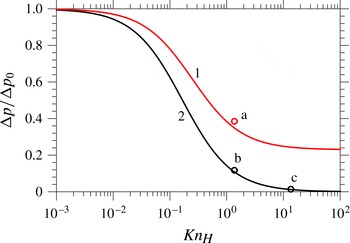
Figure 11. Normalised pressure gradient
 ${\rm\Delta}p/{\rm\Delta}p_{0}$
given as a function of
${\rm\Delta}p/{\rm\Delta}p_{0}$
given as a function of
 $\mathit{Kn}_{H}$
: curve 1,
$\mathit{Kn}_{H}$
: curve 1,
 $A=0$
(in red); curve 2,
$A=0$
(in red); curve 2,
 $A=1$
(in black). The circles labelled a, b and c are the values computed for the pressure gradient at
$A=1$
(in black). The circles labelled a, b and c are the values computed for the pressure gradient at
 ${\tilde{y}}=0.3$
for the cases shown in figure 5(a–c), and these compare well with the predictions of the lubrication analysis.
${\tilde{y}}=0.3$
for the cases shown in figure 5(a–c), and these compare well with the predictions of the lubrication analysis.
These findings help us to understand the results shown in figure 4. For
 $A=1$
, as the ambient pressure is reduced (
$A=1$
, as the ambient pressure is reduced (
 $\bar{P}_{g}\rightarrow 0$
), and hence Maxwell slip is increased (
$\bar{P}_{g}\rightarrow 0$
), and hence Maxwell slip is increased (
 $\mathit{Kn}_{H}\rightarrow \infty$
), the pressure gradient required to pump gas from the contact-line region vanishes, so that the gas offers no resistance to contact-line motion and, consequently, the maximum speed of wetting appears to become unbounded,
$\mathit{Kn}_{H}\rightarrow \infty$
), the pressure gradient required to pump gas from the contact-line region vanishes, so that the gas offers no resistance to contact-line motion and, consequently, the maximum speed of wetting appears to become unbounded,
 $\mathit{Ca}_{c}\rightarrow \infty$
. In contrast, for
$\mathit{Ca}_{c}\rightarrow \infty$
. In contrast, for
 $A=0$
, the lack of slip at the free surface means that gas is always being driven into the contact-line region by the motion of the liquid so that however much
$A=0$
, the lack of slip at the free surface means that gas is always being driven into the contact-line region by the motion of the liquid so that however much
 $\bar{P}_{g}$
is reduced (
$\bar{P}_{g}$
is reduced (
 $\mathit{Kn}_{H}$
increased) a pressure gradient in the gas is always required and
$\mathit{Kn}_{H}$
increased) a pressure gradient in the gas is always required and
 $\mathit{Ca}_{c}$
approaches a finite value based on this.
$\mathit{Ca}_{c}$
approaches a finite value based on this.
4.5. Evaluation of the incompressibility assumption
The analytic expression derived for the pressure gradient in the thin film (4.2) can be used to estimate the validity of the assumptions we have made about the gas flow. In particular, although the flow is clearly low Mach number, compressibility effects in thin films can still be significant, see § 4.5 of Gad-el-Hak (Reference Gad-el-Hak2006). This occurs when the large pressure gradients required to pump gas out of the thin film lead to reductions in pressure that are comparable with the ambient pressure in the gas. As it is the gas flow at the inflection point on the free surface that is most important for air entrainment, we will estimate whether the flow in the gas there is indeed incompressible.
The pressure gradient obtained in (4.2) takes a maximum value of
 ${\rm\Delta}p_{0}=-12\bar{{\it\mu}}/H^{2}$
, as
${\rm\Delta}p_{0}=-12\bar{{\it\mu}}/H^{2}$
, as
 $V\leqslant 1$
, so that the maximum pressure change along a film of length
$V\leqslant 1$
, so that the maximum pressure change along a film of length
 $L_{f}$
is
$L_{f}$
is
 $12\bar{{\it\mu}}L_{f}/H^{2}$
. Simulations show that the film length is never larger than the capillary length, so that
$12\bar{{\it\mu}}L_{f}/H^{2}$
. Simulations show that the film length is never larger than the capillary length, so that
 $L_{f}=1$
is an upper bound. Comparison of the pressure change with the (dimensionless) ambient pressure
$L_{f}=1$
is an upper bound. Comparison of the pressure change with the (dimensionless) ambient pressure
 $P_{g}$
, which is
$P_{g}$
, which is
 $P_{g}=P_{g}^{\star }L^{\star }/({\it\mu}^{\star }U^{\star })$
, gives us that compressibility can be neglected if
$P_{g}=P_{g}^{\star }L^{\star }/({\it\mu}^{\star }U^{\star })$
, gives us that compressibility can be neglected if
 ${\rm\Delta}p_{0}\ll P_{g}$
, which requires
${\rm\Delta}p_{0}\ll P_{g}$
, which requires
 $$\begin{eqnarray}H\gg H_{T}=3.5\sqrt{{\it\mu}_{g}^{\star }U^{\star }/(P_{g}^{\star }L^{\star })},\end{eqnarray}$$
where
 $H_{T}$
is the (dimensionless) transition height below which compressible effects can no longer be neglected. This is consistent with a similar condition derived for drop impact phenomena in Mani et al. (Reference Mani, Mandre and Brenner2010).
$H_{T}$
is the (dimensionless) transition height below which compressible effects can no longer be neglected. This is consistent with a similar condition derived for drop impact phenomena in Mani et al. (Reference Mani, Mandre and Brenner2010).
Taking
 $U^{\star }=1~\text{m}~\text{s}^{-1}$
gives
$U^{\star }=1~\text{m}~\text{s}^{-1}$
gives
 $H_{T}=1.2\times 10^{-3}$
for air at atmospheric pressure, while reducing the pressure by a factor of one hundred gives
$H_{T}=1.2\times 10^{-3}$
for air at atmospheric pressure, while reducing the pressure by a factor of one hundred gives
 $H_{T}=1.2\times 10^{-2}$
. When looking at the values of
$H_{T}=1.2\times 10^{-2}$
. When looking at the values of
 $H$
obtained at various
$H$
obtained at various
 $\mathit{Ca}$
in figure 8 it appears that compressibility may indeed be important. However, the estimate obtained in (4.3) overpredicts
$\mathit{Ca}$
in figure 8 it appears that compressibility may indeed be important. However, the estimate obtained in (4.3) overpredicts
 $H_{T}$
due to (a) neglecting reductions in pressure gradients associated with slip at the interfaces and (b) approximating the film as being a channel of length
$H_{T}$
due to (a) neglecting reductions in pressure gradients associated with slip at the interfaces and (b) approximating the film as being a channel of length
 $L$
and constant height
$L$
and constant height
 $H$
, whereas the film height actually increases by orders of magnitude as one moves away from the contact line, see figure 7. Therefore, before abandoning incompressibility, a more accurate evaluation of this assumption is considered in which the pressure changes along the film obtained from our computations are used instead of
$H$
, whereas the film height actually increases by orders of magnitude as one moves away from the contact line, see figure 7. Therefore, before abandoning incompressibility, a more accurate evaluation of this assumption is considered in which the pressure changes along the film obtained from our computations are used instead of
 ${\rm\Delta}p_{0}$
from (4.2).
${\rm\Delta}p_{0}$
from (4.2).
In figure 12 the variation in
 $p_{g}$
from its far-field value
$p_{g}$
from its far-field value
 $p_{f}$
is plotted as a function of distance from the contact line
$p_{f}$
is plotted as a function of distance from the contact line
 $y-y_{c}$
, along both the gas–solid and gas–liquid interfaces for the cases shown in figure 5(b,c), i.e. for
$y-y_{c}$
, along both the gas–solid and gas–liquid interfaces for the cases shown in figure 5(b,c), i.e. for
 $\bar{P}_{g}=0.14,0.014$
with
$\bar{P}_{g}=0.14,0.014$
with
 $A=1$
. As one would expect in a lubrication flow, the values along the two interfaces are close and are graphically indistinguishable along curve 2. It can be seen that the maximum change in
$A=1$
. As one would expect in a lubrication flow, the values along the two interfaces are close and are graphically indistinguishable along curve 2. It can be seen that the maximum change in
 $p_{g}$
in the thin-film region for the cases considered is 17 and 3 respectively. For the liquid associated with the base state, the substrate speed at
$p_{g}$
in the thin-film region for the cases considered is 17 and 3 respectively. For the liquid associated with the base state, the substrate speed at
 $\mathit{Ca}=0.4$
is
$\mathit{Ca}=0.4$
is
 $U^{\star }=0.16~\text{m}~\text{s}^{-1}$
, so that for
$U^{\star }=0.16~\text{m}~\text{s}^{-1}$
, so that for
 $\bar{P}_{g}=0.014$
, where the gas is most likely to be compressible, we have
$\bar{P}_{g}=0.014$
, where the gas is most likely to be compressible, we have
 $P_{g}=260$
. Therefore, in these cases the pressure change along the film
$P_{g}=260$
. Therefore, in these cases the pressure change along the film
 $p_{g}-p_{f}$
is substantially smaller than the ambient pressure
$p_{g}-p_{f}$
is substantially smaller than the ambient pressure
 $P_{g}$
, with
$P_{g}$
, with
 $(p_{g}-p_{f})/P_{g}<0.012$
.
$(p_{g}-p_{f})/P_{g}<0.012$
.

Figure 12. Deviation of the gas pressure
 $p_{g}$
from its far-field value of
$p_{g}$
from its far-field value of
 $p_{f}$
as a function of distance from the contact line
$p_{f}$
as a function of distance from the contact line
 $y-y_{c}$
, with curves 1 (in black) and 2 (in blue) corresponding to, respectively, the cases considered in figure 5(b,c). The pressure along the gas–solid interface is given by curves 1a, 2a, while 1b, 2b are values from the gas–liquid interface.
$y-y_{c}$
, with curves 1 (in black) and 2 (in blue) corresponding to, respectively, the cases considered in figure 5(b,c). The pressure along the gas–solid interface is given by curves 1a, 2a, while 1b, 2b are values from the gas–liquid interface.
Notably, although the lubrication analysis accurately predicts the pressure gradient in the film, see figure 11, use of the analytic value at the inflection point to estimate the pressure change along the entire length of the thin film is inaccurate. This is due to the widening of the film as one moves away from the contact line. A more accurate estimate could have been achieved by integrating the analytically calculated pressure gradient over the computationally obtained film profile, but a simpler way is to use the computed values of
 $p_{g}$
. Doing this shows that the assumption of incompressibility is an accurate one for the base cases considered. Further simulations confirm that even in the most extreme cases considered here, the incompressibility assumption remains a good one.
$p_{g}$
. Doing this shows that the assumption of incompressibility is an accurate one for the base cases considered. Further simulations confirm that even in the most extreme cases considered here, the incompressibility assumption remains a good one.
5. Parametric study of the system
Having fully analysed the base state, the role of the system parameters is now established by perturbing their values about the base ones. Henceforth, we only consider the most physically relevant case of
 $A=1$
.
$A=1$
.
5.1. Influence of viscosity ratio
The viscosity ratio
 $\bar{{\it\mu}}$
has long been recognised as an important parameter in coating flows as it is a measure of how much resistance the receding gas phase can produce. Working with a dimensionless system allows us to isolate the effect of
$\bar{{\it\mu}}$
has long been recognised as an important parameter in coating flows as it is a measure of how much resistance the receding gas phase can produce. Working with a dimensionless system allows us to isolate the effect of
 $\bar{{\it\mu}}$
on
$\bar{{\it\mu}}$
on
 $\mathit{Ca}_{c}$
, at different ambient pressures, while keeping all other parameters fixed at their base state. The range considered is chosen to cover all values of
$\mathit{Ca}_{c}$
, at different ambient pressures, while keeping all other parameters fixed at their base state. The range considered is chosen to cover all values of
 $\bar{{\it\mu}}$
obtained for the liquids in Benkreira & Khan (Reference Benkreira and Khan2008) used to coat a solid in air, giving
$\bar{{\it\mu}}$
obtained for the liquids in Benkreira & Khan (Reference Benkreira and Khan2008) used to coat a solid in air, giving
 $10^{-4}\leqslant \bar{{\it\mu}}\leqslant 10^{-2}$
.
$10^{-4}\leqslant \bar{{\it\mu}}\leqslant 10^{-2}$
.

Figure 13. Dependence of the critical capillary number
 $\mathit{Ca}_{c}$
on the viscosity ratio
$\mathit{Ca}_{c}$
on the viscosity ratio
 $\bar{{\it\mu}}$
, with all other parameters fixed at their base values: curve 1,
$\bar{{\it\mu}}$
, with all other parameters fixed at their base values: curve 1,
 $\bar{P}_{g}=1$
(black); curve 2,
$\bar{P}_{g}=1$
(black); curve 2,
 $\bar{P}_{g}=0.1$
(red); curve 3,
$\bar{P}_{g}=0.1$
(red); curve 3,
 $\bar{P}_{g}=0.01$
(blue).
$\bar{P}_{g}=0.01$
(blue).
In figure 13 one can see that lower values of the viscosity ratio
 $\bar{{\it\mu}}$
result in higher
$\bar{{\it\mu}}$
result in higher
 $\mathit{Ca}_{c}$
across all values of
$\mathit{Ca}_{c}$
across all values of
 $\bar{P}_{g}$
. What was less expected is that for
$\bar{P}_{g}$
. What was less expected is that for
 $\bar{P}_{g}=0.01$
(curve 3) it appears that there is a value of
$\bar{P}_{g}=0.01$
(curve 3) it appears that there is a value of
 $\bar{{\it\mu}}$
below which
$\bar{{\it\mu}}$
below which
 $\mathit{Ca}_{c}$
increases apparently without bound. This occurs at
$\mathit{Ca}_{c}$
increases apparently without bound. This occurs at
 $\bar{{\it\mu}}=3.3\times 10^{-4}$
, which is slightly less than the base case viscosity ratio (
$\bar{{\it\mu}}=3.3\times 10^{-4}$
, which is slightly less than the base case viscosity ratio (
 $\bar{{\it\mu}}_{0}=3.6\times 10^{-4}$
) where the critical gas pressure
$\bar{{\it\mu}}_{0}=3.6\times 10^{-4}$
) where the critical gas pressure
 $P_{g,c}=9\times 10^{-3}$
. Therefore, at smaller
$P_{g,c}=9\times 10^{-3}$
. Therefore, at smaller
 $\bar{{\it\mu}}$
the critical value
$\bar{{\it\mu}}$
the critical value
 $\bar{P}_{g,c}$
increases, i.e. less pressure reduction is required to reach the critical value.
$\bar{P}_{g,c}$
increases, i.e. less pressure reduction is required to reach the critical value.
The effect of
 $\bar{{\it\mu}}$
on
$\bar{{\it\mu}}$
on
 $\bar{P}_{g,c}$
can be understood by looking back to the lubrication analysis in the previous section and, in particular, the expression for the pressure gradient in the gas (4.2), which is proportional to
$\bar{P}_{g,c}$
can be understood by looking back to the lubrication analysis in the previous section and, in particular, the expression for the pressure gradient in the gas (4.2), which is proportional to
 $\bar{{\it\mu}}$
(in dimensional terms it would be proportional to
$\bar{{\it\mu}}$
(in dimensional terms it would be proportional to
 ${\it\mu}_{g}^{\star }$
). Therefore, while the degree of Maxwell slip controls the boundary conditions to the gas flow, the bulk flow in the gas is characterised by the viscosity ratio
${\it\mu}_{g}^{\star }$
). Therefore, while the degree of Maxwell slip controls the boundary conditions to the gas flow, the bulk flow in the gas is characterised by the viscosity ratio
 $\bar{{\it\mu}}$
, with larger values decreasing
$\bar{{\it\mu}}$
, with larger values decreasing
 $\mathit{Ca}_{c}$
as more effort is required to remove gas from the contact-line region.
$\mathit{Ca}_{c}$
as more effort is required to remove gas from the contact-line region.
5.2. Effect of Ohnesorge number
The effects of inertia are usually assumed to have a negligible influence on the dynamics of air entrainment, with Stokes flow, corresponding to
 $\mathit{Oh}\rightarrow \infty$
, often considered. In full computations of coating flows in Vandre et al. (Reference Vandre, Carvalho and Kumar2013) it was shown that (a) inertial effects in the gas have a negligible influence, reaffirming our assumption that
$\mathit{Oh}\rightarrow \infty$
, often considered. In full computations of coating flows in Vandre et al. (Reference Vandre, Carvalho and Kumar2013) it was shown that (a) inertial effects in the gas have a negligible influence, reaffirming our assumption that
 $\bar{{\it\rho}}=0$
can be taken without loss of generality, and (b) inertial forces in the liquid do not alter
$\bar{{\it\rho}}=0$
can be taken without loss of generality, and (b) inertial forces in the liquid do not alter
 $\mathit{Ca}_{c}$
until they are relatively large. The results in figure 14 at atmospheric pressure agree with these previous conclusions, with a
$\mathit{Ca}_{c}$
until they are relatively large. The results in figure 14 at atmospheric pressure agree with these previous conclusions, with a
 $10^{2}$
reduction in
$10^{2}$
reduction in
 $\mathit{Oh}$
only increasing the value of
$\mathit{Oh}$
only increasing the value of
 $\mathit{Ca}_{c}$
by approximately 10 %. It should be noted that
$\mathit{Ca}_{c}$
by approximately 10 %. It should be noted that
 $\mathit{Ca}_{c}$
at
$\mathit{Ca}_{c}$
at
 $\mathit{Oh}=0.1$
corresponds to
$\mathit{Oh}=0.1$
corresponds to
 $\mathit{Re}=52$
.
$\mathit{Re}=52$
.

Figure 14. The dependence of the critical capillary number
 $\mathit{Ca}_{c}$
on the Ohnesorge number
$\mathit{Ca}_{c}$
on the Ohnesorge number
 $\mathit{Oh}$
with all other parameters fixed at their base values: curve 1,
$\mathit{Oh}$
with all other parameters fixed at their base values: curve 1,
 $\bar{P}_{g}=1$
(black); curve 2,
$\bar{P}_{g}=1$
(black); curve 2,
 $\bar{P}_{g}=0.1$
(red); curve 3,
$\bar{P}_{g}=0.1$
(red); curve 3,
 $\bar{P}_{g}=0.01$
(blue).
$\bar{P}_{g}=0.01$
(blue).
For the lowest ambient pressure
 $\bar{P}_{g}=0.01$
an entirely different behaviour is observed and there is a critical value of
$\bar{P}_{g}=0.01$
an entirely different behaviour is observed and there is a critical value of
 $\mathit{Oh}$
where
$\mathit{Oh}$
where
 $\mathit{Ca}_{c}$
appears to increase without bound. In contrast to the influences of
$\mathit{Ca}_{c}$
appears to increase without bound. In contrast to the influences of
 $\bar{P}_{g}$
and
$\bar{P}_{g}$
and
 $\bar{{\it\mu}}$
which could be rationalised by considering the gas flow, this effect is generated by changes in the liquid dynamics. In particular, in Vandre et al. (Reference Vandre, Carvalho and Kumar2013) it was shown that when inertial effects become more prominent, velocity gradients in the liquid are localised to a thin boundary layer near the moving solid surface and, as a result, the free surface becomes less deformed so that
$\bar{{\it\mu}}$
which could be rationalised by considering the gas flow, this effect is generated by changes in the liquid dynamics. In particular, in Vandre et al. (Reference Vandre, Carvalho and Kumar2013) it was shown that when inertial effects become more prominent, velocity gradients in the liquid are localised to a thin boundary layer near the moving solid surface and, as a result, the free surface becomes less deformed so that
 $\mathit{Ca}_{c}$
increases. Our results show that when combined with small values of
$\mathit{Ca}_{c}$
increases. Our results show that when combined with small values of
 $\bar{P}_{g}$
this mechanism can prevent air entrainment at any
$\bar{P}_{g}$
this mechanism can prevent air entrainment at any
 $\mathit{Ca}$
.
$\mathit{Ca}$
.
5.3. Role of substrate wettability
Experimentally, the wettability of the substrate is known to have an influence on the point of air entrainment both in coating flows and in impact problems, such as the impact of solid spheres on liquid baths (Duez et al.
Reference Duez, Ybert, Clanet and Bocquet2007). In figure 15, our results obtained at constant contact angles
 ${\it\theta}_{d}={\it\theta}_{e}$
, show that the more wettable the substrate, the higher
${\it\theta}_{d}={\it\theta}_{e}$
, show that the more wettable the substrate, the higher
 $\mathit{Ca}_{c}$
is. The curves are from
$\mathit{Ca}_{c}$
is. The curves are from
 $5^{\circ }\leqslant {\it\theta}_{e}\leqslant 175^{\circ }$
to avoid computational difficulties associated with extremely small angles in either phase, but, despite this, the trends are still clear enough. Notably, at reduced pressures variations in
$5^{\circ }\leqslant {\it\theta}_{e}\leqslant 175^{\circ }$
to avoid computational difficulties associated with extremely small angles in either phase, but, despite this, the trends are still clear enough. Notably, at reduced pressures variations in
 $\mathit{Ca}_{c}$
with
$\mathit{Ca}_{c}$
with
 ${\it\theta}_{e}$
are far more dramatic: changing
${\it\theta}_{e}$
are far more dramatic: changing
 ${\it\theta}_{e}$
from
${\it\theta}_{e}$
from
 $30^{\circ }$
to
$30^{\circ }$
to
 $90^{\circ }$
reduces
$90^{\circ }$
reduces
 $\mathit{Ca}_{c}$
by 0.32 at
$\mathit{Ca}_{c}$
by 0.32 at
 $\bar{P}_{g}=0.01$
compared with 0.1 at
$\bar{P}_{g}=0.01$
compared with 0.1 at
 $\bar{P}_{g}=1$
.
$\bar{P}_{g}=1$
.

Figure 15. The dependence of the critical capillary number
 $\mathit{Ca}_{c}$
on the equilibrium contact angle
$\mathit{Ca}_{c}$
on the equilibrium contact angle
 ${\it\theta}_{e}$
with all other parameters fixed at their base values: curve 1,
${\it\theta}_{e}$
with all other parameters fixed at their base values: curve 1,
 $\bar{P}_{g}=1$
(black); curve 2,
$\bar{P}_{g}=1$
(black); curve 2,
 $\bar{P}_{g}=0.1$
(red); curve 3,
$\bar{P}_{g}=0.1$
(red); curve 3,
 $\bar{P}_{g}=0.01$
(blue).
$\bar{P}_{g}=0.01$
(blue).
The model used here predicts that
 $\mathit{Ca}_{c}$
monotonically decreases as
$\mathit{Ca}_{c}$
monotonically decreases as
 ${\it\theta}_{e}$
increases, which is what one may intuitively expect. However, in Blake & De Coninck (Reference Blake and De Coninck2002) the optimal value of
${\it\theta}_{e}$
increases, which is what one may intuitively expect. However, in Blake & De Coninck (Reference Blake and De Coninck2002) the optimal value of
 ${\it\theta}_{e}$
that maximises
${\it\theta}_{e}$
that maximises
 $\mathit{Ca}_{c}$
is not at zero and can even occurs on hydrophobic substrates,
$\mathit{Ca}_{c}$
is not at zero and can even occurs on hydrophobic substrates,
 ${\it\theta}_{e}\geqslant 90^{\circ }$
. It is likely that such effects can only be captured by using a dynamic contact angle model and so this aspect lies beyond the scope of the present paper. However, further experiments at both atmospheric and reduced pressure for solids of different wettabilities would be useful to shed further light on these issues.
${\it\theta}_{e}\geqslant 90^{\circ }$
. It is likely that such effects can only be captured by using a dynamic contact angle model and so this aspect lies beyond the scope of the present paper. However, further experiments at both atmospheric and reduced pressure for solids of different wettabilities would be useful to shed further light on these issues.
5.4. Different gases
Previous studies in both dip coating (Benkreira & Ikin Reference Benkreira and Ikin2010) and drop impact (Xu et al.
Reference Xu, Zhang and Nagel2005) have considered the effect of using different gases on wetting failure. The gases used tend to have a similar viscosity and density at atmospheric pressure to air but possess different molecular weights and hence mean free paths. The fluid flow considered here is incompressible, so that changes in the speed of sound in the gas, and hence the Mach number, do not concern us. However, changes in the mean free path at a given ambient pressure will have an effect on our results. This effect can be accounted for in the results presented, without recomputing everything, by simply rescaling the ambient gas pressure
 $\bar{P}_{g}$
. For example, if a new gas considered has a mean free path
$\bar{P}_{g}$
. For example, if a new gas considered has a mean free path
 $\ell _{atm,n}^{\star }$
that is
$\ell _{atm,n}^{\star }$
that is
 $c$
times larger than that of air at atmospheric pressure, so that
$c$
times larger than that of air at atmospheric pressure, so that
 $\ell _{atm,n}^{\star }=c\ell _{atm}^{\star }$
, then from (1.4) the same
$\ell _{atm,n}^{\star }=c\ell _{atm}^{\star }$
, then from (1.4) the same
 $\mathit{Kn}$
is obtained if we use a rescaled pressure
$\mathit{Kn}$
is obtained if we use a rescaled pressure
 $\bar{P}_{g,n}$
in the new gas that satisfies
$\bar{P}_{g,n}$
in the new gas that satisfies
 $\bar{P}_{g,n}=c\bar{P}_{g}$
.
$\bar{P}_{g,n}=c\bar{P}_{g}$
.
In this way, all the results of the previous section can be used for any gas, rather than just air. For example, if helium is used instead of air, approximately
 $\ell _{atm,\text{He}}^{\star }=3\ell _{atm,air}^{\star }$
, so that
$\ell _{atm,\text{He}}^{\star }=3\ell _{atm,air}^{\star }$
, so that
 $\bar{P}_{g,\text{He}}=3\bar{P}_{g}$
. Then, for the base case considered in § 4.1 the critical pressure was found to be
$\bar{P}_{g,\text{He}}=3\bar{P}_{g}$
. Then, for the base case considered in § 4.1 the critical pressure was found to be
 $\bar{P}_{g}=9\times 10^{-3}$
for air so that for helium this would be increased to
$\bar{P}_{g}=9\times 10^{-3}$
for air so that for helium this would be increased to
 $\bar{P}_{g}=2.7\times 10^{-2}$
. Therefore, as seen experimentally, built into the model is the fact that gases with larger mean free paths require less pressure reduction in order to induce significant non-equilibrium gas effects that increase
$\bar{P}_{g}=2.7\times 10^{-2}$
. Therefore, as seen experimentally, built into the model is the fact that gases with larger mean free paths require less pressure reduction in order to induce significant non-equilibrium gas effects that increase
 $\mathit{Ca}_{c}$
.
$\mathit{Ca}_{c}$
.
5.5. Summary of the parametric study
The effects of non-equilibrium gas dynamics on air entrainment phenomena have been clarified and the role of the various dimensionless parameters on
 $\mathit{Ca}_{c}$
has been characterised by perturbing them about a base case. This has allowed us to isolate the effects of parameters such as
$\mathit{Ca}_{c}$
has been characterised by perturbing them about a base case. This has allowed us to isolate the effects of parameters such as
 $\bar{{\it\mu}}$
which cannot easily be independently varied experimentally. The disadvantage is, of course, that the results cannot easily be used to find, say, the effect of
$\bar{{\it\mu}}$
which cannot easily be independently varied experimentally. The disadvantage is, of course, that the results cannot easily be used to find, say, the effect of
 ${\it\mu}^{\star }$
on coating speeds, as this variable comes into
${\it\mu}^{\star }$
on coating speeds, as this variable comes into
 $\mathit{Ca}$
,
$\mathit{Ca}$
,
 $\mathit{Oh}$
and
$\mathit{Oh}$
and
 $\bar{{\it\mu}}$
, which have thus far been varied independently. Therefore, in the next section we compare our results directly with experiments in Benkreira & Khan (Reference Benkreira and Khan2008) and, in doing so, now step into a dimensional setting.
$\bar{{\it\mu}}$
, which have thus far been varied independently. Therefore, in the next section we compare our results directly with experiments in Benkreira & Khan (Reference Benkreira and Khan2008) and, in doing so, now step into a dimensional setting.
6. Comparison with experimental data: effect of viscosity and gas pressure
We consider now whether the new model is able to account for the influence of the gas pressure
 $P_{g}^{\star }$
on the maximum coating speeds
$P_{g}^{\star }$
on the maximum coating speeds
 $U_{c}^{\star }$
observed in Benkreira & Khan (Reference Benkreira and Khan2008) for different viscosity liquids. All parameters remain unchanged from § 5 except for those that depend on viscosity, namely
$U_{c}^{\star }$
observed in Benkreira & Khan (Reference Benkreira and Khan2008) for different viscosity liquids. All parameters remain unchanged from § 5 except for those that depend on viscosity, namely
 $\mathit{Oh}$
,
$\mathit{Oh}$
,
 $\mathit{Ca}$
and
$\mathit{Ca}$
and
 $\bar{{\it\mu}}$
, which will be based on values used in the experiments of
$\bar{{\it\mu}}$
, which will be based on values used in the experiments of
 ${\it\mu}^{\star }=20$
, 50, 100, 200 mPa s.
${\it\mu}^{\star }=20$
, 50, 100, 200 mPa s.
In figure 16, a direct comparison between the computations and the experimental results in Benkreira & Khan (Reference Benkreira and Khan2008) is shown. Notably, both predict that a significant reduction in
 $P_{g}^{\star }$
from its atmospheric value (
$P_{g}^{\star }$
from its atmospheric value (
 $P_{g,atm}^{\star }=100~\text{kPa}$
) is required to induce increases in
$P_{g,atm}^{\star }=100~\text{kPa}$
) is required to induce increases in
 $U_{c}^{\star }$
, but that once this has been achieved, the subsequent enhancements in
$U_{c}^{\star }$
, but that once this has been achieved, the subsequent enhancements in
 $U_{c}^{\star }$
are substantial. At the lowest viscosity, the agreement is relatively good throughout; however, as is most clear from figure 16(b), one can see that at the higher viscosities, the effect of gas pressure yields enhanced coating speeds earlier in the experiments than in the computations. For example, for the highest viscosity liquid, at
$U_{c}^{\star }$
are substantial. At the lowest viscosity, the agreement is relatively good throughout; however, as is most clear from figure 16(b), one can see that at the higher viscosities, the effect of gas pressure yields enhanced coating speeds earlier in the experiments than in the computations. For example, for the highest viscosity liquid, at
 $P_{g}^{\star }=12~\text{kPa}$
the experimental data (crosses) show that
$P_{g}^{\star }=12~\text{kPa}$
the experimental data (crosses) show that
 $U_{c}^{\star }$
has increased to
$U_{c}^{\star }$
has increased to
 $0.18~\text{m}~\text{s}^{-1}$
from its atmospheric value of
$0.18~\text{m}~\text{s}^{-1}$
from its atmospheric value of
 $0.11~\text{m}~\text{s}^{-1}$
, while the computations, shown by curve 4, only give this degree of enhancement once
$0.11~\text{m}~\text{s}^{-1}$
, while the computations, shown by curve 4, only give this degree of enhancement once
 $P_{g}^{\star }=2~\text{kPa}$
.
$P_{g}^{\star }=2~\text{kPa}$
.

Figure 16. A comparison of our computations for the critical wetting speed
 $U_{c}^{\star }$
as a function of the gas pressure
$U_{c}^{\star }$
as a function of the gas pressure
 $P_{g}^{\star }$
with experimental results obtained in Benkreira & Khan (Reference Benkreira and Khan2008). Curves are computed for liquids of different viscosities
$P_{g}^{\star }$
with experimental results obtained in Benkreira & Khan (Reference Benkreira and Khan2008). Curves are computed for liquids of different viscosities
 ${\it\mu}^{\star }$
: curve 1, 20 mPa s (in red); curve 2, 50 mPa s (in black); curve 3, 100 mPa s (in blue); curve 4, 200 mPa s (in green). The corresponding experimental data are given by, respectively, triangles, diamonds, squares and crosses.
${\it\mu}^{\star }$
: curve 1, 20 mPa s (in red); curve 2, 50 mPa s (in black); curve 3, 100 mPa s (in blue); curve 4, 200 mPa s (in green). The corresponding experimental data are given by, respectively, triangles, diamonds, squares and crosses.
Promisingly, as in the experimental results, curves 1 and 2 cross at low atmospheric pressure, meaning that a higher-viscosity liquid can be coated at faster speeds than a lower one, in contrast to what is observed at atmospheric pressure. Other crossovers may have been observed if higher capillary numbers could have been obtained, as suggested by the path of curve 3. However, the positions of the crossovers do not match the experimental data; while the computed results all appear to cross over around
 $P_{g}^{\star }\sim 1~\text{kPa}$
, the experimental results do so at higher values of
$P_{g}^{\star }\sim 1~\text{kPa}$
, the experimental results do so at higher values of
 $P_{g}^{\star }$
, with the two highest-viscosity solutions crossing over at
$P_{g}^{\star }$
, with the two highest-viscosity solutions crossing over at
 $P_{g}^{\star }\sim 10~\text{kPa}$
.
$P_{g}^{\star }\sim 10~\text{kPa}$
.
In summary, while all of the qualitative features of the experimental results are recovered in our computations, quantitative agreement is not good over the entire range of data. In particular, less pressure reduction is required in the experiments than in the computations for there to be a noticeable effect on the maximum wetting speed. There are a number of possible reasons for this discrepancy, some of which we will now consider.
Roughness of the solid: In Benkreira & Khan (Reference Benkreira and Khan2008) the ‘average peak-to-valley height roughness’ for the experimental results presented is 300 nm. Although this is ‘smooth’ compared with the other solids used in this work, it is still quite rough compared with the solids used in some other coating flow studies. This effect cannot be ignored as experiments in Clarke (Reference Clarke2002) have demonstrated that the roughness of a solid can influence the maximum speed of wetting with, in many cases, faster coating speeds obtained with rougher surfaces.
From a modelling perspective, the level of roughness in the experiments is large when compared with the slip length at the liquid–solid interface
 $l_{s}^{\star }=10~\text{nm}$
. However, simply increasing the value of
$l_{s}^{\star }=10~\text{nm}$
. However, simply increasing the value of
 $l_{s}^{\star }$
in an attempt to mimic the effect of the roughness does not capture the experimental data either. It is likely that the strongest effect of the roughness will be on the actual contact angle, but a theoretical description of this mechanism at high contact-line speeds remains an open problem and is beyond the scope of this work.
$l_{s}^{\star }$
in an attempt to mimic the effect of the roughness does not capture the experimental data either. It is likely that the strongest effect of the roughness will be on the actual contact angle, but a theoretical description of this mechanism at high contact-line speeds remains an open problem and is beyond the scope of this work.
Dynamics of the contact angle: Despite assuming that the contact angle is fixed at its equilibrium value, without fitting the slip length in any way we still obtain reasonable agreement for the values of
 $U_{c}^{\star }$
at atmospheric pressure. This could be a coincidence and dynamic contact angle effects may indeed be important for quantitatively capturing this class of coating flows; however, such effects will not improve the agreement of our present model with experiments. This is because allowing the contact angle to vary will increase the angle from its equilibrium value so that, as shown by the findings of § 5.3,
$U_{c}^{\star }$
at atmospheric pressure. This could be a coincidence and dynamic contact angle effects may indeed be important for quantitatively capturing this class of coating flows; however, such effects will not improve the agreement of our present model with experiments. This is because allowing the contact angle to vary will increase the angle from its equilibrium value so that, as shown by the findings of § 5.3,
 $U_{c}^{\star }$
will decrease for a given pressure. Therefore, although the dynamics of the contact angle will alter our results, it will not explain why
$U_{c}^{\star }$
will decrease for a given pressure. Therefore, although the dynamics of the contact angle will alter our results, it will not explain why
 $\mathit{Ca}_{c}$
increases so quickly with reductions in
$\mathit{Ca}_{c}$
increases so quickly with reductions in
 $\bar{P}_{g}$
and is thus not our main concern here.
$\bar{P}_{g}$
and is thus not our main concern here.
Model for non-equilibrium effects: As shown in § 4.3, the Knudsen number characterising the gas film flow indicated that its dynamics is usually outside the ‘slip regime’ as air entrainment is approached and more complex non-equilibrium gas dynamics should be incorporated. As noted in § 4.3, incorporation of these effects is likely to result in the same qualitative trends but enhanced quantitative ones. In particular, it is likely that less gas will be driven into the contact-line region at a given pressure so that there is an enhancement in
 $\mathit{Ca}_{c}$
at higher ambient pressures, as observed experimentally. Furthermore, this effect will be particularly important at smaller
$\mathit{Ca}_{c}$
at higher ambient pressures, as observed experimentally. Furthermore, this effect will be particularly important at smaller
 $\bar{{\it\mu}}$
, where most of the current discrepancies between theory and experiment appear, as the smaller values of
$\bar{{\it\mu}}$
, where most of the current discrepancies between theory and experiment appear, as the smaller values of
 $H$
obtained there (Vandre et al.
Reference Vandre, Carvalho and Kumar2013) will increase the importance of non-equilibrium effects. Models capable of predicting these effects will be discussed in § 8.
$H$
obtained there (Vandre et al.
Reference Vandre, Carvalho and Kumar2013) will increase the importance of non-equilibrium effects. Models capable of predicting these effects will be discussed in § 8.
The most likely cause of the observed discrepancy seems to be our inadequate description of the gas dynamics, and this aspect will be discussed further in § 8. Before doing so, we consider what consequences our results have for the drop impact phenomenon.
7. Non-equilibrium gas effects in drop impact phenomena
It has previously been suggested (Rein & Delplanque Reference Rein and Delplanque2008), that certain classes of splash observed in drop impact phenomena are triggered by the same mechanisms that cause wetting failure in coating flows. This interpretation is supported by experiments such as those in Driscoll & Nagel (Reference Driscoll and Nagel2011), who find ‘No trapped air beneath the spreading drop outside the small central bubble; there is no significant air film beneath the drop at the time of thin-sheet ejection. This suggests that, rather than an underlying air layer, gas flow at the edge of the spreading drop is responsible for destabilising the liquid.’ This mechanism is shown by figure 1(b). Therefore, we now consider how our results can be related to the more complex unsteady drop impact phenomenon.
The publication that opened up this field of research was Xu et al. (Reference Xu, Zhang and Nagel2005). This work focuses on a threshold ambient pressure
 $P_{T}^{\star }$
that must be achieved in order to suppress splashing for a particular liquid–solid–gas configuration. What is particularly interesting is that for a given impact speed
$P_{T}^{\star }$
that must be achieved in order to suppress splashing for a particular liquid–solid–gas configuration. What is particularly interesting is that for a given impact speed
 $V_{0}^{\star }$
, the threshold pressure strongly depends on the gas, with air, helium, krypton and
$V_{0}^{\star }$
, the threshold pressure strongly depends on the gas, with air, helium, krypton and
 $\text{SF}_{6}$
all used. The data are shown in figure 17, which corresponds in Xu et al. (Reference Xu, Zhang and Nagel2005) to the inset of their figure 2(b). In Xu et al. (Reference Xu, Zhang and Nagel2005), compressibility effects in the gas are assumed to be important when deriving a splash threshold, so that changes in the molecular mass of the gases
$\text{SF}_{6}$
all used. The data are shown in figure 17, which corresponds in Xu et al. (Reference Xu, Zhang and Nagel2005) to the inset of their figure 2(b). In Xu et al. (Reference Xu, Zhang and Nagel2005), compressibility effects in the gas are assumed to be important when deriving a splash threshold, so that changes in the molecular mass of the gases
 $m_{g}^{\star }$
, which alter the speed of sound in the gas, become important and result in a collapse of the data when
$m_{g}^{\star }$
, which alter the speed of sound in the gas, become important and result in a collapse of the data when
 $P_{T}^{\star }$
is scaled by
$P_{T}^{\star }$
is scaled by
 $\sqrt{m_{g}^{\star }/m_{air}^{\star }}$
, where
$\sqrt{m_{g}^{\star }/m_{air}^{\star }}$
, where
 $m_{air}^{\star }$
is the molecular mass of air.
$m_{air}^{\star }$
is the molecular mass of air.

Figure 17. Critical gas pressure
 $P_{T}^{\star }$
required to suppress the splash of a drop with impact speed
$P_{T}^{\star }$
required to suppress the splash of a drop with impact speed
 $V_{0}^{\star }$
with different gases: helium (open circles in green), air (filled circles in blue), krypton (red crosses) and
$V_{0}^{\star }$
with different gases: helium (open circles in green), air (filled circles in blue), krypton (red crosses) and
 $\text{SF}_{6}$
(triangles in black). Obtained from Xu et al. (Reference Xu, Zhang and Nagel2005).
$\text{SF}_{6}$
(triangles in black). Obtained from Xu et al. (Reference Xu, Zhang and Nagel2005).
An alternative explanation is that compressibility effects are negligible and that increased Maxwell slip is responsible for splash suppression at reduced pressure. Given that the mean free path in the gas at the threshold point
 $\ell _{T}^{\star }$
is inversely proportional to both the gas pressure and the square root of the molecular mass
$\ell _{T}^{\star }$
is inversely proportional to both the gas pressure and the square root of the molecular mass
 $\ell _{T}^{\star }\propto (P_{T}^{\star }\sqrt{m_{g}^{\star }})^{-1}$
, to achieve a given
$\ell _{T}^{\star }\propto (P_{T}^{\star }\sqrt{m_{g}^{\star }})^{-1}$
, to achieve a given
 $\ell _{T}^{\star }$
, increases in
$\ell _{T}^{\star }$
, increases in
 $m_{g}^{\star }$
require decreases in
$m_{g}^{\star }$
require decreases in
 $P_{T}^{\star }$
. In other words, gases with higher molecular mass will need lower pressures to suppress splashing, as seen in Xu et al. (Reference Xu, Zhang and Nagel2005).
$P_{T}^{\star }$
. In other words, gases with higher molecular mass will need lower pressures to suppress splashing, as seen in Xu et al. (Reference Xu, Zhang and Nagel2005).
The dimensionless number characterising the level of Maxwell slip at a given threshold pressure in the gas is the Knudsen number
 $\mathit{Kn}_{T}=\ell _{T}^{\star }/R^{\star }$
, where
$\mathit{Kn}_{T}=\ell _{T}^{\star }/R^{\star }$
, where
 $R^{\star }=1.7~\text{mm}$
is the drop radius. Using the properties of air, the expression for
$R^{\star }=1.7~\text{mm}$
is the drop radius. Using the properties of air, the expression for
 $\mathit{Kn}_{T}$
required is
$\mathit{Kn}_{T}$
required is
 $$\begin{eqnarray}\mathit{Kn}_{T}=\frac{\mathit{Kn}_{air,atm}}{\sqrt{\tilde{m}_{g}}\bar{P}_{T}},\quad \text{where }\bar{P}_{T}=\frac{P_{T}^{\star }}{P_{atm}^{\star }}\text{ and }\tilde{m}_{g}=\frac{m_{g}^{\star }}{m_{air}^{\star }},\end{eqnarray}$$
where the coefficient of proportionality
 $\mathit{Kn}_{air,atm}=4.1\times 10^{-5}$
is the Knudsen number of air at atmospheric pressure and the molecular weights in daltons of
$\mathit{Kn}_{air,atm}=4.1\times 10^{-5}$
is the Knudsen number of air at atmospheric pressure and the molecular weights in daltons of
 $m_{He}^{\star }=4$
,
$m_{He}^{\star }=4$
,
 $m_{air}^{\star }=29$
,
$m_{air}^{\star }=29$
,
 $m_{\text{Kr}}^{\star }=83.8$
and
$m_{\text{Kr}}^{\star }=83.8$
and
 $m_{\text{SF}_{6}}^{\star }=146$
can be taken from Xu et al. (Reference Xu, Zhang and Nagel2005). As for the coating flow analysis, the value of the Knudsen number has to be based on the global characteristics of the flow and would be larger if it could have been derived from the appropriate length scales near the moving contact line.
$m_{\text{SF}_{6}}^{\star }=146$
can be taken from Xu et al. (Reference Xu, Zhang and Nagel2005). As for the coating flow analysis, the value of the Knudsen number has to be based on the global characteristics of the flow and would be larger if it could have been derived from the appropriate length scales near the moving contact line.
Ideally, the collapse of data would use
 $\mathit{Kn}_{T}$
and a capillary number based on the contact-line speed
$\mathit{Kn}_{T}$
and a capillary number based on the contact-line speed
 $U^{\star }$
at the point of air entrainment, as considered for the coating flow analysis. However, such measurements were not made in the experimental work so we shall instead base the capillary number
$U^{\star }$
at the point of air entrainment, as considered for the coating flow analysis. However, such measurements were not made in the experimental work so we shall instead base the capillary number
 $\mathit{Ca}_{V_{0}^{\star }}$
on the impact speed
$\mathit{Ca}_{V_{0}^{\star }}$
on the impact speed
 $V_{0}^{\star }$
, an assumption that will be discussed in § 8.
$V_{0}^{\star }$
, an assumption that will be discussed in § 8.
In figure 18, the raw data from figure 17 are shown to collapse well onto axes of
 $\mathit{Ca}_{V_{0}^{\star }}$
versus
$\mathit{Ca}_{V_{0}^{\star }}$
versus
 $\mathit{Kn}_{T}$
. This is encouraging, and suggests that non-equilibrium effects in the gas may be important for drop impact phenomena. It is particularly reassuring to see that the capillary numbers obtained are within the range one may expect for air entrainment phenomena to be occurring, although the capillary number based on the contact-line speed at the entrainment point may be much larger. Ideally, changes in the viscosity of the liquid would also be included into the data collapse, as achieved in Xu et al. (Reference Xu, Zhang and Nagel2005), but this is not possible here as such variations cannot simply be absorbed into the capillary number, but will also alter many other dominant parameters such as the viscosity ratio.
$\mathit{Kn}_{T}$
. This is encouraging, and suggests that non-equilibrium effects in the gas may be important for drop impact phenomena. It is particularly reassuring to see that the capillary numbers obtained are within the range one may expect for air entrainment phenomena to be occurring, although the capillary number based on the contact-line speed at the entrainment point may be much larger. Ideally, changes in the viscosity of the liquid would also be included into the data collapse, as achieved in Xu et al. (Reference Xu, Zhang and Nagel2005), but this is not possible here as such variations cannot simply be absorbed into the capillary number, but will also alter many other dominant parameters such as the viscosity ratio.

Figure 18. Critical Knudsen number
 $\mathit{Kn}_{T}$
, scaled by its value in air at atmospheric pressure, required to suppress the splash of a drop whose capillary-number-based impact speed is
$\mathit{Kn}_{T}$
, scaled by its value in air at atmospheric pressure, required to suppress the splash of a drop whose capillary-number-based impact speed is
 $\mathit{Ca}_{V_{0}^{\star }}$
. The collapse of data from figure 17 onto a single curve is apparent.
$\mathit{Ca}_{V_{0}^{\star }}$
. The collapse of data from figure 17 onto a single curve is apparent.
Although the data collapse looks impressive, a number of outstanding questions remain. First, as also seen in § 6, experimentally only relatively small changes in atmospheric pressure are required to suppress splashing, with a factor of 10 decrease sufficient to prevent it in all cases considered here (figure 17), and it remains to be seen whether the Maxwell-slip model is able to predict such a large effect at these reduced pressures. Second, in this framework it is not obvious why the drop spreads for some distance before splashing, when the largest contact-line speeds are obtained earliest in the impact process. These two issues will be addressed in § 8 and will require further experimental and theoretical work before they can be fully resolved.
8. Discussion
It has been shown that non-equilibrium effects in a gas, influencing the flow through Maxwell slip at boundaries, can substantially increase the critical speed at which air entrainment occurs. Notably, neglecting to use slip at the gas–liquid boundary produces qualitatively different results from those obtained when slip is allowed, predicting a finite, rather than unbounded, maximum speed of wetting as the pressure is reduced. Importantly, the problem has been formulated locally, so that the model is valid for any shape of the gas domain and remains accurate both far away from the gas film, where non-equilibrium gas effects will have a negligible influence on the overall flow, as well as very close to the contact line, where regions of high curvature invalidate the lubrication approximation.
The model proposed was shown to reproduce many of the features of the experimental results in Benkreira & Khan (Reference Benkreira and Khan2008) but failed to accurately predict the ambient pressures at which coating speeds begin to rise for the higher-viscosity liquids. These observations open up a number of potential areas for experimental and theoretical research which will now be considered.
8.1. Extension of the non-equilibrium gas model
General research into non-equilibrium gas dynamics has identified different ‘regimes’ of flow which indicate the modelling approach that should be used. Application of these to the flow in the gas film, characterised by
 $\mathit{Kn}_{H}$
, gives the following.
$\mathit{Kn}_{H}$
, gives the following.
Conventional regime (
 $\mathit{Kn}_{H}<10^{-3}$
): The Navier–Stokes equations with no-slip at solid surfaces provide an accurate representation of the gas flow.
$\mathit{Kn}_{H}<10^{-3}$
): The Navier–Stokes equations with no-slip at solid surfaces provide an accurate representation of the gas flow.
Slip regime (
 $10^{-3}<Kn_{H}<10^{-1}$
): Non-equilibrium effects become significant close to the boundary so that the no-slip condition must be relaxed to allow for Maxwell slip.
$10^{-3}<Kn_{H}<10^{-1}$
): Non-equilibrium effects become significant close to the boundary so that the no-slip condition must be relaxed to allow for Maxwell slip.
Transition regime (
 $10^{-1}<Kn_{H}<10$
): Knudsen layers occupy significant proportions of the domain and kinetic theory is required to provide reliable predictions.
$10^{-1}<Kn_{H}<10$
): Knudsen layers occupy significant proportions of the domain and kinetic theory is required to provide reliable predictions.
Free molecular flow regime (
 $\mathit{Kn}_{H}>10$
): Molecular collisions become rare so that the collision operator in the Boltzmann equation can be neglected.
$\mathit{Kn}_{H}>10$
): Molecular collisions become rare so that the collision operator in the Boltzmann equation can be neglected.
Clearly, identification of which regime is important for the dynamic wetting problems of interest will be key to deciding which methods should be implemented.
The Knudsen numbers recovered for the gas film flow show that in many cases the model proposed in § 2 has been used outside its limits of applicability. In particular, once in the transition regime the effect of Knudsen layers can no longer be accurately captured by a first-order slip condition, as assumed here. An entire hierarchy of approaches of varying complexity have been proposed in the published literature to overcome this inadequacy, and which of these is optimum for the class of problem considered here is, at present, unclear. A sensible first step would be to remain within a continuum framework and to incorporate more advanced non-equilibrium gas effects either, in the simplest case, by using a second-order slip condition, such as that proposed in Hadjiconstantinou (Reference Hadjiconstantinou2003), or, at the next level of difficulty, by modifying the bulk constitutive relations also (Lockerby, Reese & Gallis Reference Lockerby, Reese and Gallis2005a ). Research in this direction is currently underway.
The regions of applicability of the aforementioned approaches are often unclear, and the only way to test these is to compare with solutions obtained from the Boltzmann equation. This can now be routinely achieved using a variety of methods, with the direct simulation Monte Carlo (DSMC) approach being popular (Bird Reference Bird1994). However, in this setting it is not clear how the liquid–gas free surface should be treated as the Boltzmann equation cannot be applied across the boundary and into the liquid phase. Whether some plausible assumptions about the liquid free-surface properties could be made or whether DSMC in the gas could somehow be coupled to molecular dynamics simulations (Koplik & Banavar Reference Koplik and Banavar1995) in the bulk of the liquid remains to be seen. Progress in the latter area would shed light on not only the bulk flow of the gas, but also its interaction with boundaries formed by liquids.
8.2. Alternative flow configurations
It is of interest to look at the effects of gas pressure on coating speeds in a range of different set-ups, both experimentally and theoretically. In particular, the effects of confinement, where the contact line is isolated by a nearby boundary, have not been considered, and neither have axisymmetric geometries such as those used in fibre coating.
The fibre coating configuration is particularly interesting as experiments in Simpkins & Kuck (Reference Simpkins and Kuck2003) show that extremely high capillary numbers can be achieved before air entrainment occurs and, at present, the precise cause for this remains to be seen. Some works claim that the same mechanism has been observed in hydrodynamic assist (Blake, Dobson & Ruschak Reference Blake, Dobson and Ruschak2004), while others have proposed that air is actually entrained into the liquid but then dissolved due to the high pressures there (Jacqmin Reference Jacqmin2002). Incorporation of the models proposed into the computational framework developed here should allow one to distinguish between these rival interpretations.
8.3. Development of analytic theory
The theory of Cox (Reference Cox1986) has been used widely to calculate an apparent contact angle from its actual value in both single- and two-phase dynamic wetting phenomena. Although this theory is based on a small-capillary-number asymptotics, so that it lacks accuracy for many coating flows (Vandre et al.
Reference Vandre, Carvalho and Kumar2013), it nevertheless has been a useful tool for interpreting experiments and predicts a possible mechanism by which air entrainment can occur; namely, that once the apparent angle reaches
 $180^{\circ }$
, no more solutions can be obtained. However, in its present state this theory cannot capture the phenomena investigated in this paper.
$180^{\circ }$
, no more solutions can be obtained. However, in its present state this theory cannot capture the phenomena investigated in this paper.
Cox’s theory contains an ‘inner region’ where additional effects come into play, such as slip, which allow the moving contact-line problem to be circumvented. When one has the same slip length in each phase, then the theory is valid, but for the problems we have considered the slip in the gas phase is many times larger than that in the liquid. In particular, the slip length in the gas phase is likely to become comparable with the scale of the ‘intermediate region’, where the bending of the free surface occurs, so that the entire asymptotic structure of the problem becomes unclear. It would be of interest to see whether Cox’s approach can be generalised for this more complex class of flows.
8.4. Parametric experimental study of dip coating at reduced pressures
The results of Benkreira & Khan (Reference Benkreira and Khan2008) have allowed us to compare our computational results with experimental data. However, these are, at present, the only results in the published literature considering the effect of gas pressure on coating processes. Therefore, additional experimental studies would be useful in order to develop the theory of this class of problems. Such an investigation could, for example, use a wider variety of liquids and consider solids with a range of different wettabilities and/or roughnesses. Furthermore, consideration of how accelerating or decelerating the plate alters the flow may give some initial insight into more complex unsteady flows such as drop impact.
If the aforementioned analyses could be combined with modern experimental techniques, such as interferometry measurements, then some details of the gas film profile could potentially be recovered, as has been achieved in drop impact phenomena. These results would provide an excellent benchmark for any potential theories to be compared with.
8.5. Drop impact and spreading
Drop impact phenomena are notoriously difficult to capture computationally due to the inherently multiscale nature of a problem that involves unsteady large deformation of the flow domain. Although this has been achieved in the case of a single-phase flow, e.g. in Sprittles & Shikhmurzaev (Reference Sprittles and Shikhmurzaev2012b ), at present there are no codes that have captured all physical scales in (a) the dynamics of impact, where a thin gas film cushions the falling drop, (b) the topological change, when the drop first touches the solid, and (c) the spreading process, where the slip length needs to be resolved. The construction of a code capable of achieving this goal is highly sought after.
A question arising from our analysis in § 7 is why the drop spreads for some distance before splashing, when its highest speeds are obtained early on in the impact process. The answer to this question is likely to involve the shape of the drop and its flow field, so that one cannot simply consider an isolated moving contact line, as we have done, but must also consider the outer influence of the flow field on the point at which air entrainment occurs.
The situation with drop impact could be similar to that of curtain coating, where the point at which air entrainment occurs is dependent not only on the contact-line speed, but also on the flow geometry (Blake, Clarke & Ruschak Reference Blake, Clarke and Ruschak1994; Clarke & Stattersfield Reference Clarke and Stattersfield2006). In particular, when the contact line is below the falling liquid curtain it appears to be ‘assisted’ by the downward pressure of the curtain (Blake et al. Reference Blake, Dobson and Ruschak2004), which prevents air entrainment, while if a heel forms in the free surface the contact line becomes isolated from the bulk flow and there is no assist. Similarly, in drop impact, during the initial stages of spreading the contact line is located below the drop, and thus wetting is assisted by the downward pressure of the bulk flow, until a lamella is ejected, analogous to a heel in curtain coating. At this point, the contact line is isolated and air entrainment between the lamella and the substrate is able to lift off a sheet of liquid which creates a splash.
In order to determine whether the aforementioned mechanism is the correct one for drop impact phenomena, it may still be useful to use the simpler coating flow set-ups. One possibility is that the influence of an impulsively started or accelerating plate could be considered in such a manner as to mimic the impact process. Another avenue of enquiry would be to alter the flow domain to mimic the flux of mass arriving at the contact line in drop impact phenomena.
From an experimental perspective, it would be extremely useful to know the contact-line speed at the point of air entrainment, so that the capillary numbers used in § 7 could be based on this, rather than the impact speed. In particular, if air entrainment occurs after the drop contact line has moved a radius
 $r_{s}^{\star }$
, and the contact line moves with a square root in time dependence, as shown experimentally (Riboux & Gordillo Reference Riboux and Gordillo2014) for the initial stages of motion, so that
$r_{s}^{\star }$
, and the contact line moves with a square root in time dependence, as shown experimentally (Riboux & Gordillo Reference Riboux and Gordillo2014) for the initial stages of motion, so that
 $r_{s}^{\star }/R^{\star }=A\sqrt{V_{0}^{\star }t^{\star }/R^{\star }}$
and
$r_{s}^{\star }/R^{\star }=A\sqrt{V_{0}^{\star }t^{\star }/R^{\star }}$
and
 $U^{\star }/V_{0}^{\star }=A/2\sqrt{R^{\star }/(V_{0}^{\star }t^{\star })}$
, where
$U^{\star }/V_{0}^{\star }=A/2\sqrt{R^{\star }/(V_{0}^{\star }t^{\star })}$
, where
 $A$
is a constant, we find that
$A$
is a constant, we find that
 $U^{\star }/V_{0}^{\star }=(A^{2}/2)R^{\star }/r_{s}^{\star }$
. Therefore,
$U^{\star }/V_{0}^{\star }=(A^{2}/2)R^{\star }/r_{s}^{\star }$
. Therefore,
 $\mathit{Ca}_{V_{0}^{\star }}$
is only a fixed multiple of
$\mathit{Ca}_{V_{0}^{\star }}$
is only a fixed multiple of
 $\mathit{Ca}$
if air entrainment always occurs at the same radius
$\mathit{Ca}$
if air entrainment always occurs at the same radius
 $r_{s}^{\star }$
, which seems unlikely to be the case across all parameter space. Therefore, we cannot be sure that
$r_{s}^{\star }$
, which seems unlikely to be the case across all parameter space. Therefore, we cannot be sure that
 $\mathit{Ca}_{c}\propto \mathit{Ca}_{V_{0}^{\star }}$
and more experimental data are indeed required.
$\mathit{Ca}_{c}\propto \mathit{Ca}_{V_{0}^{\star }}$
and more experimental data are indeed required.

Figure 19. Dependence of the elevation
 ${\rm\Delta}y$
and maximum apparent contact angle
${\rm\Delta}y$
and maximum apparent contact angle
 ${\it\theta}_{M}$
on the capillary number
${\it\theta}_{M}$
on the capillary number
 $\mathit{Ca}$
for
$\mathit{Ca}$
for
 $\bar{{\it\mu}}=1,10^{-1};2,10^{-2};3,10^{-3};4,10^{-4}$
and other parameters listed in the text. The dashed lines indicate the critical capillary number
$\bar{{\it\mu}}=1,10^{-1};2,10^{-2};3,10^{-3};4,10^{-4}$
and other parameters listed in the text. The dashed lines indicate the critical capillary number
 $\mathit{Ca}=\mathit{Ca}_{c}$
past which no steady-state solutions exist.
$\mathit{Ca}=\mathit{Ca}_{c}$
past which no steady-state solutions exist.
Acknowledgements
The author would like to thank T. Blake and Y. Shikhmurzaev for numerous insightful discussions and continual encouragement over the years, D. Lockerby for lending his expertise with aspects of the gas dynamics, E. Vandre for stimulating conversations about coating flows, and the referees of the paper whose valuable comments helped to improve the manuscript.
Appendix A. Benchmark calculations
From a theoretical perspective, both extended lubrication theory (Chan et al.
Reference Chan, Srivastava, Marchand, Andreotti, Biferale, Toschi and Snoeijer2013) and full computations (Vandre et al.
Reference Vandre, Carvalho and Kumar2012, Reference Vandre, Carvalho and Kumar2013) have identified a critical capillary number past which no steady two-dimensional solutions exist, and it has been assumed that this corresponds to the
 $\mathit{Ca}_{c}$
observed in experiments. As initially observed for the plate withdrawal problem, i.e. the dewetting scenario (Snoeijer et al.
Reference Snoeijer, Andreotti, Delon and Fermigier2007), the turning point at
$\mathit{Ca}_{c}$
observed in experiments. As initially observed for the plate withdrawal problem, i.e. the dewetting scenario (Snoeijer et al.
Reference Snoeijer, Andreotti, Delon and Fermigier2007), the turning point at
 $\mathit{Ca}_{c}$
in the map of elevation
$\mathit{Ca}_{c}$
in the map of elevation
 ${\rm\Delta}y$
(or maximum apparent contact angle
${\rm\Delta}y$
(or maximum apparent contact angle
 ${\it\theta}_{M}$
) versus
${\it\theta}_{M}$
) versus
 $\mathit{Ca}$
separates stable and unstable branches of steady-state solutions (figure 19). Consequently, when considering the entire solution space, for certain
$\mathit{Ca}$
separates stable and unstable branches of steady-state solutions (figure 19). Consequently, when considering the entire solution space, for certain
 $\mathit{Ca}$
multiple values of elevation
$\mathit{Ca}$
multiple values of elevation
 ${\rm\Delta}y$
exist, and no function
${\rm\Delta}y$
exist, and no function
 ${\rm\Delta}y={\rm\Delta}y(\mathit{Ca})$
exists. Notably though, along all sections of the solution path we have
${\rm\Delta}y={\rm\Delta}y(\mathit{Ca})$
exists. Notably though, along all sections of the solution path we have
 $\mathit{Ca}<\mathit{Ca}_{c}$
, so that
$\mathit{Ca}<\mathit{Ca}_{c}$
, so that
 $\mathit{Ca}_{c}$
is indeed the maximum speed of wetting.
$\mathit{Ca}_{c}$
is indeed the maximum speed of wetting.
In order to determine
 $\mathit{Ca}_{c}$
for a given system, a number of possible solution techniques exist. The most obvious approach is to find a solution at a relatively small
$\mathit{Ca}_{c}$
for a given system, a number of possible solution techniques exist. The most obvious approach is to find a solution at a relatively small
 $\mathit{Ca}$
, then increase its value, using the previous computed solution as an initial guess for the next
$\mathit{Ca}$
, then increase its value, using the previous computed solution as an initial guess for the next
 $\mathit{Ca}$
, and repeat until no more steady-state solutions exist. This is the simplest method and reliably finds
$\mathit{Ca}$
, and repeat until no more steady-state solutions exist. This is the simplest method and reliably finds
 $\mathit{Ca}_{c}$
, but it does not allow us to extract the solution path past the critical point where
$\mathit{Ca}_{c}$
, but it does not allow us to extract the solution path past the critical point where
 $\mathit{Ca}<\mathit{Ca}_{c}$
, as noted in Vandre et al. (Reference Vandre, Carvalho and Kumar2012). A different approach, which allows the entire solution path to be captured, is to determine
$\mathit{Ca}<\mathit{Ca}_{c}$
, as noted in Vandre et al. (Reference Vandre, Carvalho and Kumar2012). A different approach, which allows the entire solution path to be captured, is to determine
 $\mathit{Ca}$
, i.e. treat it as an unknown in the problem, for a fixed elevation of the contact line
$\mathit{Ca}$
, i.e. treat it as an unknown in the problem, for a fixed elevation of the contact line
 ${\rm\Delta}y$
. This approach works better in practice, as for every
${\rm\Delta}y$
. This approach works better in practice, as for every
 ${\rm\Delta}y$
, there is a unique
${\rm\Delta}y$
, there is a unique
 $\mathit{Ca}$
, i.e. there is a function
$\mathit{Ca}$
, i.e. there is a function
 $\mathit{Ca}=\mathit{Ca}({\rm\Delta}y)$
. Consequently, curves like those in figure 19 can be generated.
$\mathit{Ca}=\mathit{Ca}({\rm\Delta}y)$
. Consequently, curves like those in figure 19 can be generated.

Figure 20. Free-surface profiles for the case of
 $\bar{{\it\mu}}=10^{-3}$
at different elevations: 1,
$\bar{{\it\mu}}=10^{-3}$
at different elevations: 1,
 ${\rm\Delta}y=-0.5$
; 2,
${\rm\Delta}y=-0.5$
; 2,
 ${\rm\Delta}y=-1$
; 3,
${\rm\Delta}y=-1$
; 3,
 ${\rm\Delta}y=-1.5$
; 4,
${\rm\Delta}y=-1.5$
; 4,
 ${\rm\Delta}y=-2$
; 5,
${\rm\Delta}y=-2$
; 5,
 ${\rm\Delta}y=-2.5$
; 6,
${\rm\Delta}y=-2.5$
; 6,
 ${\rm\Delta}y=-3$
.
${\rm\Delta}y=-3$
.
In principle, as much of the unstable branch as required can be captured, but for
 ${\rm\Delta}y\ll {\rm\Delta}y_{crit}$
, where
${\rm\Delta}y\ll {\rm\Delta}y_{crit}$
, where
 ${\rm\Delta}y_{crit}$
is the elevation when
${\rm\Delta}y_{crit}$
is the elevation when
 $\mathit{Ca}=\mathit{Ca}_{c}$
, the deformation of the free surface becomes large and this process becomes computationally intensive, particularly at small
$\mathit{Ca}=\mathit{Ca}_{c}$
, the deformation of the free surface becomes large and this process becomes computationally intensive, particularly at small
 $\bar{{\it\mu}}$
. Consequently, simulations were run up to the point in the solution path where the mesh failed, usually due to the finite elements becoming too distorted, and stopped there. As one can see from figure 19, all simulations were extended well past
$\bar{{\it\mu}}$
. Consequently, simulations were run up to the point in the solution path where the mesh failed, usually due to the finite elements becoming too distorted, and stopped there. As one can see from figure 19, all simulations were extended well past
 ${\rm\Delta}y={\rm\Delta}y_{crit}$
, and it was only the smallest viscosity ratio (curve 4) where the code finished prematurely, i.e. before
${\rm\Delta}y={\rm\Delta}y_{crit}$
, and it was only the smallest viscosity ratio (curve 4) where the code finished prematurely, i.e. before
 ${\rm\Delta}y=-3$
.
${\rm\Delta}y=-3$
.
A.1. Calculations and comparison with Vandre et al. (Reference Vandre, Carvalho and Kumar2013)
In order to compare our computations with previous work in Vandre et al. (Reference Vandre, Carvalho and Kumar2013), consider Stokes flow
 $\mathit{Oh}^{-1}=0$
, with the slip lengths of the liquid–solid and gas–solid interfaces equal at
$\mathit{Oh}^{-1}=0$
, with the slip lengths of the liquid–solid and gas–solid interfaces equal at
 $l_{s}=\mathit{Kn}=10^{-4}$
, no-slip across the liquid–gas interface, so that
$l_{s}=\mathit{Kn}=10^{-4}$
, no-slip across the liquid–gas interface, so that
 $A=0$
, and a constant contact angle of
$A=0$
, and a constant contact angle of
 ${\it\theta}_{d}=90^{\circ }$
. Using these parameters, the critical capillary number
${\it\theta}_{d}=90^{\circ }$
. Using these parameters, the critical capillary number
 $\mathit{Ca}_{c}$
and maximum apparent contact angle at this point
$\mathit{Ca}_{c}$
and maximum apparent contact angle at this point
 ${\it\theta}_{M}$
, which occurs at the inflection point on the free surface (see figure 2), are computed for different viscosity ratios
${\it\theta}_{M}$
, which occurs at the inflection point on the free surface (see figure 2), are computed for different viscosity ratios
 $\bar{{\it\mu}}=10^{-1},10^{-2},10^{-3},10^{-4}$
and compared with the results in Vandre et al. (Reference Vandre, Carvalho and Kumar2013).
$\bar{{\it\mu}}=10^{-1},10^{-2},10^{-3},10^{-4}$
and compared with the results in Vandre et al. (Reference Vandre, Carvalho and Kumar2013).
In figure 19, the dependences of
 ${\rm\Delta}y$
and
${\rm\Delta}y$
and
 ${\it\theta}_{M}$
on
${\it\theta}_{M}$
on
 $\mathit{Ca}$
are computed. From the curves one can clearly see the existence of a critical capillary number
$\mathit{Ca}$
are computed. From the curves one can clearly see the existence of a critical capillary number
 $\mathit{Ca}_{c}$
past which (
$\mathit{Ca}_{c}$
past which (
 $\mathit{Ca}>\mathit{Ca}_{c}$
) no solutions exist. On further decreasing
$\mathit{Ca}>\mathit{Ca}_{c}$
) no solutions exist. On further decreasing
 ${\rm\Delta}y$
, so that the contact line moves further down the plate, solutions are recovered for which
${\rm\Delta}y$
, so that the contact line moves further down the plate, solutions are recovered for which
 $\mathit{Ca}<\mathit{Ca}_{c}$
, and the capillary number begins to oscillate around a capillary number
$\mathit{Ca}<\mathit{Ca}_{c}$
, and the capillary number begins to oscillate around a capillary number
 $\mathit{Ca}^{\ast }<\mathit{Ca}_{c}$
as also observed in theoretical works on dewetting phenomena, where these solutions have been shown to correspond to a series of saddle–node bifurcations, see figures 4 and 5 of Snoeijer et al. (Reference Snoeijer, Andreotti, Delon and Fermigier2007), which are related to transient states (Snoeijer et al.
Reference Snoeijer, Delon, Fermigier and Andreotti2006).
$\mathit{Ca}^{\ast }<\mathit{Ca}_{c}$
as also observed in theoretical works on dewetting phenomena, where these solutions have been shown to correspond to a series of saddle–node bifurcations, see figures 4 and 5 of Snoeijer et al. (Reference Snoeijer, Andreotti, Delon and Fermigier2007), which are related to transient states (Snoeijer et al.
Reference Snoeijer, Delon, Fermigier and Andreotti2006).
Similar oscillations are observed for
 ${\it\theta}_{M}$
, where, notably, along the unstable branch the maximum apparent angle can increase beyond
${\it\theta}_{M}$
, where, notably, along the unstable branch the maximum apparent angle can increase beyond
 $180^{\circ }$
. This can be seen in figure 20, where between curves 3 and 4 a hump develops in the free-surface profile. In this region, the gradient of the free surface is negative so that the angle that this portion makes with the solid, i.e. the apparent angle, gives a maximum of
$180^{\circ }$
. This can be seen in figure 20, where between curves 3 and 4 a hump develops in the free-surface profile. In this region, the gradient of the free surface is negative so that the angle that this portion makes with the solid, i.e. the apparent angle, gives a maximum of
 ${\it\theta}_{M}>180^{\circ }$
.
${\it\theta}_{M}>180^{\circ }$
.
A comparison between the critical capillary numbers computed in Vandre et al. (Reference Vandre, Carvalho and Kumar2013) and those observed here is not likely to be exact, as different flow geometries have been used. However, in cases where
 $\mathit{Ca}_{c}$
is not too large and the effect of the flow geometry is relatively weak we may expect our values to be comparable with theirs. In table 2 this is shown to be the case. The computed values of both
$\mathit{Ca}_{c}$
is not too large and the effect of the flow geometry is relatively weak we may expect our values to be comparable with theirs. In table 2 this is shown to be the case. The computed values of both
 $\mathit{Ca}_{c}$
and
$\mathit{Ca}_{c}$
and
 ${\it\theta}_{M}$
at this capillary number, which is a very sensitive measure, agree well across a large range of viscosity ratios. It is not our intention to analyse these data in detail, as this has already been achieved in Vandre et al. (Reference Vandre, Carvalho and Kumar2013), but this table will be useful as a benchmark for future computational work in this area.
${\it\theta}_{M}$
at this capillary number, which is a very sensitive measure, agree well across a large range of viscosity ratios. It is not our intention to analyse these data in detail, as this has already been achieved in Vandre et al. (Reference Vandre, Carvalho and Kumar2013), but this table will be useful as a benchmark for future computational work in this area.
Table 2. Comparison of the critical capillary number
 $\mathit{Ca}_{c}$
and free-surface angle at the inflection point
$\mathit{Ca}_{c}$
and free-surface angle at the inflection point
 ${\it\theta}_{M}$
obtained from our code with those obtained in Vandre et al. (Reference Vandre, Carvalho and Kumar2013) across a range of viscosity ratios
${\it\theta}_{M}$
obtained from our code with those obtained in Vandre et al. (Reference Vandre, Carvalho and Kumar2013) across a range of viscosity ratios
 $\bar{{\it\mu}}$
.
$\bar{{\it\mu}}$
.


