


1. Introduction
Wings in the wakes of upstream bodies are of great interest in aerodynamics, biologically inspired flows and energy harvesting. Fixed tandem wings found on aircraft canard-wing configurations (Scharpf & Mueller Reference Scharpf and Mueller1992), some formation flight configurations (Bangash, Sanchez & Ahmed Reference Bangash, Sanchez and Ahmed2006), aircraft wings during flight refuelling from another aircraft and aircraft wings in ship airwakes are typical examples of fixed wings in wakes. Rotor blades passing through the wakes of stator blades in turbomachinery (Hodson & Howell Reference Hodson and Howell2005), wind turbines and airfoil sections downstream of a propeller have similarities to the fixed-wing cases. Wakes are generally turbulent in all these examples. Small-scale turbulence as well as larger-scale coherent structures (von Kármán vortex street) are likely to be dominant in the near and intermediate wakes. Previous studies in planar wakes have not considered the spanwise length of the vortical structures. This length scale is likely to be important in the wake–wing interaction.
There are also examples of unsteady wings in the wakes of upstream bodies. These include formation flight of birds (Lissaman & Shollenberger Reference Lissaman and Shollenberger1970), fish navigating in close proximity, dragonflies (Lehmann Reference Lehmann2009), oscillating tandem hydrofoils (Boschitsch, Dewey & Smits Reference Boschitsch, Dewey and Smits2014) and energy harvesting in bluff body wakes (Allen & Smits Reference Allen and Smits2001). In this paper, we focus on stationary wings in the wakes of stationary bodies. We show that the scale and frequency of the von Kármán vortices are the most important parameters that affect the time-averaged lift acting on the wing in the wake.
1.1. Wake–wing interactions
For attached flows over a downstream wing, the lift force generally decreases when the wing is placed in the wake of an upstream wing. This effect in the wake can be understood by considering the downwash from the upstream wing. There were reports of decreased drag in the wake. The upstream wing had a low aspect ratio in some of these studies as pointed out by Scharpf & Mueller (Reference Scharpf and Mueller1992). However, even for airfoil or high-aspect-ratio two-wing configurations, it is known that wakes may promote transition on downstream wings operating at low chord Reynolds numbers. This may delay stall and decrease the drag of the downstream wing (Scharpf & Mueller Reference Scharpf and Mueller1992). Similarly, in low-pressure turbines, the wakes from the upstream blades interact with the laminar boundary layer or laminar separation bubbles on downstream blades (Hodson & Howell Reference Hodson and Howell2005) and cause transition and turbulent flow. The effect of wake disturbances may be similar to abrupt changes in boundary-layer features on transitional airfoils encountering vortical gusts (Barnes & Visbal Reference Barnes and Visbal2020).
Depending on the distance and relative location between the wing and the wake generator, the lift force might exhibit an increase when the wing is near stall angles. Previous studies generally focussed on small streamwise gaps and offset distances (less than 1.5 chord lengths), as these studies were motivated by the possibility of designing more efficient two-wing configurations. Knight & Wenzinger (Reference Knight and Wenzinger1929) observed increased normal force coefficients exceeding the single wing values and higher stall angles. The enhancements were mostly in the post-stall regime of the single wing. Jones, Cleaver & Gursul (Reference Jones, Cleaver and Gursul2015) confirmed that the lift, drag and aerodynamic efficiency (lift/drag), compared with the single wing, generally degraded at small incidence angles. In contrast, in the post-stall regime, the lift performance improved and stall was delayed significantly. Velocity measurements showed that, for these closely coupled two-wing (streamwise gap less than 1.5 chord lengths) flows, the lift increase and stall delay were due to the interaction of the separated leading edge and trailing-edge shear layers with the downstream wing. There was no evidence of small-scale or large-scale vortical structures playing any role.
There have been recent investigations on the aerodynamics of wings in bluff-body wakes (Durgesh et al. Reference Durgesh, Padilla, Garcia and Johari2019; Lefebvre & Jones Reference Lefebvre and Jones2019; Zhang, Wang & Gursul Reference Zhang, Wang and Gursul2020). (See figure 1(a) for a schematic of the flow configuration.) An airfoil in the near wake of a bluff body (0.5–1.0 chord lengths downstream) at zero offset distance was studied by Durgesh et al. (Reference Durgesh, Padilla, Garcia and Johari2019). A decrease in the slope of the time-averaged lift coefficient versus angle of attack curve was observed. The decrease in the lift slope was attributed to the smaller dynamic pressure due to the velocity defect in the wake. A similar decrease in the time-averaged lift slope was noted in the experiments of Lefebvre & Jones (Reference Lefebvre and Jones2019) in the near-wake and at zero offset distance. There was also a delay of stall; however, the maximum lift coefficient remained nearly the same. Zhang et al. (Reference Zhang, Wang and Gursul2020) showed that, when the wing was placed at an optimal non-zero offset distance (see figure 1) at a streamwise distance of  ${x_{LE}}/c = 3$, the wing could exhibit a significant increase in the maximum lift coefficient (around 34 %) and stall delay (around 9°). At this optimal location, the lift curve remained virtually the same as that in the freestream until the stall angle was reached. In the post-stall regime, the quasi-periodic velocity fluctuations induced by the von Kármán vortex street caused flow separation, shedding of vorticity, and formation of a leading edge vortex (LEV). At the optimal location, the von Kármán vortices did not impinge directly on the wing, and also the amplitude of the velocity fluctuations was smaller than that in the wake centreline. The flow physics have not been understood, which is one of the main aspects that we would like to investigate.

Figure 1. (a) Schematic of the wing in the wakes of bluff bodies; (b) schematic of the experimental setup and the PIV measurements.
1.2. Vortex–wing interactions
As the main source of the high lift is the quasi-periodic coherent vortices in the wake, we review the related studies here. The interaction of vortices with downstream bodies was reviewed by Rockwell (Reference Rockwell1998). The class of parallel vortex–body interactions where the vortex axis was in the spanwise direction of the downstream body was investigated for various vortex configurations: a separated shear layer impinging on a corner (Rockwell & Knisely Reference Rockwell and Knisely1979); mixing layers of two streams interacting with sharp and elliptical leading edges (Ziada & Rockwell Reference Ziada and Rockwell1982; Kaykayoglu & Rockwell Reference Kaykayoglu and Rockwell1985); von Kármán vortex street of an upstream body interacting with a downstream elliptical edge (Gursul & Rockwell Reference Gursul and Rockwell1990). It was found by Gursul & Rockwell (Reference Gursul and Rockwell1990) that the main parameters were the wavelength λ∞ in the undisturbed vortex street (see figure 1) and the offset distance of the body from the wake centreline, which we denote by  ${y_{LE}}$. These parameters determined the severity of the interaction, distortion of the incoming vortices, as well as the unsteady pressure field on the surface of the body.
Vortex–wing interactions were also simulated by oscillating an upstream airfoil, hence generating a vortex which subsequently interacted with the downstream wing (Wilder & Telionis Reference Wilder and Telionis1998; Peng & Gregory Reference Peng and Gregory2015). As a result of flow separation at the leading edge, the generation of secondary vortices was a common feature in strong vortex–body interactions. In our case, the formation of LEVs in the wake is equivalent to the generation of secondary vortices in vortex–wing interactions studied in the literature. The important parameters that affect the formation of secondary vortices, in addition to λ∞ and  ${y_{LE}}$, are the circulation Γ of the incident vortex and the angle of attack α of the downstream wing. These parameters determined whether flow separation occurred at the leading edge as well as the subsequent trajectory of the secondary vortices (Wilder & Telionis Reference Wilder and Telionis1998).
We note that previous studies assume nominally two-dimensional incident vortices, although this has never been confirmed by measurements. This is highly relevant to the present study in which a wing interacts with the wake vortices at various streamwise locations. There is no insight into the two-dimensionality of the incident vortices in the wakes before and after the interaction with the wings. Although there is no information on the spanwise correlation of the incident vortices, there is suggestion that vortices become more three-dimensional during the interaction with the airfoil (Peng & Gregory Reference Peng and Gregory2015; Qian, Wang & Gursul Reference Qian, Wang and Gursul2021). The spanwise correlation length of the von Kármán vortices with respect to the wingspan must be an important parameter, and this is one of the aspects that we report on in this paper.
Effects of unsteady wakes and vortices are similar to those of freestream turbulence with large amplitude and length scale (Hoffmann Reference Hoffmann1991; Ravi et al. Reference Ravi, Watkins, Watmuff, Massey, Peterson and Marino2012; Kay, Richards & Sharma Reference Kay, Richards and Sharma2020; Li & Hearst Reference Li and Hearst2021). For example, the decreased lift slope observed at zero offset in the wakes (Durgesh et al. Reference Durgesh, Padilla, Garcia and Johari2019; Lefebvre & Jones Reference Lefebvre and Jones2019) was also reported for increased freestream turbulence levels by Kay et al. (Reference Kay, Richards and Sharma2020) in uniform flow. This similarity also suggests that the decrease in the lift slope in the wakes is not necessarily due to the smaller dynamic pressure of the mean velocity profile in the wakes, but rather due to the unsteady aerodynamics of wings in the wakes. Previous studies also suggest that elevated freestream turbulence (up to 15 %) appears to have contrasting effects on the slope of the lift curve, the maximum lift and the stall angle (to a lesser degree) in the experiments in a Reynolds number range of 75 000–400 000. Different airfoil geometries and leading edge shapes were used in these experiments; however, the inconsistent results may originate from the differences in the magnitude, frequency content and integral length scale of the elevated freestream turbulence generated by various methods. In contrast, unsteady wakes offer a canonical case that can be defined with a smaller number of parameters. In addition, practical applications of wings in unsteady wakes are obvious as discussed previously.
1.3. Coherence of unsteady wakes
In previous studies of airfoils and wings in the wakes, the Reynolds number of the wake based on the width of the bluff body was on the order of 104–105. Zhang et al. (Reference Zhang, Wang and Gursul2020) reported the remarkable lift enhancement for a wake at a Reynolds number of 50,000, which is expected to be turbulent. Little is known about the spanwise length scale of turbulent wakes. For nominally two-dimensional wake of a circular cylinder, at a Reynolds number based on the diameter Red = 13 000 and at a streamwise distance of 20 diameters, Hayakawa & Hussain (Reference Hayakawa and Hussain1989) found significant three-dimensionality and estimated the spanwise scale of vortical structures around 1.8d. The typical spanwise extent of large spanwise vortices was comparable with the local half-width of the wake. Recently, for the wake of a NACA0012 airfoil at zero angle of attack and at a streamwise distance of x/tmax ≈ 34 (where tmax is the maximum airfoil thickness), Turhan, Wang & Gursul (Reference Turhan, Wang and Gursul2022) estimated the spanwise length scale as 1.3tmax from the particle image velocimetry (PIV) measurements in the crossflow plane.
If the spanwise length scale of the von Kármán vortices is small compared with the wingspan, the main events (flow separation, vorticity shedding and LEV formation) will not be in-phase, resulting in less lift enhancement than that of a perfectly correlated unsteady flow. The integral spanwise length scale of the wake must be strongly dependent on the wake thickness (or the thickness of the body that generates it) and the streamwise distance, which are the main parameters of the wing location in the wake. In addition, we expect a decrease in the spanwise length scale during and after the interaction with the wing. These are also aspects that we analyse in this paper.
1.4. Objectives
In this paper, we investigate the unresolved and little understood aspects of lift enhancement of high-aspect-ratio wings in turbulent wakes. The first question that will be addressed is why the optimal wing location is at a cross-stream offset location with much smaller velocity fluctuations, rather than the wake centreline where the largest velocity fluctuations exist. The mechanisms of LEV formation and convection, their scale and strength as well as the spanwise length scale of the incident vortices are studied as a function of wake parameters (wavelength and frequency) and streamwise distance using PIV measurements. How these parameters affect the lift curve slope, maximum lift coefficient and stall angle are discussed by means of lift force measurements.
2. Methodology
2.1. Experimental setup
Experiments were performed in a low-speed closed-circuit open-jet wind tunnel with a circular working section with a diameter of 0.76 m and a length of 1.1 m, located at the University of Bath. The wind tunnel has a maximum operating speed of 30 m s−1 and a freestream turbulence intensity of 0.1 % at the maximum operational speed (Wang & Gursul Reference Wang and Gursul2012). The schematic of the wing in the wakes is shown in figure 1(a). The axis system which defines the streamwise distance x and the cross-stream distance y is also shown in figure 1(a). The experimental setup is shown in figure 1(b). The wing is of the NACA0012 profile with a chord length of c = 100 mm and semi-span of b = 400 mm, resulting in an equivalent aspect ratio of 8 for this half model. Experiments were conducted for five different wake generators which are D-shaped cylinders with varying thickness. All generators have an elliptical leading edge and a sharp rectangular back. They have a fixed span of 600 mm, and varying thickness H ranging from 10 to 50 mm, resulting in H/c = 0.1, 0.2, 0.3, 0.4 and 0.5. The maximum blockage ratio in the experiments is 4.25 %. Two end-plates were used to have nominally two-dimensional wakes, whereas the generators spanned between the two end-plates. All measurements were conducted at a constant freestream velocity of  ${U_\infty } = 15\;\textrm{m}\;{\textrm{s}^{ - 1}}$, which corresponds to a Reynolds number based on the chord length of Rec = 100 000. The Reynolds number of the wakes, based on the thickness H, varied in the range of Rew = 10 000–50 000.
2.2. Force measurements
The wing was mounted vertically to a two-axis traverse via an aluminium binocular strain gauge force balance. The lift force signal from the force balance was amplified through an AD624 instrumentation amplifier and logged to a personal computer via an NI6009 DAQ at a sampling rate of 5 kHz. The duration of each recording was 20 s which is sufficiently long for the mean and the root mean square of the signal to reach a steady-state value. The uncertainty in the force measurement is estimated to be δCL = ±0.03. Uncertainties are calculated based on the methods of Moffat (Reference Moffat1985).
2.3. PIV measurements
The PIV measurements were carried out in the midspan plane of the wing (see figure 1b) using a TSI 2D-PIV system. Additional crossflow measurements were conducted by illuminating the crossflow plane and placing the camera further downstream. The flow was seeded with olive oil droplets with a particle size of 1 μm produced by a TSI 9307-6 automizer. The seeding particles were illuminated by a NewWave Solo 120 − 15 Hz double-pulse laser system, which has a laser energy output of 120 mJ per pulse. The laser pulse was synchronised with an 8 MP Powerview plus CCD camera via the Laserpulse 610 036 synchroniser. The commercial software package Insight 4G and a Hart cross-correlation algorithm were used to analyse the images. For the image processing, an interrogation window size of 32 × 32 pixels was used, and velocity vectors were produced for further processing. The effective grid size was around 2 mm giving a spatial resolution of approximately 0.02c. For each run, 2000 instantaneous flow fields were captured at a rate of 1 Hz. The uncertainty for velocity measurements is within 2.2 % of the freestream velocity U∞.
2.4. Phase-averaged velocity
For the interaction of the quasi-periodic wake with the wing, a phase-averaging method based on the proper orthogonal decomposition (POD) was used. The POD decomposes fluctuating flow fields as
 \begin{equation}\boldsymbol{u}(\boldsymbol{x},t) = \boldsymbol{U}(\boldsymbol{x}) + \boldsymbol{u^{\prime}}(\boldsymbol{x},t) = \boldsymbol{U}(\boldsymbol{x}) + \sum\limits_1^N {{a_n}(t){\boldsymbol{\varPhi }_n}(\boldsymbol{x})} ,\end{equation}
where U and  $u^{\prime}$ denote the mean and fluctuating velocity component. In this equation,
  ${\boldsymbol{\varPhi }_n}$ and
  ${a_n}$ are the POD modes and corresponding mode coefficients. Oudheusden et al. (Reference Oudheusden, Scarano, Hinsberg and Watt2005) proposed a robust phase angle identification method using the first order approximation of the POD decomposition with the first two POD modes:
 \begin{equation}\left.
{\begin{array}{c@{}} {{\boldsymbol{u}_{LOM}} =
\boldsymbol{U}(\boldsymbol{x}) + {a_1}(\varphi
){\boldsymbol{\varPhi }_1}(x) + {a_2}(\varphi
){\boldsymbol{\varPhi }_2}(x)}\\ {{a_1} = \sqrt
{2{\lambda_1}} \sin (\varphi )\quad {a_2} = \sqrt
{2{\lambda_2}} \textrm{\; cos}(\varphi \textrm{)}}
\end{array}} \right\},\end{equation}
\begin{equation}\left.
{\begin{array}{c@{}} {{\boldsymbol{u}_{LOM}} =
\boldsymbol{U}(\boldsymbol{x}) + {a_1}(\varphi
){\boldsymbol{\varPhi }_1}(x) + {a_2}(\varphi
){\boldsymbol{\varPhi }_2}(x)}\\ {{a_1} = \sqrt
{2{\lambda_1}} \sin (\varphi )\quad {a_2} = \sqrt
{2{\lambda_2}} \textrm{\; cos}(\varphi \textrm{)}}
\end{array}} \right\},\end{equation}
where  $\varphi $ is the vortex shedding phase angle, assumed to increase linearly with time according to
  $\textrm{d}\varphi /\textrm{d}t = 2\mathrm{\pi }f$, where f is the fundamental frequency of vortex shedding. In the present study, this method was used to identify the phase angle of the wake in each PIV image. With the phase information of each PIV image known, the PIV data were then phase-sorted in a bin size of ±10° to obtain phase-averaged vortex street. For each phase, there were over 95 instantaneous flow fields that fell in a phase bin size of ±10°, and these snapshots were averaged to obtain the phase-averaged flow fields.
3. Results and discussion
The variation of the time-averaged lift coefficient with angle of attack for the baseline wing (in freestream) is shown in figure 2. The stall angle of the present wing (AR = 8) is around 12° at the test Reynolds number of Re = 100 000. The slope of the lift coefficient is consistent with the lifting line theory as shown by Zhang et al. (Reference Zhang, Wang and Gursul2020). In comparison with the experiments (Chen & Choa Reference Chen and Choa1999; Bull et al. Reference Bull, Chiereghin, Gursul and Cleaver2021) and simulations (Sandham Reference Sandham2008; Xfoil 2021) of the two-dimensional airfoil case at similar Reynolds numbers, the present wing has a smaller lift slope and a similar stall angle. The nonlinear lift characteristics observed at small angles of attack for the airfoil case (due to the laminar separation bubble) are not observed for the present wing and another wing with smaller aspect ratio (McKinney & DeLaurier Reference Mckinney and Delaurier1981).

Figure 2. Time-averaged lift coefficient in freestream and comparison with the literature.
3.1. Overview of wing aerodynamics in wakes
For a fixed streamwise location of the wing at  ${x_{LE}}/c = 2$, figure 3 compares the variation of the time-averaged lift coefficient as a function of normalised offset distance
  ${y_{LE}}/c$ for varying thickness of wake generators at a pre-stall angle of attack
  $(\alpha = 5\mathrm{^\circ })$ and a post-stall angle of attack of
  $\alpha = 20\mathrm{^\circ }$. For each angle of attack, the corresponding time-averaged lift coefficient in freestream are shown with horizontal dashed lines. The biggest difference between the two angles of attack is that the time-averaged lift is almost always smaller than that in freestream for the pre-stall angle of attack, whereas the time-averaged lift is always larger than that in freestream for the post-stall angle of attack. In addition, there is a local maximum in the time-averaged lift with increasing thickness of the wake generator. These peaks occur at a location towards the edge of the wake. For the H/c = 0.5 wake generator, a maximum lift coefficient which is 64 % larger than that of the freestream case is observed.

Figure 3. Time-averaged lift coefficient as a function of offset distance at  ${x_{LE}}/c = 2.0$.
3.2. Characteristics of incident wakes
For each wake generator, in the absence of the wing, figure 4 shows the contours of the normalised time-averaged streamwise velocity (left column), the normalised root-mean-square value of the cross-stream velocity fluctuations (middle column), and the two-point cross-correlation of the cross-stream velocity fluctuations (right column). Here, the two-point cross-correlation is defined (Bendat & Piersol Reference Bendat and Piersol1986) for the cross-stream velocity component as
 \begin{equation}{C_{vv}} = \frac{{\overline {{{v^{\prime}}_A}{{v^{\prime}}_B}} }}{{\sqrt {\overline {v_A^{^{\prime}2}} } \sqrt {\overline {v_B^{^{\prime}2}} } }},\end{equation}
where  ${v^{\prime}_A}$ is the fluctuating cross-stream velocity component at the reference point A, and
  ${v^{\prime}_B}$ is the fluctuating cross-stream velocity component at any arbitrary location B in the measured domain. In figure 4, the reference point A was chosen as (x/c = 1.25, y/c = 0).

Figure 4. Time-averaged streamwise velocity (left), root mean square of cross-stream velocity (middle), and cross-correlation of cross-stream velocity (right) for (a) H/c = 0.1, (b) H/c = 0.2, (c) H/c = 0.3, (d) H/c = 0.4 and (e) H/c = 0.5. Black dots show the optimal locations.
As expected, the magnitude of the mean velocity defect (left column) and the magnitude of the root mean square of the cross-stream velocity component (middle column) both increase, while spreading in a larger area, with increasing thickness of the wake generator. The optimal locations at which the time-averaged lift is maximum are shown as black dots in figure 4. At the optimal locations, the mean streamwise velocity is nearly equal to the freestream velocity and the amplitude of the cross-stream velocity fluctuations is much smaller than those at the wake centreline. The wavelength of the von Kármán vortex street (calculated from the cross-correlation coefficient) is compared with the chord length in figure 5. The streamwise decay of the cross-correlation can be seen in figure 4. The cross-stream extent of the magnitude of the cross-correlation grows with increasing thickness of the wake generator. However, for all wake generators, the optimal locations are at the edge of the high-correlation regions.

Figure 5. (a) Normalised wavelength and Strouhal number based on chord length; (b) normalised circulation of the wakes as a function of the ratio of the thickness of the wake generator to chord length.
Using the PIV measurements, we have calculated the normalised wavelength λ∞/c and the normalised circulation Γ/U∞c of the phase-averaged vortices as shown in figure 5. We compared the calculations based on the line integral of velocity and area integral of vorticity, and found very good agreement (not shown here). The circulation and the size of the vortices increase roughly linearly with H/c. In addition, a hot-wire signal was used to calculate the energy spectra and plot the dominant wake frequency in figure 5. The Strouhal number based on the chord length of the wing fc/U∞ decreases from 2.8 to 0.7 with increasing thickness of the wake generator. This parameter has a particular importance in active flow control methods, and this aspect is discussed later in the paper.
For the optimal locations as well as at the wake centreline, we calculated the variations of the phase-averaged streamwise  $\langle u\rangle $ and cross-stream
  $\langle v\rangle $ velocity components as a function of time in the cycle. In figure 6(a), we present an example for H/c = 0.3 (at
  $x/c = 2.0$). Whereas the streamwise velocity is nearly constant and the cross-stream component has a larger amplitude at the wake centreline, the cross-stream velocity component at the optimal location is much smaller. The cross-stream velocity component determines the effective angle of attack due to the wake fluctuations. Using both velocity components, one can calculate the variation of effective angle of attack due to the wake (or wake angle) as
 \begin{equation}{\alpha _{wake}} = {\tan ^{ - 1}}\frac{{\langle v\rangle }}{{\langle u\rangle }}.\end{equation}
The root-mean-square value of the wake angle is shown in figure 6(b) as a function of H/c. This quantity represents the amplitude of the ‘excitation’ introduced near the leading edge, in an analogy to active flow control applications or dynamic stall of unsteady wings. It is seen that although the amplitude of the wake angle fluctuations increases and can exceed 20° at the wake centreline, it is small (3° to 5°) and nearly constant at the optimal location for all wake generators. Hence, the maximum time-averaged lift is produced at the optimal locations for nearly equal-amplitude velocity oscillations, which implies that the frequency and wavelength play more important roles.

Figure 6. (a) Normalised  $\langle u\rangle $ and
  $\langle v\rangle $ velocity components at wake centreline (red symbols and lines) and optimal location (blue symbols and lines), for
  $x/c = 2.0$ and H/c = 0.3; (b) root mean square of wake angle as a function of wake generator thickness.
3.3. Effect of wake generator thickness
The thickness of the wake generators directly affects the frequency and the wavelength of the vortex street, and is taken as the main variable in this section. At post-stall angles of attack, there is an optimal location where the time-averaged lift is maximum. For each wake generator, we performed force measurements at the optimal location and at the centreline. Figure 7 presents the variation of the time-averaged lift coefficient CL with angle of attack α for  ${x_{LE}}/c = 2.0$, when the wing is placed at the wake centreline, optimal offset location and in the freestream. When the wing is located in the wake, the delay of the stall is clear for all locations and all wake generators. However, the lift slope at pre-stall angles of attack decreases with increasing H/c, whereas the maximum lift coefficient varies slightly. In contrast, for the optimal locations, the lift slope remains nearly the same at pre-stall angle of attack, and remarkable increases in the maximum lift coefficient are observed with increasing H/c (decreasing wake frequency and increasing wavelength). Maximum lift enhancement is observed when the wing is located in the wake of H/c = 0.5 wake generator with an offset distance of
  ${y_{LE}}/c ={-} 0.6$. The value
  ${C_{L,max}} \approx 0.92$ was measured at
  $\alpha = 20\mathrm{^\circ }$, which is 29 % higher than that in the freestream.

Figure 7. Time-averaged lift coefficient as a function of angle of attack for  ${x_{LE}}/c = 2.0$ and (a) H/c = 0.1, (b) H/c = 0.2, (c) H/c = 0.3, (d) H/c = 0.4 and (e) H/c = 0.5.
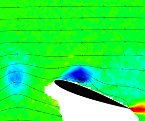
To understand the differences in the wake–wing interactions when the wing is located at the wake centreline and the optimal location, we examined instantaneous flow fields. Figure 8 presents three representative instantaneous vorticity fields for  ${y_{LE}}/c = 0$ in figure 8(a), and three images for the optimal location
  ${y_{LE}}/c ={-} 0.6$ in figure 8(b), at α = 20° and
  ${x_{LE}}/c = 2.0$ for the H/c = 0.5 wake generator. The comparison of the images in figures 8(a) and 8(b) suggests that, at the wake centreline, the flow fields are widely varying from fully attached (left), with a LEV above mid-chord (middle) to fully stalled with wide wake (right). This is consistent with the large variations in the effective angle of attack at the wake centreline. The root-mean-square wake angle for this case is more than 20° (see figure 6b), which suggests that the sum of the wake angle and the geometric angle of attack (α = 20° in this case) varies from nearly zero or negative angles of attack to large angles of attack exceeding 40°. As a result, the wing experiences periods of attached and separated flows, and LEV formation in between them. In contrast, for the optimal case in figure 8(b), the flow is always separated at the leading edge, followed by the formation of a large LEV and separation bubble with reattachment further downstream, resulting in much higher time-averaged lift. This is also consistent with the smaller variations in the effective angle of attack (the root mean square of the wake angle is less than 5° in figure 6b), resulting in always separated flow at the leading edge and the LEV formation during the effective ‘pitch up’.

Figure 8. Instantaneous vorticity contours for α=20°,  ${x_{LE}}/c = 2.0$, H/c = 0.5: (a)
  ${y_{LE}}/c = 0$ and (b)
  ${y_{LE}}/c ={-} 0.6$.
3.4. Characteristics of LEVs
For α = 20°,  ${x_{LE}}/c = 2$ and H/c = 0.5, figures 9 and 10 present the phase-averaged vorticity contours for the wing at the wake centreline and at the optimal location, respectively. When the wing is located at the wake centreline, the birth of the clockwise LEV can be first noticed at t/T = 0.5, and its growth is visible until around t/T = 0.875. (The normalized time in the cycle is related to the phase angle in (2.2).) Subsequently, at t/T = 0, there is the first sign of the LEV shedding and then convecting at all later times, while weakening as the vortex becomes presumably more three-dimensional. Meanwhile, the incident vortex of the wake, which appears with small magnitude of vorticity, approaches and impinges on the wing (t/T = 0.25 and 0.375), with further loss of coherency. (The counter-clockwise vortex of the wake can be seen just near the leading edge at t/T = 0.75.) In contrast, the LEVs at the corresponding times are all larger for the optimal wing location in figure 10. Because of their large size, at some instants (t/T = 0.375 and 0.5) it is somewhat difficult to define a boundary to separate two successive LEVs. We note that, at t/T = 0.125, the separation bubble reattaches at the trailing edge. There was no direct impingement of the incident vortices, therefore, the vortex street retained its coherency with less dissipation throughout the cycle.

Figure 9. Phase-averaged vorticity superimposed with streamlines for α=20°,  ${x_{LE}}/c = 2.0,{y_{LE}}/c = \; 0$, H/c = 0.5.

Figure 10. Phase-averaged vorticity superimposed with streamlines for α=20°,  ${x_{LE}}/c = 2.0,{y_{LE}}/c = \; - 0.6$, H/c = 0.5.
Using the selected boundaries shown with dashed lines in figures 9 and 10, we calculated the circulation of the LEVs. The calculation of the circulation becomes more difficult for smaller H/c. As the thickness of the wake generator decreases, the frequency of the wake vortex street increases and their wavelength decreases. This makes the clear identification of the two neighbouring LEVs more difficult. Figure 11 illustrates this for H/c = 0.2. When the wing is located at the wake centreline (see figure 11a), it is still possible to identify individual LEVs (although with some subjectivity) and calculate the circulation by using the control volume A. However, when the wing is located at the optimal location (see figure 11b), it is impossible to identify the individual LEVs. In this case, we choose the control volume B to calculate the circulation over the suction surface of the wing as we cannot separate individual LEVs.

Figure 11. Illustration of the two control volumes for circulation computation, α=20°, H/c = 0.2, at (a)  ${y_{LE}}/c = 0$ and (b) at
  ${y_{LE}}/c = \textrm{optimal}\;\textrm{location}$.
For the even smaller value of H/c = 0.1, it is not possible to identify the individual vortices for both locations of the wing, and we calculated the circulation for the control volume B and present it in figure 12(a). The mean values for the optimal location and the wake centreline are close. It appears that the variations of the circulation for the control volume B approach the normalized circulation of the shear layer of the wing in freestream, which was measured as −1.25. The results for the other wake generators shown in figure 12 reveal that the difference between the mean values of the circulation for the two wing locations increases with increasing H/c (decreasing frequency and increasing LEV size). The maximum circulation of the LEVs for the optimal wing location also increases with increasing H/c. The maximum circulation of the LEVs for the optimal wing location can become nearly twice that of the case of the wing at the wake centreline. It is clear that the vorticity flux must be much larger for the optimal case even though the velocity fluctuations are smaller and the period of the flow oscillations is the same for both locations of the wing. It is interesting to note that the root-mean-square value of the cross-stream velocity fluctuations in the incident wakes at the optimal locations is small and does not vary much with H/c (see figure 6b). We note that whereas there is continuous vorticity shedding from the leading edge for the optimal case, the vorticity shedding from the leading edge does not occur during the attached flow phases when the wing is located at the wake centreline. Therefore, we conclude that, in an analogy with the effective angle of attack variations, the strongest LEV circulation and maximum time-averaged lift are achieved when operating in post-stall conditions throughout the cycle (always separated flows) with no reattachment at the leading edge.

Figure 12. Time history of normalised LEV circulation for α=20°,  ${x_{LE}}/c = 2.0$, (a) H/c = 0.1, (b) H/c = 0.2, (c) H/c = 0.3, (d) H/c = 0.4 and (e) H/c = 0.5.
The state of the flow (separated versus attached) can be detected by monitoring the local flow angle,  ${\tan ^{ - 1}}(\langle v\rangle /\langle u\rangle )$, near the leading edge at a location C (see the inset in figure 13). This particular location was chosen as it is sufficiently away from the surface (where the measurements are impossible), yet not too far away, and the surface slope at the closest location on the wing looks nearly horizontal at α = 20°. A panel code (Alexander Reference Alexander2021) allowed us to obtain an estimate of the flow angle at location C for potential flow (fully attached flow) as around 3°. This attached flow condition is shown as horizontal lines in all plots where the flow angle at C is compared for the wing located at the wake centreline and at the optimal location. In addition, the local flow angle at C measured for the wing in steady freestream was measured as a little less than 20°, and also plotted as horizontal lines in figure 13. When the wing is located at the wake centreline, the flow angle at C exhibits strong dependency on the wake generator as the amplitude of the wake angle fluctuations in the incident wake is large. For H/c = 0.4 and 0.5, the flow angle at C reaches as low as that of the potential flow and as high as 32°–37° where the deep stall is anticipated. When the wing is located at the optimal location, the flow angle at C has small amplitude oscillations around a mean which is slightly larger than that of the steady freestream, confirming that the flow is always separated at the leading edge for all wake generators. However, the amplitude of the small oscillations of the flow angle decreases for lower values of H/c, and correspondingly the time-averaged lift is smaller.

Figure 13. Local flow angle sampled at 0.05c above and downstream of leading edge for α = 20°,  ${x_{LE}}/c = 2.0$, at the wake centreline and optimal location, (a) H/c = 0.1, (b) H/c = 0.2, (c) H/c = 0.3, (d) H/c = 0.4 and (e) H/c = 0.5.
3.5. Discussion
So far, we have established that the time-averaged lift acting on the wing in the wake is larger than that in freestream, when the wing is set at a post-stall angle of attack. This is due to the formation and convection of LEVs due to the wake velocity fluctuations. There are similarities with unsteady aerodynamics of ‘dynamic stall’ of pithing or plunging wings (Ekaterinaris & Platzer Reference Ekaterinaris and Platzer1998). In the cases of unsteady freestream (Gursul & Ho Reference Gursul and Ho1992; Gursul, Lin & Ho Reference Gursul, Lin and Ho1994; Choi, Colonius & Williams Reference Choi, Colonius and Williams2015), the most effective frequency that provides maximum time-averaged lift in the post-stall regime corresponds to a wavelength that is around the chord length. For plunging airfoils (Cleaver et al. Reference Cleaver, Wang, Gursul and Visbal2011; Choi et al. Reference Choi, Colonius and Williams2015), the maximum time-averaged lift is produced at optimal frequencies on the order of fc/U∞ = O(1), corresponding to the optimal wavelengths on the order of the chord length.
For the post-stall flow control on an airfoil, Wu et al. (Reference Wu, Lu, Denny, Fan and Wu1998) found that periodic blowing–suction near the leading edge was the most effective when the excitation was at the subharmonic or higher harmonics of the natural wake instability. The importance of the subharmonic and the fundamental wake frequency in producing maximum time-averaged lift was also reported for small-amplitude airfoil oscillations (Cleaver et al. Reference Cleaver, Wang, Gursul and Visbal2011). It is known that the fundamental wake (natural vortex shedding) frequency is little affected by the wing aspect ratio, and falls in the range of  $fc\sin \alpha /{U_\infty } = 0.17\text{--} 0.19$ (Rojratsirikul et al. Reference Rojratsirikul, Genc, Wang and Gursul2011). In our experiments in the wake, the modified Strouhal number at α = 20° falls in the range of
  $fc\sin \alpha /{U_\infty } = 0.18\text{--} 0.96$ (the lowest value corresponding to H/c = 0.5).
The enhanced time-averaged lift of the wing in the wake has also a similar mechanism and frequency range to those of the active flow control methods applied for the separated flows over lifting surfaces (Greenblatt & Wygnanski Reference Greenblatt and Wygnanski2000). For a variety of wing flows, the active flow control research suggests that the optimal range is fc  $/$U∞ = 0.5–1.0, which compares well with the frequency range of the wakes in our experiments (see figure 5a). For H/c = 0.3, 0.4, and 0.5 (the three wakes generating large lift enhancement), the dimensionless frequency lies in the same range as 0.5–1.0, whereas the H/c = 0.5 case has fc
  $/$U∞ = 0.52. It is interesting to note that the most effective frequencies for oscillatory blowing to delay boundary-layer separation correspond to the creation of one to two vortices over the airfoil (Seifert et al. Reference Seifert, Bachar, Koss, Shepshelovich and Wygnanski1993; Seifert, Darabi & Wyganski Reference Seifert, Darabi and Wyganski1996).
Noting the similarities of the LEVs in our experiments with the dynamic stall vortices and flow control vortices induced by excitation, one expects that the size and the circulation of the LEVs should be directly correlated with the time-averaged lift enhancement. However, both oscillating wings and most methods of flow excitation at the leading edge for separation control are either two-dimensional or primarily two-dimensional. This is unlikely in our experiments in the turbulent wakes as discussed in the introduction. In order to examine the degree of two-dimensionality, we carried out crossflow measurements for incident wakes (in the absence of the downstream wing) at x/c = 2 (corresponding to the location of the leading edge of the wing when it is placed in the wake). Figure 14(a) shows the two-point cross-correlation coefficients of cross-stream velocity fluctuations Cvv using (3.1), where the reference location A is chosen as the wake centreline at the mid-span (y/c = 0, z/c = 2). The dashed lines outline the location and the thickness H of the wake generator. It is seen that the higher cross-correlation regions are roughly circular shapes with increasing radius as H/c is increased. Figure 14(b) presents the variation of the cross-correlation coefficient as a function of spanwise distance at y/c = 0. It is seen that the cross-correlation decays faster with spanwise distance with decreasing H/c. Using this information, we calculated the correlation integral scale L defined as
 \begin{equation}L/c = \int_{z/c = 0.5}^{z/c = 3.5} {{C_{vv}}\left( {\frac{y}{c} = 0,\frac{z}{c}} \right)\,\textrm{d}\left( {\frac{z}{c}} \right)} .\end{equation}
Alternatively, the spanwise length scale Ls is defined as the location at which the correlation coefficient drops by  ${e^{ - 1}}$ (Hayakawa & Hussain Reference Hayakawa and Hussain1989). Figure 14(c) shows the correlation integral scale and spanwise length scale as a function of H/c. The two length scales are relatively small in magnitude in comparison with the wingspan. It is seen that the correlation integral scale is roughly three times the thickness of the wake generator at this streamwise station and in this range of wake Reynolds numbers. This is the same order of magnitude reported for circular cylinder (Hayakawa & Hussain Reference Hayakawa and Hussain1989) and airfoil (Turhan et al. Reference Turhan, Wang and Gursul2022) wakes at similar wake Reynolds numbers. It is remarkable that, for H/c = 0.5, a maximum lift increase of 57 % of the lift in freestream is achieved with a correlation length scale of around 1.5c in the spanwise direction.

Figure 14. (a) Cross-correlation contours for all wake generators; (b) cross-correlation of cross-stream velocity as a function of spanwise distance; (c) correlation integral scale (L/c) and spanwise length scale (Ls/c) of the wake at x/c = 2.0 as a function of wake generator thickness.
With increasing H/c, the size and circulation of the LEVs as well as the spanwise correlation of the unsteady flow increase, resulting in the increase of the maximum lift coefficient. For example, when H/c is increased from 0.3 to 0.5, the maximum lift increment compared with freestream increases 8 % with respect to H/c = 0.3, whereas the maximum LEV circulation grows 35 % and the spanwise correlation length scale grows 55 %. The spanwise length scale grows faster, however, we cannot say which one of these parameters contributes more.
3.6. Effect of streamwise location of wing
We measured the variation of the time-averaged lift coefficient CL with angle of attack α at  ${x_{LE}}/c = 1,2,3,4$, and 5 for H/c = 0.5 when the wing is placed at the wake centreline, optimal offset location and in the freestream (not shown here). The decay of the mean streamwise velocity and the root mean square of the cross-stream velocity fluctuations in the streamwise direction of the incident wake is evident in figure 4. However, we found relatively weak effect on the time-averaged lift force for the range of
  ${x_{LE}}/c = 1\text{--} 5$. The maximum lift coefficient observed was at
  ${x_{LE}}/c = 3.0({C_{L,max}} \approx 0.98)$, which was 7 % higher than that observed at
  ${x_{LE}}/c = 2.0$. The other features, such as the existence of an optimal location at a non-zero offset distance at the edge of the wake and smaller initial lift slope at the wake centreline are similar to the previous observations. The initial lift slope increases monotonically with the increasing streamwise location of the wing.
In order to understand the initial increase and subsequent decay of the maximum lift coefficient, we carried out velocity measurements for  ${x_{LE}}/c = 2,3,4$. We present the variations of the circulation of the LEVs in figure 15. It is seen that the maximum LEV circulation is the largest at the intermediate streamwise location of
  ${x_{LE}}/c = 3$, which is in agreement with the largest time-averaged lift for this location. The phase-averaged vorticity fields with streamlines at the instant of the maximum circulation are also shown in figure 15. It is seen that all three flow fields have highly curved streamlines, but for the optimal location, there is reattachment of the flow near the trailing edge.

Figure 15. Time history of normalised LEV circulation (left column) and the phase-averaged vorticity contour at the instance with maximum LEV circulation (right column) for α=20°, H/c = 0.5, (a)  ${x_{LE}}/c = 2.0$, (b)
  ${x_{LE}}/c = 3.0$ and (c)
  ${x_{LE}}/c = 4.0$.
We also investigated the spanwise coherence of the flow for each streamwise location of the wing. The inset of figure 16 shows the schematic of the crossflow PIV measurements at the leading edge and the trailing edge of the wing. The cross-correlation contours (reference point is at the projection of the leading edge and mid-span) are shown in figure 16 for α = 20°,  ${x_{LE}}/c = 3.0$. The dashed lines indicate the projections of the leading edge and the trailing edge. At the leading edge, there is slightly smaller region of larger coherence at the optimal location in comparison with the wake centreline (compare with figure 14). However, after the flow separation near the leading edge, the coherence of the flow drops to similar levels at the trailing edge for both cases. We found little difference between the variations of the spanwise correlation for all three wing locations
  ${x_{LE}}/c = 2,3,4$. The optimal streamwise location appears to be determined by the circulation of the LEVs.

Figure 16. Cross-correlation of cross-stream velocity when the wing was placed at wake centreline and optimal location, α=20°,  ${x_{LE}}/c = 3.0$, at (a) leading edge and (b) trailing edge.
4. Conclusions
The unsteady aerodynamics of a stationary wing in turbulent wakes with varying scale and dominant frequency has been investigated experimentally. PIV and lift force measurements have been carried out with the main focus on the post-stall aerodynamics. The scale of the wakes was varied by using different wake generators and placing the wing at different streamwise locations. When the wing is in the wake, there may be some decrease in the time-averaged lift at pre-stall angles of attack compared with the freestream. This happens especially when the wing is subjected to the large velocity fluctuations near the wake centreline, however, the lift decrease vanishes as the wing is placed at larger offset distances from the wake centreline. In contrast, for post-stall angles of attack, there is generally an increase in the time-averaged lift compared with the freestream. There is an optimal offset distance (near the edge of the wake) at which the time-averaged lift becomes maximum while it is still possible to observe increased lift near the wake centreline. Maximum time-averaged lift coefficients can reach levels up to 64 % higher than that of the freestream case at an angle of attack of α = 20°, corresponding to the increases of 36 % in the maximum lift coefficient of the wing and 9° in the stall angle. At the optimal offset locations in the incident wakes, the mean streamwise velocity is nearly equal to the freestream velocity, and the amplitude of the cross-stream velocity fluctuations is much smaller than that at the centreline.
When the wing is placed at the wake centreline, instantaneous flow widely varies from fully attached to fully stalled. Whereas the wing experiences periods of attached and separated flows at the wake centreline, the flow is always separated at the leading edge for the optimal offset distance. In the latter case, we observe the formation of a large LEV and separation bubble with reattachment further downstream, resulting in much higher time-averaged lift. For the largest wavelength of the wake, the separation bubble covers the whole surface at some point in the cycle and the reattachment point reaches near the trailing edge. The maximum circulation of the LEVs for the optimal wing location can reach twice that of the wing at the wake centreline, which must be due to the larger vorticity flux even though the velocity fluctuations are smaller. This is attributed to continuous vorticity shedding from the leading edge for the optimal case, whereas the vorticity shedding from the leading edge is interrupted for the periods of attached flow when the wing is located at the wake centreline.
With increasing H/c (increasing wavelength and decreasing frequency of the wake), the maximum circulation of the LEVs for the optimal wing location increases, despite the magnitude of the velocity fluctuations remaining small and nearly the same. This implies that the stronger LEV and larger time-averaged lift are achieved when operating in the post-stall conditions throughout the cycle with longer periods. We note the similarities with wake synchronization (vortex lock-in) and resonance with the wake instabilities (fundamental and subharmonic of natural vortex shedding) as well as active flow control methods with periodic excitation of the separated flows. These observations suggest that time-averaged lift becomes maximum when the Strouhal number of the excitation frequencies are on the order of fc/U∞ = O(1), corresponding to the optimal wavelengths on the order of the chord length.
However, we also show that the degree of the two-dimensionality of the unsteady turbulent wakes is substantially smaller than that of nominally two-dimensional excitation. The spanwise length scale is on the order of the thickness of the wake generator. It increases linearly with the wake generator thickness for the incident wake; however, the LEV circulation also increases with increasing H/c. Hence, we cannot determine the relative contribution of the spanwise length scale. It does not vary much in the streamwise direction; therefore, the LEV circulation directly affects the time-averaged lift. The spanwise length scale decreases significantly during the interaction of the incident wake with the wing.
Funding
The authors would like to acknowledge the funding from the University of Bath PhD studentship for the first author and the Engineering and Physical Sciences Research Council (EPSRC) strategic equipment Grant (EP/K040391/1).
Declaration of interests
The authors report no conflict of interest.


