2.1. Jet velocity experiments

Following methods in Houghton & Dabiri (Reference Houghton and Dabiri2019), the fluid velocity induced by the aggregation was assessed with simultaneous volumetric animal number density and two-dimensional velocity measurements in a $0.5\ \textrm {m} \times 0.5\ \textrm {m} \times 1.2\ \textrm {m}$ tall, well-mixed tank.

Lights were utilized to control the animal motion, with an LED array pointing upward through the clear acrylic bottom of the tank and a single focused LED pointed vertically downward from the top of the tank (figure 1). Another focused LED was pointed horizontally just below the water surface intersecting the vertical beam in order to draw the animals to the edge of the tank after they reached the surface. The lower LED array was used to group the animals at the bottom of the tank initially, and the strong phototactic response of the swimmers resulted in a steady upward migration following activation of the upper LED and deactivation of the lower LED array (see supplementary movie available at https://doi.org/10.1017/jfm.2020.618). Experimental studies focused solely on the upward migrations.

Figure 1. Experimental set-up to measure jet velocity: (a) animals grouped at the bottom initially; (b) animals drawn to the surface, and then to the side, with a focused LED from above. A two-dimensional red laser sheet illuminates particles seeded in the flow.

Image analysis was used to measure the local animal number densities within the aggregation by obtaining the animal count within the known illuminated volume created by the focused LED. Local animal densities were of the same order of magnitude as reported values for oceanic swarms, which range from 10 000–450 000 animals m$^{-3}$ (Hamner et al. Reference Hamner, Hamner, Strand and Gilmer1983; O'Brien Reference O'Brien1988; Huntley & Zhou Reference Huntley and Zhou2004). Estimates of the animal swimming velocities were obtained using object centroid tracking and were averaged in one second bins.

To measure the fluid velocity within the aggregation, the experimental tank was seeded with $13\,\mathrm {\mu }\textrm {m}$ neutrally buoyant glass beads and illuminated with a two-dimensional red laser sheet. Pairs of subsequent frames (${\rm \Delta} T = 0.04\ \textrm {s}$) were used to conduct particle image velocimetry (PIV) using PIVLab (Thielicke & Stamhuis Reference Thielicke and Stamhuis2014). Vertical and horizontal velocities within the two-dimensional slice through the centre of the aggregation were obtained using a multi-pass method with two iterations and a decreasing window size from $64 \times 64$ pixels to $32 \times 32$ pixels and a 50 % overlap. Animals were masked out prior to processing, with the identical mask applied to the pair of processed images.

For full experimental details, including complete experimental tank conditions and image analysis methods, see Houghton & Dabiri (Reference Houghton and Dabiri2019).

2.2. Density-stratified experiments

Two experimental set-ups are presented in a density-stratified environment, one focused on transient dynamics in a linear stratification and one measuring irreversible mixing in a two-layer stratification. Transient dynamics within a linearly salt-stratified water column were studied in a $0.9\ \textrm {m} \times 0.9\ \textrm {m} \times 2\ \textrm {m}$ tall tank, with a buoyancy frequency of $N = 0.05\ \textrm {s}^{-1}$ to assess the importance of a restratifying force. Repeated control profiles were taken over the course of an hour prior to starting an experiment, and changes to the density stratification were negligible, indicating that thermal convection was not affecting the flow. Density was measured using a temperature-salinity probe (see the methods section of Houghton et al. Reference Houghton, Koseff, Monismith and Dabiri2018). A 1 W, 447 nm (blue) laser was used as the light stimulus rather than focused LEDs for increased illumination intensity over a larger height. Transient perturbations to the density stratification in the tank were measured as the animals swam upward toward the light using a vertically traversing density probe (Precision Measurement Engineering) located 5 cm horizontally from the centreline of the migration. Following each migration and measurement of the perturbations, the animals could be returned to the bottom of the tank by powering off the upper blue laser and powering on a lower green laser.

Long-term impacts to the density profile (i.e. mixing) were measured in the $0.5\ \textrm {m} \times 0.5\,\textrm {m} \times 1.2\,\textrm {m}$ tank. Animals were introduced at a tank averaged value of $46\,000\pm 5000\ \textrm {animals}\,\textrm {m}^{-3}$ to $138\,000\pm 5000\ \textrm {animals}\,\textrm {m}^{-3}$. These experiments used a two-layer stratification with buoyancy frequencies across the 0.2 m thick interface of $N = 0.04\text {--}0.13\ \textrm {s}^{-1}$. This corresponded to a salt concentration of 26.0 ppt in the upper mixed layer and 26.1–26.5 ppt in the lower mixed layer for the range of stratification strengths used. To simulate the passage of a swarm through a pycnocline, animal migrations were repeatedly induced over 120 min, switching the LED light stimulus between the top and bottom (upward and downward migration) every 10 min (figure 1). The long-term evolution of the initial two-layer stratification was measured with the same vertically traversing probe located 20 cm laterally from the migration. Density profiles were obtained every twenty minutes throughout a migration experiment, with repeated density profiles obtained at the end of a 120 min experiment to confirm that the tank was fully settled and horizontally homogeneous. For full density mixing experimental details, see Houghton et al. (Reference Houghton, Koseff, Monismith and Dabiri2018).

3.1. Governing equations

We employ the squirmer model introduced by Lighthill (Reference Lighthill1952) and adapted by Blake (Reference Blake1971) for Stokes flows to represent the swimmers. The squirmer model replaces the individual motion of numerous cilia around a spherical swimmer by a wave envelope and then evaluates the corresponding incompressible axisymmetric Stokes flow around the sphere. This model has been studied extensively and its usage has recently been extended to inertial finite Reynolds number flows, both analytically (Wang & Ardekani Reference Wang and Ardekani2012; Khair & Chisholm Reference Khair and Chisholm2014) and numerically (Li & Ardekani Reference Li and Ardekani2014; Wang & Ardekani Reference Wang and Ardekani2015; Chisholm et al. Reference Chisholm, Legendre, Lauga and Khair2016; Li et al. Reference Li, Ostace and Ardekani2016). The squirmer swimmer generates thrust by imposing a radial and tangential velocity at the surface of the sphere such that, in polar coordinates,

(3.1)\begin{gather} u_\rho(\rho=R,\theta)=\sum_{n=0}^{\infty}A_nP_n\cos{\theta}, \end{gather}

(3.2)\begin{gather}u_\theta(\rho=R,\theta)=\sum_{n=1}^{\infty}\frac{2}{n(n+1)}B_n\sin \theta P'_n\cos{\theta}, \end{gather}

where $\theta$ is the polar angle to the swimming direction, $R$ is the radius of the sphere, $A_n$ and $B_n$ are the $n\textrm {th}$ mode of the radial and tangential squirming velocity components, and $P_n$ and $P'_n$ are the $n\textrm {th}$ Legendre polynomial and its derivative, respectively. It is common to consider a reduced-order model by neglecting the radial velocity and only retaining the first two modes of the squirming motion, such that the surface velocity of a squirmer reduces to a tangential component, as shown in figure 2 (Chisholm et al. Reference Chisholm, Legendre, Lauga and Khair2016). In the reference frame of the moving object, this tangential velocity is given by

(3.3)\begin{equation} u_\theta(\rho=R,\theta)=B_1\sin\theta+B_2\sin\theta\cos\theta . \end{equation}

Figure 2. Sketch of the squirmer swimmer. Here $\boldsymbol {e}_s$ defines the swimming direction, $\boldsymbol {r}$ is the vector from the centre of the sphere to a point at its surface, where the tangential velocity $u_\theta$ is imposed in the direction of $\boldsymbol {e}_\theta$, and $\theta$ denotes the angle between $\boldsymbol {r}$ and the swimming direction $\boldsymbol {e}_s$.

The amplitude $B_1$ of the first mode is responsible for propulsion, while that of the second mode $B_2$ accounts for the stress field generated by the swimmer (Blake Reference Blake1971). This reduced-order model for the squirmer, which only considers the first two modes, is sufficient to explore a variety of swimming mechanisms that produce very different flow patterns in the near and far field, in a wide range of inertial regimes (Chisholm et al. Reference Chisholm, Legendre, Lauga and Khair2016). Physically, the first term on the right-hand side of (3.3) is solely responsible for propulsion. The second coefficient, B2, determines the intensity of the stresslet exerted by the swimmer. In a Stokes flow, the terminal velocity $U=\frac {2}{3}B_1$ reached by a single squirmer is independent of $B_2$. The ratio $\beta =B_2/B_1$ determines the squirming mode, i.e. how thrust is generated by the squirmer. Squirmers with $\beta >0$ are defined as pullers, while those with $\beta <0$ are pushers. A puller generates thrust by accelerating fluid backwards in front of its body, while a pusher accomplishes the same by accelerating fluid behind its body, as shown in figure 3. The resulting effect on the fluid velocity field and on the transport of a diffusing scalar field varies with the magnitude of $\beta$ and with the Reynolds and Péclet numbers. Figure 4 illustrates the qualitative influence of the swimming mode on the flow field and on the concentration contours of a passive scalar field for $Re=20$ and $\beta =-3,0,3$. At this Reynolds number the recirculation region typically present above a pusher is quite thin. The streamline pattern associated with the neutral swimmer is fairly symmetric, while the puller gives rise to a pronounced recirculation region in its near wake. The velocity field corresponding to the swimming mode directly affects the transport of a passive scalar. While a pusher tends to carry along resident fluid near its front stagnation point, a puller drags along fluid in its near wake.

Figure 3. Axisymmetric surface velocity vectors in the reference frame of the squirmer for a pusher, neutral swimmer and puller.

Figure 4. Axisymmetric flow due to an inertial squirmer swimming across a passive scalar gradient at $Re=20$ for $\beta =-3$ (a,d), $\beta =0$ (b,e) and $\beta =3$ (c,f). The streamlines and velocity magnitude field in the reference frame of the swimmers (a–c), along with the concentration field and contour lines (d–f), illustrate the differences among the swimming modes.

To simulate the flow field associated with a swarm of squirmers, we solve the three-dimensional incompressible Navier–Stokes equations in the Boussinesq limit, in conjunction with an advection-diffusion equation for the density field. In addition, the conservation equations of linear and angular momentum are solved for each squirmer. We account for the effect of the squirmers on the fluid via the IBM (Mittal & Iaccarino Reference Mittal and Iaccarino2005; Biegert, Vowinckel & Meiburg Reference Biegert, Vowinckel and Meiburg2017). This approach adds a forcing term $\boldsymbol {f}$ to the momentum equation in order to enforce boundary condition (3.3) at the surface of the squirmer. The dimensional governing equations for the fluid motion and scalar transport in conservative form hence take the form

(3.4)\begin{gather} \boldsymbol{\nabla}\boldsymbol{\cdot} {\boldsymbol{u}} = 0 , \end{gather}

(3.5)\begin{gather}\frac{\partial{\boldsymbol{u}}}{\partial t}+\boldsymbol{\nabla}\boldsymbol{\cdot} \left(\boldsymbol{uu}\right)=-\frac{1}{\rho_f}\boldsymbol{\nabla} p + \nu{\rm \Delta} {\boldsymbol{u}} + \xi_f(\boldsymbol{x}) c \alpha\boldsymbol{g}+ {\boldsymbol{f}} , \end{gather}

(3.6)\begin{gather}\frac{\partial c}{\partial t}+\boldsymbol{\nabla}\boldsymbol{\cdot}\left({\hat{\boldsymbol{u}}} c\right) = \boldsymbol{\nabla} (\kappa \boldsymbol{\nabla} c ) , \end{gather}

where $\boldsymbol {u}$ represents the fluid velocity in Cartesian coordinates, $p$ indicates the pressure and $\nu$ is the constant kinematic viscosity. As a reference density $\rho _f$, we choose the value $1000\ \textrm {kg}\,\textrm {m}^{-3}$, and $\alpha$ denotes the expansion coefficient associated with the concentration field $c$. The gravity term of (3.5) was derived by assuming a linear relationship between the local density and the scalar concentration

(3.7)\begin{equation} \rho =\rho_f(1+ \alpha c). \end{equation}

Here $\kappa$ represents the scalar diffusivity, and $\hat {\boldsymbol {u}}$ is the compound velocity defined as the fluid velocity inside the fluid domain and the particle velocity within each particle, i.e. the solid body motion of the rotating and translating swimmer (see appendix A). This ensures that there is no advective transport of concentration within the sphere due to the IBM solution to the fluid equations. Here $\boldsymbol{\xi} _f(\boldsymbol{x})$ denotes the indicator function of the fluid phase,

(3.8)\begin{equation} \xi_f(\boldsymbol{x}) =\begin{cases} 1 & \text{if}\ \boldsymbol{x} \in \varOmega_f,\\ 0 & \text{if}\ \boldsymbol{x} \in \varOmega_p, \end{cases} \end{equation}

where $\varOmega _f$ and $\varOmega _p$ indicate the volumes occupied by the fluid and particle phases, respectively. The governing equations are solved inside the numerical domain $\varOmega = \varOmega _f \bigcup \varOmega _p = [0 , L_x] \times [0, L_y] \times [0 , L_z]$ with edge lengths $L_x,L_y, L_y$, where $x$ and $z$ denote the horizontal directions and $y$ points in the upward vertical direction of swimming.

In order to track the concentration field as it is convected and diffused within the fluid, without crossing into the swimmers, we employ the VoF approach (Ardekani et al. Reference Ardekani, Asmar, Picano and Brandt2018). Within this VoF framework, the diffusivity $\kappa$ takes the constant value $\kappa _f$ in the fluid phase and the constant value $\kappa _p=0$ in the particle phase. We represent the tangential velocity discontinuity at the surface of the swimmers by a smoothing function to transition from fluid to particle velocity over a thickness of one grid cell ${\rm \Delta} x$ (see appendix A). Physically, this transition layer represents the boundary layer from the tip of the cilia to the ciliated edge of the swimmer. We impose a no-flux condition at the true swimmer surface, so that scalar concentration trapped in the thin modelled ciliated region is able to diffuse into the fluid. Leakage of scalar concentration from within the swimmer's body is minimized by refining the grid, and mass transfer across the surface of the swimmers was negligible over simulation times considered.

The particle motion is governed by the conservation of linear and angular momentum

(3.9)\begin{gather} m_p\frac{\textrm{d}{\boldsymbol{u}}_p}{\textrm{d}t}=\int_{\varGamma_p}{\boldsymbol{\tau}} \boldsymbol{\cdot} {\boldsymbol{n}}\,\textrm{d}A-V_p\left(\rho_p-\rho_f\right) \boldsymbol{g} +{\boldsymbol{F}}_c, \end{gather}

(3.10)\begin{gather}I_p\frac{\textrm{d}{\boldsymbol{\omega}}_p}{\textrm{d}t}=\int_{\varGamma_p} {\boldsymbol{r}}\times\left({\boldsymbol{\tau}}\boldsymbol{\cdot}{\boldsymbol{n}}\right)\textrm{d}A+ {\boldsymbol{T}}_c, \end{gather}

where $m_p$, $I_p$, $V_p$ and $\rho _p$ are the mass, moment of inertia, volume and density of the particle. The hydrodynamic stress tensor $\tau = -p\boldsymbol {I} + \rho _f\nu [\boldsymbol {\nabla } \boldsymbol {u} + (\boldsymbol {\nabla }\boldsymbol {u})^\textrm {T}]$ is projected onto the outward surface normal vector $\boldsymbol {n}$ along the particle surface $\varGamma _p$. The terms $\boldsymbol {F}_c$ and $\boldsymbol {T}_c$ account for collision forces during particle-particle or particle-wall interactions. Normal collision forces are evaluated from a simple linear spring-dashpot model, while tangential collision forces are neglected. Overlap between swimmers is avoided following a method similar to the one described in Li et al. (Reference Li, Ostace and Ardekani2016), in which the repulsive force is applied when the swimmers come within two grid sizes ${\rm \Delta} x$ of each other. A detailed description of the fluid solver and collision model, along with corresponding validation information, is provided in Biegert et al. (Reference Biegert, Vowinckel and Meiburg2017).

In the classical form of the IBM, the forcing term $\boldsymbol {f}$ accounts for the no-slip condition at the surface $\varGamma _p$ of a particle by enforcing the condition

(3.11)\begin{equation} \boldsymbol{u}=\boldsymbol{u}_p+\boldsymbol{\omega}_p \times \boldsymbol{r}\quad \text{on}\ \varGamma_p, \end{equation}

where $\boldsymbol {u}_p$ and $\boldsymbol {\omega }_p$ denote the translational and angular velocities of the particle, respectively, and $\boldsymbol {r}$ indicates the position vector from the centre of the particle to a point on its surface. For the present squirmer simulations, this traditional form of the IBM is modified, and the forcing term $ \boldsymbol{f} $ is instead calculated such as to impose the relative squirming velocity at the Lagrangian marker points on the particle surface

(3.12)\begin{equation} \boldsymbol{u}=\boldsymbol{u}_p+\boldsymbol{\omega}_p\times \boldsymbol{r}+u_\theta\boldsymbol{e}_\theta\quad \text{on}\ \varGamma_p, \end{equation}

where $u_\theta \boldsymbol {e}_\theta$ is the squirmer slip velocity imposed at the marker point, acting in the direction of the coordinate vector $\boldsymbol {e}_\theta$.

3.2. Non-dimensional formulation

The equations are rendered dimensionless by employing the swimmer radius $R$ and the terminal velocity of a squirmer in the Stokes regime, $\frac {2}{3}B_1$ (Blake Reference Blake1971), as characteristic length and velocity scales, respectively. For all simulations, the characteristic concentration $C$ is chosen such that the dimensionless concentration varies between 0 and 1. The non-dimensional variables are thus given by

\begin{align*} & \boldsymbol{x}\to R{\boldsymbol{x}'},\quad \boldsymbol{u} \to \frac{2}{3}B_1 {\boldsymbol{u}}',\\ & t\to \frac{3R}{2B_1}t',\quad p\to \rho_f \left(\frac{2}{3}B_1\right)^2p',\\ & c\to C c', \quad F_c\to \rho_f \left(\frac{2}{3}B_1\right)^2R^2 F_c',\\ & T_c\to \rho_f \left(\frac{2}{3}B_1R\right)^2R^3 T_c. \end{align*}

Dropping the prime, the dimensionless governing equations become

(3.13)\begin{gather} \boldsymbol{\nabla}\boldsymbol{\cdot} {\boldsymbol{u}} = 0, \end{gather}

(3.14)\begin{gather}\frac{\partial{\boldsymbol{u}}}{\partial t}+\boldsymbol{\nabla}\boldsymbol{\cdot} \left(\boldsymbol{uu}\right)=-\boldsymbol{\nabla} p + \frac{1}{Re}{\rm \Delta} {\boldsymbol{u}} +Ri\boldsymbol{\xi}_f{\boldsymbol{e}}_gc+ {\boldsymbol{f}}, \end{gather}

(3.15)\begin{gather}\frac{\partial c}{\partial t}+\boldsymbol{\nabla}\boldsymbol{\cdot}\left({\boldsymbol{u}}c \right) = \frac{1}{Pe}{\rm \Delta} c, \end{gather}

where $Re=\frac {2}{3}({B_1R}/{\nu })$, $Ri=g C \alpha R/\rho _f(2/3B_1)^2$, $Pe=\frac {2}{3}({B_1R}/{\kappa _f})$. Additionally, a reference density variation is defined as ${\rm \Delta} \rho = C \alpha$. The particle momentum equations become

(3.16)\begin{gather} \hat\rho_p V_p \frac{\textrm{d}{\boldsymbol{u}}_p}{\textrm{d}t}= \frac{1}{Re}\int_{\varGamma_p}{\boldsymbol{\tau}}\boldsymbol{\cdot} {\boldsymbol{n}}\,\textrm{d}A- V_p\left( \hat \rho_p-1\right) \hat{\boldsymbol{g}}+{\boldsymbol{F}}_c, \end{gather}

(3.17)\begin{gather}I_p\frac{\textrm{d}{\boldsymbol{\omega}}_p}{\textrm{d}t}=\frac{1}{Re} \int_{\varGamma_p}{\boldsymbol{r}}\times\left({\boldsymbol{\tau}} \boldsymbol{\cdot}{\boldsymbol{n}}\right)\textrm{d}A+{\boldsymbol{T}}_c, \end{gather}

with $\hat {\boldsymbol {g}}=\boldsymbol {g}R/(\frac {2}{3}B_1)^2$, $\hat \rho _p=\rho _p/\rho _f$, $V_p = \frac {4}{3}{{\rm \pi} }$ and $I_p = \frac {8}{15}{\rm \pi}$. The non-dimensional squirmer velocity boundary condition becomes $u_\theta = \frac {3}{2}(\sin \theta + \beta \sin \theta \cos \theta )$.

3.3. Active control of swimming direction

The phototactic response of the brine shrimp drives the vertical migration of the swarm, which in turn leads to the formation of a large-scale jet and the associated irreversible mixing (Houghton et al. Reference Houghton, Koseff, Monismith and Dabiri2018). To reproduce this scenario in our simulations, we model the shrimp's phototactic response by modifying the squirming velocity in order to actively control the orientation of the swimmer. This is accomplished by imposing a stronger velocity on the side of the swimmer that is oriented away from the target than on the side facing the target, so that the squirmer rotates towards the target. We take the velocity non-symmetry to be proportional to the misalignment $\theta _t$ between the swimming and target directions, as shown in figure 5, so that

(3.18)\begin{equation} \cos{\theta_t}=\boldsymbol{e}_{\boldsymbol{s}}\boldsymbol{\cdot}\boldsymbol{e}_{\boldsymbol{t}}. \end{equation}

Locally, the value of the velocity modulation at a given point on the surface of the spherical swimmer further depends on the angle $\phi$ between the projection of the position vector $\boldsymbol {r}$ and the projection of the target vector $\boldsymbol {e}_{\boldsymbol {t}}$ onto the plane normal to $\boldsymbol {e}_{\boldsymbol {s}}$. This angle is given by

(3.19)\begin{equation} \cos{\phi}=\frac{\tilde{\boldsymbol{r}}\boldsymbol{\cdot}\tilde{\boldsymbol{e}}_{\boldsymbol{t}}} {||\tilde{\boldsymbol{r}}||\boldsymbol{\cdot}||\tilde{\boldsymbol{e}}_{\boldsymbol{t}}||}, \end{equation}

where $\tilde {\boldsymbol {r}}$ and $\tilde {\boldsymbol {e}}_{\boldsymbol {t}}$ are defined as

(3.20a–b)\begin{equation} \tilde{\boldsymbol{r}}=\boldsymbol{r}-(\boldsymbol{r}\boldsymbol{\cdot}\boldsymbol{e}_{\boldsymbol{s}}) \boldsymbol{e}_{\boldsymbol{s}}\quad \text{and}\quad \tilde{\boldsymbol{e}}_{\boldsymbol{t}}=\boldsymbol{e}_{\boldsymbol{t}}-( \boldsymbol{e}_{\boldsymbol{t}}\boldsymbol{\cdot}\boldsymbol{e}_{\boldsymbol{s}}) \boldsymbol{e}_{\boldsymbol{s}}. \end{equation}

We introduce a modulation function

(3.21)\begin{equation} G(\theta_t,\phi)=\sqrt{1-A(\theta_t)\cos(\phi)} , \end{equation}

where $A(\theta _t)$ controls the magnitude of the asymmetry and is such that $0<A<1$. We propose to evaluate $A$ as

(3.22)\begin{equation} A_{q,\gamma}=q+(1-q) \textrm{erf}\left(\gamma \left(1-\cos\theta_t\right)\right) . \end{equation}

The amplitude of the asymmetry using this model jumps to the step value $q$ as soon as a non-negligible misalignment is measured, and it smoothly increases to unity using an error function. We use $\gamma$ to modulate how sharply the swimmer will transition from a weak correction to a strong correction of its swimming direction, depending on the value of $\theta _t$. The phototaxis model is heuristic and based on qualitative observations of the response of the A. salina to light in the laboratory environment. In the IBM implementation of the squirmer model the motion of the particle is a result of fluid forces induced by the velocity difference imposed at the surface of the particle. In order to stay consistent with this formalism, we do not impose an external torque (as can, for instance, be used to study of the effect of gyrotaxis on plankton migration; see Mitchell, Okubo & Fuhrman (Reference Mitchell, Okubo and Fuhrman1990)) to the equation of motion of the particles, but instead choose to modify the surface velocity difference. Both approaches succeed in effectively adapting the swimming direction to external stimuli. The parameters of the model were chosen such that a single swimmer would correct its misalignment with a target within a few body lengths, but were found to have a negligible impact on the simulations presented in the following. Finally, the asymmetric squirming velocity is given by

(3.23)\begin{equation} u_\theta=F(\theta)\cdot G(\theta_t,\phi) , \end{equation}

where $F(\theta )=B_1\sin \theta + B_2\sin \theta \cos \theta$ is the original squirming velocity.

Figure 5. Sketch of an active squirmer with phototactic response. The misalignment $\theta _t$ is the angle between the swimming direction $\boldsymbol {e}_{\boldsymbol {s}}$ and the desired target direction $\boldsymbol {e}_{\boldsymbol {t}}$. $\phi$ is the angle between the projection of $\tilde {\boldsymbol {r}}$ and the projection of $\tilde {\boldsymbol {e}}_{\boldsymbol {t}}$ onto the plane normal to the swimming direction $\boldsymbol {e}_{\boldsymbol {s}}$.

3.4. Numerical set-up

The simulations are conducted with our in-house code PARTIES, a second-order accurate finite difference solver based on a staggered uniform Cartesian grid (Biegert et al. Reference Biegert, Vowinckel and Meiburg2017). Time integration is performed by a low-storage, third-order Runge–Kutta method, based on a pressure-projection approach for satisfying the continuity constraint. The volume fraction of the swimmers in the simulations is chosen to mimic the animal number density of the experiments. The appropriate fluid velocity and concentration field boundary conditions at the surface of the swimmers are enforced via the IBM and VoF techniques, as described above. The above simulation approach allows us to consider a variety of flows for different boundary and initial conditions.

The governing parameters are chosen to closely match the experimental values. As described in § 4, the typical animal velocity observed in the experiments is $1\ \textrm {cm}\,\textrm {s}^{-1}$. We base the size of the spherical squirmer on the length of the A. salina appendages of order 1 cm, which also represents the characteristic length scale over which the fluid is being accelerated. Hence, we select as the squirmer radius $R=0.5\ \textrm {cm}$. For a fluid viscosity of $10^{-6}\ \textrm {m}^2\,\textrm {s}^{-1}$, this yields a Reynolds number $Re=50$, which fits within the range of inertial flows recently investigated using the squirmer model (Chisholm et al. Reference Chisholm, Legendre, Lauga and Khair2016; Li et al. Reference Li, Ostace and Ardekani2016). Wilhelmus & Dabiri (Reference Wilhelmus and Dabiri2014) presented PIV measurements of the near-body flow field surrounding a single A. salina and showed that the dominant flow feature consisted of a quasi-steady downward jet in which the vertical velocity reached values of $5\ \textrm {mm}\,\textrm {s}^{-1}$. Numerical simulations of a single squirmer swimmer at $Re=50$ and $\beta =-3$ (see figure 6 of a slice of the vertical velocity) show that while very near-field dynamics are dominated by the tangential velocity imposed at the body, near- and far-field dynamics are dominated by a single, steady vertical jet. The vertical velocity within the jet reaches values identical to those measures by Wilhelmus & Dabiri (Reference Wilhelmus and Dabiri2014), which indicates that the parameter choice of $Re=50$ and $\beta =-3$ capture the dominant jet feature of the A. salina.

Figure 6. Slice in the vertical plane of the vertical velocity $v$ through the centre of a single squirmer swimmer at $Re=50$ and $\beta =-3$, with quiver plot of plane velocity field superimposed. The vertical velocity away from the swimmer is dominated by a downward jet reaching dimensional velocities of $0.5\ \textrm {cm}\,\textrm {s}^{-1}$, comparing well to the PIV measurements of Wilhelmus & Dabiri (Reference Wilhelmus and Dabiri2014).

4.1. Experimental observations

A. salina exhibit slight negative buoyancy, similar to most marine zooplankton (Pond Reference Pond2012), and, therefore, must overcome both gravity and fluid drag to propel themselves upward. The required thrust for this upward swimming is produced via the rearward propulsion of fluid by the metachronal beating of the animal appendages (Wilhelmus & Dabiri Reference Wilhelmus and Dabiri2014), similar to the swimming modes of many marine zooplankton such as Antarctic and Pacific krill (Catton et al. Reference Catton, Webster, Kawaguchi and Yen2011).

In the laboratory migrations, as the animal number density within the aggregation increased, the distance between each swimmer decreased and the fluid wakes of individual swimmers began to interact, as seen in figure 7. Previous work found that the individual flow fields combined to form a coherent downward jet-like flow within the aggregation, even in the presence of strong stratification relative to oceanic values (Houghton et al. Reference Houghton, Koseff, Monismith and Dabiri2018). Here, we present the dependence of the jet-like flow on animal number density.

Figure 7. Experimental measurements. Upper row: Pseudo-colour plot of instantaneous vertical velocity in the illuminated plane at three different times. Lower row: Zoom of region with in-plane velocity vectors at three different times: (a) $t = 16.4\ \textrm {s}$, (b) $t = 56.4\ \textrm {s}$ and (c) $t = 100\ \textrm {s}$.

During the laboratory migrations conducted, following activation of the upper focused LED, animal number density within the field of view gradually increased over the first 80–100 s. At first, fluid motion within the illuminated plane was limited to individual wakes visualized due to animals swimming in the laser sheet. Over time, animal number density asymptoted and a spatially coherent downward flow developed (see figure 8). The initially high normalized spatial standard deviation of the vertical fluid velocity decreased as the coherent downward jet developed within the swarm. The period from 100–155 s was used for asymptotic values, chosen for the relatively constant animal number densities among all experiments. To obtain an average asymptotic fluid velocity, all vertical velocity values within the field of view between 100–155 s were averaged. As would be expected, migrations with a higher asymptotic animal number density resulted in a larger asymptotic downward jet velocity (see figure 9). Each animal produced thrust in the form of a downward induced velocity in order to propel itself up against gravity and drag. Thus, the momentum in the flow and large-scale jet velocity increased with increasing animal number density.

Figure 8. Experimental measurements. (a) Instantaneous animal count in the field of view, in 1 s bins. (b) Average animal swimming speed over time, in 1 s bins. Coloured lines from dark to light correspond to the first experiment to the last experiment run. Animal count within the migration decreased over time, either due to reduced phototaxis or overall endurance. Animal velocities were higher at early times, either because they were naturally faster or did not have to contend with the flow fields of preceding animals.

Figure 9. Experimental measurements: (a) average vertical fluid velocity during each migration over time; (b) asymptotic jet velocity as a function of animal number density. Error bars represent the standard deviation of the animal count (horizontal) and fluid velocity (vertical). The standard deviation of the animal count is due to animal density variability during the asymptotic period as well as large noise in the counting algorithm. Adapted from Houghton & Dabiri (Reference Houghton and Dabiri2019).

4.2. Discrete swimmer simulations

We employ numerical simulations in order to investigate the formation of a jet by a homogeneous swarm of squirmers moving in a constant density fluid for various animal number densities. Towards this end, we consider a group of neutrally buoyant swimmers that are initially distributed randomly in fluid at rest. We apply periodic conditions in the swimming direction $y$ and the spanwise $z$-direction, so that the swimmers can exit the computational domain at one boundary and re-enter it at the opposite one (figure 10). Slip walls are employed in the spanwise $x$-direction. The volume fraction of the swimmers is determined by their number and the size of the simulation domain. All simulations have $Re=50$ and $\beta =-3$, and they employ a domain size of $20\times 40\times 10$ with a constant grid spacing of $1/30$. The size of the computational domain in the $z$-direction being limited to 10 swimmer radii, we note that the periodicity imposed in this direction might affect the flow field and that the exact quantitative value of the measured mixing might be different for larger, more realistic domains. We also note that the domain size is consistent with previous numerical studies that considered biogenic mixing in periodic domains (see, for instance, Wang & Ardekani Reference Wang and Ardekani2015). The target light source is placed at height $2L_y$, centred in the horizontal plane, so that the swimmers move upwards. We conducted four simulations with 47, 94, 187 and 373 neutrally buoyant swimmers, corresponding to volume fractions of 2.46 %, 4.92 %, 9.79 % and 19.53 %, in order to closely match experimental conditions, as well as estimates of the packing density in the ocean (Huntley & Zhou Reference Huntley and Zhou2004; Wang & Ardekani Reference Wang and Ardekani2015).

Figure 10. Numerical set-up for simulating the formation of a jet by a homogeneous swarm of swimmers in a periodic domain.

As the swimmers move through the domain and interact, they influence each other's velocity and direction. Figure 11 shows a two-dimensional slice of a typical configuration, along with the fluid velocity vectors and contours of the velocity magnitude. The figure demonstrates that the hydrodynamic interactions among the swimmers occur both at the scale of the swimmers themselves, but also at scales several times larger than the swimmer size due to the substantial extent of their wakes.

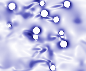
Figure 11. Discrete swimmer simulation of the jet formation with a volume fraction of swimmers of $9.79\,\%$. (a) Pseudo-colour plot of the vertical velocity in a slice of the three-dimensional domain. (b) Zoomed-in view corresponding to the dashed-line square in the right frame, with the planar component of the velocity vector field.

The experiments discussed earlier had indicated that the jet velocity produced by the global swarm depends on the local volume fraction of swimmers, i.e. on the animal number density. Since the swarm extends over the entire computational domain in the simulations, we compute the volume average of the vertical fluid velocity as

(4.1)\begin{equation} V_{fluid}(t) = \frac{1}{L_xL_yL_z (1-\bar{\phi}_p)} \int_{\varOmega}v (1-\phi_p) \, \textrm{d}V , \end{equation}

where $\phi _p$ is the local particle volume fraction. The local volume fraction is computed in each cell of the numerical domain as the volume fraction of the cell occupied by the particle phase, taking the value 0 when only fluid is present and 1 when only solid is present in the cell. For all four global volume fractions, figure 12(a) displays the results for $V_{fluid}$ as a function of time in dimensional form, so that they can be directly compared to the corresponding experimental data.

Figure 12. Simulation results: (a) average vertical fluid velocity for various mean volume fractions of swimmers $\bar {\phi }_p$ over time; (b) asymptotic jet velocity as a function of the animal number density, i.e. the mean volume fraction of swimmers.

The jet velocity rapidly reaches a quasi-steady value, despite the nonlinearity of the local particle-particle interactions. In agreement with the experiments, the jet velocity depends strongly on the number of swimmers per unit volume. This is more easily characterized by the average jet velocity in the quasi-steady regime defined as

(4.2)\begin{equation} \bar V_{fluid}= \frac{1}{\tau}\int_{t^*}^{t^*+\tau} V_{fluid}(t) \,\textrm{d}t, \end{equation}

where $\tau$ is an integration window sufficiently large so that $\bar V_{fluid}$ does not depend on $\tau$. The results are presented in figure 12(b) as a function of the mean volume fraction of swimmers $\bar {\phi }_p$ and suggest a nonlinear relationship between jet velocity and mean volume fraction or, equivalently, animal number density. The dimensional jet velocity and animal number density can be calculated from those results and compared to the experiments. The mean volume fractions of swimmers $\bar {\phi }_p =2.46\,\%$, $4.92\,\%$, $9.79\,\%$ and $19.53\,\%$ correspond to animal number densities of $4.7\times 10^4\ \textrm {m}^{-3}$, $9.4\times 10^4\ \textrm {m}^{-3}$, $1.87\times 10^5\ \textrm {m}^{-3}$ and $3.73\times 10^5\ \textrm {m}^{-3}$, respectively. Recalling the reference velocity of $U=1\ \textrm {cm}\,\textrm {s}^{-1}$, the dimensional numerically measured jet velocities are $0.048\ \textrm {cm}\,\textrm {s}^{-1}$, $0.084\ \textrm {cm}\,\textrm {s}^{-1}$, $0.135\ \textrm {cm}\,\textrm {s}^{-1}$ and $0.202\ \textrm {cm}\,\textrm {s}^{-1}$. The animal number densities observed in the simulations overlap with the values measured in the experiments, and the agreement with experimentally measured jet velocities for such animal densities is excellent. This shows that, in addition to adequately reproducing the flow field generated by an individual A. salina (see figure 6), the numerical simulations capture the nonlinear interactions between the wake jets produced by individual squirmers, and, thus, the resulting collective motion.

Given that the swimmers and the fluid are initially at rest, and that there is no external momentum transfer to the fluid or swimmers, the total momentum of the fluid has to remain equal and opposite to that of the swimmers for all times, so that

(4.3)\begin{equation} \bar V_{p} \bar{\phi}_p = -\bar V_{fluid} (1-\bar{\phi}_p) , \end{equation}

where $\bar {V}_p$ is the average swimmer velocity in the quasi-steady regime. For small animal volume fractions, we can assume the fluid velocity to be uniform throughout the domain, and the swimmers to move with their terminal velocity $V_{term}$, so that

(4.4)\begin{equation} \bar{V}_p-\bar{V}_{fluid}= V_{term}(\beta,Re) . \end{equation}

Equations (4.3) and (4.4) can then be solved for $\bar {V}_p$ and $\bar {V}_f$ as functions of $(\bar {\phi }_p,\beta ,Re)$, yielding

(4.5)\begin{gather} \bar V_{fluid}=-\bar{\phi}_pV_{term} , \end{gather}

(4.6)\begin{gather}\bar{V}_{p}=(1-\bar{\phi}_p)V_{term} . \end{gather}

Note that the velocities are made dimensionless by the terminal velocity of a squirmer in the Stokes regime, such that $V_{term}(\beta ,0)=1$ for all $\beta$. Scaling of the terminal velocity with the Reynolds number is thoroughly investigated by Chisholm et al. (Reference Chisholm, Legendre, Lauga and Khair2016). In order to evaluate the terminal velocity of an individual swimmer for the specific values of $\beta =-3$ and $Re=50$, we conduct a simulation of a single swimmer in an unstratified fluid column, which shows a terminal velocity $V_{term}\approx 2$. This is consistent with the results of Chisholm et al. (Reference Chisholm, Legendre, Lauga and Khair2016) who found a terminal velocity of approximately 2.5 for $\beta =-5$. Pushers in an inertial regime exhibit faster swimming speeds than in the viscous regime such that $V_{term}>1$ for all values of $\beta <0$.

Figure 12(b) compares the prediction from (4.5), referred to as the dilute model, to the results of the numerical simulations and experimental measurements. Additionally, a linear and an exponential fit are computed as described below. The dilute model passes through the origin and through the numerical data point associated with the smallest volume fraction. This demonstrates that the homogeneous flow assumption is valid at low volume fraction and that the dilute model is accurate at low volume fractions. The figure also shows that the swarm jet velocity depends sublinearly on the animal number density, and that nonlinear interactions of the wakes impact the jet formation as soon as $\bar {\phi }_p>2.5\,\%$. The least-square exponential and linear fits, respectively, take the form $V_{exp.}=ae^{bn}+c$ and $V_{lin.}=a'n+b'$, where $n$ is the animal number density and $a,b,c,a',b'$ are constants. The optimal fit is computed over the whole set of numerical and experimental data. As the number of swimmers (and, therefore, the number of individual wake interactions) increases, dissipation increases as well, leading to a loss in collective efficiency and explaining the sublinear nature of the jet velocity as a function of animal number density. As a consequence, the exponential fit obtained from the combined data agrees remarkably well with the numerical data and, without any arbitrary constraints, recovers the $c=-a$ condition that guarantees that $V_{exp.}=0$ at $n=0$, i.e. that the jet velocity is zero in the absence of swimmers. Models for the large-scale effects of A. salina swarms on the water column can rely on jet velocity predictions based on the estimated animal number density. Such efforts are described in § 6. Additionally, there is a simple upper boundary to the maximum jet velocity produced by the swarm, determined by momentum conservation and terminal swimmer velocity and that assumes that individual swimmers encounter a perfectly homogeneous flow. This idealized dilute scaling agrees well with numerical and experimental data for low volume fractions.

5.1. Experimental observations

In order to assess the ability of swarms of swimmers to contribute to oceanic mixing processes, it is important to account for the effects of density stratification on the swarm-induced fluid transport processes described in the previous section. Values of the oceanic buoyancy frequency $N=\sqrt {-({g}/{\rho })({\partial \rho }/{\partial y}})$ typically fall into the range $10^{-3}\ \textrm {s}^{-1} \le N \le 10^{-2}\ \textrm {s}^{-1}$, whereas the present laboratory experiments employed significantly larger values of $N$, up to $10^{-1}\ \textrm {s}^{-1}$, due to laboratory constraints. Nevertheless, a strong downward jet was observed to transport less dense fluid against the stable background density gradient, as seen in figure 13. The downward fluid transport within the jet was balanced by an upward counterflow outside of the swarm.

Figure 13. (a) Schematic describing transient flow in a linearly stratified tank. Greyscale colouring corresponds to fluid density, with the jet transporting light coloured, low density fluid downward. Arrows indicate fluid motion. The yellow dashed line corresponds to a representative location to obtain the vertical density profiles presented in the frame on the right. (b) Four control density profiles were obtained prior to a migration. Three separate profiles during the migration were obtained at $t_1 = 18\ \min$, $t_2 = 24\ \min$ and $t_3 = 28\ \min$.

The transient measurements shown in figure 13(b) show fluid with approximately the surface density transported to the lower extent of the aggregation, rather than a series of smaller-scale overturns that would reduce transport and mixing. The vertical extent of fluid transport varied over time, due to variability in the balance between the swarm propelling fluid downward and the buoyant restoring force on the displaced fluid. We note that these density profiles were obtained during an active migration with significant fluid motion. Therefore, the local density profile is not representative of the entire tank cross-section and, thus, the one-dimensional density transect is not expected to conserve mass.

The transient profiles illustrate a mechanism for altering the density stratification via large-scale fluid transport. The resulting stirring increases the surface area and gradient strength between fluid parcels of different densities, which in turn enhances the rate of scalar diffusion and irreversible mixing. In the long-term mixing experiments the density profiles measured along a single vertical line (see § 2) show significant smoothing of the two-layer stratification, indicative of irreversible mixing due to the migration of the swarm. Two different stratification strengths, $N_{int} = 0.10\ \textrm {s}^{-1}$ and $N_{int} = 0.05\ \textrm {s}^{-1}$, are presented in figure 14, illustrating the significantly enhanced mixing for a range of restratifying forces. By fitting the solution of the one-dimensional vertical diffusion equation with variable diffusivity to the measured profiles, Houghton et al. (Reference Houghton, Koseff, Monismith and Dabiri2018) argued that this enhanced mixing reflects an effective diffusivity approximately three orders of magnitude larger than the molecular diffusivity of salt. Interestingly, mixing across the interface was vertically asymmetric, with mixing extending further above the interface than below.

Figure 14. Concentration profile evolution from the original two-layer stratification for two stratification strengths. Repeated final profiles were constant, indicating the tank was fully quiescent and horizontally homogeneous and the density profile change was due to irreversible mixing. Concentration profiles are shifted and normalized to span a range from 0 to 1 for ease of comparison, where a concentration of 0 corresponds to the minimum initial salt concentration of the upper layer and 1 corresponds to the maximum initial salt concentration of the lower, denser layer for a given experiment. Adapted from Houghton et al. (Reference Houghton, Koseff, Monismith and Dabiri2018).

5.2. Simulations: irreversible mixing within the swarm

The post-migration experimental density profiles shown in figure 14 demonstrate the swarm's ability to generate substantial irreversible mixing. The associated flow visualization images provided in figure 13 suggest that this mixing occurs both within the swarm as well as at the edge of the swarm-induced jet. In order to analyse the dependence of this irreversible mixing on the animal number density, we apply the same simulation set-up as in § 4.2, but now for a two-layer stratified ambient, as shown in figure 10. We continue to employ periodic boundaries in the vertical direction for the swimmers and the fluid velocity field, but impose a vanishing normal derivative at those boundaries for the concentration variable. We calculate the Richardson number directly from the experimental set-up, which has a density difference ${\rm \Delta} \rho =0.051\ \textrm {kg}\,\textrm {m}^{-3}$. For the gravitational acceleration $g=9.81\ \textrm {m}\,\textrm {s}^{-2}$ and the reference density $\rho _f=1000\ \textrm {kg}\,\textrm {m}^{-3}$, we obtain $Ri={R {\rm \Delta} \rho g}/{\rho _f U^2}=0.025$. In order to reduce the computational cost, we employ $Sc={\nu }/{\kappa _f}=1$, which is $O(10^3)$ smaller than the experimental value for salt ions (Yuan-Hui & Gregory Reference Yuan-Hui and Gregory1974). In the flows of interest the dominant mechanism for mixing is convective in nature, so that the precise value of the molecular diffusivity is of secondary importance. The small Schmidt number will nonetheless enhance turbulent diffusion and, hence, affect the details of the density field as well as overestimate the amount of mixing generated by the swimmers. A sensitivity study to the Schmidt number was not carried out due to the computational limitations incurred by the necessary mesh refinement, but could in the future provide valuable insight into the role of molecular diffusivity on within-swarm mixing. The initial density profile has an error function shape $\frac {1}{2} (1-\textrm {erf}(({y-H/2})/{\delta _p}))$, with a pycnocline thickness $\delta _p = {R}/{3}$.

All simulations employ $Re=50$ and $\beta =-3$, in a domain of size $20\times 40\times 5$ with a constant grid spacing of $1/30$. The target light source is placed at the height $2L_y$, centred in the horizontal plane, so that the swimmers move upwards. We conducted three simulations with 24, 48 and 93 swimmers, corresponding to volume fractions of 2.51 %, 5.03 % and 10.05 %.

We quantify irreversible mixing by employing the concept of background potential energy as introduced by Winters et al. (Reference Winters, Lombard, Riley and D'Asaro1995). Changes in the background potential energy $E_b$ directly measure the irreversible transfer of energy that goes into mixing. For a given system, $E_b$ is defined as the lowest potential energy that can be obtained via the reversible rearrangement of fluid parcels. We write

(5.1)\begin{equation} E_b = g\int_\varOmega\rho y^*\,\textrm{d}V , \end{equation}

where the mapping $y^*(\boldsymbol {x},t)$ gives the vertical position of a fluid parcel of density $\rho (y^*)$ originally at position $(\boldsymbol {x},t)$. The corresponding sorted concentration profile $c(y^*)$ represents the configuration of the lowest potential energy, in which the fluid parcels are arranged in layers of upward decreasing densities. The numerically computed, sorted concentration profiles shown in figure 15 are qualitatively similar to the experimental profiles of figure 14.

Figure 15. Time series of sorted concentration profiles for various mean swimmer volume fractions in the periodic, two-layer stratified domain.

In order to quantify the increase in mixing due to the presence of the swimmers, we calculate an effective diffusivity $\kappa _{eff}$ from the sorted concentration profiles $c(y^*)$ by solving the minimization problem

(5.2)\begin{equation} r = \min\limits_{\kappa_{eff}}\left(\|c(y^*)-c_{\kappa_{eff}}\|\right) . \end{equation}

Here $c_{\kappa _{eff}}$ represents the solution to the one-dimensional heat equation for a two-layer problem with a diffusivity $\kappa _{eff}$ that is constant in space and time. Because the sorted profiles are considered, and the mapping of $y^*$ is not representative of physical space, advection does not need to be considered when fitting the solution to the diffusion equation. In addition, we know that $\kappa _{eff} / \kappa = 1$ initially since the swimmers and the fluid are initially at rest, cf. figure 16(a). As the swimmers cross the pycnocline, they displace fluid and lead to a monotonic increase in effective diffusivity. The simulation results show an effective diffusivity that is more than an order of magnitude larger than the molecular diffusivity for the largest volume fraction, suggesting a strong impact of the swimmers on interfacial mixing. The final ratio of effective to molecular diffusivity increases approximately linearly with the swimmer volume fraction, which agrees well with results for squirmers in a linearly stratified environment (Wang & Ardekani Reference Wang and Ardekani2015). Figure 16(c) compares the horizontally averaged concentration profiles to the sorted ones employed for the effective diffusivity calculation.

Figure 16. Ratio of effective to molecular diffusivity for various mean swimmer volume fractions in the periodic, two-layer stratified domain. (a) Variation with time. At $t=0$, $\kappa _{eff} / \kappa = 1$ as swimmers are initially static. (b) Final computed value as a function of swimmer volume fraction, and linear fit. (c) Comparison of horizontally averaged profiles and sorted profiles at $t=50$.

We note that Houghton et al. (Reference Houghton, Koseff, Monismith and Dabiri2018) calculated a depth-dependent effective diffusivity, which they found to have a maximum in the upper fluid layer and a minimum in the lower layer. The authors reported effective diffusivities up to three orders of magnitude larger than the molecular diffusivity of salt ions, although we have to keep in mind that the molecular diffusivity in the experiments was $O(1000)$ smaller than in the simulations. This results in much smaller ratios of effective to molecular diffusivity in the simulations than in the experiments. As computational power increases, we anticipate that simulations at more realistic values of the molecular diffusivity will become possible in the future and allow for a more direct comparison with experimental data.

5.3. Simulations: preferential direction of scalar transport

As shown in figure 14, experimentally measured density profiles between migrations reveal an asymmetry with respect to the centreline of the profile. Since we are in the Boussinesq regime, we hypothesize that this asymmetry, or skewness, in the profiles results from the swimming direction, rather than from the density stratification.

In order to explore this issue we simulate the migration of a swarm of swimmers across a stably stratified density interface within a closed domain, as sketched in figure 17. Initially the swimmers are randomly distributed in the lower (upper) half of the domain for an upward (downward) moving swarm, such that the initial volume fraction is $\bar {\phi }_p=0.1$ in the populated half, equivalent to an animal number density of $1.9\times 10^5\ \textrm {m}^{-3}$. In both cases, the swimmers are neutrally buoyant with respect to the upper fluid layer. The target light source is placed at $y=2L_y$ ($y=-L_y$) for the upward (downward) moving swarm. We employ the closed domain set-up in order to prevent a mean flow from developing. The definitions of the numerical parameters are summarized in table 1 and the values used in the simulations are summarized in table 2. Under the Boussinesq approximation, the only feature that prevents the two cases from being equivalent to each other is the swimmer density, which equals the density of the upper fluid layer in both cases. In the lower layer the upward moving swarm thus experiences a buoyancy force in the direction of swimming, while the downward moving swarm experiences a force opposed to the swimming direction. Hence, a comparison of the two cases will enable us to assess the influence of the animal density on the transport.

Figure 17. Sketch of the initial configuration for simulations of swarms migrating across a stably stratified density interface. (a) Upward moving swarm, and (b) downward moving swarm.

Table 1. List of the simulation parameters.

Table 2. Numerical parameters for simulating the migration of a swarm across a density interface.

Snapshots of a two-dimensional plane of the density field at different times are presented in figure 18 for the case of the upward moving swimmers. Swimmers that are sliced by the plane appear as white disks, whose size depends on the relative position of the swimmer with respect to the plane. The motion of the swimmers is observed to deform the density interface, whose initial location is marked by the dotted black line. The squirmers carry dense fluid with them above the interface, while their wake pushes lighter fluid below the interface.

Figure 18. Two-dimensional slice of the density field for upward moving swimmers at three different times. The black dotted line denotes the initial location of the pycnocline ($c=0.5$).

The scalar transport is seen to be skewed in the direction of swimming, which confirms that the experimentally observed skewness is indeed an intrinsic property of the swimming-induced transport. We can define a quantitative indicator of the skewness in the form of the transport length

(5.3)\begin{equation} L_{skew} = L_{up}-L_{down} , \end{equation}

where $L_{up}$ and $L_{down}$ represent the first moments of the scalar field

(5.4a,b)\begin{equation} L_{up} = \frac{\displaystyle\int_{h_{p}}^{L_y}\bar c|y-h_{p}|\,\textrm{d}y}{\displaystyle\int_{h_{p}}^{L_y}c\,\textrm{d}y} , \quad L_{down}=\frac{\displaystyle\int_{0}^{h_{p}}(1- \bar c)|y-h_{p}|\,\textrm{d}y}{\displaystyle\int_{0}^{h_{p}}(1-\bar c)\,\textrm{d}y} . \end{equation}

Here $\bar {c}$ denotes the horizontally averaged concentration field and $h_p$ represents the instantaneous vertical position of the pycnocline, which is evaluated as

(5.5)\begin{equation} h_p = \frac{L_y}{2}\frac{1-\bar{\phi}_{0}}{1-\bar\phi_{t}} , \end{equation}

where $\bar {\phi }_{t}$ indicates the time-dependent volume fraction of swimmers in the lower fluid layer. This definition of $h_p$ reflects the fact that conservation of volume causes the $y$-location where $c=0.5$ to shift downward as the swimmer volume is transferred from the lower to the upper layer. Since $\bar \phi _{t}$ itself is a function of $h_p$, this equation is solved numerically at each time in order to compute $L_{up}$ and $L_{down}$.

Figure 19(a) presents results for $L_{skew}$ as a function of time for both upward and downward moving swarms. The transport length is positive (negative) for upward (downward) migration. The absolute values are very similar, suggesting that under the current conditions the swimmer density has little impact on the skewness of transport. This confirms that the experimentally observed skewness is a result of preferential transport in the direction of the swarm, and not due to the effect of the swimmer buoyancy.

Figure 19. (a) Transport length $L_{skew}$ as a function of time for upward and downward moving swarms. (b) Transport length generated by a single swimmer moving through a pycnocline for two squirming modes: puller ($\beta =-3$) and neutral ($\beta =0$).

The above observations suggest that the preferred transport is driven by the amount of resident fluid that a swimmer carries along next to its surface, which is a function of the squirmer mode $\beta$. Figure 19(b) compares the transport length $L_{skew}$ for a single pusher with $\beta =-3$ and a neutral swimmer with $\beta =0$. We exclude pullers from the comparison, since at Reynolds numbers ${{O}}(100)$ they produce an unstable wake (Chisholm et al. Reference Chisholm, Legendre, Lauga and Khair2016), so that the squirmer model is unlikely to represent animals in the centimetre-size range. The figure demonstrates that pushers generate a much stronger skewness than neutral swimmers. Physically, this is due to the ability of pushers to trap dense fluid in the recirculation region above the head (see figure 4), thus carrying the dense fluid in closed streamlines. Pushers travel faster than neutral swimmers, but even for corresponding vertical swimmer locations pushers transport dense fluid over longer distances, and perturb the interface more strongly than their neutral counterpart, as seen in figure 20. This suggests that a comparison of experimental and computational skewness can potentially provide information on whether a particular animal functions more like a pusher or a neutral swimmer.

Figure 20. Slice of the scalar concentration field for a single swimmer moving through a sharp pycnocline for (a) a pusher squirmer, and (b) a neutral squirmer.