


1. Introduction
Aircraft manufacturers continually seek fuel-burn reduction technologies that allow aircraft to become more efficient. Aerodynamic surfaces with extended laminar flow have been estimated to potentially provide as much as a  $5\,\%$ decrease in fuel consumption. This technology is the focus of continued research and development, having yet failed to deliver on its biggest promises. Boeing have had early success with its natural laminar flow 737 MAX AT Winglet, whereas Airbus have recently conducted in-flight experiments with a modified A340 to probe the feasibility of building and operating natural laminar flow wings through the Clean Sky BLADE project.
Accurate modelling of laminar–turbulent flow transition and understanding the physical mechanisms driving this process are key to enabling this technology. Receptivity, the ‘birth’ process of boundary layer disturbances, is the first stage of transition and is comparatively less well understood than primary instability growth, the next stage of transition in a low-amplitude disturbance environment. However, it is not only the amplitude of the external forcing that affects the route to transition; the type of free-stream disturbance or wall forcing, in addition to its spectrum, also play an important role. Ultimately, it is receptivity that determines how successful any disturbance environment is in exciting boundary-layer instabilities. Therefore, receptivity largely governs the path to breakdown into turbulence, both qualitatively, by promoting different growth mechanisms, and quantitatively, by setting the initial amplitudes of boundary-layer disturbances.
The diversity of combinations between free-stream and wall disturbances, types of boundary-layer instabilities and flow regimes have made receptivity theory very fertile ground for research. The fundamental mechanism of receptivity, however, remains unchanged in most of these cases. The unstable modes of the boundary-layer spectrum are excited when resonance occurs between the spatial and temporal scales of the forcing field and those of a particular eigenmode described by linear stability theory; mathematically, it can be seen as an energy transfer between the particular forced solution to the governing equations and the eigenmode of the corresponding homogeneous problem. In general, the main goal of receptivity studies is to quantify the so-called receptivity coefficient which is often defined as the ratio between the amplitude of the generated modal instability and the amplitude of the free-stream disturbance.
Throughout the 70s, receptivity theory and experiments were hindered by the lack of a proper understanding of how a free-stream disturbance is converted into a boundary-layer eigenmode such as a Tollmien–Schlichting (T–S) wave. In the context of acoustic receptivity there was no known mechanism by which the acoustic boundary-layer signature, i.e. the Stokes layer, could trigger the development of boundary-layer instabilities since, in itself, this forced disturbance is not unstable. The key breakthrough came from a series of papers by Goldstein (Reference Goldstein1983, Reference Goldstein1985), Goldstein, Leib & Cowley (Reference Goldstein, Leib and Cowley1987) and Ruban (Reference Ruban1985). They reasoned that the generation of instabilities in a laminar boundary layer arises as a consequence of a double-resonance mechanism involving conversion of long wavelength free-stream acoustic disturbances into T–S waves. The length-scale reduction mechanism occurs in non-parallel flow regions possessing variations over length scales of the order of the naturally occurring eigenmode wavelengths. This includes the leading edge where the boundary layer is extremely thin and rapidly growing. The second class of non-parallel flow regions is much broader. It includes any region with a feature causing a flow perturbation on a short scale of the order of the instability wavelength. Roughness elements, surface discontinuities, surface waviness, separation bubbles and suction strips constitute examples. It was thus shown that T–S waves emanate from the scattering of the Stokes layer in the localised region where the flow is strongly non-parallel. The basic ideas of Ruban and Goldstein's theory are also applicable to vortical free-stream disturbances (Kerschen Reference Kerschen1991; Duck, Ruban & Zhikharev Reference Duck, Ruban and Zhikharev1996) and to the generation of other types of boundary-layer instabilities such as cross-flow waves (Crouch Reference Crouch1993; Choudhari Reference Choudhari1994b). In general, vortical waves have been found to be more efficient exciters of travelling cross-flow instabilities, while acoustic waves are the principal instigators of two-dimensional instabilities such as T–S waves. Our focus here will be on the generation of T–S waves by sound in the presence of surface roughness. For other aspects, the reader is referred to several reviews of receptivity theory published over the years, including Reshotko (Reference Reshotko1976), Goldstein & Hultgren (Reference Goldstein and Hultgren1989), Saric, Reed & Kerschen (Reference Saric, Reed and Kerschen2002) and Reed & Saric (Reference Reed and Saric2015).
The triple-deck theory of Ruban and Goldstein set the guiding principles for acoustic-roughness receptivity modelling. Crouch (Reference Crouch1992a,Reference Crouchb) and Choudhari & Streett (Reference Choudhari and Streett1992) used the fundamental ideas from asymptotic theory to develop a quasi-parallel flow, finite-Reynolds-number theory (FRNT) which was cross-validated with experiments (Wiegel & Wlezien Reference Wiegel and Wlezien1993; Saric Reference Saric1994). Crouch & Spalart (Reference Crouch and Spalart1995) performed direct numerical simulations (DNS) whereas Streett (Reference Streett1998) proposed the use of the time-harmonic linear Navier–Stokes equations. Zhigulev & Fedorov (Reference Zhigulev and Fedorov1987) and Nayfeh & Ashour (Reference Nayfeh and Ashour1994) were among the first to propose the use of adjoint equations to determine the amplitude of boundary-layer instabilities. Hill (Reference Hill1995) later provided a complete description of the properties of linear adjoint systems to the study of acoustic receptivity.
The vast majority of these contributions studied incompressible flow conditions. In subsonic compressible flow conditions the fundamental mechanism for acoustic receptivity remains unchanged. Until approximately a Mach number,  ${M_\infty =0.8}$, the dominant instability is a viscous two-dimensional wave termed the viscous first mode. However, at higher Mach numbers the most unstable wave becomes three-dimensional. Furthermore, in subsonic flow conditions the finite wavelength of the acoustic waves introduces new physical phenomena. The interaction between the far-field incident acoustic waves and the aerofoil becomes relevant. In addition, approaches to calculate the acoustic field based on viscous–inviscid decoupling are invalid for upstream-inclined waves which have wavelengths comparable to the boundary-layer thickness. This is particularly important at high Mach numbers and high frequencies. Detailed discussions can be found in Choudhari (Reference Choudhari1994a), Raposo, Mughal & Ashworth (Reference Raposo, Mughal and Ashworth2020) and Raposo (Reference Raposo2020).
The triple-deck-based asymptotic theory of Ruban (Reference Ruban1985) is valid in subsonic flow conditions for downstream-propagating acoustic waves. Recently, this framework was extended to transonic flows by Ruban, Bernots & Kravtsova (Reference Ruban, Bernots and Kravtsova2016) and the study of upstream-propagating acoustic waves was carried out by Bernots (Reference Bernots2014). Choudhari (Reference Choudhari1994a) extended FRNT to compressible flow and studied the effect of Mach number and acoustic-wave angle of incidence over the receptivity coefficient. The author modelled the acoustic field with the linear stability equations, based on the earlier works of Gaponov (Reference Gaponov1977) and Mack (Reference Mack1984). Another important contribution to the analysis of the acoustic field over a flat plate was made by Duck (Reference Duck1990). He derived high Strouhal number asymptotic solutions of the linearised unsteady compressible boundary-layer equations (LUBLE). These were later re-derived, corrected and generalised for waves incident at an angle by Raposo, Mughal & Ashworth (Reference Raposo, Mughal and Ashworth2019). Moreover, Duck studied acoustic-wave reflection and its boundary-layer signature via the inviscid linear stability equations although the results did not agree quantitatively with those of Mack (Reference Mack1984). More recently, Raposo et al. (Reference Raposo, Mughal and Ashworth2020) carried out a similar analysis, having introduced an inner Stokes layer to satisfy the no-slip boundary conditions. The composite acoustic boundary-layer profiles were compared with solutions to the full linear stability equations. In addition to asymptotic solutions, Raposo et al. (Reference Raposo, Mughal and Ashworth2019) used numerical solutions of the LUBLE to model the acoustic boundary layer with incident waves impinging at an angle. These solutions were used to predict acoustic receptivity for the test case suggested by Choudhari (Reference Choudhari1994a) and generally good agreement was obtained, except where the acoustic wave is highly oblique and travels upstream.
The extension of these methodologies to geometries of practical interest such as aerofoils presents additional problems which have not been considered in the literature. In fact, the problem of roughness-induced acoustic receptivity over aerofoils has received little attention thus far. Kanner & Schetz (Reference Kanner and Schetz1999), Herr et al. (Reference Herr, Wörner, Würz, Rist and Wagner2002) and Würz et al. (Reference Würz, Herr, Wörner, Rist, Wagner and Kachanov2003) all did experimental studies in incompressible flow conditions. The latter two also performed DNS based on the local boundary-layer edge conditions at the position of the roughness element, but relied on experimental measurements of such conditions. Moreover, none of the above publications considered the effect of the acoustic-wave angle of incidence. To the best of our knowledge there are no complete numerical investigations of the acoustic-roughness receptivity problem in the literature, even though there is a substantial amount of experimental and numerical work on leading-edge receptivity (see, for example, Jiang, Shan & Liu Reference Jiang, Shan and Liu1999; Fuciarelli, Reed & Lyttle Reference Fuciarelli, Reed and Lyttle2000; Shahriari et al. Reference Shahriari, Bodony, Hanifi and Henningson2016). A number of publications have also focused on the acoustic-feedback loop involving self-noise generation at the trailing-edge and leading-edge acoustic receptivity. In Jones, Sandberg & Sandham (Reference Jones, Sandberg and Sandham2010), for example, DNS is used to investigate leading-edge acoustic receptivity on a NACA 0012 aerofoil at low Reynolds number. For the purposes of this study, we assume that leading-edge acoustic receptivity can be neglected. However, it is noted that, in the future, this competing receptivity mechanism should be studied alongside acoustic-roughness receptivity in order to ascertain their dominance or obtain their combined effect. The outcome is expected to be dependent on the aerofoil geometry, flow conditions and surface roughness field.
This paper is concerned with presenting a high-fidelity, efficient and numerically robust compressible acoustic receptivity model applicable to aerofoil geometries. The essentials of the receptivity modelling we undertake are based on the double-parameter expansion of Ruban (Reference Ruban1985) and Goldstein (Reference Goldstein1985) of the exact unsteady Navier–Stokes equations into a number of sub-problems which can be solved sequentially. The acoustic receptivity framework considered herein extends the earlier works of Raposo, Mughal & Ashworth (Reference Raposo, Mughal and Ashworth2018) and Raposo et al. (Reference Raposo, Mughal and Ashworth2019), hereafter R18 and R19 respectively, who studied acoustic-roughness receptivity in a zero-pressure-gradient semi-infinite flat plate problem for incompressible and subsonic compressible flow. The essential new feature investigated in this paper is that the inviscid acoustic field is subjected to a mean non-uniform velocity and pressure field due to the curved aerofoil surface and its finite chord. Thus the treatment of the acoustic field impacting on the developing boundary layer requires a more sophisticated approach compared with its semi-infinite flat plate counterpart. Otherwise the overall approach is similar to that outlined in R18 and R19.
The leading-order basic flow and the boundary-layer acoustic signature are modelled with the unsteady compressible boundary-layer equations. This is based on the assumption of high-Reynolds-number flow and negligible wall-normal pressure variations in the boundary-layer viscous region. Transverse pressure variations become significant when the streamwise wavelength of the acoustic wave is comparable to the boundary layer thickness, i.e. for high Mach numbers, high frequencies and for near upstream-travelling waves. The interested reader is directed to Raposo (Reference Raposo2020) for a detailed discussion on the limits of validity. The viscous–inviscid decoupling introduced by boundary-layer theory enables significantly faster computations when compared with the use of the full Navier–Stokes equations.
The LUBLE-based approach was described by R19 for a flat plate geometry. In particular, the use of numerical solutions of the LUBLE to model the acoustic boundary layer ensures finite Strouhal number effects are taken into account. The unsteady motion modelled by the LUBLE is driven by an unsteady streamwise pressure field at the wall surface determined, to first order, by solving the inviscid acoustic propagation problem. The solution is known analytically in uniform flows, e.g. in a zero-pressure-gradient flat plate. In complex geometries such as aerofoils, however, the far-field plane acoustic wave is modified by the varying properties of the basic flow as it approaches the body. In addition, a number of phenomena occur in the vicinity of the leading and trailing edges, including reflection, refraction and diffraction of the sound wave. The precise nature and importance of each of these mechanisms is dependent on the frequency and orientation of the incoming acoustic wave, not to mention the geometry of the aerofoil and far-field flow conditions. Extending the use of the LUBLE to flows over an aerofoil thus requires solving an additional problem to determine the unsteady pressure distribution at the edge of the boundary layer. The acoustic wave–aerofoil interaction problem has been studied theoretically by means of asymptotic expansions by Ayton (Reference Ayton2014), and in the context of leading-edge incompressible acoustic receptivity by Hammerton & Kerschen (Reference Hammerton and Kerschen1996). The approach taken by us in this paper is to solve the convected Helmholtz scalar equation which is a simplification of the linearised Euler equations based on the assumptions that the flow is irrotational and homentropic. The full acoustic field is thus comprised of three layers: (i) the far-field plane wave acoustic solution; (ii) the inviscid distortion of the acoustic wave by means of wave–aerofoil interaction; and (iii) the acoustically driven boundary-layer Stokes flow. The present paper, to the best of our knowledge, is the first numerical study of roughness-induced acoustic receptivity in aerofoils using this methodology.
The roughness-induced steady mean-flow distortion and the generation and growth of the primary linear instability are modelled with the body-fitted time-harmonic linearised Navier–Stokes (HLNS) equations (Dobrinsky Reference Dobrinsky2003; Carpenter et al. Reference Carpenter, Choudhari, Li, Streett and Chang2010). In addition, a fully compressible adjoint methodology is formulated based on the same governing equations. This work is a direct extension of Raposo et al. (Reference Raposo, Mughal and Ashworth2019) to a body-fitted coordinate system. These models provide a direct and an adjoint method to predict acoustic-roughness receptivity. They account for non-parallelism and any inherent ellipticity of the flow physics. The discretised governing equations ultimately require the solution of a large system of linear equations. The approach taken here is based on an efficient lower–upper (LU) decomposition and subsequent forward–backward substitution. We note that the high-Reynolds-number assumption embedded in boundary-layer theory used to model the basic flow and the boundary-layer acoustic signature is in formal contradiction with the use of the HLNS. However, this common approach in receptivity theory has been shown to yield accurate results (Choudhari & Streett Reference Choudhari and Streett1992; Dobrinsky Reference Dobrinsky2003; Raposo et al. Reference Raposo, Mughal and Ashworth2018).
The remainder of this paper is structured as follows. In § 2 the various sub-problems that comprise the acoustic receptivity model are discussed. The governing equations are presented and the numerical methods implemented to obtain solutions are succinctly described. Particular attention is paid to the modelling of the three-layered acoustic field. In § 3, the NACA 0012 aerofoil geometry is studied as a test case to demonstrate the feasibility of the proposed approach. It is shown how the large number of sub-problems described above can be integrated to form a prediction of acoustic receptivity. Parametric studies are carried out on the effects of angle of attack, angle of incidence of the acoustic wave and location and shape of surface roughness.
2. Acoustic receptivity model
Consider an infinite unswept wing and the Cartesian coordinate system  $(x^{*},y^{*},z^{*})$ centred at a leading-edge point, defined as the furthermost upstream point along the zero-lift axis. The aerofoil is immersed in a subsonic flow at an angle of attack
  $\alpha$ with respect to the zero-lift axis. The far-field flow direction defines the
  $x^{*}$-axis. The
  $z^{*}$-axis is aligned with the leading edge in the homogeneous direction. The
  $y^{*}$-axis is such that the coordinate system is orthogonal and right handed, and is oriented towards the upper surface of the wing. This is the so-called normal-to-leading-edge coordinate system. Furthermore, consider the body-fitted curvilinear orthogonal coordinate system
  $(s^{*},n^{*},z^{*})$, shown in figure 1, where
  $s^{*}$ is measured from the flow attachment point along the upper surface of the aerofoil and
  $n^{*}$ is in the corresponding outward normal direction. The far-field flow velocity vector is
  $(\bar {U}_{\infty }, 0, 0)$ in the normal-to-leading-edge Cartesian frame of reference. The velocity components in the body-fitted coordinate system are denoted
  $({u}^{*}, {v}^{*}, {w}^{*})$. Density, dynamic viscosity, temperature and pressure are represented by
  ${\rho }^{*}$,
  ${\mu }^{*}$,
  ${T}^{*}$ and
  ${p}^{*}$ respectively. Time is denoted
  $t^{*}$. The star superscript indicates dimensional quantities.

Figure 1. Body-fitted curvilinear orthogonal coordinate system.
Let us introduce the non-dimensional quantities
 \begin{equation} \left.\begin{gathered} x=\frac{x^{*}}{c_n},\quad y=\frac{y^{*}}{c_n},\quad z=\frac{z^{*}}{c_n},\quad s=\frac{s^{*}}{c_n},\quad n=\frac{n^{*}}{c_n},\quad t=\frac{t^{*} \bar{U}_{\infty}}{c_n},\quad {u}=\frac{{u}^{*}}{\bar{U}_{\infty}}, \\ {v}=\frac{{v}^{*}}{\bar{U}_{\infty}},\quad {w}=\frac{{w}^{*}}{\bar{U}_{\infty}},\quad {\rho}=\frac{{\rho}^{*}}{\bar{\rho}_{\infty}},\quad {p}=\frac{{p}^{*}}{\bar{\rho}_{\infty} \bar{U}_{\infty}^{2}},\quad {T}=\frac{{T}^{*}}{\bar{T}_{\infty}},\quad {\mu}=\frac{{\mu}^{*}}{\bar{\mu}_{\infty}}, \end{gathered}\right\}\end{equation}
where reference length scale,  $c_n$, is the aerofoil profile chord and the subscript
  $\infty$ indicates far-field quantities.
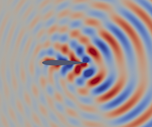
This paper focuses on linear boundary-layer receptivity in subsonic flow conditions resulting from the interaction of a surface-roughness-induced flow perturbation with a two-dimensional oblique acoustic wave emanating from the free stream; it neglects the contributions of leading-edge receptivity to the total flow instability considered in Hammerton & Kerschen (Reference Hammerton and Kerschen1996). The scattering of the acoustic wave by the wall-induced mean-flow distortion generates instabilities of viscous nature (known as first-mode or T–S waves) in zero- or favourable-pressure-gradient boundary layers, and of viscous–inviscid nature in adverse-pressure-gradient boundary layers. In the latter case, the base flow profile has an inflection point and therefore it supports Rayleigh-type unstable modes as well as T–S waves. This work is concerned with the quantification of the initial amplitude of the dominant instability (hereinafter referred to as T–S wave). A simplified diagram illustrating the acoustic-roughness receptivity problem is in figure 2. The problem formulation considers the general case of an infinite unswept wing, where streamwise instabilities tend to be the dominant transition mechanism.

Figure 2. Simplified diagram of the aerofoil acoustic-roughness receptivity problem.
2.1. Flow expansion
The total flow is modelled by the full compressible Navier–Stokes equations. Herein we assume the fluid to obey the ideal gas law and to be a calorically perfect gas. The small amplitude of the disturbances to the boundary layer allows for a double parameter expansion of the flow field to be introduced (Ruban Reference Ruban1985)
 \begin{align} \boldsymbol{q} (s,n,z,t) &= \bar{\boldsymbol{q}} (s,n) + \varepsilon_w \boldsymbol{q}_w (s,n)\,\textrm{e}^{\textrm{i} \beta z } + \varepsilon_a \boldsymbol{q}_a (s,n) \,\textrm{e}^{-\textrm{i} \omega t} \nonumber\\ &\quad +\varepsilon_w \varepsilon_a \boldsymbol{q}_b (s,n) \,\textrm{e}^{\textrm{i} \left(- \omega t + \beta z \right)} + \cdots, \end{align}
where  $\boldsymbol {q}=[u,v,w,p,\rho ,T]^{\text {T}}$ is the flow vector. The basic flow
  $\bar {\boldsymbol {q}}$ is independent of the spanwise coordinate because we idealise the wing as being infinite in the
  $z$-direction. The roughness-induced steady mean-flow distortion denoted by the subscript
  $w$ is considered to be spanwise periodic with wavenumber
  $\beta$ and to grow linearly with
  $\varepsilon _w \ll 1$, where
  $\varepsilon _w = h^{*}/c_n$ and
  $h^{*}$ is the maximum height or depth of the roughness element with respect to the baseline geometry. In turn, the acoustic perturbation denoted by the subscript
  $a$ is considered to be time harmonic with angular frequency
  $\omega$. The disturbance grows linearly with
  $\varepsilon _a=u^{*}_{a,\infty }(\varTheta _i+\alpha =0)/\bar {U}_{\infty } \ll 1$. The two-dimensional free-stream acoustic wave is incident at an angle
  $\varTheta _i \in [0,2 {\rm \pi}[$, where
  $\varTheta _i=0$ corresponds to a downstream-travelling wave (aligned with the zero-lift axis) and
  $\varTheta _i={\rm \pi} /2$ corresponds to a wave impinging on the upper surface of the aerofoil. The bi-linear flow component denoted by the subscript
  $b$ represents the unsteady perturbation correction caused by the nonlinear interaction between the flow components of order
  ${O}(\varepsilon _w)$ and
  ${O}(\varepsilon _a)$. In others words, this term represents the boundary-layer disturbance emerging from the receptivity process. The flow expansion in (2.2) captures the different components of the total flow field to first order. We neglect higher-order correction terms. The remainder of this section describes and analyses the governing equations of each of the flow components, ultimately leading to the determination of the instability wave amplitude.
2.2. Base flow
The steady basic flow problem ( $\bar {\boldsymbol {q}}(s,n$) in (2.2)) is tackled with boundary-layer theory. The pressure distribution over the body surface is obtained through an inviscid flow computation, which is then used to determine the boundary-layer solution respecting the no-slip wall condition. These two steps are described next.
2.2.1. Steady leading-order pressure distribution
There are a number of different approaches ranging in complexity and accuracy to determine the pressure field at the aerofoil surface. We solve the Euler equations directly with the open-source high-order spectral/hp element solver Nektar++ (Cantwell et al. Reference Cantwell2015). This is necessary since, in addition to extracting the pressure distribution, we require the steady inviscid solution in the entire domain as a basic flow for a linearised computation in § 2.3.2; the linear unsteady inviscid solution models the acoustic scattering field due to the incoming acoustic wave interacting with the aerofoil.
For the steady Euler solution, high-order structured meshes are generated with Gmsh (Geuzaine & Remacle Reference Geuzaine and Remacle2009). Nektar++ is parametrised to use a fourth-order discontinuous Galerkin method for the spatial discretisation. The Riemann problem at the interfaces between elements is solved with an ‘exact’ iterative method. A classical fourth-order Runge–Kutta scheme is employed for the temporal discretisation. Computations typically extend up to three convection periods of the far-field flow across the domain, guaranteeing convergence up to the desired precision.
Once a steady converged solution is attained, the pressure coefficient on the aerofoil surface,
 \begin{equation} c_p(s)=\frac{\bar{p}_e^{*}-\bar{p}_{\infty}}{\dfrac{1}{2} \bar{\rho}_{\infty} \bar{U}_\infty^{2}}, \end{equation}
is the only quantity needed to subsequently perform a steady boundary-layer computation to provide the  $\bar {\boldsymbol {q}} (s,n)$ state in (2.2), where
  $\bar {p}_e^{*}$ is the static pressure at the edge of the boundary layer to the first order of approximation. The remaining flow quantities are recovered through isentropic flow relations.
A criticism of our approach could be that the viscous–inviscid coupling is only considered up to first order, as the effects of the boundary layer on the pressure distribution are not accounted for. Higher-order boundary-layer theory could be implemented for more accurate solutions (Van Dyke Reference Van Dyke1969). However, we only consider high Reynolds number applications, for which high-order corrections of order  ${O}(R^{-1/2})$ can be neglected.
2.2.2. Steady boundary-layer field –  $\bar {\boldsymbol {q}}$

Let us denote  $\bar {\boldsymbol {q}}=[\bar {U},\bar {V},\bar {W},\bar {P}, \bar {\rho }, \bar {T}]^{\text {T}}$ the steady base flow quantities. We restrict our attention to two-dimensional flows, i.e.
  $\bar {W}=0$. It is convenient to introduce the generalised Howarth–Dorodnitsyn transformation (Moore Reference Moore1951; Stewartson Reference Stewartson1951) in order to eliminate the continuity equation from the system of equations. We define the change of variable
 \begin{equation} {\eta}=\left( \frac{\bar{U}_e^{*}}{\bar{\mu}_e^{*} \bar{\rho}_e^{*} s^{*}} \right)^{1/2} \int_0^{n^{*}} \bar{\rho}^{*}\,{\textrm{d}}s, \end{equation}
and the streamfunction
 \begin{equation} {\psi}=\left(\bar{\rho}_e^{*} \bar{\mu}_e^{*} \bar{U}_e^{*} s^{*} \right)^{1/2} {F}({\eta}, s^{*}), \end{equation}
with
 \begin{equation} F_{\eta} = \frac{{\bar{U}}^{*}}{\bar{U}_e^{*}},\quad S=\frac{{\bar{T}}^{*}}{\bar{T}_e^{*}}, \end{equation}
where the subscript ‘ $e$’ denotes boundary-layer edge quantities. For the purposes of this subsection we consider that all flow and material quantities are made non-dimensional using local boundary-layer edge quantities instead of the far-field quantities used in (2.1).
The steady boundary-layer equations (see, for example, Schlichting & Gersten Reference Schlichting and Gersten1960) are then simplified using (2.4)–(2.6a,b), yielding
 \begin{gather} \frac{\partial \left( {m_0} {F}_{{\eta} {\eta}} \right)}{\partial {\eta}} + m_3 {F}_{{\eta} {\eta}} {F} + m_1 \left( S - {F}_{{\eta}}^{2} \right) = s \left( {F}_{{\eta}} {F}_{{\eta} s} - {F}_{{\eta} {\eta}} {F}_{s} \right), \end{gather}
 \begin{gather}\frac{1}{\sigma} \frac{\partial \left({m_0} S_{{\eta}} \right)}{\partial {\eta}} + m_3 F S_{{\eta}} + {m_0} \left( \gamma-1 \right) M_e^{2} F_{{\eta} {\eta}}^{2} = s \left( F_{{\eta}} S_s - S_{{\eta}} F_s \right), \end{gather}
where,
 \begin{equation} \left.\begin{gathered} {m_0}={\bar{\mu}} {\bar{\rho}},\quad m_1=\frac{s}{\bar{U}_e^{*}} \frac{d \bar{U}_e^{*}}{d s},\quad m_2=\frac{s}{\bar{\mu}_e^{*} \bar{\rho}_e^{*}} \frac{{\textrm{d}} \left( \bar{\mu}_e^{*} \bar{\rho}_e^{*} \right)}{{\textrm{d}}s}, \\ m_3=\frac{1}{2} \left( 1+m_1+m_2 \right),\quad M_e^{2}= \frac{\bar{U}_e^{*^{2}}}{\gamma \mathcal{R} \bar{T}_e^{*}}. \end{gathered}\right\} \end{equation}
The subscripts  $\eta$ and
  $s$ indicate partial derivatives with respect to these variables. The Prandtl number, the specific heat ratio and the ideal gas constant are denoted
  $\sigma$,
  $\gamma$ and
  $\mathcal {R}$ respectively. Note that the curvature of the body has no explicit influence on the boundary layer to leading order. Curvature-related corrections appear in high-order boundary-layer theory only (Schlichting & Gersten Reference Schlichting and Gersten1960).
The usual no-slip and isothermal or adiabatic boundary conditions are used. Equation (2.7) is solved to second-order accuracy, using upwind finite differences in the streamwise direction and the fully implicit Keller-box method in the wall-normal direction. Newton iterations are used to arrive at a converged solution of the nonlinear governing equations (see more detail in § 2.5 of Raposo Reference Raposo2020). The marching procedure is stopped when the solver fails to converge due to the Goldstein singularity (Goldstein Reference Goldstein1948).
2.3. Acoustic perturbation
In this section we study the small unsteady perturbation created by a two-dimensional acoustic wave impinging on an aerofoil. We follow a technique akin to the one used for the study of the basic flow as per the illustration in figure 3. Firstly, we calculate the free-stream acoustic-wave solution analytically. We proceed to determine the inviscid acoustic flow solution in the aerofoil vicinity, which accounts for the reflection of sound off the aerofoil surface but violates the no-slip boundary condition; in this region, the steady basic flow is still inviscid but is now modified by the presence of the aerofoil. The unsteady inviscid pressure field at the aerofoil surface then drives the unsteady motion in a thin acoustic boundary layer where wall-normal pressure variations are neglected on the basis that the acoustic wavelength is large compared with the boundary-layer thickness (Goldstein Reference Goldstein1985; Ruban Reference Ruban1985). The next subsections are concerned with each of these sub-problems.

Figure 3. Schematic of the acoustic field decomposition.
2.3.1. Free-stream acoustic-wave solution
Our analysis of the acoustic field starts in the far-field region, where the uniform basic flow is unaffected by the presence of the aerofoil. Let us consider a small-amplitude acoustic wave travelling in the free stream with the unperturbed uniform steady flow,
 \begin{equation} \boldsymbol{q}_\infty(x,y,t)=\bar{\boldsymbol{q}}_\infty+ \varepsilon_a \boldsymbol{q}_{a,\infty} \varUpsilon, \end{equation}
where  $\varUpsilon = \exp \{\textrm {i} \alpha _{a} (- c_a t + x+ \lambda _1 y ) \}$ and
  $\bar {\boldsymbol {q}}_\infty =[ 1, 0, 0,\bar {p}_\infty / \bar {\rho }_\infty \bar {U}^{2}_\infty ,1,1 ]$. This implies
  $\omega =\alpha _{a} c_a$, where
  $\omega$,
  $\alpha _a$ and
  $c_a$ denote the angular frequency, streamwise wavenumber and phase speed of the wave solution. The direction of propagation of the acoustic wave is determined by parameter
  $\lambda _1$. Its relationship with the more physical angle of incidence
  $\varTheta _i$ (see definition in § 2.1) for subsonic flows is
 \begin{equation} \lambda_1=\text{tan} \left( {\rm \pi}- \varTheta_i - \alpha \right). \end{equation}
The acoustic-wave dispersion relation is known to be
 \begin{equation} c_a=1 \pm \frac{\sqrt{1+\lambda_1^{2}}}{M_\infty}, \end{equation}
whereas the acoustic-wave amplitude is
 \begin{align} u_{a,\infty}=\frac{p_{a,\infty}}{c_a-1},\quad v_{a,\infty}=\lambda_1 u_{a,\infty},\quad \theta_{a,\infty}=(\gamma-1) M_{\infty}^{2} p_{a,\infty},\quad \rho_{a,\infty}=M_{\infty}^{2} p_{a,\infty}. \end{align}
The far-field Mach number  $M_\infty =\bar {U}_\infty /\sqrt {\gamma \mathcal {R} \bar {T}_\infty }$ was introduced, as well as
  $\theta _a$ and
  $\rho _a$, the temperature and density perturbations. The acoustic pressure perturbation
  $p_{a,\infty }=1/M_\infty$ is constant with respect to the angle of incidence and corresponds to the downstream-travelling wave solution
  $u_{a,\infty }(\varTheta _i=-\alpha )=1$ (see Raposo et al. (Reference Raposo, Mughal and Ashworth2019) for more details).
2.3.2. Inviscid region
As the plane acoustic wave arriving from the far field approaches the aerofoil, the non-uniform steady basic flow modifies the acoustic wave solution. With the exception of the viscous wall layer, this flow is inviscid to leading order of approximation and is therefore adequately modelled by the linearised Euler equations for small amplitudes. Similar to the procedure adopted for the basic flow, the goal is to determine the unsteady pressure perturbation over the aerofoil surface which drives the unsteady acoustic boundary layer.
The present work uses a numerical tool developed by Bensalah (Reference Bensalah2018) to model acoustic-wave propagation in inviscid flows. Herein we will only describe the most salient points of this approach. The total flow is considered inviscid, irrotational and homentropic. Let us further consider a small-amplitude acoustic wave travelling with the potential steady basic flow,
 \begin{equation} \boldsymbol{q}(x,y,t)=\boldsymbol{q}_i(x,y)+ \varepsilon_a \boldsymbol{q}_{h}(x,y) \exp\{- \textrm{i} \omega t \}. \end{equation}
The subscript  $i$ denotes the known inviscid basic flow resulting from the computation described in § 2.2.1 and the subscript
  $h$ denotes the unknown acoustic-wave quantities, strictly a function of the coordinates
  $(x,y)$. Under these conditions the perturbation flow can be described by a potential function
  $\varphi$ according to
 \begin{equation} \boldsymbol{v}_h=\boldsymbol{\nabla} \varphi,\end{equation}
where  $\boldsymbol {v}_h=[ u_h,v_h,w_h ]^{\text {T}}$. These hypotheses, alongside a perfect gas law, allow for a simplification of the linearised Euler equations into a single scalar partial differential equation
 \begin{equation} D_t \left(c_i^{{-}2} D_t \varphi \right) - \rho_i^{{-}1} \boldsymbol{\nabla} \boldsymbol{\cdot} \left( \rho_i \boldsymbol{\nabla} \varphi \right) = 0,\end{equation}
where  $c_i=\sqrt {\gamma \mathcal {R} T_i}$ is the local speed of sound and
  $D_t=-\textrm {i}\omega + u_i \partial /\partial x+ v_i \partial /\partial y$. A detailed derivation of this equation can be found in Howe (Reference Howe1998). On solution of (2.15), we can recover the remaining physical flow variables with the scalar equations
 \begin{gather} p_h={-}\rho_i D_t \varphi, \end{gather}
 \begin{gather}\theta_h={-} \left( \gamma-1 \right) M_{\infty}^{2} D_t \varphi, \end{gather}
 \begin{gather}\rho_h={-} \rho_i c_i^{{-}2} D_t \varphi. \end{gather}
The flow respects the impermeability boundary condition at the surface of the aerofoil
 \begin{equation} \boldsymbol{\nabla} \varphi \cdot \boldsymbol{n} = 0, \end{equation}
where  $\boldsymbol {n}$ is the unit normal vector to the surface. The far-field boundary condition is not straightforward because while we know the form and amplitude of the incident acoustic wave, the reflected outgoing waves must be determined as part of the solution. The classical approach of scattering theory is to decompose the total flow as
 \begin{equation} \varphi= \varphi_r + \varphi_a, \end{equation}
where  $\varphi _r$ is the unknown reflected and scattered acoustic field, and
  $\varphi _a$ is the known far-field acoustic-wave solution determined in § 2.3.1
 \begin{equation} \varphi_a={-} \frac{\textrm{i}p_{a,\infty} }{\omega-\alpha_a } \exp \{\textrm{i}\left( \alpha_a x + k_a y \right) \}, \end{equation}
where  $k_a=\lambda _1 \alpha _a$. Substituting (2.18) into (2.15) yields
 \begin{equation} D_t \left(c_i^{{-}2} D_t \varphi_r \right) - \rho_i^{{-}1} \boldsymbol{\nabla} \boldsymbol{\cdot} \left( \rho_i \boldsymbol{\nabla} \varphi_r \right) ={-}D_t \left(c_i^{{-}2} D_t \varphi_a \right) + \rho_i^{{-}1} \boldsymbol{\nabla} \boldsymbol{\cdot} \left( \rho_i \boldsymbol{\nabla} \varphi_a \right), \end{equation}
whereas the boundary condition (2.17) becomes
 \begin{equation} \boldsymbol{\nabla} \varphi_r \cdot \boldsymbol{n} ={-} \boldsymbol{\nabla} \varphi_a \cdot \boldsymbol{n} \quad \text{at the rigid surface}. \end{equation}
In flow regions where the basic flow is uniform, the decomposition (2.18) corresponds exactly to the incident and reflected waves. In such cases, the incident acoustic wave  $\varphi _a$ satisfies the convected Helmholtz equation and therefore (2.20) is reduced to
 \begin{equation} D_t \left(c_i^{{-}2} D_t \varphi_r \right) - \rho_i^{{-}1} \boldsymbol{\nabla} \boldsymbol{\cdot} \left( \rho_i \boldsymbol{\nabla} \varphi_r \right) = 0. \end{equation}
However, as we approach the aerofoil, the term  $\varphi _r$ models not only the reflected and scattered wave solution but also the distortion of the incident acoustic wave caused by the change in the basic flow. In this case, the known right-hand side of (2.20) is non-zero and forces the appearance of an acoustic perturbation. The key advantage of introducing this decomposition is that it transforms the incident inhomogeneous boundary conditions into a forcing term of the governing equation and an inhomogeneous rigid surface boundary condition. Consequently, it becomes easier to impose boundary conditions in the far field, where a perfectly matched layer (PML) technique (Bécache, Dhia & Legendre Reference Bécache, Dhia and Legendre2004) is implemented to completely dampen the outgoing acoustic wave and avoid spurious reflections inside the computational domain. In this case, we can approximate the far-field boundary condition after the PML by
 \begin{equation} \varphi_r = 0. \end{equation}
(2.20) together with boundary conditions (2.21) and (2.23) are solved with a classic first-order finite-element code in triangular unstructured meshes generated by Gmsh (Geuzaine & Remacle Reference Geuzaine and Remacle2009). The reader is directed to Bensalah (Reference Bensalah2018) for details of the implementation. A diagram of the computational domain and a representation of the PMLs are shown in figure 4. The subscripts indicate the direction of propagation along which the sponge layer acts to dampen the solution.

Figure 4. Inviscid acoustic propagation problem – schematic diagram of the computational domain.
2.3.3. Linearised unsteady boundary-layer equations – $\boldsymbol {q}_a$

Viscous effects have thus far been neglected both in the basic flow and in the acoustic field. To correct for this, and to respect the no-slip boundary condition, we use the unsteady boundary-layer equations to model the acoustic boundary layer. Consider a perturbation superimposed on the steady boundary-layer base flow quantities,
 \begin{equation} \boldsymbol{q}(s,n,t)=\bar{\boldsymbol{q}}(s,n)+ \varepsilon_a \boldsymbol{q}_{a}(s,n) \exp\{- \textrm{i} \omega t \}. \end{equation}
The acoustic perturbations  $\boldsymbol {q}_{a}$ are functions of
  $(s,n)$, apart from the pressure perturbation considered not to vary in the wall-normal direction. Further consider the unsteady compressible boundary-layer equations
 \begin{gather} \rho_{t}+(\rho u)_{s} + (\rho v)_{n} =0, \end{gather}
 \begin{gather}\rho \left( u_{t} + u u_{s} + v u_{n} \right) ={-} p_{s} + \frac{1}{R} \left(\mu u_{n} \right)_{n}, \end{gather}
 \begin{gather}p_{n}=0, \end{gather}
 \begin{gather}\sigma \rho \left( T_{t}+ u T_{s} + v T_{n} \right) = \frac{1}{R} \left(\mu T_{n} \right)_{n} + \varGamma \left( p_{t} + u p_{s} \right) + \frac{\varGamma \mu}{R} u_n^{2}, \end{gather}
which are made non-dimensional according to (2.1), where  $R=\bar {U}_\infty c_n / \bar {\nu }_\infty$ is the global Reynolds number and
  $\varGamma =(\gamma -1) M_\infty ^{2} \sigma$. We next substitute the flow-field expansions (2.24) in the above equations, linearise around the mean flow and make a change of variable according to (2.4), yielding
 \begin{align} & \eta_n \bar{\rho} \frac{\partial v_a}{\partial \eta} + \left( \eta_s \bar{\rho}_\eta + \bar{\rho}_s \right) u_a + c_3 \left( 2 c_0 c_5 + \bar{U} (2 c_6 - c_4) -c_1 - \bar{U}_s - \textrm{i} c_2 \right) \theta_a \nonumber\\ &\quad + \eta_s \bar{\rho} \frac{\partial u_a}{\partial \eta}+ \bar{\rho} \frac{\partial u_a}{\partial s} - c_0 c_3 \frac{\partial \theta_a}{\partial \eta} + \eta_n \bar{\rho}_\eta v_a - c_3 \bar{U} \frac{\partial \theta_a}{\partial s} ={-}c_7 \bar{U} \frac{\partial p_a}{\partial s} \nonumber\\ &\quad - c_7\left( c_1 + \bar{U}_s + \textrm{i} c_2 -c_0 c_5 - c_6\bar{U} \right) p_a, \end{align}
 \begin{align} & \left[ R^{{-}1} \bar{\mu}_{\bar{T}} \bar{U}_{\eta \eta} \eta_n^{2} + R^{{-}1} \left( \bar{\mu}_{\bar{T}} \eta_{nn} + \bar{\mu}_{\bar{T} \bar{T}} \bar{T}_\eta \eta_n^{2} \right) \bar{U}_\eta + c_3 c_8 \right] \theta_a \nonumber\\ &\qquad + \frac{\bar{\mu} \eta_n^{2}}{R} \frac{\partial^{2} u_a}{\partial \eta^{2}} + R^{{-}1} \bar{\mu}_{\bar{T}} \eta_n^{2} \bar{U}_\eta \frac{\partial \theta_a}{\partial \eta}+ \left( R^{{-}1} \bar{\mu} \eta_{nn} + R^{{-}1} \bar{\mu}_{\bar{T}} \bar{T}_\eta \eta_n^{2} - \bar{\rho} c_0 \right) \frac{\partial u_a}{\partial \eta} \nonumber\\ &\qquad - \left[ \bar{\rho}\left( \eta_s \bar{U}_\eta + \bar{U}_s \right) + \textrm{i} c_2 \bar{\rho} \right] u_a - \eta_n \bar{\rho} \bar{U}_\eta v_a - \bar{\rho} \bar{U} \frac{\partial u_a}{\partial s} \nonumber\\ &\quad = \frac{\partial p_a}{\partial s} + c_7 c_8 p_a, \end{align}
 \begin{align} & 2 \eta_n^{2} R^{{-}1} \bar{\mu} \varGamma \bar{U}_\eta \frac{\partial u_a}{\partial \eta} - \left[ \sigma \bar{\rho} \left( \eta_s \bar{T}_\eta + \bar{T}_s \right) - \varGamma \bar{P}_s \right] u_a - \eta_n \sigma \bar{\rho} \bar{T}_\eta v_a + \frac{\bar{\mu} \eta_n^{2}}{R} \frac{\partial^{2} \theta_a}{\partial \eta^{2}} \nonumber\\ &\qquad - \sigma \bar{\rho} \bar{U}\frac{\partial \theta_a}{\partial s} + \left( 2 \eta_n^{2} R^{{-}1} \bar{\mu}_{\bar{T}} \bar{T}_\eta + \eta_{nn} R^{{-}1} \bar{\mu} - \sigma c_0 \bar{\rho} \right) \frac{\partial \theta_a}{\partial \eta} \nonumber\\ &\qquad + \left[ \eta_n^{2} R^{{-}1}\bar{\mu}_{\bar{T}} \bar{T}_{\eta \eta} +\eta_{nn} R^{{-}1} \bar{\mu}_{\bar{T}} \bar{T}_\eta + \eta_n^{2} R^{{-}1} \bar{\mu}_{\bar{T} \bar{T}} \bar{T}_{\eta}^{2} \right. \nonumber\\ &\qquad \left. + \sigma c_3 \left( c_0 \bar{T}_\eta + \bar{U} \bar{T}_s \right) + \eta_n^{2} R^{{-}1} \varGamma \bar{\mu}_{\bar{T}} \bar{U}_\eta^{2} - \textrm{i} c_2 \sigma \bar{\rho} \right]\theta_a \nonumber\\ &\quad = \left[ \sigma c_7 \left( c_0 \bar{T}_\eta + \bar{U} \bar{T}_s \right) - \textrm{i} c_2 \varGamma \right] p_a - \varGamma \bar{U} \frac{\partial p_a}{\partial s}, \end{align}
where
 \begin{equation} \left.\begin{gathered} c_0=\eta_s \bar{U} + \eta_n \bar{V},\quad c_1=\eta_s \bar{U}_\eta + \eta_n \bar{V}_\eta,\quad c_2={-} \omega,\quad c_3=\frac{\bar{\rho}}{\bar{T}},\quad c_4=\frac{\bar{P}_s}{\bar{P}},\\ c_5= \frac{\bar{T}_\eta}{\bar{T}},\quad c_6=\frac{\bar{T}_s}{\bar{T}}, c_7=\frac{\bar{\rho}}{\bar{P}},\quad c_8=c_0 \bar{U}_\eta + \bar{U} \bar{U}_s. \end{gathered}\right\} \end{equation}
The linearised ideal gas law closes the system of equations
 \begin{equation} \gamma M_{\infty}^{2} p_a= \bar{\rho} \theta_a + \bar{T} \rho_a. \end{equation}
The pressure perturbation  $p_a(s)$ driving the unsteady motion within the boundary layer (right-hand sides of (2.26a)–(2.26c)) is prescribed by the outer unsteady inviscid flow examined in § 2.3.2 –
  $p_h(x,y)$ evaluated at the aerofoil surface from (2.16). The corresponding flow velocity and temperature determine the boundary conditions at the edge of the boundary layer
 \begin{equation} u_a(\eta \rightarrow \infty)=\sqrt{u_h^{2}+v_h^{2}},\quad \theta_a(\eta \rightarrow \infty)=\theta_{h}, \end{equation}
where the outer layer quantities denoted by the subscript  $h$ are evaluated at the aerofoil surface (matching condition). At the wall we impose no-slip boundary conditions
 \begin{equation} u_a(s,\eta=0)=0,\quad v_a(s,\eta=0)=0,\quad \theta_a(s,\eta=0)=0. \end{equation}
The thermal fluctuation  $\theta _a$ is also assumed to have zero fluctuation at the surface. This is based on the assumption that the perturbations oscillate at high temporal frequencies. These oscillations are too fast for the thermal dynamics to react and the wall temperature to adjust (Mack Reference Mack1984).
The numerical methods to obtain a solution are very similar to those used in § 2.2.2 for the steady boundary-layer field. In this case the equations are linear and therefore Newton iterations are not required. A solution can be obtained directly once the steady boundary-layer field solution converges at each streamwise location during the parabolic numerical marching procedure (see more detail in § 2.5 of Raposo Reference Raposo2020).
2.4. Direct and adjoint linearised Navier–Stokes equations
In previous sections we have addressed the modelling of terms of  ${O}(1 )$ and
  ${O}(\varepsilon _a )$ respectively. We next discuss the treatment of the remaining terms of the double-parameter expansion (2.2).
The surface roughness causes a localised or distributed mean-flow distortion which scatters the Stokes shear wave and produces an instability wave. These two flow components are represented in (2.2) by terms of order  ${O}(\varepsilon _w)$ and
  ${O}(\varepsilon _w \varepsilon _a)$. Substitution of the flow expansion (2.2) in the full Navier–Stokes equations (A1a)–(A1e) and collection of terms of order
  ${O}(\varepsilon _w \varepsilon _a)$ yields the general form of the HLNS equations, presented symbolically as
 \begin{equation} \mathcal{L}(\omega,\beta,\bar{\boldsymbol{q}}) \boldsymbol{q}_{s,b} =\mathcal{F}(\bar{\boldsymbol{q}},\boldsymbol{q}_w,\boldsymbol{q}_a), \end{equation}
where  $\boldsymbol {q}_{s,b}=[p_b,u_b,v_b,w_b,\theta _b]^{\text {T}}$. The linearised continuity, momentum and energy equations are denoted
  $\mathcal {L}$. The bilinear forcing term
  $\mathcal {F}$ represents the interaction between the wall-induced mean-flow distortion and the Stokes layer. The explicit form of these operators for a compressible three-dimensional perturbation travelling with a three-dimensional spanwise-invariant base flow is presented in appendix B of Raposo (Reference Raposo2020). The governing equations of the mean-flow distortion are obtained by collecting terms of order
  ${O}(\varepsilon _w)$
 \begin{equation} \mathcal{L}(\omega=0,\beta,\bar{\boldsymbol{q}}) \boldsymbol{q}_{s,w} =0. \end{equation}
This is of near-identical form to the more general unsteady form given by (2.31), and can be derived by simply setting the frequency parameter  $\omega =0$ and also setting the right-hand side forcing vector
  $\mathcal {F}=0$.
Solving the systems of (2.32) and (2.31) sequentially with appropriate boundary conditions provides a direct means of quantifying the amplitude of the dominant instability wave for a prescribed surface roughness field, either localised or distributed. A schematic of the computational domain is shown in figure 5. An alternative to the direct approach, representing a more computationally efficient means to model the receptivity, is via the adjoint approach as described in Raposo et al. (Reference Raposo, Mughal and Ashworth2019). The adjoint treatment is optimally suited to study a large number of surface roughness variations. In this paper the same framework is utilised, but to account for the curved geometry of aerofoils, the HLNS and adjoint HLNS (AHLNS) are derived based on the body-fitted compressible Navier–Stokes equations. These equations are quite lengthy and not given in this paper; the interested reader is referred to appendix B of Raposo (Reference Raposo2020).

Figure 5. HLNS computational domain.
The four variants of the HLNS and AHLNS equations required to study receptivity ((2.31), (2.32) and their adjoint counterparts) all share a common numerical solver. The discretisation is based on fourth-order accurate finite differences in the streamwise direction and Chebyshev polynomials in the wall-normal direction. At the inflow, a sponge layer is used to damp upstream-travelling waves thus avoiding spurious reflections. At the outflow, radiation boundary conditions are implemented based on wavenumber estimates provided by a solution of the parabolised stability equations. The resulting large linear system of equations is solved with an efficient LU decomposition method. Further details are found in Raposo et al. (Reference Raposo, Mughal and Ashworth2019) and Raposo (Reference Raposo2020).
3. Numerical results
The acoustic receptivity model described in § 2 is applied to a NACA 0012 at  $M_\infty =0.4$. A detailed account of the stability and receptivity properties of this aerofoil is provided. This includes parametric studies on the influence of the surface roughness position and geometry, and of the acoustic-wave angle of incidence. The effects of surface curvature and of the angle of attack are also examined.
3.1. Problem definition
We consider a two-dimensional plane acoustic wave impinging on a NACA 0012 aerofoil at an angle  $\varTheta _i \in [0,2 {\rm \pi}[\ \text {rad}$. The NACA 0012 aerofoil used is based on a modified definition to give a zero-thickness trailing edge, namely
 \begin{align} y &={\pm} 0.594689181(0.298222773 \sqrt{x} - 0.127125232x - 0.357907906 x^{2} \nonumber\\ &\quad + 0.291984971 x^{3} - 0.105174606 x^{4}), \end{align}
where  $x\in [0,1]$. The maximum thickness is now approximately
  $11.894\,\%$ of the chord. We adopt a unitary chord
  $c_n=1\ \text{m}$. The aerofoil sits at an angle of attack
  $\alpha$ with respect to the incoming
  $M_\infty =0.4$ far-field uniform flow. We choose the far-field temperature
  $\bar {T}_\infty =288.2\ \text {K}$. Two different Reynolds numbers are considered throughout this section,
  $R=\{ 1, 2 \} \times 10^{6}$, but our main focus is on the first value.
Two different types of surface roughness are investigated: (i) localised Gaussian-shaped roughness positioned at  $x_b$ (or equivalently, in the body-fitted coordinate system,
  $s_b$) defined by
 \begin{equation} \hat{H}(s)=\exp \left[ - \frac{(s-s_b)^{2}}{2 \varDelta^{2}} \right], \end{equation}
where  $\varDelta$ is the non-dimensional Gaussian shape width; (ii) sinusoidally distributed roughness of wavelength
  $\lambda _w$ defined by
 \begin{equation} \hat{H}(s)=\exp \left( \textrm{i} 2 {\rm \pi}s / \lambda_w \right).\end{equation}
3.2. Basic flow
The inviscid steady Euler flow around the NACA 0012 in the absence of roughness is determined with the compressible flow solver of Nektar++ (see § 2.2.1 for details). The results were verified to converge with the domain size, mesh refinement and simulation duration. The computation takes approximately 20 h in 48 Intel(R) Xeon(R) CPU E5-2620 0 @ 2.00 GHz. A colour plot of the Mach number in the vicinity of the aerofoil is presented in figure 6(a) for  $\alpha =0^{\circ }$. In figure 6(b) we compare the pressure coefficient obtained with Nektar++ and XFOIL (Drela Reference Drela1989). Naturally, there are very small differences owing to the approximations made by XFOIL, namely the compressible flow corrections and the thin aerofoil assumption. Overall, there is very good agreement between the two approaches.

Figure 6. Inviscid steady flow field computed with the compressible Euler flow solver of Nektar++ at  $M_{\infty }=0.4$. (a) Local Mach number (
 $\alpha =0^{\circ }$). (b) Comparison of the pressure coefficient distribution at the upper surface of the aerofoil for
  $\alpha =\{-2,0,2\}^{\circ }$.
The pressure distribution is used to compute the steady boundary-layer profiles with an adiabatic boundary condition – see figure 7. CoBL is the name of the compressible boundary-layer equation solver used for the computation. Comparison with DNS (G. Chauvat & A. Hanifi 2019, private communication) shows very good agreement and thus validates the basic flow, which comprises a cornerstone in subsequent computations undertaken with the HLNS and AHLNS equations. Nonetheless, we observe a mild deterioration of the boundary-layer approximation when approaching the leading edge. This is expected since the boundary layer assumptions lose their validity at very low local Reynolds numbers. CoBL estimates laminar flow separation at  $x^{*}/c_n=0.53$. In the NACA reports of Von Doenhoff (Reference Von Doenhoff1938) and Becker (Reference Becker1940) approximate methods estimate flow separation to occur at
  $x^{*}/c_n=0.56$,
  $x^{*}/c_n=0.536$ and
  $x^{*}/c_n=0.55$. Acoustic-roughness receptivity is expected to occur upstream of this predicted flow separation point.

Figure 7. Boundary-layer profiles at  $\alpha =0^{\circ }$,
  $R=1 \times 10^{6}$. CoBL – pressure coefficient distribution obtained with Nektar++ and fed into compressible steady boundary-layer solver; DNS – G. Chauvat & A. Hanifi (private communication); (a)
  $x^{*}/c_n=0.05$, (b)
  $x^{*}/c_n=0.10$, (c)
  $x^{*}/c_n=0.15$ and (d)
  $x^{*}/c_n=0.20$.
3.3. Stability analysis
Prior to undertaking receptivity analysis, appropriate parameters to illicit a strong receptivity response need to be identified. Selecting acoustic forcing frequencies and surface roughness descriptions not attuned to the natural eigenmodes of the developing boundary layer would give rise to weak responses in the receptivity calculations. We use a standard compressible Orr–Sommerfeld solver to calculate and track the most unstable two-dimensional instabilities for a range of frequencies. This code has been used and validated extensively – the reader is referred to Mughal (Reference Mughal2006), Thomas et al. (Reference Thomas, Mughal, Gipon, Ashworth and Martinez-Cava2016), Thomas et al. (Reference Thomas, Mughal, Roland, Ashworth and Martinez-Cava2018) and Raposo (Reference Raposo2020). The resulting neutral stability curves for  $\alpha =0^{\circ }$ and two different Reynolds numbers are presented in figure 8. The edge Reynolds number
  $R_e$ and non-dimensional edge frequency
  $\omega _e$ are defined as
 \begin{equation} R_e=\frac{\bar{U}_e^{*} \bar{\rho}_e^{*} \delta_d^{*}}{\bar{\mu}_e^{*}}, \end{equation}
and
 \begin{equation} \omega_e=\frac{\omega^{*} \delta_d^{*}}{\bar{U}_e^{*}}, \end{equation}
where the subscript  $e$ denotes boundary-layer edge quantities and
  $\delta _d^{*}$ is the local displacement thickness. The neutral stability curves in figure 8(b) indicate that the most unstable eigenmode is of viscous nature close to the leading edge (
 $x^{*}<0.3\ \text {m}$). Further downstream, however, an inviscid instability mechanism plays a prominent role. This conclusion is drawn from the behaviour of the upper branch of neutral stability which seems to be slowly varying further downstream, indicating that the instability is weakly dependent on the local Reynolds number. Moreover, the upper branch of neutral stability does not tend towards zero as expected for a viscous instability and therefore is indicative of the presence of an inviscid mechanism. The pressure distribution in figure 6(b) shows that in this region there is an adverse pressure gradient; therefore the base flow has an inflection point and supports an instability of inviscid type. This is shown in figure 9 via the second derivative of the streamwise velocity profiles of the boundary layer. For locations ahead of the suction peak, the second derivative has no zero crossings and therefore there is no inflection point. Conversely, for locations after the suction peak, i.e. when the pressure gradient is adverse, an inflection point appears.

Figure 8. Neutral stability curves for  $R=1 \times 10^{6}$ (black dashed curves) and
  $R=2 \times 10^{6}$ (red solid curves) at
  $\alpha =0^{\circ }$. (a) Non-dimensional neutral stability curve. (b) Dimensional neutral stability curve for a unitary chord aerofoil with
  $\bar {T}_\infty ^{*}=288.2\ \text {K}$ and an adiabatic wall condition.

Figure 9. Second wall-normal derivative of the boundary-layer profiles at  $\alpha =0^{\circ }$,
  $R=1 \times 10^{6}$. Subscript indicates partial derivative with respect to
  $n_d=n^{*}/ \delta _d^{*}$. CoBL – pressure coefficient distribution obtained with Nektar++ and fed into compressible steady boundary-layer solver; (a)
  $x^{*}/c_n=0.05$, (b)
  $x^{*}/c_n=0.10$, (c)
  $x^{*}/c_n=0.15$ and (d)
  $x^{*}/c_n=0.20$.
The neutral curves allow us to select a number of frequencies of interest for which we track the growth of the corresponding disturbance as it convects through the boundary layer. In figure 10 we plot the  $N$-factors, a measure of the relative growth of the disturbance amplitude as the Cartesian streamwise coordinate increases. The range of frequencies were chosen to contain the ‘most dangerous’ frequency, i.e. the one that reaches
  $N=9$ at the earliest streamwise position or the one with the maximum
  $N$-factor at the end of the domain. This analysis not only yields the frequencies that we should study from the viewpoint of receptivity, but also provides an indication of the location and size of the roughness elements most effective in generating instabilities. These can be inferred from the location of the lower branch of neutral stability and from the corresponding wavelength of the disturbance.

Figure 10. The  $N$-factor curves for
  $\alpha =0^{\circ }$: (a)
  $R=1 \times 10^{6}$, frequency ranges from
  $500\ \text {Hz}$ to
  $5000\ \text {Hz}$, the interval is
  $500\ \text {Hz}$; (b)
  $R=2 \times 10^{6}$, frequency ranges from
  $2000\ \text {Hz}$ to
  $5000\ \text {Hz}$, the interval is
  $500\ \text {Hz}$.
For the remainder of this paper we focus on the conditions  $R=1 \times 10^{6}$ and
  $f^{*}=\{1000,1500,2500\} \text {Hz}$ (Strouhal number
  $\mathcal {S}=2 {\rm \pi}f^{*} c_n / \bar {U}_\infty ^{*}= \{46.16,69.24,115.4\}$). These frequencies correspond to amplification ratios of
  $N=\{2.8,4.5,6.7\}$ at the outflow of the domain
  $x^{*}/c_n=0.45$ for this particular angle of attack. The latter corresponds to the highest
  $N$-factor in this configuration and therefore is assumed particularly relevant for transition.
3.4. Acoustic field
The approach used to model the acoustic field is described in § 2.3. Having obtained the basic Euler flow around the NACA 0012, we proceed to compute the inviscid acoustic wave propagation. We choose the angle of incidence  $\varTheta _i=45^{\circ }$ and frequency
  $f^{*}=1000\ \text {Hz}$ (
 $\mathcal {S}=46.16$). This choice of frequency takes into consideration that the lower the ratio between the acoustic wavelength and the aerofoil chord, the higher the number of degrees of freedom necessary to resolve the inviscid wave–aerofoil interaction will be. In other words, higher frequencies require more computational time and memory due to having to resolve finer spatial scales in the discretisation process. All other aspects of the problem being the same, it was decided that a lower frequency would be beneficial for parametric investigations and grid convergence studies. The computational domain is defined by
  $[x_{min}, x_{max}]=[-10.0,10.0]$ and
  $[y_{min}, y_{max}]=[-5.0, 5.0]$. The useful part of the domain where the solution is considered valid is within
  $x \in [-9.5,9.0]$ and
  $y \in [-4.25, 4.25]$. Absorbing boundary conditions based on the PML formulation act to damp the solution in the remaining portion of the computational domain. The computational times are frequency-dependent because higher frequencies require finer meshes. The longest computation took approximately 3 h on a single Intel(R) Core(TM) i7-9750H CPU @ 2.60 GHz.
In figures 11(a) and 11(b) we plot the total potential function  $\varphi$ and the ‘reflected’ potential function
  $\varphi _r$, respectively. Recall from § 2.3.2 that the total flow is decomposed as
 \begin{equation} \varphi=\varphi_r+\varphi_a, \end{equation}
where  $\varphi _r$ is the unknown ‘reflected’ acoustic field and
  $\varphi _a$ is the known far-field acoustic-wave solution given by (2.19). The total potential function shows different wave–aerofoil interaction phenomena: (i) the acoustic wave is reflected at the upper surface of the aerofoil; (ii) on the underside of the aerofoil there is a shadow zone due to shielding by the aerofoil; (iii) the so-called shadow zone is narrowed by diffraction of the sound wave around the aerofoil. In addition to these phenomena, the ‘reflected’ potential function shows that an upstream-propagating wave appears as a result of reflection in the leading-edge region.

Figure 11. Real part of the complex potential functions for Strouhal number  $\mathcal {S}=46.16$ and angle of incidence
  $\varTheta _i=45^{\circ }$ at angle of attack
  $\alpha =0^{\circ }$. (a) Total potential function
  $\varphi$. (b) ‘Reflected’ potential function
  $\varphi _r$.
We extract the inviscid acoustic-wave solution on the upper surface of the aerofoil where we aim to set up and study the acoustic-roughness receptivity problem. The potential function and the streamwise velocity (in a body-fitted coordinate system) are plotted in figure 12. The remaining flow quantities are calculated with (2.14) and (2.16). Two sets of results based on a ‘coarse’ and ‘refined’ grid are presented, although they are indistinguishable. The ‘refined’ mesh has twice as many elements throughout the domain as the ‘coarse’ mesh which has 4 486 984 triangular elements. This indicates that the solution is mesh independent. Further grid refinement studies were conducted but are not shown here. A similar exercise was carried out with the PML's coefficients, which require manual tuning. We verified that the solution is independent of the value of these coefficients provided that they are large enough to adequately dampen the acoustic wave but not so large that absorption occurs too rapidly in a spatial sense.

Figure 12. Inviscid acoustic-wave solution at the upper surface of the aerofoil. Solid and dashed lines correspond to a ‘coarse’ and a ‘refined’ mesh. (a) Real (red dashed and black solid lines) and imaginary (blue dashed and black solid lines) parts of the total potential function. (b) Real (red dashed and black solid lines) and imaginary (blue dashed and black solid lines) parts of the body-fitted streamwise velocity; amplitude is represented by the dash-dotted black line.
With the inviscid acoustic problem resolved via solution of the convected Helmholtz equations (2.20), the unsteady boundary-layer acoustic signature follows immediately on solving (2.26) – see figure 13. The grid has 400 uniformly distributed points in the wall-normal direction ( $\eta \in [ 0.0,16.0]$) and 2001 points in the streamwise direction (
 $x \in [0.0,0.45]$) clustered near the leading edge according to
 \begin{equation} x_n=0.45 \left(\frac{n}{2000}\right)^{1.1} \quad n=0,2,\ldots,2000, \end{equation}
for angle of attack  $\alpha =0^{\circ }$. Further grid refinements showed the LUBLE solution to be grid independent. These studies informed the choice of exponent in (3.7).

Figure 13. Acoustic boundary-layer streamwise velocity profiles at  $x^{*}/c_n=\{0.10,0.15,0.20\}$, respectively in solid, dashed and dash-dotted lines.
3.5. Receptivity analysis
In this section we carry out receptivity analysis and parametric studies in the presence of localised and distributed surface roughness. The roughness geometries used in the analysis are given in (3.2) and (3.3). The reference length and velocity scales are the displacement thickness and the boundary-layer edge velocity at the first branch of neutral stability  $x_I$, respectively. From (2.2) it is apparent that the results are independent of the roughness height. However, note that they do depend on the choice of reference length and velocity scales. We define the receptivity amplitude
 \begin{equation} A_u(x)=\max_{y} \left( \frac{|u_b^{*}|}{\bar{U}_e^{*}} \right), \end{equation}
and the equivalent receptivity amplitude at the first branch of neutral stability  $x_I$
$x_I$
 \begin{equation} A_0=A_u (x_{I}), \end{equation}
measured through a boundary-layer stability prediction having the same amplitude in the vicinity of the second branch of neutral stability as the instability generated by surface roughness – see figure 14(a) for an example. The equivalent receptivity amplitude  $A_0$ is extracted from the solid black curve which has been matched with the direct simulation of receptivity given by the red dashed curve at
  $x=0.4$. The solid black curve is obtained by feeding an approximate eigenfunction of the boundary-layer disturbance to our HLNS solver at the inflow of the computational domain. The reason to choose this particular method to predict the boundary-layer instability growth rate is apparent in figure 14(b). Substantial non-parallel flow effects rule out use of the linear stability equations (LSE) as a suitable model. The parabolised stability equations would be a fitting alternative since its prediction of the instability amplitude evolution overlaps remarkably well with that of the HLNS result. However, the latter may prove more accurate in other conditions, for example when studying oblique waves. Moreover, using it does not come at any additional cost since this computation is needed to compute the efficiency function through the adjoint approach. The effects of surface curvature on instability growth are seen in figure 14(b) from the curves ‘HLNS – curved’ and ‘HLNS – flat’, which refer to computations including and excluding the curvature terms in the HLNS equations, respectively. These effects are practically non-existent; this is expected since T–S wave development occurs in the mid-chord region, where the radius of curvature of the aerofoil is much larger than the boundary-layer thickness.

Figure 14. Boundary-layer instability generation and growth by a localised Gaussian-shaped roughness element for Strouhal number  $\mathcal {S}=46.16$. (a) Boundary-layer instability generation by roughness element centred at
  $s_b=0.20$. Comparison between the direct HLNS solver (dashed red line) and the HLNS solver initialised with the disturbance eigenfunction (black solid line). (b) Comparison of boundary-layer instability growth predictions by different methods. All curves are indistinguishable except for LSE.
Alternatively,  $A_0$ can be calculated using the adjoint approach
 \begin{equation} A_0=|A_2| \left( \hat{H}(s) \right) A_u \left( x_I \right), \end{equation}
where  $|A_2| ( \hat {H}(s))$ is the adjoint sensitivity function (Raposo Reference Raposo2020) and
  $A_u$ now refers to the amplitude of a boundary layer disturbance used to construct the bi-orthogonality relationship; it does not concern the amplitude of the boundary-layer instability generated by the localised roughness element, which we seek to determine. Furthermore, we consider the efficiency function
 \begin{equation} | \varLambda_u | (s_b)= \frac{\sqrt{2 {\rm \pi}} |A_2| \left( \hat{H}(s) = \delta(s-s_b) \right) A_u \left( s_b \right)}{|u_a| \left(s_b,n \rightarrow \infty \right)}, \end{equation}
which is calculated for each position  $s_b$ using the local boundary-layer edge velocity and displacement thickness as the reference velocity and length scales, respectively.
The HLNS and AHLNS computations were verified to converge with the domain size and mesh size (number of Chebyshev polynomials and number of grid points in the streamwise direction). No less than 200 points per T–S wavelength are used in the streamwise direction. In the wall-normal direction we use 62 Chebyshev polynomials. The reader is referred to Raposo et al. (Reference Raposo, Mughal and Ashworth2018, Reference Raposo, Mughal and Ashworth2019) and Raposo (Reference Raposo2020) for convergence studies and extensive validation of the solver against analytical, experimental and numerical works. While the precise duration is case dependent, a typical direct computation of receptivity requires a total time of order 20 min using 20 Intel(R) Xeon(R) CPU E5-2680 0 @ 2.70 GHz. Another 20 min are required if the adjoint formulation is activated.
3.5.1. Effects of localised roughness position
In figure 15(a) we present the variation of the equivalent receptivity amplitude with the position of a Gaussian-shaped roughness element  $s_b$ for a fixed width
  $\varDelta ^{*}/c_n=7.53 \times 10^{-3}$. Two sets of results were obtained with the adjoint approach, one for each of the meshes used in the inviscid acoustic propagation calculations shown in figure 12. Acoustic receptivity is known to be very sensitive to the acoustic-wave boundary-layer signature, which in turn depends on the boundary-layer edge conditions obtained from these computations. Performing this comparison thus confirms that the inviscid acoustic propagation results are grid independent. A third set of results obtained with the direct HLNS approach is superimposed in figure 15(a). The excellent agreement with the adjoint approach supports the correctness of the implementation of both methods. In figure 15(b) we present the corresponding efficiency function using two different grids for the AHLNS computations to verify grid independence.

Figure 15. Receptivity amplitude variation with the position of the localised Gaussian-shaped roughness element for  $\mathcal {S}=46.16$,
  $\varDelta ^{*}/c_n=7.53 \times 10^{-3}$,
  $\varTheta _i=45^{\circ }$ and
  $\alpha =0^{\circ }$. First branch of neutral stability (B-I) marked by a red cross. (a) Boundary-layer instability amplitude at the first branch of neutral stability. Comparison between the direct and adjoint approach. (b) Efficiency function – HLNS grid refinement study.
We note from figure 15(a) that, unlike with zero-pressure-gradient boundary layers developing over a flat plate, receptivity is not maximal in the vicinity of the first branch of neutral stability; nor does it decay monotonically when the roughness element is located upstream or downstream of this point. Instead, non-trivial variations appear which we mostly attribute to equally non-trivial behaviour in the acoustic-wave boundary-layer signature (see figure 12b).
In figure 16 we show how the results presented in figure 15(a) change when varying the acoustic-wave angle of incidence as well as the angle of attack at a constant frequency. Firstly, note how the boundary layer is significantly more receptive to upstream-travelling waves than to downstream-travelling waves at all angles of attack. This trend is similar to what has been observed for flat plate geometries using a similar modelling approach, although in the present case the maximum does not occur for  $\varTheta _i=180^{\circ }$ (see Raposo et al. Reference Raposo, Mughal and Ashworth2019). This is largely due to the inner layer of the acoustic boundary layer, also known as the Stokes layer, having larger streamwise velocity oscillations when excited by upstream-travelling waves. The physical mechanism is most easily understood when considering the asymptotic layers of the acoustic field. Similarly to a steady boundary layer, the acoustic boundary layer is driven by an externally imposed pressure gradient. From (2.26b), it can be seen that the forcing of the streamwise momentum equation is given by
 \begin{equation} \frac{\partial p_a}{\partial s} + c_7 c_8 p_a. \end{equation}
If we neglect the plane acoustic-wave distortion by the non-uniform mean flow, it can be concluded that the streamwise pressure gradient  $\partial p_a/\partial s$ is larger for upstream-travelling waves – this is readily seen from the far-field acoustic-wave solution presented in § 2.3.1. Since acoustic receptivity is linear with respect to the acoustic field, we can thus expect upstream-travelling acoustic waves to generate T–S waves with larger initial amplitudes.

Figure 16. Equivalent receptivity amplitude variation with the position of the Gaussian-shaped roughness element. Comparison for different acoustic wave angles of incidence at three angles of attack ( $\mathcal {S}=46.16$,
  $\varDelta ^{*}/c_n=7.53 \times 10^{-3}$); (a)
  $\alpha =-2^{\circ }$, (b)
  $\alpha =0^{\circ }$ and (c)
  $\alpha =2^{\circ }$.
However, it was found in flat plate studies in Raposo (Reference Raposo2020) that viscosity plays a significant role in the acoustic reflection and hence in receptivity to highly oblique upstream-travelling waves – not accounted for in this paper, since we address the purely inviscid scattering problem presently. The LUBLE become invalid when transverse pressure variations become significant. Scale analysis of the convective terms of the  $x$-momentum equation indicates that this occurs when the streamwise wavelength of the acoustic wave is comparable to the boundary-layer thickness, i.e.
  $\delta ^{*}={O}(1/\alpha _a^{*})$. This condition is verified for high frequencies and Mach numbers, and for highly oblique upstream-travelling waves. The exact behaviour in these conditions remains an open question even in a flat plate since Raposo (Reference Raposo2020) showed that alternative theories based on the LSE fail in such conditions too.
From 16 we note how the location of the first branch of neutral stability,  $s_b=\{ 0.363,0.285,0.196\}$ for
  $\alpha =\{-2,0,2\}^{\circ }$ respectively, continues to be a reliable indicator of where receptivity is maximal for some angles of incidence, but not for others. Receptivity is typically maximal just ahead of the first branch of neutral stability because this is the location where the resonance conditions with external forcing are optimally met. This means that as the angle of attack increases, the most receptive region of the boundary layer moves upstream towards the leading edge.
Higher angles of attack are associated with stronger adverse pressure gradients in the region where the boundary layer is most receptive. For reference, the suction peak in the upper surface of the aerofoil occurs at  $x^{*}/c_n=\{0.23,0.12,0.036\}$ for
  $\alpha =\{-2,0,2\}^{\circ }$, respectively. Therefore, it can be seen from figure 16 that the boundary layer is most receptive in regions of adverse pressure gradient for the particular frequency considered. Nonetheless, there is no clear trend correlating the angle of attack and the receptivity amplitudes. Relative differences can, however, be explained qualitatively by examining the inviscid acoustic wave's slip velocity on the aerofoil upper surface shown in figure 17 for two angles of incidence of the acoustic wave. Larger amplitudes of the Stokes layer correlate with higher levels of receptivity, thus explaining the results in figure 16.

Figure 17. Inviscid acoustic-wave streamwise velocity at the upper surface of the aerofoil. Comparison for different angles of attack at two angles of incidence of the acoustic wave ( $\mathcal {S}=46.16$); (a)
  $\varTheta _i=25^{\circ }$ and (b)
  $\varTheta _i=155^{\circ }$.
Thus far we have presented and discussed results for a single frequency. In figure 18 we extend the study to higher frequencies which also correspond to higher  $N$-factors. The associated boundary-layer instabilities are thus likely to play a more prominent role in transition in this configuration. Crucially, we observe that the most receptive locations move upstream with an increase in frequency, similarly to the first branch of neutral stability. This is accompanied by an apparent decrease in receptivity amplitudes. In the next section we will see that this can be attributed to the constant width of the roughness element which does not resonate optimally for all frequencies.

Figure 18. Equivalent receptivity amplitude variation with the position of the Gaussian-shaped roughness element. Comparison for different acoustic wave angles of incidence at three frequencies ( $\alpha =0^{\circ }$,
  $\varDelta ^{*}/c_n=7.53 \times 10^{-3}$); (a)
  $\mathcal {S}=46.16$, (b)
  $\mathcal {S}=69.24$ and (c)
  $\mathcal {S}=115.4$.
3.5.2. Effects of localised roughness width
In figure 19 we show the variation of the T–S wave amplitude when changing the width of the Gaussian bump for several fixed locations  $s_b$. Parallel flow theory predicts that receptivity amplitudes vary in proportion to the Fourier transform of the surface roughness geometry, in this case
 \begin{equation} A_0 \sim \varDelta \exp\left( - 2 {\rm \pi}^{2} k^{2} \varDelta^{2} \right), \end{equation}
where  $k$ is the wavenumber. According to parallel flow theory (Choudhari Reference Choudhari1994a), the resonant wavenumber of the roughness field is given by
  $k=1/\lambda _{{TS}}-1/\lambda _{{ac}}$, where
  $\lambda _{{TS}}$ is the T–S wavelength and
  $\lambda _{{ac}}$ is the acoustic-wave streamwise wavelength. The optimal width is thus
 \begin{equation} \varDelta^{*}/c_n=\frac{\lambda_{{TS}}^{*}}{2 {\rm \pi}c_n} \frac{1}{1- \dfrac{\lambda_{{TS}}^{*}}{\lambda_{{ac}}^{*}}}, \end{equation}
where  $\lambda _{{ac}}^{*}$ can be estimated as
 \begin{equation} \lambda_{{ac}}^{*}=\left. \frac{2 {\rm \pi}|u_a^{*}|}{\dfrac{\partial |u_a^{*} |}{\partial s^{*}}} \right|_{\left( s_b, n \rightarrow \infty \right)}. \end{equation}
This result is a necessary resonant condition for receptivity stemming from (2.31) under a parallel flow assumption. For example, for  $\alpha =0^{\circ }$ and
  $s_b=\{0.15,0.25\}$, parallel flow theory predicts receptivity maxima at
  $\varDelta ^{*}/c_n=\{8.23,8.64\} \times 10^{-3}$, while our numerical approach predicts
  $\varDelta ^{*}/c_n=\{7.59,10.2\} \times 10^{-3}$. Non-parallel flow effects are thus quite substantial and should not be neglected. We note, however, that receptivity amplitudes follow similar qualitative trends to those observed in the analysis of flat plate boundary layers undertaken by Choudhari & Streett (Reference Choudhari and Streett1992). Therefore we can instead choose
  $k$ such that the maximum of (3.13) occurs for the same value of
  $\varDelta$ as observed in the numerical results. The blue dash-dotted curve in figure 19(a) superimposed on the results for
  $s_b=0.30$ shows how this model fits the numerical results. Agreement is exceptional for small roughness widths, gradually deteriorating for longer roughness elements. This is to be expected since the longer the streamwise extent of the roughness due to which receptivity arises, the more likely it is that the parallel flow assumption is invalid.

Figure 19. Equivalent receptivity amplitude variation with the width of the Gaussian-shaped roughness element. Comparison for different positions of the roughness at three angles of attack ( $\varTheta _i=45^{\circ }$,
  $\mathcal {S}=46.16$); (a)
  $\alpha =-2^{\circ }$, (b)
  $\alpha =0^{\circ }$ and (c)
  $\alpha =2^{\circ }$.
In figure 20 we show the equivalent results for three different frequencies at a fixed angle of attack  $\alpha =0^{\circ }$. Receptivity amplitudes peak at smaller widths of the roughness element for increasing frequencies – this confirms the prediction of parallel flow theory in (3.14). This also explains the apparent decrease in receptivity amplitudes for a fixed-width roughness element shown in figure 18.

Figure 20. Equivalent receptivity amplitude variation with the width of the Gaussian-shaped roughness element. Comparison for different positions of the roughness at three frequencies ( $\alpha =0^{\circ }$,
  $\varTheta _i=45^{\circ }$); (a)
  $\mathcal {S}=46.16$, (b)
  $\mathcal {S}=69.24$ and (c)
  $\mathcal {S}=115.4$.
3.5.3. Effects of sinusoidally distributed roughness wavelength
Acoustic receptivity in the presence of distributed roughness is a more interesting problem from a practical viewpoint because wing surface inhomogeneities can be characterised as a non-stationary random process, possessing irregularities over a wide range of wavelengths (Sayles & Thomas Reference Sayles and Thomas1978; Mughal & Ashworth Reference Mughal and Ashworth2013). The study of acoustic receptivity in the presence of localised roughness elements provides insight into the physical mechanisms of receptivity as well as a simpler mathematical problem. It can therefore be regarded as a cornerstone to understand the physics and study of the more general problem of continuous and discrete spectrum surface features. In fact, Choudhari & Streett (Reference Choudhari and Streett1992) proposed that receptivity to distributed roughness can be calculated as the sum of contributions from localised short-scale wall inhomogeneities. Alternatively, the study of surface features with a continuous spectrum can be decomposed into the study of sinusoidally distributed roughness via a Fourier series. This aspect motivates the results presented in this section.
The surface roughness geometry studied in this section is described in (3.3). Receptivity amplitudes as a function of the roughness wavelength are presented in figure 21 for various combinations of angle of attack and angle of incidence of the acoustic wave. The results are converged with respect to the length of the distributed roughness. This means that the roughness patch encompasses the whole region where the boundary layer is receptive and that the presence of roughness beyond this region would not alter the results.

Figure 21. Equivalent receptivity amplitude variation with the wavelength of sinusoidally distributed roughness. Comparison for different acoustic-wave angles of incidence at three angles of attack ( $\mathcal {S}=46.16$). Boundary-layer instability wavelength at the first branch of neutral stability is marked with a vertical line; (a)
  $\alpha =-2^{\circ }$, (b)
  $\alpha =0^{\circ }$ and (c)
  $\alpha =2^{\circ }$.
Receptivity amplitudes are an order of magnitude larger for distributed roughness than for localised roughness, similarly to what has been found for flat plate geometries (Choudhari & Streett Reference Choudhari and Streett1992; Raposo et al. Reference Raposo, Mughal and Ashworth2018). One striking difference, however, is that for certain angles of incidence of the acoustic wave there is a very large band of wavelengths for which the boundary layer is receptive. One such example is for  $\alpha =2^{\circ }$ and
  $\varTheta =45^{\circ }$, as opposed to the narrower bands observed for
  $\varTheta =180^{\circ }$ for example. Another difference is that maximal receptivity does not occur for wavelengths matching the boundary-layer instability wavelength. This is likely due to strong non-parallel flow effects.
Similar to the results in the previous sections, there continues to be no definitive trend when comparing receptivity at different angles of attack. Nonetheless, for most angles of incidence of the acoustic wave, amplitudes are higher at lower angles of attack. This indicates that boundary layers developing under more adverse pressure gradients are less receptive to T–S waves. This is in agreement with the findings of Crouch (Reference Crouch1994) and Raposo (Reference Raposo2020) for Falkner–Skan boundary layers. However, note that instabilities developing in adverse pressure gradients are known to be more amplified and therefore they might still be the leading cause of flow breakdown into turbulence, even though from a receptivity perspective favourable pressure gradients give rise to the largest boundary-layer disturbances.
Lastly, in figure 22 we consider the effects of varying frequency on receptivity amplitudes. It is shown that the boundary layer is undoubtedly more receptive to upstream-travelling acoustic waves than it is to its downstream-travelling counterparts. This observation is valid for all angles of attack and frequencies considered. Furthermore, an increase in frequency leads to higher receptivity amplitudes but also to markedly narrower bands of wavelengths to which the boundary layer is responsive. The fact that the boundary layer is both more receptive and more unstable for the frequency  $\mathcal {S}=115.4$ is important from a transition prediction and control perspective. It supports the assumption that this frequency plays a key role in transition in this configuration but it also suggests that implementing control strategies to minimise receptivity or reduce instability growth may be effective in delaying the onset of turbulence.

Figure 22. Equivalent receptivity amplitude variation with the wavelength of sinusoidally distributed roughness. Comparison for different acoustic-wave angles of incidence at three frequencies ( $\alpha =0^{\circ }$). Boundary-layer instability wavelength at the first branch of neutral stability is marked with a vertical line; (a)
  $\mathcal {S}=46.16$, (b)
  $\mathcal {S}=69.24$ and (c)
  $\mathcal {S}=115.4$.
4. Conclusions
The acoustic receptivity model of Raposo et al. (Reference Raposo, Mughal and Ashworth2019) based on the HLNS equations was extended to curved aerofoil geometries. This paper constitutes the first numerical study of acoustic-roughness receptivity in subsonic boundary-layer flows over aerofoils. This configuration is of much greater interest to industrial applications than flat plate geometries often considered in the literature. The distinguishing feature of this receptivity model compared with previous flat plate studies is the modelling of the acoustic field. The interaction between an incident plane acoustic wave and the aerofoil is studied by considering three distinct regions: (i) the far field where the steady flow is uniform and a solution can be obtained analytically, (ii) the region near the aerofoil where the inviscid steady flow is distorted by the presence of the aerofoil and the acoustic wave is distorted accordingly and (iii) a near-wall layer where the effects of viscosity are non-negligible both on the steady and unsteady flows. The modelling of region (ii) is made via a numerical solution of the convected Helmholtz equation. This general approach is valid for both low and high frequencies where the wavelength of the acoustic wave may be comparable to the chord of the aerofoil or many times smaller, respectively. Thus it allows for the study of receptivity of both low Mach number and near-sonic flow conditions. One limitation of this approach is that it does not account for the effects of rotational mean flow over wave–aerofoil interaction. For example the viscous boundary layer is known to have a sizeable effect on acoustic reflection for shallow angles of incidence of upstream-travelling waves (Raposo Reference Raposo2020; Raposo et al. Reference Raposo, Mughal and Ashworth2020).
In this paper, we studied a NACA 0012 aerofoil at  $R=1 \times 10^{6}$,
  $M_\infty =0.4$ and
  $\mathcal {S} \approx \{46,69,115\}$. Receptivity to viscous–inviscid instabilities on the upper surface of the aerofoil was quantified for three angles of attack in the presence of both Gaussian-shaped localised roughness and sinusoidally distributed roughness. A parametric study on the influence of the acoustic-wave angle of incidence and of surface roughness geometry was conducted. It was found that receptivity amplitudes are highest for upstream-travelling waves irrespective of the type of surface roughness, of the angle of attack or the frequency. For localised roughness, there was no clear correlation between receptivity amplitudes and the angle of attack, all other things being equal. However, the relative differences in receptivity levels appear to be qualitatively explained by the magnitude and behaviour of the inviscid acoustic-wave streamwise velocity at different angles of attack. Furthermore, it was shown that while parallel flow theory does not predict the optimal width of a Gaussian-shaped roughness element, it remains an accurate model of how receptivity amplitudes vary with the width of the roughness element. Lastly, the study of sinusoidally distributed roughness revealed a tendency for receptivity amplitudes to be higher for frequencies with higher
  $N$-factors and for lower angles of attack. In the latter case this is particularly true for upstream-travelling acoustic waves.
Acknowledgements
The authors would like to acknowledge P. Benjamin and Dr S. Rolston from Airbus CR&T for supporting a collaboration across the two teams. The authors would also like to thank the anonymous reviewers for their thoughtful comments which led to a more insightful manuscript.
Funding
This project has received funding from the European Union's Horizon 2020 research and innovation programme under the Marie Sklodowska-Curie grant agreement No 675008.
Declaration of interests
The authors report no conflict of interest.
Appendix A. Body-fitted compressible Navier–Stokes equations
The non-dimensional form of the body-fitted governing equations is (Anderson, Tannehill & Pletcher Reference Anderson, Tannehill and Pletcher2016)
 \begin{gather} \rho_t+\chi \left(\rho u \right)_s + \left(\rho v \right)_n + \left( \rho w \right)_z + \kappa \chi \rho v=0 , \end{gather}
 \begin{gather}\rho \left( u_t+\chi u u_s + v u_n + w u_z + \kappa \chi u v \right)={-}\chi p_s + \frac{\chi}{R} \left[ \frac{\partial \tau_{xx}}{\partial s} + \frac{\partial \tau_{xy} }{\partial n} + \frac{\partial \tau_{xz} }{\partial z} \right] + \frac{\kappa \chi^{2} \tau_{xy}}{R} , \end{gather}
 \begin{gather}\rho \left( v_t+\chi u v_s + v v_n + w v_z - \kappa \chi u^{2} \right)={-}p_n + \frac{\chi}{R} \left[ \frac{\partial \left( \chi \tau_{xy} \right)}{\partial s} + \frac{\partial \tau_{yy} }{\partial n} + \frac{\partial \tau_{yz} }{\partial z} \right] - \frac{ \kappa \chi \tau_{xx}}{R} , \end{gather}
 \begin{gather}{\rho} \left( w_t + \chi u w_s + v w_n + w w_z \right)={-}p_z + \frac{\chi}{R} \left[ \frac{\partial \left( \chi \tau_{xz} \right)}{\partial s} + \frac{\partial \tau_{yz} }{\partial n} + \frac{\partial \tau_{zz}}{\partial z} \right] , \\ \rho \sigma \left( T_t + \chi u T_s + v T_n + w T_z \right) = \varGamma \left(p_t + \chi u p_s + v p_n + w p_z \right) \notag\end{gather}
 \begin{gather}+ \frac{\chi}{R} \left[ \left( \chi \mu T_s \right)_s + \left( H_1 \mu T_n \right)_n + \left( H_1 \mu T_z \right)_z\right]+ \frac{\varGamma \varPhi}{R} , \end{gather}
where
 \begin{gather} \tau_{xx}=\mu \left[ \tfrac{4}{3} \chi \left( u_s + \kappa v \right) - \tfrac{2}{3} \left( v_n + w_z \right) \right], \end{gather}
 \begin{gather}\tau_{yy}= \mu \left[ \tfrac{4}{3} H_1 v_n - \tfrac{2}{3} \left( u_s +\kappa v +H_1 w_z \right) \right], \end{gather}
 \begin{gather}\tau_{zz}= \mu \left[ \tfrac{4}{3} H_1 w_z - \tfrac{2}{3} \left( u_s + \kappa v + H_1 v_n \right) \right], \end{gather}
 \begin{gather}\tau_{xz}=\mu H_1 \left( u_z+\chi w_s \right), \end{gather}
 \begin{gather}\tau_{xy}= \mu \left[ v_s + H_1^{2} \left( \chi u \right)_n \right], \end{gather}
 \begin{gather}\tau_{yz}=\mu H_1 \left( w_n + v_z \right), \end{gather}
and
 \begin{align} \frac{\varPhi}{\mu} &= 2 \left( \chi u_s + \kappa \chi v \right)^{2} + 2 v_n^{2} + 2 w_z^{2} + \left( w_n+v_z \right)^{2} + \left( u_z+\chi w_s \right)^{2} + \left( \chi v_s + H_1 \left(\chi u \right)_n \right)^{2} \nonumber\\ &\quad - \frac{2}{3} \left( \chi u_s + \kappa \chi v + v_n + w_z \right)^{2}. \end{align}
The subscripts  $t,s,n,z$ represent partial derivatives with respect to time and the curvilinear spatial coordinates. We defined the global Reynolds number
 \begin{equation} R=\frac{\bar{U}_\infty c_n}{\bar{\nu}_{\infty}}, \end{equation}
with kinematic viscosity  $\bar {\nu }_{\infty }=\bar {\mu }_{\infty }/\bar {\rho }_{\infty }$. We also defined
  $\varGamma =(\gamma -1) M_{\infty }^{2} \sigma$. The specific heat ratio is denoted
  $\gamma =1.4$, whereas
  $\sigma =0.72$ is the Prandtl number. The Mach number
  $M_{\infty }=\bar {U}_{\infty }/a_{\infty }$, with
  $a_{\infty }=\sqrt {\gamma \mathcal {R} \bar {T}_{\infty }}$, is based on far-field quantities, where
  $a_{\infty }$ is the free-stream speed of sound and
  $\mathcal {R}=287.0\ \textrm {m}^{2}\ \textrm {s}^{-2}\ \textrm {K}^{-1}$ is the ideal gas constant for air. We have also introduced the following quantities to characterise the body curvature
 \begin{equation} \kappa=\frac{1}{r_c(s)},\quad H_1=1+\kappa n, \end{equation}
where  $r_c(s)$ is the known local radius of curvature. However, a more prominent quantity in the equations of motion is
 \begin{equation} \chi=\frac{1}{H_1}. \end{equation}
The system of equations is closed with the ideal gas law
 \begin{equation} \gamma M_{\infty}^{2} {p}= {\rho} {T}, \end{equation}
and with a viscosity model. Sutherland's law is widely accepted to be the most accurate over a wide range of flow conditions
 \begin{equation} \mu=T^{{3}/{2}} \frac{1 + \dfrac{T_c}{\bar{T}_{\infty}}}{T+\dfrac{T_c}{\bar{T}_{\infty}}}, \end{equation}
where  $T_c$ is a constant value for each fluid (110.4 K for air).


