1 Introduction
Thermoacoustic interactions may generally be classified as processes involving conversions of heat to acoustic power (and vice versa). Over the past several decades, most studies of thermoacoustic phenomena are concerned with suppression of undesired acoustic waves produced spontaneously in combustion chambers due to the presence of large temperature gradients (Keller Reference Keller1995; Fleifil et al. Reference Fleifil, Annaswamy, Ghoneim and Ghoniem1996; Dowling & Morgans Reference Dowling and Morgans2005). However, the deliberate excitation of this instability by imposed temperature differences, to controllably generate self-sustained acoustic oscillations presents a growing application in the context of energy production. In this process, self-sustained oscillatory motion, accompanied by compression and expansion, generates heat transfer between the gas and a solid medium. Enhancing this effect is achieved by using a matrix of narrow channels, namely a ‘stack’, which increases the solid–gas contact area. While evidence of such devices dates back to the 19th century (Sondhauss Reference Sondhauss1850; Rijke Reference Rijke1859), a theoretical model, quantitatively capturing the phenomenon, was derived only a century later by Rott (Reference Rott1969), who formulated the linear theory of thermoacoustics, and later refined by Swift (Reference Swift1988). Swift (Reference Swift2002) extended this formulation to account for different geometric configurations, amongst which are looped-tube systems, first proposed by Ceperley (Reference Ceperley1979) and successfully demonstrated by Yazaki et al. (Reference Yazaki, Iwata, Maekawa and Tominaga1998), in which the thermodynamic cycle resembles that of Stirling heat engines. Furthermore, Ward & Swift (Reference Ward and Swift1994) developed a highly flexible numerical tool for simulation of such systems, which is widely used by designers of thermoacoustic systems.
In the majority of reported studies on thermoacoustic devices, the working fluid is one (or more) of the noble gases or air. These inert gases are widely available and are non-hazardous when pressurised, making them suitable for operation at various working conditions. In such systems, heat is transferred between the solid and gas through conduction; accordingly, these are hereinafter referred to as conduction-driven thermoacoustic systems. However, a different approach may be taken by adding a condensable gas to the working fluid such that most heat is transferred through phase change, at constant temperature, rather than conduction. In this manner, mass is exchanged between the solid and gas mixture, and the temperature gradient imposed on the stack may be reduced, allowing a system to operate at lower temperature gradients. In their work on thermoacoustic refrigeration – exploiting acoustic power to pump heat up a temperature gradient – Hiller & Swift (Reference Hiller and Swift2000) noticed condensation occurring in the cold side of the system, and concluded, using simplified models, that condensation occurred primarily on the stack walls. In a series of two papers, Raspet et al. (Reference Raspet, Slaton, Hickey and Hiller2002) and Slaton et al. (Reference Slaton, Raspet, Hickey and Hiller2002) derived the propagation equations of thermoacoustics for an air–water vapour mixture, accounting for evaporation/condensation at the stack walls, and calculated transport quantities such as acoustic power, as well as the heat and mass fluxes. Noda & Ueda (Reference Noda and Ueda2013) constructed a simple system producing acoustic oscillations using a mixture of air and water (or ethanol) as the condensable fluid. They reported a dramatic decrease in the temperature difference required for sustaining acoustic oscillations compared with a system employing dry air as the working fluid. A substantial decrease in the onset temperature difference was measured by Tsuda & Ueda (Reference Tsuda and Ueda2015, Reference Tsuda and Ueda2017) for thermoacoustic systems employing an air–water vapour gas mixture, with the latter presenting experimental results of three different system geometries corresponding to standing wave, travelling wave and a combination of the two.
Tsuda & Ueda (Reference Tsuda and Ueda2017) also measured the increase in pressure amplitude following onset of pressure oscillations in their systems. However, it appears that due to insufficient internal circulation of the finite volume of water in these closed systems, these oscillations could not maintain a limit cycle and naturally shut down shortly after the stability limit was exceeded. A similar standing-wave system with an air–water vapour gas mixture was recently reported by Meir, Offner & Ramon (Reference Meir, Offner and Ramon2018), who demonstrated the first stable operation of a thermoacoustic engine with phase change. This engine was aligned vertically such that condensed water dripped back to the stack by gravity, creating a self-contained water circulation mechanism and successfully maintaining a stable limit cycle. At the reported heat inputs, however, this mechanism could not circulate the entire volume of water initially introduced to the system. As a result, a limit cycle was maintained with a hybrid stack consisting of ‘dry’ and ‘wet’ sections, each producing acoustic power through different heat transfer mechanisms. Meir et al. (Reference Meir, Offner and Ramon2018) measured not only a dramatic decrease in the onset and limit cycle temperature differences (compared with the reference case of dry air as working gas), but also a significant increase in the produced pressure amplitude. While these studies have laid the foundations and illustrated the potential of this form of thermoacoustics, a systematic investigation of the physical mechanisms involved has yet to be performed.
In the present work, we generalise the theory of thermoacoustics with mass exchange between the solid and gas mixture, so as to account for any type of sorption process, for which phase change through evaporation/condensation is a limiting case. Configurations including any of these mechanisms are hereinafter referred to as phase-exchange thermoacoustic systems. The term ‘phase exchange’ captures all the above phenomena, noting that in sorption processes the sorbate does not change phase as in evaporation/condensation, but is absorbed (in the case of a gas–liquid system, e.g. ammonia/water) or adsorbed (in the case of a gas–solid system, e.g. water–vapour/silica) and subsequently desorbed from the sorbent material. The paper is organised as follows: § 2 is devoted to the derivation of the wave equation for linear phase-exchange thermoacoustics, subsequently used for the stability analysis as well as for calculations of the acoustic field, power and mass fluxes. In § 3 we describe the methods used for stability and limit cycle calculations, the results of which are presented and discussed in § 4, followed by concluding remarks in § 5.
2 Model formulation
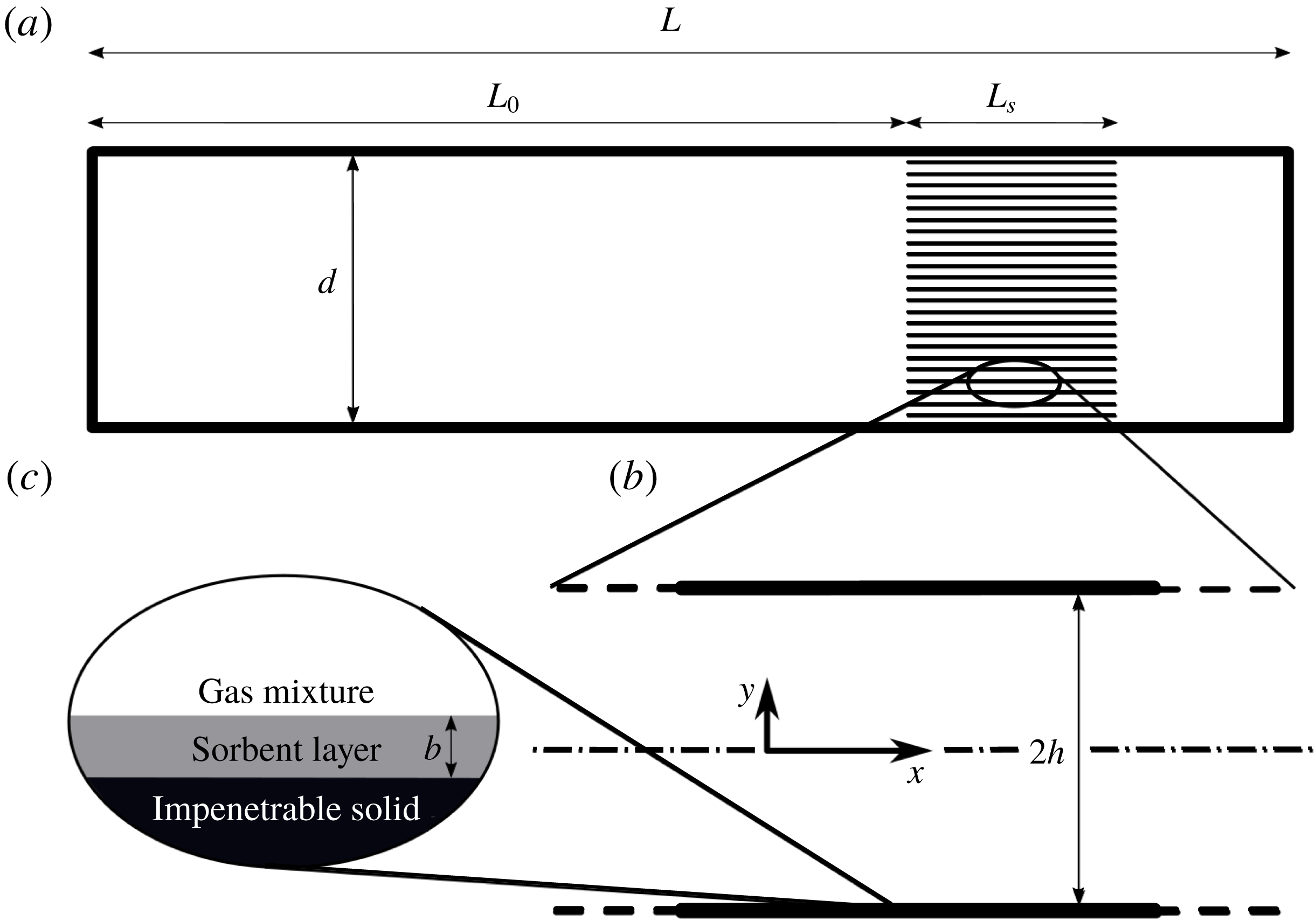
We consider a ‘stack’ of length
 $L_{s}$
placed in a straight, closed cylindrical tube of length
$L_{s}$
placed in a straight, closed cylindrical tube of length
 $L$
and diameter
$L$
and diameter
 $d$
, in which
$d$
, in which
 $d\ll L$
(see figure 1
a for a schematic illustration). The stack is comprised of multiple layers of parallel plates, spaced
$d\ll L$
(see figure 1
a for a schematic illustration). The stack is comprised of multiple layers of parallel plates, spaced
 $2h$
apart, as illustrated in figure 1(b).
$2h$
apart, as illustrated in figure 1(b).

Figure 1. System schematic drawing: (a) a grid of narrow channels (stack) of length
 $L_{s}$
located at distance
$L_{s}$
located at distance
 $L_{0}$
from a tube’s closed end, (b) representative channel of parallel plates,
$L_{0}$
from a tube’s closed end, (b) representative channel of parallel plates,
 $2h$
separated, aligned parallel to the tube axis and (c) a sorbent layer of thickness
$2h$
separated, aligned parallel to the tube axis and (c) a sorbent layer of thickness
 $b$
coating the solid impenetrable plates.
$b$
coating the solid impenetrable plates.
The working fluid in the system is a binary gas mixture comprised of a ‘reactive’ gas, able to exchange phase with the stack plates, and an inert, non-reactive gas. The governing equations describing the flow in the tube and stack channels are (Landau & Lifshitz Reference Landau and Lifshitz1959)
 $$\begin{eqnarray}\displaystyle & \displaystyle \frac{{\mathcal{D}}\unicode[STIX]{x1D70C}}{{\mathcal{D}}t}=-\unicode[STIX]{x1D70C}\unicode[STIX]{x1D735}\boldsymbol{\cdot }U, & \displaystyle\end{eqnarray}$$
 $$\begin{eqnarray}\displaystyle & \displaystyle \unicode[STIX]{x1D70C}\frac{{\mathcal{D}}U}{{\mathcal{D}}t}=-\unicode[STIX]{x1D735}p+\unicode[STIX]{x1D735}\boldsymbol{\cdot }\unicode[STIX]{x1D748}, & \displaystyle\end{eqnarray}$$
 $$\begin{eqnarray}\displaystyle & \displaystyle N\frac{{\mathcal{D}}C}{{\mathcal{D}}t}=-\unicode[STIX]{x1D735}\boldsymbol{\cdot }j, & \displaystyle\end{eqnarray}$$
 $$\begin{eqnarray}\displaystyle & \displaystyle \unicode[STIX]{x1D70C}T\frac{{\mathcal{D}}s}{{\mathcal{D}}t}=\unicode[STIX]{x1D748}\boldsymbol{ : }\unicode[STIX]{x1D735}U-\unicode[STIX]{x1D735}\boldsymbol{\cdot }(q-\unicode[STIX]{x1D707}_{c}j)-j\boldsymbol{\cdot }\unicode[STIX]{x1D735}\unicode[STIX]{x1D707}_{c}, & \displaystyle\end{eqnarray}$$
 $$\begin{eqnarray}\displaystyle & \displaystyle p=\frac{\unicode[STIX]{x1D70C}R_{g}T}{M_{mix}}, & \displaystyle\end{eqnarray}$$
namely, the mixture continuity equation, Navier–Stokes equations, mass conservation of the reactive gas, the energy equation for a gas mixture and the equation of state for an ideal gas mixture. Here
 ${\mathcal{D}}/{\mathcal{D}}t$
is the two-dimensional material derivative operator,
${\mathcal{D}}/{\mathcal{D}}t$
is the two-dimensional material derivative operator,
 $\unicode[STIX]{x1D70C}$
is the density,
$\unicode[STIX]{x1D70C}$
is the density,
 $t$
is time,
$t$
is time,
 $U\equiv \{u,v\}$
is the velocity vector comprised of the axial velocity,
$U\equiv \{u,v\}$
is the velocity vector comprised of the axial velocity,
 $u$
, and
$u$
, and
 $v$
, the transverse velocity,
$v$
, the transverse velocity,
 $p$
is the pressure,
$p$
is the pressure,
 $N$
is the molar density,
$N$
is the molar density,
 $C\equiv N_{r}/N_{mix}$
is the reactive gas concentration, expressed as a mole fraction, with subscripts ‘
$C\equiv N_{r}/N_{mix}$
is the reactive gas concentration, expressed as a mole fraction, with subscripts ‘
 $r$
’ and ‘
$r$
’ and ‘
 $mix$
’ denoting the reactive gas component and the gas mixture, respectively,
$mix$
’ denoting the reactive gas component and the gas mixture, respectively,
 $s$
is the entropy,
$s$
is the entropy,
 $\unicode[STIX]{x1D707}_{c}$
is the mixture chemical potential,
$\unicode[STIX]{x1D707}_{c}$
is the mixture chemical potential,
 $R_{g}$
is the universal gas constant,
$R_{g}$
is the universal gas constant,
 $T$
is the temperature and the mixture molar mass is defined as
$T$
is the temperature and the mixture molar mass is defined as
 $$\begin{eqnarray}M_{mix}=(M_{r}-M_{i})C+M_{i},\end{eqnarray}$$
in which
 $M_{r}$
and
$M_{r}$
and
 $M_{i}$
are the molar masses of the reactive and inert gas components, respectively. The molar and heat fluxes are (Landau & Lifshitz Reference Landau and Lifshitz1959)
$M_{i}$
are the molar masses of the reactive and inert gas components, respectively. The molar and heat fluxes are (Landau & Lifshitz Reference Landau and Lifshitz1959)
 $$\begin{eqnarray}\displaystyle & \displaystyle j=-ND\left[\unicode[STIX]{x1D735}C+\frac{k_{T}}{T}\unicode[STIX]{x1D735}T+\frac{k_{p}}{p}\unicode[STIX]{x1D735}p\right], & \displaystyle\end{eqnarray}$$
 $$\begin{eqnarray}\displaystyle & \displaystyle q=\left[k_{T}\left(\frac{\unicode[STIX]{x2202}\unicode[STIX]{x1D707}_{c}}{\unicode[STIX]{x2202}C}\right)_{p,T}-T\left(\frac{\unicode[STIX]{x2202}\unicode[STIX]{x1D707}_{c}}{\unicode[STIX]{x2202}T}\right)_{p,C}+\unicode[STIX]{x1D707}_{c}\right]j-k\unicode[STIX]{x1D735}T, & \displaystyle\end{eqnarray}$$
respectively, in which
 $D$
is the molecular diffusion coefficient,
$D$
is the molecular diffusion coefficient,
 $k$
is the thermal conductivity and
$k$
is the thermal conductivity and
 $k_{T}$
and
$k_{T}$
and
 $k_{p}$
are the thermal and baro-diffusion coefficients, respectively. The stress tensor is given by
$k_{p}$
are the thermal and baro-diffusion coefficients, respectively. The stress tensor is given by
 $$\begin{eqnarray}\unicode[STIX]{x1D748}=\unicode[STIX]{x1D707}\unicode[STIX]{x1D63F}+\unicode[STIX]{x1D709}(\unicode[STIX]{x1D735}\boldsymbol{\cdot }U)\unicode[STIX]{x1D644},\end{eqnarray}$$
where
 $\unicode[STIX]{x1D707}$
is the dynamic viscosity,
$\unicode[STIX]{x1D707}$
is the dynamic viscosity,
 $\unicode[STIX]{x1D63F}=\unicode[STIX]{x1D735}U+(\unicode[STIX]{x1D735}U)^{\text{T}}-2/3(\unicode[STIX]{x1D735}\boldsymbol{\cdot }U)\unicode[STIX]{x1D644}$
,
$\unicode[STIX]{x1D63F}=\unicode[STIX]{x1D735}U+(\unicode[STIX]{x1D735}U)^{\text{T}}-2/3(\unicode[STIX]{x1D735}\boldsymbol{\cdot }U)\unicode[STIX]{x1D644}$
,
 $\unicode[STIX]{x1D709}$
is the volume viscosity and
$\unicode[STIX]{x1D709}$
is the volume viscosity and
 $\unicode[STIX]{x1D644}$
is the identity matrix.
$\unicode[STIX]{x1D644}$
is the identity matrix.
The temperature and pressure-driven diffusion coefficients,
 $k_{T}$
and
$k_{T}$
and
 $k_{p}$
, are typically very small compared to the mass-diffusion term, as is the case considered herein, and are therefore set to zero, giving
$k_{p}$
, are typically very small compared to the mass-diffusion term, as is the case considered herein, and are therefore set to zero, giving
 $$\begin{eqnarray}\displaystyle & \displaystyle j=-ND\unicode[STIX]{x1D735}C, & \displaystyle\end{eqnarray}$$
 $$\begin{eqnarray}\displaystyle & \displaystyle q-\unicode[STIX]{x1D707}_{c}j=-\left[T\left(\frac{\unicode[STIX]{x2202}\unicode[STIX]{x1D707}_{c}}{\unicode[STIX]{x2202}T}\right)_{p,C}j+k\unicode[STIX]{x1D735}T\right]. & \displaystyle\end{eqnarray}$$
Using standard thermodynamic relations (Landau & Lifshitz Reference Landau and Lifshitz1959), we expand the entropy differential to obtain
 $$\begin{eqnarray}\text{d}s=\frac{c_{p}}{T}\,\text{d}T-\frac{\unicode[STIX]{x1D6FD}}{\unicode[STIX]{x1D70C}}\,\text{d}p-\frac{1}{M_{mix}}\left(\frac{\unicode[STIX]{x2202}\unicode[STIX]{x1D707}_{c}}{\unicode[STIX]{x2202}T}\right)_{p,C}\,\text{d}C,\end{eqnarray}$$
where
 $c_{p}$
is the heat capacity at constant pressure, and
$c_{p}$
is the heat capacity at constant pressure, and
 $\unicode[STIX]{x1D6FD}$
is the thermal expansion coefficient. Considering an ideal gas mixture we write
$\unicode[STIX]{x1D6FD}$
is the thermal expansion coefficient. Considering an ideal gas mixture we write
 $\unicode[STIX]{x1D6FD}=1/T$
and substitute (2.10)–(2.12) into (2.3) and (2.4) to obtain
$\unicode[STIX]{x1D6FD}=1/T$
and substitute (2.10)–(2.12) into (2.3) and (2.4) to obtain
 $$\begin{eqnarray}N\frac{{\mathcal{D}}C}{{\mathcal{D}}t}=\unicode[STIX]{x1D735}\boldsymbol{\cdot }(ND\unicode[STIX]{x1D735}C),\end{eqnarray}$$
 $$\begin{eqnarray}\displaystyle & & \displaystyle \unicode[STIX]{x1D70C}c_{p}\frac{{\mathcal{D}}T}{{\mathcal{D}}t}-\frac{{\mathcal{D}}p}{{\mathcal{D}}t}+\frac{p}{R_{g}}\left(\frac{\unicode[STIX]{x2202}\unicode[STIX]{x1D707}_{c}}{\unicode[STIX]{x2202}T}\right)_{p,C}\frac{{\mathcal{D}}C}{{\mathcal{D}}t}\nonumber\\ \displaystyle & & \displaystyle \quad =\unicode[STIX]{x1D70E}\boldsymbol{ : }\unicode[STIX]{x1D735}U+\unicode[STIX]{x1D735}\boldsymbol{\cdot }\left[-\frac{pD}{R_{g}}\left(\frac{\unicode[STIX]{x2202}\unicode[STIX]{x1D707}_{c}}{\unicode[STIX]{x2202}T}\right)_{p,C}\unicode[STIX]{x1D735}C+k\unicode[STIX]{x1D735}T\right]+ND\unicode[STIX]{x1D735}C\unicode[STIX]{x1D735}\unicode[STIX]{x1D707}_{c}.\end{eqnarray}$$
Equations (2.1), (2.2), (2.13) and (2.14) represent a system of nonlinear, coupled partial differential equations. In what follows, we simplify these equations through a small-parameter asymptotic approximation.
2.1 Long-wave theory approximation
The geometry of the system under consideration (as shown in figure 1) satisfies
 $h\ll d\ll L$
, allowing us to adopt a long-wave approximation in an attempt to simplify the governing equations. We begin by scaling the variables in the problem as follows
$h\ll d\ll L$
, allowing us to adopt a long-wave approximation in an attempt to simplify the governing equations. We begin by scaling the variables in the problem as follows
 $$\begin{eqnarray}\left.\begin{array}{@{}c@{}}x=\unicode[STIX]{x1D706}\hat{x};\quad y=h{\hat{y}};\quad t=\unicode[STIX]{x1D714}^{-1}\hat{t};\quad u=\unicode[STIX]{x1D714}\unicode[STIX]{x1D706}\hat{u} ;\quad v=\unicode[STIX]{x1D714}\unicode[STIX]{x1D706}\hat{v};\quad N=N_{0}\hat{N}\\ \unicode[STIX]{x1D70C}=\unicode[STIX]{x1D70C}_{0}\hat{\unicode[STIX]{x1D70C}};\quad p=\unicode[STIX]{x1D70C}_{0}\unicode[STIX]{x1D714}^{2}\unicode[STIX]{x1D706}^{2}\hat{p};\quad T={\displaystyle \frac{\unicode[STIX]{x1D714}^{2}\unicode[STIX]{x1D706}^{2}}{c_{p,0}}}\hat{T};\quad \unicode[STIX]{x1D707}_{c}={\displaystyle \frac{\unicode[STIX]{x1D714}^{2}\unicode[STIX]{x1D706}^{2}R_{g}}{c_{p,0}}}\hat{\unicode[STIX]{x1D707}_{c}},\\ \unicode[STIX]{x1D707}=\unicode[STIX]{x1D707}_{0}\hat{\unicode[STIX]{x1D707}};\quad \unicode[STIX]{x1D709}=\unicode[STIX]{x1D709}_{0}\hat{\unicode[STIX]{x1D709}};\quad D=D_{0}\hat{D};\quad c_{p}=c_{p,0}\hat{c_{p}};\quad k=k_{0}\hat{k},\end{array}\right\}\end{eqnarray}$$
where
 $\unicode[STIX]{x1D706}=a/\unicode[STIX]{x1D714}$
is the wavelength with
$\unicode[STIX]{x1D706}=a/\unicode[STIX]{x1D714}$
is the wavelength with
 $a$
denoting the speed of sound and
$a$
denoting the speed of sound and
 $\unicode[STIX]{x1D714}$
the angular frequency, subscripts ‘
$\unicode[STIX]{x1D714}$
the angular frequency, subscripts ‘
 $0$
’ denote reference values for different quantities and the hat denotes a dimensionless quantity. We define the small parameter
$0$
’ denote reference values for different quantities and the hat denotes a dimensionless quantity. We define the small parameter
 $$\begin{eqnarray}\unicode[STIX]{x1D700}=\frac{h}{\unicode[STIX]{x1D706}}\ll 1,\end{eqnarray}$$
and write the governing equations in their non-dimensional form, retaining quantities up to
 $O(\unicode[STIX]{x1D700})$
and discarding all hat signs for convenience,
$O(\unicode[STIX]{x1D700})$
and discarding all hat signs for convenience,
 $$\begin{eqnarray}\displaystyle & \displaystyle \frac{\mathfrak{D}\unicode[STIX]{x1D70C}}{\mathfrak{D}t}=-\unicode[STIX]{x1D70C}\left(\unicode[STIX]{x1D700}\frac{\unicode[STIX]{x2202}u}{\unicode[STIX]{x2202}x}+\frac{\unicode[STIX]{x2202}v}{\unicode[STIX]{x2202}y}\right), & \displaystyle\end{eqnarray}$$
 $$\begin{eqnarray}\displaystyle & \displaystyle \unicode[STIX]{x1D70C}\frac{\mathfrak{D}u}{\mathfrak{D}t}=-\unicode[STIX]{x1D700}\frac{\unicode[STIX]{x2202}p}{\unicode[STIX]{x2202}x}+\frac{\unicode[STIX]{x1D700}}{\unicode[STIX]{x1D70F}_{\unicode[STIX]{x1D708}_{0}}^{2}}\frac{\unicode[STIX]{x2202}}{\unicode[STIX]{x2202}y}\left(\unicode[STIX]{x1D707}\frac{\unicode[STIX]{x2202}u}{\unicode[STIX]{x2202}y}\right)+O(\unicode[STIX]{x1D700}^{2}), & \displaystyle\end{eqnarray}$$
 $$\begin{eqnarray}\displaystyle & \displaystyle \unicode[STIX]{x1D70C}\frac{\mathfrak{D}v}{\mathfrak{D}t}=-\frac{\unicode[STIX]{x2202}p}{\unicode[STIX]{x2202}y}+\frac{\unicode[STIX]{x1D700}}{\unicode[STIX]{x1D70F}_{\unicode[STIX]{x1D708}_{0}}^{2}}\frac{4}{3}\frac{\unicode[STIX]{x2202}}{\unicode[STIX]{x2202}y}\left(\unicode[STIX]{x1D707}\frac{\unicode[STIX]{x2202}v}{\unicode[STIX]{x2202}y}\right)+\frac{\unicode[STIX]{x1D700}}{\unicode[STIX]{x1D70F}_{\unicode[STIX]{x1D701}_{0}}^{2}}\frac{\unicode[STIX]{x2202}}{\unicode[STIX]{x2202}y}\left(\unicode[STIX]{x1D709}\frac{\unicode[STIX]{x2202}v}{\unicode[STIX]{x2202}y}\right)+O(\unicode[STIX]{x1D700}^{2}), & \displaystyle\end{eqnarray}$$
 $$\begin{eqnarray}\displaystyle & \displaystyle N\frac{\mathfrak{D}C}{\mathfrak{D}t}=\frac{\unicode[STIX]{x1D700}}{\unicode[STIX]{x1D70F}_{D_{0}}^{2}}\frac{\unicode[STIX]{x2202}}{\unicode[STIX]{x2202}y}\left(ND\frac{\unicode[STIX]{x2202}C}{\unicode[STIX]{x2202}y}\right)+O(\unicode[STIX]{x1D700}^{2}), & \displaystyle\end{eqnarray}$$
 $$\begin{eqnarray}\displaystyle & & \displaystyle \unicode[STIX]{x1D70C}c_{p}\frac{\mathfrak{D}T}{\mathfrak{D}t}-\frac{\mathfrak{D}p}{\mathfrak{D}t}-p\left(\frac{\unicode[STIX]{x2202}\unicode[STIX]{x1D707}_{c}}{\unicode[STIX]{x2202}T}\right)_{p,C}\frac{\mathfrak{D}C}{\mathfrak{D}t}\nonumber\\ \displaystyle & & \displaystyle \quad =\unicode[STIX]{x1D700}\left[\frac{\unicode[STIX]{x1D709}}{\unicode[STIX]{x1D70F}_{\unicode[STIX]{x1D701}_{0}}^{2}}\left(\frac{\unicode[STIX]{x2202}v}{\unicode[STIX]{x2202}y}\right)^{2}+\frac{\unicode[STIX]{x1D707}}{\unicode[STIX]{x1D70F}_{\unicode[STIX]{x1D708}_{0}}^{2}}\left(\left(\frac{\unicode[STIX]{x2202}u}{\unicode[STIX]{x2202}y}\right)^{2}+\frac{4}{3}\left(\frac{\unicode[STIX]{x2202}v}{\unicode[STIX]{x2202}y}\right)^{2}\right)\right]-\frac{\unicode[STIX]{x1D700}}{\unicode[STIX]{x1D70F}_{D_{0}}^{2}}\frac{p}{N}\frac{\unicode[STIX]{x2202}}{\unicode[STIX]{x2202}y}\left[\left(\frac{\unicode[STIX]{x2202}\unicode[STIX]{x1D707}_{c}}{\unicode[STIX]{x2202}T}\right)_{p,C}ND\frac{\unicode[STIX]{x2202}C}{\unicode[STIX]{x2202}y}\right]\nonumber\\ \displaystyle & & \displaystyle \qquad -\,\frac{\unicode[STIX]{x1D700}}{\unicode[STIX]{x1D70F}_{D_{0}}^{2}}\frac{p}{T}D\frac{\unicode[STIX]{x2202}C}{\unicode[STIX]{x2202}y}\left[\left(\frac{\unicode[STIX]{x2202}\unicode[STIX]{x1D707}_{c}}{\unicode[STIX]{x2202}T}\right)_{p,C}\frac{\unicode[STIX]{x2202}T}{\unicode[STIX]{x2202}y}-\frac{\unicode[STIX]{x2202}\unicode[STIX]{x1D707}_{c}}{\unicode[STIX]{x2202}y}\right]+\frac{\unicode[STIX]{x1D700}}{\unicode[STIX]{x1D70F}_{\unicode[STIX]{x1D6FC}_{0}}^{2}}\frac{\unicode[STIX]{x2202}}{\unicode[STIX]{x2202}y}\left(k\frac{\unicode[STIX]{x2202}T}{\unicode[STIX]{x2202}y}\right)+O(\unicode[STIX]{x1D700}^{2}),\end{eqnarray}$$
where
 $$\begin{eqnarray}\frac{\mathfrak{D}}{\mathfrak{D}t}\equiv \unicode[STIX]{x1D700}\left(\frac{\unicode[STIX]{x2202}}{\unicode[STIX]{x2202}t}+u\frac{\unicode[STIX]{x2202}}{\unicode[STIX]{x2202}x}\right)+v\frac{\unicode[STIX]{x2202}}{\unicode[STIX]{x2202}y}\end{eqnarray}$$
is a dimensionless material derivative operator and
 $$\begin{eqnarray}\unicode[STIX]{x1D70F}_{n_{0}}\equiv h\sqrt{\frac{\unicode[STIX]{x1D714}}{n_{0}}},\quad n=\unicode[STIX]{x1D708},\unicode[STIX]{x1D701},\unicode[STIX]{x1D6FC},D,\end{eqnarray}$$
is a dimensionless parameter representing the ratio of characteristic time scales of the acoustic oscillations and viscous, conductive and diffusive transport across the channel height, represented, respectively, by the gas properties as follows:
 $\unicode[STIX]{x1D708}_{0}\equiv \unicode[STIX]{x1D707}_{0}/\unicode[STIX]{x1D70C}_{0}$
for the kinematic viscosity,
$\unicode[STIX]{x1D708}_{0}\equiv \unicode[STIX]{x1D707}_{0}/\unicode[STIX]{x1D70C}_{0}$
for the kinematic viscosity,
 $\unicode[STIX]{x1D701}_{0}\equiv \unicode[STIX]{x1D709}_{0}/\unicode[STIX]{x1D70C}_{0}$
for the kinematic volume viscosity,
$\unicode[STIX]{x1D701}_{0}\equiv \unicode[STIX]{x1D709}_{0}/\unicode[STIX]{x1D70C}_{0}$
for the kinematic volume viscosity,
 $\unicode[STIX]{x1D6FC}_{0}\equiv k_{0}/(\unicode[STIX]{x1D70C}_{0}c_{p,0})$
for the thermal diffusivity and
$\unicode[STIX]{x1D6FC}_{0}\equiv k_{0}/(\unicode[STIX]{x1D70C}_{0}c_{p,0})$
for the thermal diffusivity and
 $D_{0}$
for the molecular diffusion coefficient.
$D_{0}$
for the molecular diffusion coefficient.
Next, we write all quantities as a series expansion of the form
 $$\begin{eqnarray}g=g_{m}(x,y)+\unicode[STIX]{x1D700}g_{1}(x,y,t)+O(\unicode[STIX]{x1D700}^{2}),\end{eqnarray}$$
in which the
 $O(1)$
term is given the subscript ‘
$O(1)$
term is given the subscript ‘
 $m$
’ (for mean) to highlight its correspondence to the quantity time-averaged value. Note that the zeroth-order, time-averaged velocities
$m$
’ (for mean) to highlight its correspondence to the quantity time-averaged value. Note that the zeroth-order, time-averaged velocities
 $u$
and
$u$
and
 $v$
are zero since the flow is purely oscillatory. We substitute these expansions into (2.17)–(2.21), and write the equations to leading order. The continuity equation for the mixture (2.17), becomes
$v$
are zero since the flow is purely oscillatory. We substitute these expansions into (2.17)–(2.21), and write the equations to leading order. The continuity equation for the mixture (2.17), becomes
 $$\begin{eqnarray}\frac{\unicode[STIX]{x2202}}{\unicode[STIX]{x2202}y}(\unicode[STIX]{x1D70C}_{m}v_{1})=0,\end{eqnarray}$$
such that
 $\unicode[STIX]{x1D70C}_{m}v_{1}=f(x,t)$
. Symmetry dictates that the transverse velocity at the mid-plane between plates,
$\unicode[STIX]{x1D70C}_{m}v_{1}=f(x,t)$
. Symmetry dictates that the transverse velocity at the mid-plane between plates,
 $v(x,0,t)$
, is zero. Since
$v(x,0,t)$
, is zero. Since
 $\unicode[STIX]{x1D70C}_{m}\neq 0$
, we have
$\unicode[STIX]{x1D70C}_{m}\neq 0$
, we have
 $v_{1}=0$
such that
$v_{1}=0$
such that
 $v=\unicode[STIX]{x1D700}^{2}v_{2}(x,y,t)+O(\unicode[STIX]{x1D700}^{3})$
. We note that since
$v=\unicode[STIX]{x1D700}^{2}v_{2}(x,y,t)+O(\unicode[STIX]{x1D700}^{3})$
. We note that since
 $v=O(\unicode[STIX]{x1D700}^{2})$
, equations (2.18) and (2.20)–(2.21) are divided by
$v=O(\unicode[STIX]{x1D700}^{2})$
, equations (2.18) and (2.20)–(2.21) are divided by
 $\unicode[STIX]{x1D700}$
to formally retain
$\unicode[STIX]{x1D700}$
to formally retain
 $O(1)$
terms. Equations (2.18)–(2.19) become, simply,
$O(1)$
terms. Equations (2.18)–(2.19) become, simply,
 $$\begin{eqnarray}\frac{\unicode[STIX]{x2202}p_{m}}{\unicode[STIX]{x2202}x}=\frac{\unicode[STIX]{x2202}p_{m}}{\unicode[STIX]{x2202}y}=0,\end{eqnarray}$$
stating that the pressure, to leading order, is constant. From (2.20) we obtain
 $$\begin{eqnarray}\frac{\unicode[STIX]{x2202}}{\unicode[STIX]{x2202}y}\left(N_{m}D_{m}\frac{\unicode[STIX]{x2202}C_{m}}{\unicode[STIX]{x2202}y}\right)=0,\end{eqnarray}$$
such that
 $N_{m}D_{m}\unicode[STIX]{x2202}C_{m}/\unicode[STIX]{x2202}y=f(x,t)$
. Symmetry requires that
$N_{m}D_{m}\unicode[STIX]{x2202}C_{m}/\unicode[STIX]{x2202}y=f(x,t)$
. Symmetry requires that
 $\unicode[STIX]{x2202}/\unicode[STIX]{x2202}y|_{y=0}=0$
is satisfied for all quantities, and since
$\unicode[STIX]{x2202}/\unicode[STIX]{x2202}y|_{y=0}=0$
is satisfied for all quantities, and since
 $N_{m},D_{m}\neq 0$
we deduce that
$N_{m},D_{m}\neq 0$
we deduce that
 $\unicode[STIX]{x2202}C_{m}/\unicode[STIX]{x2202}y=0$
. Consequently, to leading order, equation (2.21) simplifies to
$\unicode[STIX]{x2202}C_{m}/\unicode[STIX]{x2202}y=0$
. Consequently, to leading order, equation (2.21) simplifies to
 $$\begin{eqnarray}\frac{\unicode[STIX]{x2202}}{\unicode[STIX]{x2202}y}\left(k_{m}\frac{\unicode[STIX]{x2202}T_{m}}{\unicode[STIX]{x2202}y}\right)=0.\end{eqnarray}$$
Similar arguments lead to
 $\unicode[STIX]{x2202}T_{m}/\unicode[STIX]{x2202}y=0$
, noting that
$\unicode[STIX]{x2202}T_{m}/\unicode[STIX]{x2202}y=0$
, noting that
 $k_{m}\neq 0$
. The quantities
$k_{m}\neq 0$
. The quantities
 $p_{m},C_{m}$
, and
$p_{m},C_{m}$
, and
 $T_{m}$
define the zeroth-order time-averaged thermodynamic state of the gas; as these are independent of
$T_{m}$
define the zeroth-order time-averaged thermodynamic state of the gas; as these are independent of
 $y$
it follows that
$y$
it follows that
 $$\begin{eqnarray}\frac{\unicode[STIX]{x2202}g_{m}}{\unicode[STIX]{x2202}y}=0,\end{eqnarray}$$
with
 $g$
denoting any of the quantities in the system.
$g$
denoting any of the quantities in the system.
At
 $O(\unicode[STIX]{x1D700})$
, the expansion of (2.17)–(2.20) yields
$O(\unicode[STIX]{x1D700})$
, the expansion of (2.17)–(2.20) yields
 $$\begin{eqnarray}\displaystyle & \displaystyle \frac{\unicode[STIX]{x2202}\unicode[STIX]{x1D70C}_{1}}{\unicode[STIX]{x2202}t}+u_{1}\frac{\text{d}\unicode[STIX]{x1D70C}_{m}}{\text{d}x}=-\unicode[STIX]{x1D70C}_{m}\left(\frac{\unicode[STIX]{x2202}u_{1}}{\unicode[STIX]{x2202}x}+\frac{\unicode[STIX]{x2202}v_{2}}{\unicode[STIX]{x2202}y}\right), & \displaystyle\end{eqnarray}$$
 $$\begin{eqnarray}\displaystyle & \displaystyle \frac{\unicode[STIX]{x2202}u_{1}}{\unicode[STIX]{x2202}t}=-\frac{1}{\unicode[STIX]{x1D70C}_{m}}\frac{\unicode[STIX]{x2202}p_{1}}{\unicode[STIX]{x2202}x}+\frac{1}{\unicode[STIX]{x1D70F}_{\unicode[STIX]{x1D708}}^{2}}\frac{\unicode[STIX]{x2202}^{2}u_{1}}{\unicode[STIX]{x2202}y^{2}}, & \displaystyle\end{eqnarray}$$
 $$\begin{eqnarray}\displaystyle & \displaystyle \frac{\unicode[STIX]{x2202}p_{1}}{\unicode[STIX]{x2202}y}=0, & \displaystyle\end{eqnarray}$$
 $$\begin{eqnarray}\displaystyle & \displaystyle \frac{\unicode[STIX]{x2202}C_{1}}{\unicode[STIX]{x2202}t}+u_{1}\frac{\text{d}C_{m}}{\text{d}x}=\frac{1}{\unicode[STIX]{x1D70F}_{D}^{2}}\frac{\unicode[STIX]{x2202}^{2}C_{1}}{\unicode[STIX]{x2202}y^{2}}, & \displaystyle\end{eqnarray}$$
where
 $$\begin{eqnarray}\unicode[STIX]{x1D70F}_{n}=h\sqrt{\frac{\unicode[STIX]{x1D714}}{n_{m}}},\quad n=\unicode[STIX]{x1D708},D,\unicode[STIX]{x1D6FC},\end{eqnarray}$$
with
 $n$
denoting a dimensional quantity, dependent on
$n$
denoting a dimensional quantity, dependent on
 $x$
, differing from
$x$
, differing from
 $n_{0}$
which corresponds to a reference value. Using (2.32),
$n_{0}$
which corresponds to a reference value. Using (2.32),
 $O(\unicode[STIX]{x1D700})$
in (2.21) becomes
$O(\unicode[STIX]{x1D700})$
in (2.21) becomes
 $$\begin{eqnarray}\frac{\unicode[STIX]{x2202}T_{1}}{\unicode[STIX]{x2202}t}+u_{1}\frac{\text{d}T_{m}}{\text{d}x}-\frac{1}{\unicode[STIX]{x1D70C}_{m}c_{p,m}}\frac{\unicode[STIX]{x2202}p_{1}}{\unicode[STIX]{x2202}t}=\frac{1}{\unicode[STIX]{x1D70F}_{\unicode[STIX]{x1D6FC}}^{2}}\frac{\unicode[STIX]{x2202}^{2}T_{1}}{\unicode[STIX]{x2202}y^{2}}+\frac{p_{m}}{\unicode[STIX]{x1D70C}_{m}c_{p,m}}\left(\frac{\unicode[STIX]{x2202}\unicode[STIX]{x1D707}_{c}}{\unicode[STIX]{x2202}T}\right)_{p,C}\left[\frac{\unicode[STIX]{x2202}C_{1}}{\unicode[STIX]{x2202}t}+u_{1}\frac{\text{d}C_{m}}{\text{d}x}-\frac{1}{\unicode[STIX]{x1D70F}_{D}^{2}}\frac{\unicode[STIX]{x2202}^{2}C_{1}}{\unicode[STIX]{x2202}y^{2}}\right],\end{eqnarray}$$
in which the terms in square brackets sum up to zero, according to (2.33). Finally, the
 $O(\unicode[STIX]{x1D700})$
energy equation reads
$O(\unicode[STIX]{x1D700})$
energy equation reads
 $$\begin{eqnarray}\frac{\unicode[STIX]{x2202}T_{1}}{\unicode[STIX]{x2202}t}+u_{1}\frac{\text{d}T_{m}}{\text{d}x}-\frac{1}{\unicode[STIX]{x1D70C}_{m}c_{p,m}}\frac{\unicode[STIX]{x2202}p_{1}}{\unicode[STIX]{x2202}t}=\frac{1}{\unicode[STIX]{x1D70F}_{\unicode[STIX]{x1D6FC}}^{2}}\frac{\unicode[STIX]{x2202}^{2}T_{1}}{\unicode[STIX]{x2202}y^{2}}.\end{eqnarray}$$
As all governing equations, equations (2.30), (2.31), (2.33) and (2.36), contain only time-averaged terms of
 $\unicode[STIX]{x1D708}$
,
$\unicode[STIX]{x1D708}$
,
 $\unicode[STIX]{x1D6FC}$
,
$\unicode[STIX]{x1D6FC}$
,
 $D$
and
$D$
and
 $c_{p}$
, we hereinafter omit the subscript ‘
$c_{p}$
, we hereinafter omit the subscript ‘
 $m$
’ in these quantities for convenience.
$m$
’ in these quantities for convenience.
2.2 Derivation of the wave equation
The long-wave asymptotic analysis produced a set of simplified equations with all time-averaged quantities dependent only on the longitudinal coordinate
 $x$
. Next, we follow Rott (Reference Rott1969) and eliminate time dependencies by assuming harmonic oscillations. Since
$x$
. Next, we follow Rott (Reference Rott1969) and eliminate time dependencies by assuming harmonic oscillations. Since
 $t$
is scaled with
$t$
is scaled with
 $\unicode[STIX]{x1D714}^{-1}$
all variables may be expanded as
$\unicode[STIX]{x1D714}^{-1}$
all variables may be expanded as
 $g=g_{m}(x)+\unicode[STIX]{x1D700}\text{Re}[g_{1}(x,y)\text{e}^{\text{i}t}]$
, where it is recalled that
$g=g_{m}(x)+\unicode[STIX]{x1D700}\text{Re}[g_{1}(x,y)\text{e}^{\text{i}t}]$
, where it is recalled that
 $g$
denotes any of the quantities in the system. Equations (2.31), (2.33) and (2.36) then take the form
$g$
denotes any of the quantities in the system. Equations (2.31), (2.33) and (2.36) then take the form
 $$\begin{eqnarray}\displaystyle & \displaystyle \frac{\unicode[STIX]{x2202}^{2}u_{1}}{\unicode[STIX]{x2202}y^{2}}-\hat{\unicode[STIX]{x1D70F}}_{\unicode[STIX]{x1D708}}^{2}u_{1}=\frac{\unicode[STIX]{x1D70F}_{\unicode[STIX]{x1D708}}^{2}}{\unicode[STIX]{x1D70C}_{m}}\frac{\text{d}p_{1}}{\text{d}x}, & \displaystyle\end{eqnarray}$$
 $$\begin{eqnarray}\displaystyle & \displaystyle \frac{\unicode[STIX]{x2202}^{2}T_{1}}{\unicode[STIX]{x2202}y^{2}}-\hat{\unicode[STIX]{x1D70F}}_{\unicode[STIX]{x1D6FC}}^{2}T_{1}=-\frac{\hat{\unicode[STIX]{x1D70F}}_{\unicode[STIX]{x1D6FC}}^{2}}{\unicode[STIX]{x1D70C}_{m}c_{p}}p_{1}+\unicode[STIX]{x1D70F}_{\unicode[STIX]{x1D6FC}}^{2}u_{1}\frac{\text{d}T_{m}}{\text{d}x}, & \displaystyle\end{eqnarray}$$
 $$\begin{eqnarray}\displaystyle & \displaystyle \frac{\unicode[STIX]{x2202}^{2}C_{1}}{\unicode[STIX]{x2202}y^{2}}-\hat{\unicode[STIX]{x1D70F}}_{D}^{2}C_{1}=\unicode[STIX]{x1D70F}_{D}^{2}u_{1}\frac{\text{d}C_{m}}{\text{d}x}, & \displaystyle\end{eqnarray}$$
where
 $\hat{\unicode[STIX]{x1D70F}}_{n}=\text{i}^{1/2}\unicode[STIX]{x1D70F}_{n}$
. Solutions to (2.37)–(2.38) were derived by Swift (Reference Swift1988), yielding the velocity and temperature distributions
$\hat{\unicode[STIX]{x1D70F}}_{n}=\text{i}^{1/2}\unicode[STIX]{x1D70F}_{n}$
. Solutions to (2.37)–(2.38) were derived by Swift (Reference Swift1988), yielding the velocity and temperature distributions
 $$\begin{eqnarray}\displaystyle & \displaystyle u_{1}(x,y)=\frac{\text{i}H_{\unicode[STIX]{x1D708}}}{\unicode[STIX]{x1D70C}_{m}}\frac{\text{d}p_{1}}{\text{d}x}, & \displaystyle\end{eqnarray}$$
 $$\begin{eqnarray}\displaystyle & \displaystyle T_{1}(x,y)=\frac{H_{\unicode[STIX]{x1D6FC}}}{\unicode[STIX]{x1D70C}_{m}c_{p}}p_{1}+\text{i}\left[\frac{H_{\unicode[STIX]{x1D6FC}}-PrH_{\unicode[STIX]{x1D708}}}{F_{\unicode[STIX]{x1D708}}(1-Pr)}\right]\frac{\text{d}T_{m}}{\text{d}x}\langle u_{1}\rangle , & \displaystyle\end{eqnarray}$$
in which
 $Pr$
is the Prandtl number and
$Pr$
is the Prandtl number and
 $$\begin{eqnarray}\displaystyle & \displaystyle H_{n}=1-\frac{\text{cosh}(\hat{\unicode[STIX]{x1D70F}}_{n}y)}{\text{cosh}(\hat{\unicode[STIX]{x1D70F}}_{n})}, & \displaystyle\end{eqnarray}$$
 $$\begin{eqnarray}\displaystyle & \displaystyle F_{n}\equiv \int _{0}^{1}H_{n}\,\text{d}y=1-\frac{\text{tanh}(\hat{\unicode[STIX]{x1D70F}}_{n})}{\hat{\unicode[STIX]{x1D70F}}_{n}}, & \displaystyle\end{eqnarray}$$
 $$\begin{eqnarray}\displaystyle & \displaystyle \langle u_{1}\rangle \equiv \int _{0}^{1}u_{1}\,\text{d}y. & \displaystyle\end{eqnarray}$$
Solving (2.39) we note the boundary condition of symmetry at the mid-plane between plates, stating
 $\unicode[STIX]{x2202}C_{1}/\unicode[STIX]{x2202}y|_{y=0}=0$
, and the mass balance at the gas–sorbent interface (Weltsch et al.
Reference Weltsch, Offner, Liberzon and Ramon2017)
$\unicode[STIX]{x2202}C_{1}/\unicode[STIX]{x2202}y|_{y=0}=0$
, and the mass balance at the gas–sorbent interface (Weltsch et al.
Reference Weltsch, Offner, Liberzon and Ramon2017)
 $$\begin{eqnarray}\left.\frac{\unicode[STIX]{x2202}C_{1}}{\unicode[STIX]{x2202}y}\right|_{y=1}=-\frac{K\unicode[STIX]{x1D6EC}\hat{\unicode[STIX]{x1D70F}}_{D}^{2}}{1+\hat{\unicode[STIX]{x1D70F}}_{k}^{2}}\frac{N^{s}}{N_{m}}(1-C_{m})\left(\frac{C_{m}p_{1}}{p_{m}}+C_{1}|_{y=1}\right),\end{eqnarray}$$
in which the mass flux in the gas mixture, comprised of diffusion and a non-zero mixture velocity (Stefan flow), is equated to the mass flux entering/leaving the sorbent layer, expressed through a first-order sorption reaction. The sorbent layer thickness,
 $b$
(see figure 1
c), is assumed to be very small (satisfying
$b$
(see figure 1
c), is assumed to be very small (satisfying
 $\unicode[STIX]{x1D6EC}\equiv b/h\ll 1$
, with
$\unicode[STIX]{x1D6EC}\equiv b/h\ll 1$
, with
 $h$
denoting half the plate spacing) such that diffusion within the layer may be neglected and the reactive gas concentration within the sorbent cross-section is uniform.
$h$
denoting half the plate spacing) such that diffusion within the layer may be neglected and the reactive gas concentration within the sorbent cross-section is uniform.
 $K\equiv k_{a}/k_{d}$
is the equilibrium partition coefficient of the sorbent/sorbate system, with
$K\equiv k_{a}/k_{d}$
is the equilibrium partition coefficient of the sorbent/sorbate system, with
 $k_{a}$
and
$k_{a}$
and
 $k_{d}$
denoting forward and backward reaction constants, respectively,
$k_{d}$
denoting forward and backward reaction constants, respectively,
 $\hat{\unicode[STIX]{x1D70F}}_{k}\equiv (\text{i}\unicode[STIX]{x1D714}/k_{d})^{1/2}$
is a ratio of oscillation to desorption kinetics time-scales and
$\hat{\unicode[STIX]{x1D70F}}_{k}\equiv (\text{i}\unicode[STIX]{x1D714}/k_{d})^{1/2}$
is a ratio of oscillation to desorption kinetics time-scales and
 $N^{s}$
is the sorbent layer capacity for sorption of reactive gas moles per
$N^{s}$
is the sorbent layer capacity for sorption of reactive gas moles per
 $\text{m}^{3}$
. The distribution of
$\text{m}^{3}$
. The distribution of
 $C_{1}$
is then
$C_{1}$
is then
 $$\begin{eqnarray}C_{1}(x,y)=-\frac{C_{m}(1-H_{D})}{p_{m}\unicode[STIX]{x1D702}_{D}}p_{1}+\text{i}\left[\frac{1-ScH_{\unicode[STIX]{x1D708}}-{\displaystyle \frac{\unicode[STIX]{x1D702}_{\unicode[STIX]{x1D708}}}{\unicode[STIX]{x1D702}_{D}}}(1-H_{D})}{F_{\unicode[STIX]{x1D708}}(1-Sc)}\right]\frac{\text{d}C_{m}}{\text{d}x}\langle u_{1}\rangle ,\end{eqnarray}$$
in which
 $Sc$
is the Schmidt number and
$Sc$
is the Schmidt number and
 $$\begin{eqnarray}\unicode[STIX]{x1D702}_{n}=1+\frac{1+\hat{\unicode[STIX]{x1D70F}}_{k}^{2}}{K\unicode[STIX]{x1D6EC}}\frac{N_{m}}{N^{s}}\frac{1-F_{n}}{1-C_{m}},\quad n=\unicode[STIX]{x1D708},D\end{eqnarray}$$
is a parameter describing sorption kinetics. In the case of evaporation/condensation from/to a thin film, the value of
 $N^{s}$
is not constrained since the liquid has infinite capacity for condensed vapour. Accordingly,
$N^{s}$
is not constrained since the liquid has infinite capacity for condensed vapour. Accordingly,
 $N_{(Evap.)}^{s}\rightarrow \infty$
such that
$N_{(Evap.)}^{s}\rightarrow \infty$
such that
 $\unicode[STIX]{x1D702}_{n(Evap.)}\rightarrow 1$
, and
$\unicode[STIX]{x1D702}_{n(Evap.)}\rightarrow 1$
, and
 $$\begin{eqnarray}C_{1(Evap.)}(x,y)=-\frac{C_{m}}{p_{m}}(1-H_{D})p_{1}+\text{i}\left[\frac{H_{D}-ScH_{\unicode[STIX]{x1D708}}}{F_{\unicode[STIX]{x1D708}}(1-Sc)}\right]\frac{\text{d}C_{m}}{\text{d}x}\langle u_{1}\rangle .\end{eqnarray}$$
The same result is reproduced for the limit of an ‘ideal’ sorption process, in which
 $K\rightarrow \infty$
.
$K\rightarrow \infty$
.
The
 $O(\unicode[STIX]{x1D700})$
continuity equation, eliminating time derivatives, is
$O(\unicode[STIX]{x1D700})$
continuity equation, eliminating time derivatives, is
 $$\begin{eqnarray}\text{i}\unicode[STIX]{x1D70C}_{1}+u_{1}\frac{\text{d}\unicode[STIX]{x1D70C}_{m}}{\text{d}x}+\unicode[STIX]{x1D70C}_{m}\left(\frac{\unicode[STIX]{x2202}u_{1}}{\unicode[STIX]{x2202}x}+\frac{\unicode[STIX]{x2202}v_{2}}{\unicode[STIX]{x2202}y}\right)=0.\end{eqnarray}$$
The terms
 $\unicode[STIX]{x1D70C}_{1}$
and
$\unicode[STIX]{x1D70C}_{1}$
and
 $\text{d}\unicode[STIX]{x1D70C}_{m}/\text{d}x$
are derived through the total differential of the density, calculated according to (2.5)
$\text{d}\unicode[STIX]{x1D70C}_{m}/\text{d}x$
are derived through the total differential of the density, calculated according to (2.5)
 $$\begin{eqnarray}\text{d}\unicode[STIX]{x1D70C}=\frac{\unicode[STIX]{x2202}\unicode[STIX]{x1D70C}}{\unicode[STIX]{x2202}p}\text{d}p+\frac{\unicode[STIX]{x2202}\unicode[STIX]{x1D70C}}{\unicode[STIX]{x2202}T}\text{d}T+\frac{\unicode[STIX]{x2202}\unicode[STIX]{x1D70C}}{\unicode[STIX]{x2202}C}\text{d}C=\unicode[STIX]{x1D70C}\left(\frac{\text{d}p}{p}-\frac{\text{d}T}{T}+\frac{\unicode[STIX]{x1D711}\,\text{d}C}{1+\unicode[STIX]{x1D711}C}\right)\end{eqnarray}$$
in which
 $$\begin{eqnarray}\unicode[STIX]{x1D711}=\frac{M_{r}-M_{i}}{M_{i}}\end{eqnarray}$$
is a parameter containing information about the molecular masses of the two components in the mixture. The term
 $1+\unicode[STIX]{x1D711}C$
in the denominator cannot be zero since
$1+\unicode[STIX]{x1D711}C$
in the denominator cannot be zero since
 $-1<\unicode[STIX]{x1D711}$
and
$-1<\unicode[STIX]{x1D711}$
and
 $0\leqslant C\leqslant 1$
. Substituting these terms into the continuity equation, we take a cross-sectional average of (2.49), according to the definition in (2.44), to obtain
$0\leqslant C\leqslant 1$
. Substituting these terms into the continuity equation, we take a cross-sectional average of (2.49), according to the definition in (2.44), to obtain
 $$\begin{eqnarray}\text{i}\left(\frac{p_{1}}{p_{m}}-\frac{\langle T_{1}\rangle }{T_{m}}+\frac{\unicode[STIX]{x1D711}\langle C_{1}\rangle }{1+\unicode[STIX]{x1D711}C_{m}}\right)+\langle u_{1}\rangle \left(-\frac{1}{T_{m}}\frac{\text{d}T_{m}}{\text{d}x}+\frac{\unicode[STIX]{x1D711}}{1+\unicode[STIX]{x1D711}C_{m}}\frac{\text{d}C_{m}}{\text{d}x}\right)+\frac{\unicode[STIX]{x2202}\langle u_{1}\rangle }{\unicode[STIX]{x2202}x}+v_{2}|_{y=1}=0.\end{eqnarray}$$
The term
 $v_{2}|_{y=1}$
is the result of the cross-sectional average
$v_{2}|_{y=1}$
is the result of the cross-sectional average
 $$\begin{eqnarray}\left\langle \frac{\unicode[STIX]{x2202}v_{2}}{\unicode[STIX]{x2202}y}\right\rangle \equiv \int _{0}^{1}\frac{\unicode[STIX]{x2202}v_{2}}{\unicode[STIX]{x2202}y}\text{d}y=v_{2}|_{y=1}-v_{2}|_{y=0},\end{eqnarray}$$
where the transverse velocity at the mid-plane between the solid plates,
 $v_{2}|_{y=0}$
, is zero due to symmetry. The mixture velocity is given by
$v_{2}|_{y=0}$
, is zero due to symmetry. The mixture velocity is given by
 $$\begin{eqnarray}v_{2}=\frac{\unicode[STIX]{x1D70C}_{m(r)}v_{2(r)}+\unicode[STIX]{x1D70C}_{m(i)}v_{2(i)}}{\unicode[STIX]{x1D70C}_{m}},\end{eqnarray}$$
with the subscripts
 $r$
and
$r$
and
 $i$
denoting reactive and inert gas components, respectively. The relative velocity between components in a binary mixture is derived using Fick’s law (Bird, Stewart & Lightfoot Reference Bird, Stewart and Lightfoot2007), and in our scaled form is given by
$i$
denoting reactive and inert gas components, respectively. The relative velocity between components in a binary mixture is derived using Fick’s law (Bird, Stewart & Lightfoot Reference Bird, Stewart and Lightfoot2007), and in our scaled form is given by
 $$\begin{eqnarray}v_{2(r)}-v_{2(i)}=-\frac{1}{C_{m}(1-C_{m})\unicode[STIX]{x1D70F}_{D}^{2}}\frac{\unicode[STIX]{x2202}C_{1}}{\unicode[STIX]{x2202}y}.\end{eqnarray}$$
The no-penetration condition for the inert gas at the interface states
 $v_{2(i)}=0$
, such that
$v_{2(i)}=0$
, such that
 $$\begin{eqnarray}v_{2}=\frac{\unicode[STIX]{x1D70C}_{m(r)}}{\unicode[STIX]{x1D70C}_{m}}v_{2(r)}=\frac{C_{m}(1+\unicode[STIX]{x1D711})}{1+\unicode[STIX]{x1D711}C_{m}}v_{2(r)},\end{eqnarray}$$
eventually resulting in
 $$\begin{eqnarray}v_{2}|_{y=1}=-\frac{(1+\unicode[STIX]{x1D711})}{(1+\unicode[STIX]{x1D711}C_{m})(1-C_{m})\unicode[STIX]{x1D70F}_{D}^{2}}\left.\frac{\unicode[STIX]{x2202}C_{1}}{\unicode[STIX]{x2202}y}\right|_{y=1}.\end{eqnarray}$$
Substituting (2.40), (2.41), (2.46), and (2.57) into (2.52) we finally obtain the wave equation
 $$\begin{eqnarray}\frac{\text{d}}{\text{d}x}\left(\frac{F_{\unicode[STIX]{x1D708}}}{\unicode[STIX]{x1D70C}_{m}}\frac{\text{d}p_{1}}{\text{d}x}\right)+A\frac{\text{d}p_{1}}{\text{d}x}+B^{2}p_{1}=0,\end{eqnarray}$$
where
 $$\begin{eqnarray}\displaystyle & \displaystyle A=\frac{1}{\unicode[STIX]{x1D70C}_{m}}\left[\frac{F_{\unicode[STIX]{x1D6FC}}-F_{\unicode[STIX]{x1D708}}}{1-Pr}\frac{1}{T_{m}}\frac{\text{d}T_{m}}{\text{d}x}+\frac{1-F_{\unicode[STIX]{x1D708}}-{\displaystyle \frac{\unicode[STIX]{x1D702}_{\unicode[STIX]{x1D708}}}{\unicode[STIX]{x1D702}_{D}}}(1-F_{D})}{1-Sc}\frac{1}{1-C_{m}}\frac{\text{d}C_{m}}{\text{d}x}\right], & \displaystyle\end{eqnarray}$$
 $$\begin{eqnarray}\displaystyle & \displaystyle B^{2}=\frac{1}{p_{m}}\left(1-\frac{\unicode[STIX]{x1D6FE}-1}{\unicode[STIX]{x1D6FE}}F_{\unicode[STIX]{x1D6FC}}+\frac{C_{m}}{1-C_{m}}\frac{1-F_{D}}{\unicode[STIX]{x1D702}_{D}}\right). & \displaystyle\end{eqnarray}$$
In the limit
 $\unicode[STIX]{x1D702}_{n}\rightarrow 1$
, representing phase change through evaporation/condensation, equation (2.58) recovers the result of Raspet et al. (Reference Raspet, Slaton, Hickey and Hiller2002), while for
$\unicode[STIX]{x1D702}_{n}\rightarrow 1$
, representing phase change through evaporation/condensation, equation (2.58) recovers the result of Raspet et al. (Reference Raspet, Slaton, Hickey and Hiller2002), while for
 $C_{m}=\text{d}C_{m}/\text{d}x=0$
it recovers that of Rott (Reference Rott1969).
$C_{m}=\text{d}C_{m}/\text{d}x=0$
it recovers that of Rott (Reference Rott1969).
2.3 Time-averaged heat and mass fluxes
In what follows, we derive the heat and mass fluxes in an acoustic field, comprised of diffusion and acoustic ‘streaming’ – second-order, time-averaged transport quantities of the form
 $\overline{u_{1}g_{1}}=1/2\hspace{2.22198pt}\text{Re}[\langle \widetilde{u_{1}}g_{1}\rangle ]$
, where
$\overline{u_{1}g_{1}}=1/2\hspace{2.22198pt}\text{Re}[\langle \widetilde{u_{1}}g_{1}\rangle ]$
, where
 $g$
may be any scalar quantity. We first write the reactive gas mass flux and the total power flux in their dimensional form
$g$
may be any scalar quantity. We first write the reactive gas mass flux and the total power flux in their dimensional form
 $$\begin{eqnarray}\displaystyle & \displaystyle {\dot{m}}=M_{r}N_{m}\left(\frac{1}{2}\text{Re}[\langle \widetilde{u_{1}}C_{1}\rangle ]-D\frac{\text{d}C_{m}}{\text{d}x}\right), & \displaystyle\end{eqnarray}$$
 $$\begin{eqnarray}\displaystyle & \displaystyle {\dot{H}}=\unicode[STIX]{x1D70C}_{m}c_{p}\left(\frac{1}{2}\text{Re}[\langle \widetilde{u_{1}}T_{1}\rangle ]-\unicode[STIX]{x1D6FC}\frac{\text{d}T_{m}}{\text{d}x}\right)+{\dot{m}}l_{h}, & \displaystyle\end{eqnarray}$$
where
 $l_{h}$
is the reactive fluid’s heat of evaporation/sorption. The term
$l_{h}$
is the reactive fluid’s heat of evaporation/sorption. The term
 ${\dot{m}}l_{h}$
in (2.62) is the heat flux carried by the oscillating reactive gas that exchanges mass with the boundary. In scaled form, we have
${\dot{m}}l_{h}$
in (2.62) is the heat flux carried by the oscillating reactive gas that exchanges mass with the boundary. In scaled form, we have
 $$\begin{eqnarray}l_{h}=\unicode[STIX]{x1D706}^{2}\unicode[STIX]{x1D714}^{2}\widehat{l_{h}},\quad {\dot{m}}=\unicode[STIX]{x1D700}^{2}M_{r}N_{0}\unicode[STIX]{x1D706}\unicode[STIX]{x1D714}\widehat{{\dot{m}}},\quad {\dot{H}}=\unicode[STIX]{x1D700}^{2}\unicode[STIX]{x1D70C}_{0}\unicode[STIX]{x1D706}^{3}\unicode[STIX]{x1D714}^{3}\widehat{{\dot{H}}},\end{eqnarray}$$
where the mass and total power fluxes are second-order streaming effects, and are hence scaled with
 $\unicode[STIX]{x1D700}^{2}$
. The mass flux derivation appears in Weltsch et al. (Reference Weltsch, Offner, Liberzon and Ramon2017), and in our scaled form it reads
$\unicode[STIX]{x1D700}^{2}$
. The mass flux derivation appears in Weltsch et al. (Reference Weltsch, Offner, Liberzon and Ramon2017), and in our scaled form it reads
 $$\begin{eqnarray}\displaystyle {\dot{m}} & = & \displaystyle N_{m}\left\{\frac{C_{m}}{2p_{m}(1+Sc)}\text{Re}\left[\frac{\widetilde{p_{1}}u_{1}}{\unicode[STIX]{x1D702}_{D}}\left(\frac{F_{D}-\widetilde{F_{\unicode[STIX]{x1D708}}}}{\widetilde{F_{\unicode[STIX]{x1D708}}}}\right)\right]\right.\nonumber\\ \displaystyle & & \displaystyle -\left.\frac{|u_{1}|^{2}}{2(1-Sc^{2})|F_{\unicode[STIX]{x1D708}}|^{2}}\text{Im}\left[\widetilde{F_{\unicode[STIX]{x1D708}}}(1+Sc)-\frac{\unicode[STIX]{x1D702}_{\unicode[STIX]{x1D708}}}{\unicode[STIX]{x1D702}_{D}}(\widetilde{F_{\unicode[STIX]{x1D708}}}-F_{D})\right]\frac{\text{d}C_{m}}{\text{d}x}-\frac{1}{\unicode[STIX]{x1D70F}_{D}^{2}}\frac{\text{d}C_{m}}{\text{d}x}\right\},\qquad\end{eqnarray}$$
where, hereinafter, the velocity
 $u_{1}$
refers to the cross-sectionally averaged velocity, defined in (2.44), discarding the angle brackets for convenience. Using (2.64) we write the total power flux in a phase-exchange system
$u_{1}$
refers to the cross-sectionally averaged velocity, defined in (2.44), discarding the angle brackets for convenience. Using (2.64) we write the total power flux in a phase-exchange system
 $$\begin{eqnarray}\displaystyle & & \displaystyle {\dot{H}}=\frac{1}{2}\left(\frac{1}{1+Pr}\text{Re}\left[\widetilde{p_{1}}u_{1}\left(\frac{F_{\unicode[STIX]{x1D6FC}}+Pr\widetilde{F_{\unicode[STIX]{x1D708}}}}{\widetilde{F_{\unicode[STIX]{x1D708}}}}\right)\right]+\frac{C_{m}\widehat{M}N_{m}l_{h}}{p_{m}}\frac{1}{1+Sc}\text{Re}\left[\frac{\widetilde{p_{1}}u_{1}}{\unicode[STIX]{x1D702}_{D}}\left(\frac{F_{D}-\widetilde{F_{\unicode[STIX]{x1D708}}}}{\widetilde{F_{\unicode[STIX]{x1D708}}}}\right)\right]\right)\nonumber\\ \displaystyle & & \displaystyle -\,\frac{|u_{1}|^{2}}{2|F_{\unicode[STIX]{x1D708}}|^{2}}\left(\!\frac{\unicode[STIX]{x1D70C}_{m}c_{p}}{1-Pr^{2}}\text{Im}[F_{\unicode[STIX]{x1D6FC}}+Pr\widetilde{F_{\unicode[STIX]{x1D708}}}]\frac{\text{d}T_{m}}{\text{d}x}+\frac{\widehat{M}N_{m}l_{h}}{1-Sc^{2}}\text{Im}\left[\widetilde{F_{\unicode[STIX]{x1D708}}}(1+Sc)-\frac{\unicode[STIX]{x1D702}_{\unicode[STIX]{x1D708}}}{\unicode[STIX]{x1D702}_{D}}(\widetilde{F_{\unicode[STIX]{x1D708}}}-F_{D})\right]\frac{\text{d}C_{m}}{\text{d}x}\!\right)\nonumber\\ \displaystyle & & \displaystyle -\left(\frac{\unicode[STIX]{x1D70C}_{m}c_{p}}{\unicode[STIX]{x1D70F}_{\unicode[STIX]{x1D6FC}}^{2}}\frac{\text{d}T_{m}}{\text{d}x}+\frac{\widehat{M}N_{m}l_{h}}{\unicode[STIX]{x1D70F}_{D}^{2}}\frac{\text{d}C_{m}}{\text{d}x}\right),\end{eqnarray}$$
where
 $\widehat{M}\equiv M_{r}/M_{mix,0}$
is a ratio of molar masses, with
$\widehat{M}\equiv M_{r}/M_{mix,0}$
is a ratio of molar masses, with
 $M_{mix,0}$
denoting a reference value for the mixture molar mass.
$M_{mix,0}$
denoting a reference value for the mixture molar mass.
3 Solution methodology
The methods used to solve the equations describing the system stability limit and limit cycle, along with the simplifying assumptions made, are detailed and discussed below. Our analysis of a phase-exchange thermoacoustic system requires an additional definition of
 $C_{m}$
, the reactive gas time-averaged concentration (mole fraction) in the mixture. Considering equilibrium between the sorption layer and gas mixture phases (far from saturation of the sorbent),
$C_{m}$
, the reactive gas time-averaged concentration (mole fraction) in the mixture. Considering equilibrium between the sorption layer and gas mixture phases (far from saturation of the sorbent),
 $C_{m}$
must be linked with the temperature, at a given pressure. Here, the Clausius–Clapeyron relation is used, leading to
$C_{m}$
must be linked with the temperature, at a given pressure. Here, the Clausius–Clapeyron relation is used, leading to
 $$\begin{eqnarray}C_{m}=\exp \left[-\frac{l_{h}}{R}\left(\frac{1}{T_{m}}-\frac{1}{T_{max}}\right)\right],\end{eqnarray}$$
where
 $R=R_{g}/M_{r}$
is the reactive component specific gas constant,
$R=R_{g}/M_{r}$
is the reactive component specific gas constant,
 $T_{m}$
is the mean temperature and
$T_{m}$
is the mean temperature and
 $T_{max}$
is the temperature at which
$T_{max}$
is the temperature at which
 $C_{m}=1$
. The concentration gradient is then linked with the temperature gradient via
$C_{m}=1$
. The concentration gradient is then linked with the temperature gradient via
 $$\begin{eqnarray}\frac{\text{d}C_{m}}{\text{d}x}=\frac{\text{d}C_{m}}{\text{d}T_{m}}\frac{\text{d}T_{m}}{\text{d}x}=\frac{l_{h}}{R}\frac{C_{m}}{T_{m}^{2}}\frac{\text{d}T_{m}}{\text{d}x}.\end{eqnarray}$$
3.1 Stability analysis
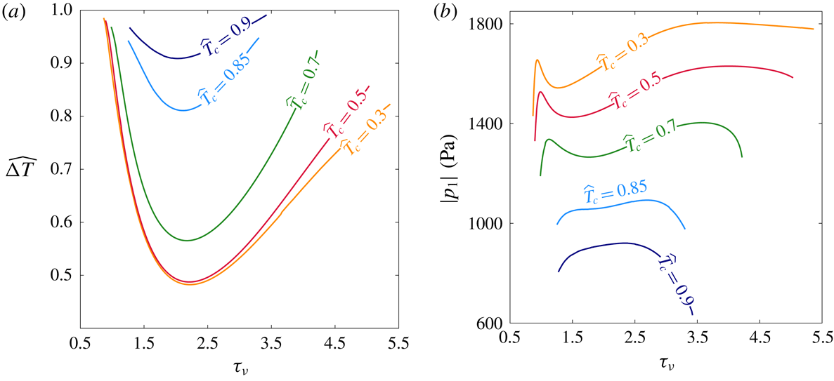
In a thermoacoustic engine converting heat into acoustic power, one side of the stack is heated (the right side in figure 1
a) while the other side is maintained at a lower temperature (the ambient, if possible). The increasing temperature gradient imposed on the stack produces acoustic power which, at first, is fully dissipated in the stack and the empty segments of the tube. The stability limit may be defined as the point at which the produced and dissipated power is exactly balanced, such that oscillations are not augmented nor decayed. At this state, a small perturbation will trigger the instability, giving rise to a growth in the amplitude of the pressure oscillations. In what follows, we seek the temperature difference
 $\unicode[STIX]{x0394}T_{onset}$
, between the two sides of the stack, sufficient for onset of the instability to occur in the system. The mean temperature profile,
$\unicode[STIX]{x0394}T_{onset}$
, between the two sides of the stack, sufficient for onset of the instability to occur in the system. The mean temperature profile,
 $T_{m}(x)$
, is generally unknown. In the empty segments of the tube it is assumed that the temperature is constant, while along the stack a temperature gradient is imposed on the solid and gas. The stack cold-side temperature,
$T_{m}(x)$
, is generally unknown. In the empty segments of the tube it is assumed that the temperature is constant, while along the stack a temperature gradient is imposed on the solid and gas. The stack cold-side temperature,
 $T_{c}$
, is assumed to be a prescribed constant. In the stable state, heat is transferred across the stack via conduction. Assuming the heating rate is sufficiently low, the temperature profile is the solution to a one-dimensional, steady-state heat equation, such that
$T_{c}$
, is assumed to be a prescribed constant. In the stable state, heat is transferred across the stack via conduction. Assuming the heating rate is sufficiently low, the temperature profile is the solution to a one-dimensional, steady-state heat equation, such that
 $\text{d}T_{m}/\text{d}x=\unicode[STIX]{x0394}T/L_{s}$
, with
$\text{d}T_{m}/\text{d}x=\unicode[STIX]{x0394}T/L_{s}$
, with
 $L_{s}$
denoting the stack length. The wave equation, equation (2.58), is then a linear, homogeneous ordinary differential equation. The stability limit is sought by targeting the non-trivial solution satisfying the eigenvalue problem. We present two different methods for solving this problem: the first is a numerical scheme, while the second is a semi-analytic, simple approach involving acoustic power calculations.
$L_{s}$
denoting the stack length. The wave equation, equation (2.58), is then a linear, homogeneous ordinary differential equation. The stability limit is sought by targeting the non-trivial solution satisfying the eigenvalue problem. We present two different methods for solving this problem: the first is a numerical scheme, while the second is a semi-analytic, simple approach involving acoustic power calculations.
3.1.1 Finite differences scheme
In this numerical scheme we approximate pressure and velocity derivatives using finite differences, obtaining a linear, homogeneous set of equations. We begin by writing (2.58) as two first-order ordinary differential equations (ODEs) for the pressure and velocity oscillations
 $$\begin{eqnarray}\displaystyle & \displaystyle \frac{\text{d}p_{1}}{\text{d}x}=-\frac{\text{i}\unicode[STIX]{x1D70C}_{m}}{F_{\unicode[STIX]{x1D708}}}u_{1}, & \displaystyle\end{eqnarray}$$
 $$\begin{eqnarray}\displaystyle & \displaystyle \frac{\text{d}u_{1}}{\text{d}x}=-\text{i}B^{2}p_{1}-\frac{A}{F_{\unicode[STIX]{x1D708}}}u_{1}, & \displaystyle\end{eqnarray}$$
where
 $A$
and
$A$
and
 $B$
are defined in (2.59)–(2.60). In order to solve the system of equations, the tube is divided into
$B$
are defined in (2.59)–(2.60). In order to solve the system of equations, the tube is divided into
 $n$
equally spaced intervals, each interval
$n$
equally spaced intervals, each interval
 $\unicode[STIX]{x0394}x=L/n$
long. The derivatives
$\unicode[STIX]{x0394}x=L/n$
long. The derivatives
 $\text{d}p_{1}/\text{d}x$
and
$\text{d}p_{1}/\text{d}x$
and
 $\text{d}u_{1}/\text{d}x$
are expressed using forward differences, such that (3.3) and (3.4) are translated into
$\text{d}u_{1}/\text{d}x$
are expressed using forward differences, such that (3.3) and (3.4) are translated into
 $2n$
equations. The remaining 2 equations arise from boundary conditions, demanding
$2n$
equations. The remaining 2 equations arise from boundary conditions, demanding
 $u_{1,1}=u_{1,n+1}=0$
, namely that the velocity is zero at the closed ends. Ultimately, the following system is obtained
$u_{1,1}=u_{1,n+1}=0$
, namely that the velocity is zero at the closed ends. Ultimately, the following system is obtained
 $$\begin{eqnarray}\unicode[STIX]{x1D63C}\left(\begin{array}{@{}c@{}}p_{1,1}\\ \vdots \\ p_{1,n+1}\\ u_{1,1}\\ \vdots \\ u_{1,n+1}\end{array}\right)=0,\end{eqnarray}$$
where
 $\unicode[STIX]{x1D63C}$
is the coefficients matrix, and the vector comprises pressure and velocity at all the discrete points in the system. We seek the non-trivial solution by setting
$\unicode[STIX]{x1D63C}$
is the coefficients matrix, and the vector comprises pressure and velocity at all the discrete points in the system. We seek the non-trivial solution by setting
 $\text{det}(\unicode[STIX]{x1D63C})=0$
. Since
$\text{det}(\unicode[STIX]{x1D63C})=0$
. Since
 $\unicode[STIX]{x1D63C}\in \mathbb{C}$
, guesses for two variables in
$\unicode[STIX]{x1D63C}\in \mathbb{C}$
, guesses for two variables in
 $\unicode[STIX]{x1D63C}$
are required to allow the use of a gradient-based method, targeting
$\unicode[STIX]{x1D63C}$
are required to allow the use of a gradient-based method, targeting
 $\text{Re}[\text{det}(\unicode[STIX]{x1D63C})]=\text{Im}[\text{det}(\unicode[STIX]{x1D63C})]=0$
. Our guesses are the resonant frequency,
$\text{Re}[\text{det}(\unicode[STIX]{x1D63C})]=\text{Im}[\text{det}(\unicode[STIX]{x1D63C})]=0$
. Our guesses are the resonant frequency,
 $\unicode[STIX]{x1D714}$
, and the temperature difference on the stack,
$\unicode[STIX]{x1D714}$
, and the temperature difference on the stack,
 $\unicode[STIX]{x0394}T$
. The value of
$\unicode[STIX]{x0394}T$
. The value of
 $n$
, arbitrarily chosen to increase calculation accuracy, determines the number of eigenvalues in
$n$
, arbitrarily chosen to increase calculation accuracy, determines the number of eigenvalues in
 $\unicode[STIX]{x1D63C}$
, representing different harmonic modes. As our model assumes a monochromatic wave, neglecting effects of higher harmonics, we are only interested in the smallest eigenvalue of
$\unicode[STIX]{x1D63C}$
, representing different harmonic modes. As our model assumes a monochromatic wave, neglecting effects of higher harmonics, we are only interested in the smallest eigenvalue of
 $\unicode[STIX]{x1D63C}$
, corresponding to the resonant frequency of the first natural mode,
$\unicode[STIX]{x1D63C}$
, corresponding to the resonant frequency of the first natural mode,
 $\unicode[STIX]{x1D714}$
.
$\unicode[STIX]{x1D714}$
.
3.1.2 Zero acoustic power – standing-wave approximation
In this approach, we follow Arnott et al. (Reference Arnott, Belcher, Raspet and Bass1994) and make the argument that the total acoustic power within the system – produced and dissipated – sums up to zero under onset conditions. In this stability limit, any increase in
 $\text{d}T_{m}/\text{d}x$
will enhance the oscillations.
$\text{d}T_{m}/\text{d}x$
will enhance the oscillations.
In a low aspect-ratio straight tube, oscillations only slightly deviate from a standing-wave form, where pressure and velocity are
 $90^{\circ }$
out of phase. If the Helmholtz number,
$90^{\circ }$
out of phase. If the Helmholtz number,
 $\unicode[STIX]{x1D6FA}$
, satisfies
$\unicode[STIX]{x1D6FA}$
, satisfies
 $$\begin{eqnarray}\unicode[STIX]{x1D6FA}=\frac{\unicode[STIX]{x1D714}L_{s}}{a}\ll 1,\end{eqnarray}$$
the stack is very short compared with the wavelength, allowing us to assume the wave form is only weakly distorted by the presence of the stack. Accordingly, we may use the standing-wave approximation (Swift Reference Swift1988) for the pressure and velocity perturbations
 $$\begin{eqnarray}\displaystyle & \displaystyle p_{1}=p_{A}\text{cos}(x/\unicode[STIX]{x1D706}), & \displaystyle\end{eqnarray}$$
 $$\begin{eqnarray}\displaystyle & \displaystyle u_{1}=\frac{\text{i}p_{A}}{\unicode[STIX]{x1D70C}_{m}a}\text{sin}(x/\unicode[STIX]{x1D706}), & \displaystyle\end{eqnarray}$$
where
 $p_{A}$
is the (dimensional) maximum pressure amplitude. We use (2.15) to scale these equations, approximating
$p_{A}$
is the (dimensional) maximum pressure amplitude. We use (2.15) to scale these equations, approximating
 $\unicode[STIX]{x1D70C}_{m}$
and
$\unicode[STIX]{x1D70C}_{m}$
and
 $a$
as their reference values (
$a$
as their reference values (
 $\unicode[STIX]{x1D70C}_{0}$
and
$\unicode[STIX]{x1D70C}_{0}$
and
 $\unicode[STIX]{x1D706}\unicode[STIX]{x1D714}$
, respectively) for simplicity, to obtain
$\unicode[STIX]{x1D706}\unicode[STIX]{x1D714}$
, respectively) for simplicity, to obtain
 $$\begin{eqnarray}\displaystyle & p_{1}=p_{A}\text{cos}(x), & \displaystyle\end{eqnarray}$$
 $$\begin{eqnarray}\displaystyle & u_{1}=\text{i}p_{A}\text{sin}(x), & \displaystyle\end{eqnarray}$$
where
 $p_{A}$
is the scaled maximum pressure amplitude.
$p_{A}$
is the scaled maximum pressure amplitude.
The time-averaged acoustic power flux is
 $$\begin{eqnarray}{\dot{W}}=\frac{1}{2\unicode[STIX]{x03C0}}\int _{0}^{2\unicode[STIX]{x03C0}}p_{1}(x,t)u_{1}(x,t)\,\text{d}t=\frac{1}{2}\text{Re}[\widetilde{p}_{1}u_{1}],\end{eqnarray}$$
where the tilde denotes a complex conjugate. Substituting (3.9) and (3.10) into (3.11) yields the expected result
 ${\dot{W}}=0$
, reproducing a well-known attribute of pure standing waves producing zero acoustic power. Seeking a non-trivial result, we take the derivative of (3.11) to obtain
${\dot{W}}=0$
, reproducing a well-known attribute of pure standing waves producing zero acoustic power. Seeking a non-trivial result, we take the derivative of (3.11) to obtain
 $$\begin{eqnarray}\frac{\text{d}{\dot{W}}}{\text{d}x}=\frac{1}{2}\text{Re}\left[\widetilde{u}_{1}\frac{\text{d}p_{1}}{\text{d}x}+\widetilde{p}_{1}\frac{\text{d}u_{1}}{\text{d}x}\right],\end{eqnarray}$$
into which (3.3) and (3.4) are substituted and only then the standing-wave pressure and velocity distributions may be used. This way the imperfect phasing between pressure and velocity is accounted for in the differential relations of (3.3) and (3.4). Ultimately we obtain
 $$\begin{eqnarray}\frac{\text{d}{\dot{W}}}{\text{d}x}=\frac{p_{A}^{2}}{2}\left(\unicode[STIX]{x1D70C}_{m}\text{Im}\left[\frac{1}{F_{\unicode[STIX]{x1D708}}}\right]\sin ^{2}(x)+\text{Im}[B^{2}]\text{cos}^{2}(x)-\frac{\unicode[STIX]{x1D70C}_{m}}{2}\text{Im}\left[\frac{A}{F_{\unicode[STIX]{x1D708}}}\right]\sin (2x)\right),\end{eqnarray}$$
which may be integrated over all the segments in the system and equated to zero, resulting in an implicit equation for
 $\unicode[STIX]{x0394}T$
on the stack. The numerical solution to this equation is the desired temperature difference
$\unicode[STIX]{x0394}T$
on the stack. The numerical solution to this equation is the desired temperature difference
 $\unicode[STIX]{x0394}T_{onset}$
. Since
$\unicode[STIX]{x0394}T_{onset}$
. Since
 $\unicode[STIX]{x0394}T_{onset}$
is not large, the gas properties do not vary significantly with temperature. For simplicity, all quantities besides
$\unicode[STIX]{x0394}T_{onset}$
is not large, the gas properties do not vary significantly with temperature. For simplicity, all quantities besides
 $C_{m}$
are taken as constants, representative of the working fluid mixture and independent of
$C_{m}$
are taken as constants, representative of the working fluid mixture and independent of
 $T_{m}$
.
$T_{m}$
.
3.2 Limit cycle analysis
Following the loss of stability, the oscillations in a system grow until, given sufficient time, the oscillation amplitude saturates, marking a system limit cycle. In our case, equations (3.3)–(3.4), and (2.65) define a boundary value problem of three coupled, nonlinear ODEs, the solution of which, for
 $p_{1}(x)$
,
$p_{1}(x)$
,
 $u_{1}(x)$
and
$u_{1}(x)$
and
 $T_{m}(x)$
, marks the system’s limit cycle. Equation (2.65) is manipulated into the form
$T_{m}(x)$
, marks the system’s limit cycle. Equation (2.65) is manipulated into the form
 $\text{d}T_{m}/\text{d}x=f(p1,u1,T_{m},{\dot{H}})$
; as in § 3.1, the temperature is assumed to remain constant in the empty duct segments, while in the stack the total power flux,
$\text{d}T_{m}/\text{d}x=f(p1,u1,T_{m},{\dot{H}})$
; as in § 3.1, the temperature is assumed to remain constant in the empty duct segments, while in the stack the total power flux,
 ${\dot{H}}$
, is constant and, to a good degree of accuracy, represents the heat flux input to the system – a parameter of our choice – allowing us to assume
${\dot{H}}$
, is constant and, to a good degree of accuracy, represents the heat flux input to the system – a parameter of our choice – allowing us to assume
 ${\dot{H}}\approx Q_{h}$
and avoid an additional differential equation for
${\dot{H}}\approx Q_{h}$
and avoid an additional differential equation for
 ${\dot{H}}$
(Swift Reference Swift2002). We use a fourth-order Runge–Kutta method to solve the initial value problem, targeting (as in § 3.1) the no-penetration condition at the closed end,
${\dot{H}}$
(Swift Reference Swift2002). We use a fourth-order Runge–Kutta method to solve the initial value problem, targeting (as in § 3.1) the no-penetration condition at the closed end,
 $\text{Re}[u_{1}(x=L)]=\text{Im}[u_{1}(x=L)]=0$
, and initially guessing
$\text{Re}[u_{1}(x=L)]=\text{Im}[u_{1}(x=L)]=0$
, and initially guessing
 $\unicode[STIX]{x1D714}$
and the initial pressure amplitude
$\unicode[STIX]{x1D714}$
and the initial pressure amplitude
 $p_{1}(x=0)$
.
$p_{1}(x=0)$
.
4 Results and discussion
4.1 Stability analysis
In this section we present stability curves, in which the region beneath and above a curve represents the stable and unstable states, respectively. The values on a curve represent the minimum temperature difference, imposed on the stack, required to trigger an instability in the system. All results are calculated at a mean pressure
 $p_{m}=1$
bar. Unless otherwise stated, results are calculated for
$p_{m}=1$
bar. Unless otherwise stated, results are calculated for
 $\unicode[STIX]{x1D702}_{\unicode[STIX]{x1D708}}=\unicode[STIX]{x1D702}_{D}=1$
, standing for ideal sorption processes or for evaporation/condensation (see § 2.2).
$\unicode[STIX]{x1D702}_{\unicode[STIX]{x1D708}}=\unicode[STIX]{x1D702}_{D}=1$
, standing for ideal sorption processes or for evaporation/condensation (see § 2.2).
4.1.1 Heat transfer mechanisms in thermoacoustic instability
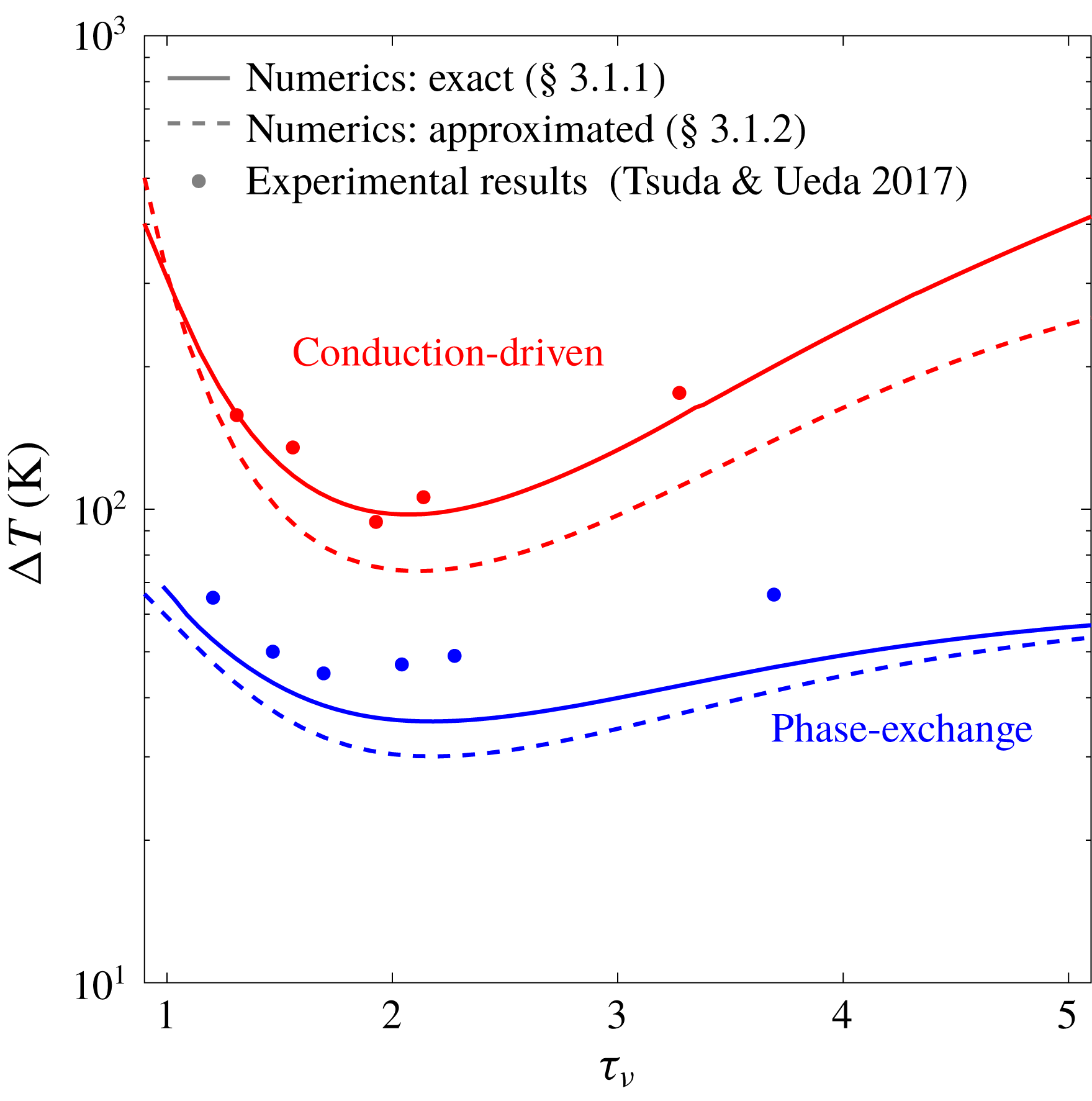
Figure 2. Stability curves for conduction-driven (red) and phase-exchange (blue) thermoacoustic systems, in which the working fluid is air or an air–water mixture, respectively, shown as a function of the Womersley number,
 $\unicode[STIX]{x1D70F}_{\unicode[STIX]{x1D708}}$
. Solid and dashed curves are calculated using the approaches described in § 3.1. All calculations assume ideal sorption (
$\unicode[STIX]{x1D70F}_{\unicode[STIX]{x1D708}}$
. Solid and dashed curves are calculated using the approaches described in § 3.1. All calculations assume ideal sorption (
 $\unicode[STIX]{x1D702}_{\unicode[STIX]{x1D708}}=\unicode[STIX]{x1D702}_{D}=1$
). The mean pressure is
$\unicode[STIX]{x1D702}_{\unicode[STIX]{x1D708}}=\unicode[STIX]{x1D702}_{D}=1$
). The mean pressure is
 $p_{m}=1$
bar, the stack cold-side temperature is
$p_{m}=1$
bar, the stack cold-side temperature is
 $T_{c}=23\,^{\circ }\text{C}$
, and scaled stack length and location are
$T_{c}=23\,^{\circ }\text{C}$
, and scaled stack length and location are
 $L_{s}/L=0.026$
and
$L_{s}/L=0.026$
and
 $L_{0}/L=0.84$
, respectively. Experimental results, marked by filled dots, are taken from Tsuda & Ueda (Reference Tsuda and Ueda2017).
$L_{0}/L=0.84$
, respectively. Experimental results, marked by filled dots, are taken from Tsuda & Ueda (Reference Tsuda and Ueda2017).
First, we compare the two mechanisms of heat transfer, namely conduction and phase exchange. In this comparison, shown in figure 2, we calculated
 $\unicode[STIX]{x0394}T_{onset}$
using the two methods presented in § 3.1 as a function of the Womersley number, here denoted by
$\unicode[STIX]{x0394}T_{onset}$
using the two methods presented in § 3.1 as a function of the Womersley number, here denoted by
 $\unicode[STIX]{x1D70F}_{\unicode[STIX]{x1D708}}$
. The results of conduction-driven thermoacoustics are obtained by setting
$\unicode[STIX]{x1D70F}_{\unicode[STIX]{x1D708}}$
. The results of conduction-driven thermoacoustics are obtained by setting
 $C_{m}\equiv 0$
, reducing the equations to the known form of ‘classical’ thermoacoustics (Rott Reference Rott1969). The experimental results, reported by Tsuda & Ueda (Reference Tsuda and Ueda2017), show good agreement with the theoretical curves. In these experiments the working fluid comprises air and water vapour that evaporate/condense on the stack solid walls, matching the simple case of phase change derived by Raspet et al. (Reference Raspet, Slaton, Hickey and Hiller2002), which in our model corresponds to
$C_{m}\equiv 0$
, reducing the equations to the known form of ‘classical’ thermoacoustics (Rott Reference Rott1969). The experimental results, reported by Tsuda & Ueda (Reference Tsuda and Ueda2017), show good agreement with the theoretical curves. In these experiments the working fluid comprises air and water vapour that evaporate/condense on the stack solid walls, matching the simple case of phase change derived by Raspet et al. (Reference Raspet, Slaton, Hickey and Hiller2002), which in our model corresponds to
 $\unicode[STIX]{x1D702}_{n}=1$
(see § 2.1). This agreement validates our model’s (as well as that of Raspet et al.
Reference Raspet, Slaton, Hickey and Hiller2002) ability to accurately capture the physical mechanisms in both conduction-driven and phase-exchange thermoacoustics.
$\unicode[STIX]{x1D702}_{n}=1$
(see § 2.1). This agreement validates our model’s (as well as that of Raspet et al.
Reference Raspet, Slaton, Hickey and Hiller2002) ability to accurately capture the physical mechanisms in both conduction-driven and phase-exchange thermoacoustics.
Compared with the conduction-driven system, the phase exchange substantially decreases the onset temperature difference. This distinction is best understood comparing the conduction-driven and phase-exchange heat-to-acoustic work terms (see (2.59)). In the limit of ideal sorption, using (3.2) to express
 $\text{d}C_{m}/\text{d}x$
as a function of
$\text{d}C_{m}/\text{d}x$
as a function of
 $\text{d}T_{m}/\text{d}x$
and assuming
$\text{d}T_{m}/\text{d}x$
and assuming
 $Pr\approx Sc$
, these terms differ only by the factor
$Pr\approx Sc$
, these terms differ only by the factor
 $$\begin{eqnarray}\unicode[STIX]{x1D713}\approx \frac{C_{m}}{1-C_{m}}\frac{l_{h}}{RT_{m}},\end{eqnarray}$$
which serves as a ‘booster’ for the temperature gradient, employing it to transfer heat through phase exchange of the reactive gas at the sorbent interface. The term
 $C_{m}/(1-C_{m})$
equals
$C_{m}/(1-C_{m})$
equals
 $1$
for
$1$
for
 $C_{m}=0.5$
and rapidly increases when the reactive gas constitutes more than half of the mixture. The non-dimensional group,
$C_{m}=0.5$
and rapidly increases when the reactive gas constitutes more than half of the mixture. The non-dimensional group,
 $l_{h}/(RT_{m})$
, is typically much larger than
$l_{h}/(RT_{m})$
, is typically much larger than
 $1$
(see table 1). If
$1$
(see table 1). If
 $\unicode[STIX]{x1D713}=1$
the two mechanisms contribute equally (approximately) to the conversion of heat to acoustic work, although choosing an appropriate reactive gas and setting the working conditions to increase
$\unicode[STIX]{x1D713}=1$
the two mechanisms contribute equally (approximately) to the conversion of heat to acoustic work, although choosing an appropriate reactive gas and setting the working conditions to increase
 $C_{m}$
, one may easily achieve
$C_{m}$
, one may easily achieve
 $\unicode[STIX]{x1D713}\gg 1$
. As
$\unicode[STIX]{x1D713}\gg 1$
. As
 $\unicode[STIX]{x1D713}$
increases, more acoustic work is produced for the same temperature gradient or, in our case, onset is reached with a lower temperature difference along the stack.
$\unicode[STIX]{x1D713}$
increases, more acoustic work is produced for the same temperature gradient or, in our case, onset is reached with a lower temperature difference along the stack.
Comparing between the two approaches taken for the stability analysis calculations, we notice the ‘zero acoustic power’ curves lie below their corresponding curves calculated using the numerical scheme. In the finite differences scheme
 $p_{1}(x)$
and
$p_{1}(x)$
and
 $u_{1}(x)$
are the explicit solution to the boundary value problem in (3.3)–(3.4), while in the ‘zero acoustic power’ method these are assumed to obey a pure standing-wave behaviour, independent of
$u_{1}(x)$
are the explicit solution to the boundary value problem in (3.3)–(3.4), while in the ‘zero acoustic power’ method these are assumed to obey a pure standing-wave behaviour, independent of
 $\unicode[STIX]{x1D70F}_{\unicode[STIX]{x1D708}}$
. This ‘ideal wave’ assumption leads to an artificial decrease in
$\unicode[STIX]{x1D70F}_{\unicode[STIX]{x1D708}}$
. This ‘ideal wave’ assumption leads to an artificial decrease in
 $\unicode[STIX]{x0394}T_{onset}$
since the method does not account for all the losses in the system. The better agreement with experimental results confirms the improved accuracy of the numerical scheme over the ‘zero acoustic power’ method.
$\unicode[STIX]{x0394}T_{onset}$
since the method does not account for all the losses in the system. The better agreement with experimental results confirms the improved accuracy of the numerical scheme over the ‘zero acoustic power’ method.
Table 1. Characteristic values of parameters affecting the choice of reactive gas for phase-exchange thermoacoustic systems, shown for water, ethanol and methanol. Values are calculated for a mean pressure
 $p_{m}=1$
bar.
$p_{m}=1$
bar.

Another point worth mentioning is that, while the conduction-driven curves are unbounded, with
 $\unicode[STIX]{x0394}T_{onset}$
tending to infinity for
$\unicode[STIX]{x0394}T_{onset}$
tending to infinity for
 $\unicode[STIX]{x1D70F}_{\unicode[STIX]{x1D708}}\rightarrow 0$
and
$\unicode[STIX]{x1D70F}_{\unicode[STIX]{x1D708}}\rightarrow 0$
and
 $\unicode[STIX]{x1D70F}_{\unicode[STIX]{x1D708}}\rightarrow \infty$
, the temperature in phase-exchange systems is bounded by a ‘depletion temperature’,
$\unicode[STIX]{x1D70F}_{\unicode[STIX]{x1D708}}\rightarrow \infty$
, the temperature in phase-exchange systems is bounded by a ‘depletion temperature’,
 $T_{max}$
, namely the temperature at which the sorbent can no longer sorb gas (or, equivalently, the boiling temperature,
$T_{max}$
, namely the temperature at which the sorbent can no longer sorb gas (or, equivalently, the boiling temperature,
 $T_{b}$
, for a simple phase change process), such that
$T_{b}$
, for a simple phase change process), such that
 $\unicode[STIX]{x0394}T_{onset}\leqslant T_{max}-T_{c}$
. The Clausius–Clapeyron equation, used in our model, relates the partial pressure (in our scaled notation,
$\unicode[STIX]{x0394}T_{onset}\leqslant T_{max}-T_{c}$
. The Clausius–Clapeyron equation, used in our model, relates the partial pressure (in our scaled notation,
 $C_{m}$
) to the temperature for an equilibrium state of saturation. If the fluid temperature surpasses
$C_{m}$
) to the temperature for an equilibrium state of saturation. If the fluid temperature surpasses
 $T_{max}$
, the mean pressure must increase to allow the fluid to remain saturated. In our linear analysis the mean pressure is constant (see § 2.1); if we allow the gas mixture temperature to exceed
$T_{max}$
, the mean pressure must increase to allow the fluid to remain saturated. In our linear analysis the mean pressure is constant (see § 2.1); if we allow the gas mixture temperature to exceed
 $T_{max}$
the reactive gas will no longer be saturated and thus, it cannot condense into a liquid film. This limitation may, in principal, be corrected by extending the model to include
$T_{max}$
the reactive gas will no longer be saturated and thus, it cannot condense into a liquid film. This limitation may, in principal, be corrected by extending the model to include
 $O(\unicode[STIX]{x1D700}^{2})$
terms, thus adding a second-order,
$O(\unicode[STIX]{x1D700}^{2})$
terms, thus adding a second-order,
 $x$
-dependent correction to the mean pressure.
$x$
-dependent correction to the mean pressure.
4.1.2 Effects of mixture composition
We now examine different gas mixture compositions and how their properties affect the temperature difference required for onset. The inert gas in the mixtures is either air or helium, two commonly used gases in thermoacoustic systems (Arnott, Bass & Raspet Reference Arnott, Bass and Raspet1992; Swift Reference Swift1992). The reactive gases selected for this comparison are water, ethanol and methanol, all used as condensable vapours that undergo evaporation/condensation. Accordingly,
 $l_{h}$
is the latent heat of evaporation; for water this value is obtained from steam tables, while for ethanol and methanol it is calculated according to Majer & Svoboda (Reference Majer and Svoboda1985). All other gas mixture properties are calculated using the kinetic theory of gases (Poling, Prausnitz & O’Connell Reference Poling, Prausnitz and O’Connell2001). Characteristic values of the parameters affecting the choice of the reactive gases are listed in table 1.
$l_{h}$
is the latent heat of evaporation; for water this value is obtained from steam tables, while for ethanol and methanol it is calculated according to Majer & Svoboda (Reference Majer and Svoboda1985). All other gas mixture properties are calculated using the kinetic theory of gases (Poling, Prausnitz & O’Connell Reference Poling, Prausnitz and O’Connell2001). Characteristic values of the parameters affecting the choice of the reactive gases are listed in table 1.

Figure 3. Stability curves for gas mixtures employing air (solid lines) and helium (dashed lines) as inert gases. The reactive gases are water (black), ethanol (red) and methanol (blue). The mean pressure is
 $p_{m}=1$
bar, scaled stack length and location are
$p_{m}=1$
bar, scaled stack length and location are
 $L_{s}/L=0.04$
and
$L_{s}/L=0.04$
and
 $L_{0}/L=0.8$
, respectively, and ideal sorption is assumed (
$L_{0}/L=0.8$
, respectively, and ideal sorption is assumed (
 $\unicode[STIX]{x1D702}_{\unicode[STIX]{x1D708}}=\unicode[STIX]{x1D702}_{D}=1$
). Curves are plotted against: (a) the Womersley number,
$\unicode[STIX]{x1D702}_{\unicode[STIX]{x1D708}}=\unicode[STIX]{x1D702}_{D}=1$
). Curves are plotted against: (a) the Womersley number,
 $\unicode[STIX]{x1D70F}_{\unicode[STIX]{x1D708}}\equiv h(\unicode[STIX]{x1D714}/\unicode[STIX]{x1D708})^{1/2}$
, where the stack cold-side temperature is
$\unicode[STIX]{x1D70F}_{\unicode[STIX]{x1D708}}\equiv h(\unicode[STIX]{x1D714}/\unicode[STIX]{x1D708})^{1/2}$
, where the stack cold-side temperature is
 $T_{c}=20\,^{\circ }\text{C}$
, and (b) the averaged concentration of the reactive gas in the stack,
$T_{c}=20\,^{\circ }\text{C}$
, and (b) the averaged concentration of the reactive gas in the stack,
 $\overline{C_{m}}$
, for
$\overline{C_{m}}$
, for
 $\unicode[STIX]{x1D70F}_{\unicode[STIX]{x1D708}}=2.5$
.
$\unicode[STIX]{x1D70F}_{\unicode[STIX]{x1D708}}=2.5$
.
Figure 3(a) presents stability curves of the selected gas mixtures as a function of
 $\unicode[STIX]{x1D70F}_{\unicode[STIX]{x1D708}}$
. Mixtures employing air as the inert gas outperform their matching helium-based mixtures in terms of
$\unicode[STIX]{x1D70F}_{\unicode[STIX]{x1D708}}$
. Mixtures employing air as the inert gas outperform their matching helium-based mixtures in terms of
 $\unicode[STIX]{x0394}T_{onset}$
. A possible explanation is helium’s large heat capacity, compared with that of practically any gas, which requires a larger temperature difference for the same amount of heat to be transferred to the gas through conduction during an oscillation cycle, resulting in higher values of
$\unicode[STIX]{x0394}T_{onset}$
. A possible explanation is helium’s large heat capacity, compared with that of practically any gas, which requires a larger temperature difference for the same amount of heat to be transferred to the gas through conduction during an oscillation cycle, resulting in higher values of
 $\unicode[STIX]{x0394}T_{onset}$
. The closer a mixture is to the reactive component’s boiling temperature, the less dominant this effect is as the reactive gas becomes a larger fraction in the mixture, reflected through the concentration,
$\unicode[STIX]{x0394}T_{onset}$
. The closer a mixture is to the reactive component’s boiling temperature, the less dominant this effect is as the reactive gas becomes a larger fraction in the mixture, reflected through the concentration,
 $C_{m}$
. As
$C_{m}$
. As
 $C_{m}$
increases, more of the gas in the mixture participates in the isothermal phase-exchange heat transfer mechanism, as clearly indicated by the parameter
$C_{m}$
increases, more of the gas in the mixture participates in the isothermal phase-exchange heat transfer mechanism, as clearly indicated by the parameter
 $\unicode[STIX]{x1D713}\propto C_{m}/(1-C_{m})$
(see table 1 for characteristic values). In these calculations, the cold side temperature,
$\unicode[STIX]{x1D713}\propto C_{m}/(1-C_{m})$
(see table 1 for characteristic values). In these calculations, the cold side temperature,
 $T_{c}$
, is fixed at
$T_{c}$
, is fixed at
 $20\,^{\circ }\text{C}$
for all mixtures, resulting in different values of
$20\,^{\circ }\text{C}$
for all mixtures, resulting in different values of
 $C_{m}$
, determined by the proximity of
$C_{m}$
, determined by the proximity of
 $T_{c}$
to the fluid freezing and boiling temperatures. The value of
$T_{c}$
to the fluid freezing and boiling temperatures. The value of
 $T_{c}$
was chosen for practical reasons as it is close to the ambient temperature, making it easier to maintain. While water at
$T_{c}$
was chosen for practical reasons as it is close to the ambient temperature, making it easier to maintain. While water at
 $p_{m}=1$
bar coexists as liquid/vapour between
$p_{m}=1$
bar coexists as liquid/vapour between
 $0<T<100\,^{\circ }\text{C}$
, EtOH and MeOH span a wider temperature range, and their boiling temperatures are significantly lower than that of
$0<T<100\,^{\circ }\text{C}$
, EtOH and MeOH span a wider temperature range, and their boiling temperatures are significantly lower than that of
 $\text{H}_{2}\text{O}$
(see table 1). Accordingly, the values of
$\text{H}_{2}\text{O}$
(see table 1). Accordingly, the values of
 $C_{m}$
in their mixtures for
$C_{m}$
in their mixtures for
 $T_{c}\leqslant T\leqslant T_{b}$
are substantially higher than for water (see table 1 for
$T_{c}\leqslant T\leqslant T_{b}$
are substantially higher than for water (see table 1 for
 $C_{m}$
values at
$C_{m}$
values at
 $T=T_{c}$
), contributing to lower values of
$T=T_{c}$
), contributing to lower values of
 $\unicode[STIX]{x0394}T_{onset}$
.
$\unicode[STIX]{x0394}T_{onset}$
.
The results shown in figure 3(b) compare stability curves of the considered gas mixtures as a function of the averaged concentration of the reactive component in the stack,
 $\overline{C_{m}}$
. The bar in
$\overline{C_{m}}$
. The bar in
 $\overline{C_{m}}$
denotes axial averaging across the stack, and is an exception to its typical use for time averaging. All curves are calculated for
$\overline{C_{m}}$
denotes axial averaging across the stack, and is an exception to its typical use for time averaging. All curves are calculated for
 $\unicode[STIX]{x1D70F}_{\unicode[STIX]{x1D708}}=2.5$
, a value representative of good performance for all mixtures (see figure 3
a). Here, different values of
$\unicode[STIX]{x1D70F}_{\unicode[STIX]{x1D708}}=2.5$
, a value representative of good performance for all mixtures (see figure 3
a). Here, different values of
 $\overline{C_{m}}$
are obtained by setting different temperatures as
$\overline{C_{m}}$
are obtained by setting different temperatures as
 $T_{c}$
, such that the temperatures on the stack are in the range
$T_{c}$
, such that the temperatures on the stack are in the range
 $T_{c}\leqslant T\leqslant T_{b}$
. As
$T_{c}\leqslant T\leqslant T_{b}$
. As
 $T_{c}$
increases this range in narrowed, increasing
$T_{c}$
increases this range in narrowed, increasing
 $\overline{C_{m}}$
, thus decreasing
$\overline{C_{m}}$
, thus decreasing
 $\unicode[STIX]{x0394}T_{onset}$
as the phase-exchange mechanism is more dominant. At a certain point the temperature range narrows to match
$\unicode[STIX]{x0394}T_{onset}$
as the phase-exchange mechanism is more dominant. At a certain point the temperature range narrows to match
 $\unicode[STIX]{x0394}T_{onset}$
, setting the lowest possible temperature difference that would initiate onset, under the considered conditions. For all mixtures presented here the lowest temperature difference is
$\unicode[STIX]{x0394}T_{onset}$
, setting the lowest possible temperature difference that would initiate onset, under the considered conditions. For all mixtures presented here the lowest temperature difference is
 $\unicode[STIX]{x0394}T_{min}\approx 5\,^{\circ }\text{C}$
, with
$\unicode[STIX]{x0394}T_{min}\approx 5\,^{\circ }\text{C}$
, with
 $\overline{C_{m}}\approx 0.85$
.
$\overline{C_{m}}\approx 0.85$
.
At low values of
 $\overline{C_{m}}$
the curves may be separated into two clearly visible groups: air- and helium-based mixtures. This separation is a consequence of the results shown in figure 3(a), where mixtures employing helium as the inert gas exhibited higher values of
$\overline{C_{m}}$
the curves may be separated into two clearly visible groups: air- and helium-based mixtures. This separation is a consequence of the results shown in figure 3(a), where mixtures employing helium as the inert gas exhibited higher values of
 $\unicode[STIX]{x0394}T_{onset}$
. As
$\unicode[STIX]{x0394}T_{onset}$
. As
 $\overline{C_{m}}$
increases, the reactive gas becomes a larger fraction in the mixture, gradually suppressing the differences between the two groups. At the highest concentration values for which onset is reached (
$\overline{C_{m}}$
increases, the reactive gas becomes a larger fraction in the mixture, gradually suppressing the differences between the two groups. At the highest concentration values for which onset is reached (
 $\overline{C_{m}}\approx 0.85$
), all curves appear to converge to the same value. The values of
$\overline{C_{m}}\approx 0.85$
), all curves appear to converge to the same value. The values of
 $\unicode[STIX]{x0394}T_{onset}$
in this case are so low that the temperature gradient imposed on the stack is lower than the adiabatic temperature gradient experienced by the gas as it compresses and expands. Accordingly, the conduction-driven mechanism cannot convert heat to acoustic power, leaving only the phase-exchange mechanism to produce the required acoustic power that triggers the instability. This heat-to-acoustic power conversion is governed by the parameter
$\unicode[STIX]{x0394}T_{onset}$
in this case are so low that the temperature gradient imposed on the stack is lower than the adiabatic temperature gradient experienced by the gas as it compresses and expands. Accordingly, the conduction-driven mechanism cannot convert heat to acoustic power, leaving only the phase-exchange mechanism to produce the required acoustic power that triggers the instability. This heat-to-acoustic power conversion is governed by the parameter
 $\unicode[STIX]{x1D713}$
, dependent on
$\unicode[STIX]{x1D713}$
, dependent on
 $C_{m}$
,
$C_{m}$
,
 $T_{m}$
and the reactive gas latent heat,
$T_{m}$
and the reactive gas latent heat,
 $l_{h}$
. Here
$l_{h}$
. Here
 $\overline{C_{m}}$
is practically equal for all mixtures, leaving the non-dimensional group
$\overline{C_{m}}$
is practically equal for all mixtures, leaving the non-dimensional group
 $l_{h}/(RT_{m})$
to distinguish between the gas mixtures and their performance. As
$l_{h}/(RT_{m})$
to distinguish between the gas mixtures and their performance. As
 $C_{m}$
on the stack is close to
$C_{m}$
on the stack is close to
 $1$
, all temperatures are very close to the reactive component’s boiling temperature,
$1$
, all temperatures are very close to the reactive component’s boiling temperature,
 $T_{b}$
, such that
$T_{b}$
, such that
 $\unicode[STIX]{x1D713}$
may be approximated as
$\unicode[STIX]{x1D713}$
may be approximated as
 $$\begin{eqnarray}\unicode[STIX]{x1D713}\approx \frac{0.85}{1-0.85}\frac{l_{h}}{RT_{b}},\end{eqnarray}$$
where
 $\overline{C_{m}}\approx 0.85$
is the value for which
$\overline{C_{m}}\approx 0.85$
is the value for which
 $\unicode[STIX]{x0394}T_{min}$
is obtained. The non-dimensional group
$\unicode[STIX]{x0394}T_{min}$
is obtained. The non-dimensional group
 $l_{h}/(RT_{b})$
displays similar values for all three reactive gases chosen (see table 1). As a result, all mixtures converge to a very similar value of
$l_{h}/(RT_{b})$
displays similar values for all three reactive gases chosen (see table 1). As a result, all mixtures converge to a very similar value of
 $\unicode[STIX]{x0394}T_{min}$
, although slight changes in
$\unicode[STIX]{x0394}T_{min}$
, although slight changes in
 $\unicode[STIX]{x0394}T_{min}$
between the different mixtures are perceptible. These changes may be explained by the factor
$\unicode[STIX]{x0394}T_{min}$
between the different mixtures are perceptible. These changes may be explained by the factor
 $1/T_{m}$
multiplying
$1/T_{m}$
multiplying
 $\unicode[STIX]{x1D713}$
in the phase-exchange heat-to-acoustic work term, which may also be approximated as
$\unicode[STIX]{x1D713}$
in the phase-exchange heat-to-acoustic work term, which may also be approximated as
 $1/T_{m}\approx 1/T_{b}$
. The small variations in the values of
$1/T_{m}\approx 1/T_{b}$
. The small variations in the values of
 $l_{h}/(RT_{b}^{2})$
for the three gases, listed in table 1, are reflected in the values of
$l_{h}/(RT_{b}^{2})$
for the three gases, listed in table 1, are reflected in the values of
 $\unicode[STIX]{x0394}T_{min}$
seen in figure 3(b).
$\unicode[STIX]{x0394}T_{min}$
seen in figure 3(b).
4.1.3 Sorption kinetics

Figure 4. Stability curves for an air–water gas mixture at various values of the partition coefficient
 $K$
, as a function of the kinetics non-dimensional number,
$K$
, as a function of the kinetics non-dimensional number,
 $R_{k}$
. The mean pressure is
$R_{k}$
. The mean pressure is
 $p_{m}=1$
bar, the Womersley number is
$p_{m}=1$
bar, the Womersley number is
 $\unicode[STIX]{x1D70F}_{\unicode[STIX]{x1D708}}=2.5$
, and scaled stack length and location are
$\unicode[STIX]{x1D70F}_{\unicode[STIX]{x1D708}}=2.5$
, and scaled stack length and location are
 $L_{s}/L=0.03$
and
$L_{s}/L=0.03$
and
 $L_{0}/L=0.8$
, respectively.
$L_{0}/L=0.8$
, respectively.
The curves presented in figure 4 examine effects of reaction kinetics in a sorption process, where
 $\unicode[STIX]{x1D702}_{\unicode[STIX]{x1D708}},\unicode[STIX]{x1D702}_{D}\neq 1$
. These stability curves, calculated for different values of the partition coefficient
$\unicode[STIX]{x1D702}_{\unicode[STIX]{x1D708}},\unicode[STIX]{x1D702}_{D}\neq 1$
. These stability curves, calculated for different values of the partition coefficient
 $K$
, are plotted against
$K$
, are plotted against
 $R_{k}\equiv \unicode[STIX]{x1D708}/(h^{2}k_{d})$
, a non-dimensional number linking the characteristic viscous and desorption time scales such that
$R_{k}\equiv \unicode[STIX]{x1D708}/(h^{2}k_{d})$
, a non-dimensional number linking the characteristic viscous and desorption time scales such that
 $\unicode[STIX]{x1D70F}_{k}\equiv \sqrt{R_{k}}\unicode[STIX]{x1D70F}_{\unicode[STIX]{x1D708}}$
. All curves are calculated for an air–water mixture.
$\unicode[STIX]{x1D70F}_{k}\equiv \sqrt{R_{k}}\unicode[STIX]{x1D70F}_{\unicode[STIX]{x1D708}}$
. All curves are calculated for an air–water mixture.
 $R_{k}\rightarrow 0$
and
$R_{k}\rightarrow 0$
and
 $R_{k}\rightarrow \infty$
denote the limits of fast and slow kinetics relative to the oscillation time scale, respectively. The dashed lines represent the two extreme cases for the sorbent/sorbate pair: ‘ideal’ sorption (
$R_{k}\rightarrow \infty$
denote the limits of fast and slow kinetics relative to the oscillation time scale, respectively. The dashed lines represent the two extreme cases for the sorbent/sorbate pair: ‘ideal’ sorption (
 $K\rightarrow \infty$
), in which the sorbent has no limitation on its capacity for sorbing gas (also applicable for evaporation/condensation from/to a liquid film, unbounded in its capacity for condensed vapour – see § 2.2), and no sorption (
$K\rightarrow \infty$
), in which the sorbent has no limitation on its capacity for sorbing gas (also applicable for evaporation/condensation from/to a liquid film, unbounded in its capacity for condensed vapour – see § 2.2), and no sorption (
 $K\rightarrow 0$
), where the sorbent has zero capacity for sorbing the reactive gas such that (2.58) is reduced to the conduction-driven form (Rott Reference Rott1969). All the curves approach the limit of
$K\rightarrow 0$
), where the sorbent has zero capacity for sorbing the reactive gas such that (2.58) is reduced to the conduction-driven form (Rott Reference Rott1969). All the curves approach the limit of
 $K\rightarrow 0$
for vanishingly slow kinetics (very large values of
$K\rightarrow 0$
for vanishingly slow kinetics (very large values of
 $R_{k}$
), where the oscillations are too fast to allow mass exchange at the sorbent interface. In the case of fast kinetics, sorption occurs instantly, resulting in a quasi-steady state of equilibrium between the sorbent and gas phases. Accordingly, at low values of
$R_{k}$
), where the oscillations are too fast to allow mass exchange at the sorbent interface. In the case of fast kinetics, sorption occurs instantly, resulting in a quasi-steady state of equilibrium between the sorbent and gas phases. Accordingly, at low values of
 $R_{k}$
all curves flatten towards a specific value, determined by the partition coefficient,
$R_{k}$
all curves flatten towards a specific value, determined by the partition coefficient,
 $K$
, specifying the sorbent capacity for sorbing the reactive gas. If
$K$
, specifying the sorbent capacity for sorbing the reactive gas. If
 $K$
surpasses a certain value, here
$K$
surpasses a certain value, here
 $K\approx 10^{-2}$
, all curves are monotonically increasing, with the ascent towards the horizontal asymptote of
$K\approx 10^{-2}$
, all curves are monotonically increasing, with the ascent towards the horizontal asymptote of
 $K\rightarrow 0$
occurring at different values of
$K\rightarrow 0$
occurring at different values of
 $R_{k}$
. A curious limit is obtained for the case of ideal sorption occurring at an infinitesimally slow rate, for which the kinetics parameter does not recover
$R_{k}$
. A curious limit is obtained for the case of ideal sorption occurring at an infinitesimally slow rate, for which the kinetics parameter does not recover
 $\unicode[STIX]{x1D702}_{n}\rightarrow 1$
nor
$\unicode[STIX]{x1D702}_{n}\rightarrow 1$
nor
 $\unicode[STIX]{x1D702}_{n}\rightarrow \infty$
, but rather an intermediate result, unaffected by the reaction rate and strongly dependent on the parameters
$\unicode[STIX]{x1D702}_{n}\rightarrow \infty$
, but rather an intermediate result, unaffected by the reaction rate and strongly dependent on the parameters
 $\unicode[STIX]{x1D6EC}$
and
$\unicode[STIX]{x1D6EC}$
and
 $N^{s}$
, characterising the sorbent/sorbate pair.
$N^{s}$
, characterising the sorbent/sorbate pair.
While large values of
 $K$
result in monotonically increasing curves, small values of
$K$
result in monotonically increasing curves, small values of
 $K$
clearly show a minimum at
$K$
clearly show a minimum at
 $R_{k}\approx 10^{-1}$
. Intuitively, one may assume the lowest temperature difference is always recovered for the limit of fast kinetics. For small
$R_{k}\approx 10^{-1}$
. Intuitively, one may assume the lowest temperature difference is always recovered for the limit of fast kinetics. For small
 $K$
values, however, the sorbent has very limited capacity for sorption, such that for
$K$
values, however, the sorbent has very limited capacity for sorption, such that for
 $R_{k}\rightarrow 0$
mass exchange occurs in only a very small fraction of an oscillation cycle. During the remainder of the cycle, then, the sorbent is saturated and the phase-exchange mechanism is not active, resulting in an increase in
$R_{k}\rightarrow 0$
mass exchange occurs in only a very small fraction of an oscillation cycle. During the remainder of the cycle, then, the sorbent is saturated and the phase-exchange mechanism is not active, resulting in an increase in
 $\unicode[STIX]{x0394}T_{onset}$
as
$\unicode[STIX]{x0394}T_{onset}$
as
 $K$
decreases. An intentional, moderate increase in
$K$
decreases. An intentional, moderate increase in
 $R_{k}$
, namely a regulated delay in desorption rate, allows the sorbent to exchange mass with the gas mixture during a larger fraction of the oscillation cycle, thus lengthening the characteristic time in which the phase-exchange mechanism is active and consequently decreasing
$R_{k}$
, namely a regulated delay in desorption rate, allows the sorbent to exchange mass with the gas mixture during a larger fraction of the oscillation cycle, thus lengthening the characteristic time in which the phase-exchange mechanism is active and consequently decreasing
 $\unicode[STIX]{x0394}T_{onset}$
.
$\unicode[STIX]{x0394}T_{onset}$
.
4.2 Limit cycle analysis
In this section we analyse the limit cycle of a phase-exchange system, i.e. the state at which the amplitude of oscillating quantities ‘saturates’ and becomes constant, typically obtained for
 $t\gg t_{onset}$
, where
$t\gg t_{onset}$
, where
 $t_{onset}$
marks the stability limit breaching point in time. All results are calculated for an air–water mixture. Unless otherwise stated, the scaled stack length and location are
$t_{onset}$
marks the stability limit breaching point in time. All results are calculated for an air–water mixture. Unless otherwise stated, the scaled stack length and location are
 $L_{s}/L=0.04$
and
$L_{s}/L=0.04$
and
 $L_{0}/L=0.83$
, respectively, the limit of ideal sorption (
$L_{0}/L=0.83$
, respectively, the limit of ideal sorption (
 $\unicode[STIX]{x1D702}_{\unicode[STIX]{x1D708}}=\unicode[STIX]{x1D702}_{D}=1$
) is assumed, and the heat flux input to the system is
$\unicode[STIX]{x1D702}_{\unicode[STIX]{x1D708}}=\unicode[STIX]{x1D702}_{D}=1$
) is assumed, and the heat flux input to the system is
 $Q_{h}=25~\text{kW}~\text{m}^{-2}$
.
$Q_{h}=25~\text{kW}~\text{m}^{-2}$
.
4.2.1 Acoustic field characteristics
In the considered system configuration (shown in figure 1 a) the no-penetration boundary conditions at the two closed ends impose a near-standing-wave behaviour of pressure and velocity. Viscous dissipation at the solid boundaries, the presence of a stack and its asymmetric location within the tube all contribute to a slight distortion of the wave form, deviating from a standing wave, and thus allowing the production (or dissipation) of non-zero acoustic power. However, this deviation is normally very small in standing-wave systems (such as the one considered here, see figure 1 a), and the acoustic power flux
 $$\begin{eqnarray}{\dot{W}}={\textstyle \frac{1}{2}}\text{Re}[\widetilde{p_{1}}u_{1}]={\textstyle \frac{1}{2}}|p_{1}|\,|u_{1}|\cos (\unicode[STIX]{x1D719})\end{eqnarray}$$
is largely dependent on the phase angle between
 $p_{1}$
and
$p_{1}$
and
 $u_{1}$
,
$u_{1}$
,
 $\unicode[STIX]{x1D719}$
, which is typically in the range
$\unicode[STIX]{x1D719}$
, which is typically in the range
 $|\unicode[STIX]{x1D719}|=90^{\circ }\pm 5^{\circ }$
(Swift Reference Swift1992).
$|\unicode[STIX]{x1D719}|=90^{\circ }\pm 5^{\circ }$
(Swift Reference Swift1992).
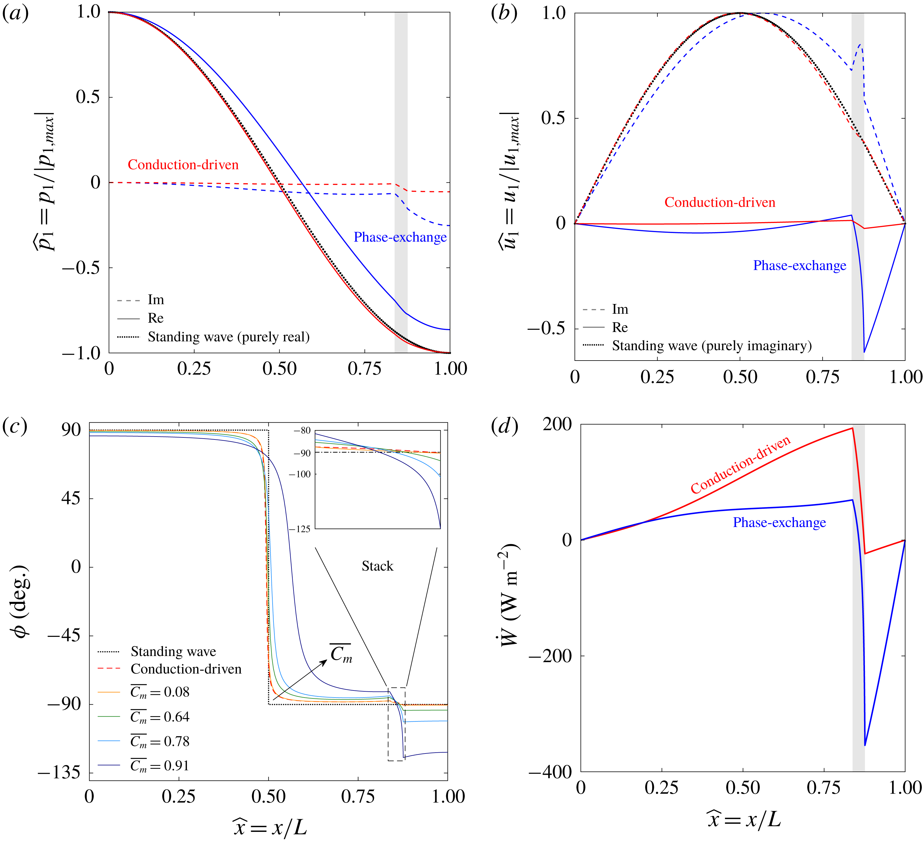
Figure 5. Acoustic field characteristics for conduction-driven (red) and phase-exchange (blue) systems, compared to a pure standing wave (black, dotted): (a) real (solid line) and imaginary (dashed line) components of the pressure amplitude, scaled by the maximum pressure in the system, (b) real (solid line) and imaginary (dashed line) components of the velocity amplitude, scaled by the maximum velocity in the system, (c) phase angle between pressure and velocity,
 $\unicode[STIX]{x1D719}$
, throughout the system, and in the stack in particular (inset), for different mean concentrations of the reactive gas,
$\unicode[STIX]{x1D719}$
, throughout the system, and in the stack in particular (inset), for different mean concentrations of the reactive gas,
 $\overline{C_{m}}$
, and (d) acoustic power. The highest
$\overline{C_{m}}$
, and (d) acoustic power. The highest
 $\overline{C_{m}}$
value presented in (c) corresponds to the phase-exchange curves in (a,b,d). All properties are drawn against
$\overline{C_{m}}$
value presented in (c) corresponds to the phase-exchange curves in (a,b,d). All properties are drawn against
 $\widehat{x}=x/L$
, the axial coordinate scaled by the system length. The shaded area marks the stack location in the system. The mean pressure is
$\widehat{x}=x/L$
, the axial coordinate scaled by the system length. The shaded area marks the stack location in the system. The mean pressure is
 $p_{m}=1$
bar,
$p_{m}=1$
bar,
 $\unicode[STIX]{x1D70F}_{\unicode[STIX]{x1D708}}=2$
, the scaled stack length and location are
$\unicode[STIX]{x1D70F}_{\unicode[STIX]{x1D708}}=2$
, the scaled stack length and location are
 $L_{s}/L=0.04$
and
$L_{s}/L=0.04$
and
 $L_{0}/L=0.83$
, respectively, the heat flux input is
$L_{0}/L=0.83$
, respectively, the heat flux input is
 $Q_{h}=25~\text{kW}~\text{m}^{-2}$
, and ideal sorption is assumed (
$Q_{h}=25~\text{kW}~\text{m}^{-2}$
, and ideal sorption is assumed (
 $\unicode[STIX]{x1D702}_{\unicode[STIX]{x1D708}}=\unicode[STIX]{x1D702}_{D}=1$
).
$\unicode[STIX]{x1D702}_{\unicode[STIX]{x1D708}}=\unicode[STIX]{x1D702}_{D}=1$
).
Figures 5(a) and 5(b) present the axial distribution of pressure and velocity, respectively, in conduction-driven (red) and phase-exchange (blue) systems. Each curve is scaled by its respective maximum value, allowing a clear, visual comparison of the wave forms. For reference, we added curves of a pure standing wave (black, dotted), where
 $p_{1}$
and
$p_{1}$
and
 $u_{1}$
simply obey cosine and sine functions, respectively (see § 3.1.2). In both figures, the conduction-driven curves only slightly deviate from the standing-wave curves; the largest deviation is unsurprisingly spotted in the stack, where acoustic oscillations are enhanced. The phase-exchange curves, calculated for a large value of the ‘reactive’ gas concentration (
$u_{1}$
simply obey cosine and sine functions, respectively (see § 3.1.2). In both figures, the conduction-driven curves only slightly deviate from the standing-wave curves; the largest deviation is unsurprisingly spotted in the stack, where acoustic oscillations are enhanced. The phase-exchange curves, calculated for a large value of the ‘reactive’ gas concentration (
 $\overline{C_{m}}=0.91$
) to demonstrate the magnitude of the effect, deviate strongly from the standing-wave curves. While in conduction-driven systems the stack may be thought of as an acoustic power point source, amplifying random displacements of gas parcels, in phase-exchange systems it also acts as a mass point source. The periodic mass exchange with the sorbent layer draws/releases mass from/to the gas mixture, consequently increasing the reactive gas mass flux in the stack, which translates directly to a sharp increase in velocity (both real and imaginary), seen clearly in figure 5(b) at
$\overline{C_{m}}=0.91$
) to demonstrate the magnitude of the effect, deviate strongly from the standing-wave curves. While in conduction-driven systems the stack may be thought of as an acoustic power point source, amplifying random displacements of gas parcels, in phase-exchange systems it also acts as a mass point source. The periodic mass exchange with the sorbent layer draws/releases mass from/to the gas mixture, consequently increasing the reactive gas mass flux in the stack, which translates directly to a sharp increase in velocity (both real and imaginary), seen clearly in figure 5(b) at
 $\widehat{x}\approx 0.83$
. The asymmetric location of the stack within the system shifts the imaginary component, quasi-sinusoidal velocity distribution towards the stack, where the velocity increases. As a result, the pressure distribution is also shifted from its quasi-cosine profile, and the absolute value of the pressure at the two closed ends clearly shows
$\widehat{x}\approx 0.83$
. The asymmetric location of the stack within the system shifts the imaginary component, quasi-sinusoidal velocity distribution towards the stack, where the velocity increases. As a result, the pressure distribution is also shifted from its quasi-cosine profile, and the absolute value of the pressure at the two closed ends clearly shows
 $|p_{1}(\widehat{x}=0)|>|p_{1}(\widehat{x}=1)|$
, corresponding to the increase in velocity near
$|p_{1}(\widehat{x}=0)|>|p_{1}(\widehat{x}=1)|$
, corresponding to the increase in velocity near
 $\widehat{x}=1$
.
$\widehat{x}=1$
.
Figure 5(c) shows the phase angle between
 $p_{1}$
and
$p_{1}$
and
 $u_{1}$
along the system, for several values of
$u_{1}$
along the system, for several values of
 $\overline{C_{m}}$
, the mean concentration of the reactive gas in the stack. As in figures 5(a) and 5(b), a pure standing-wave curve (black, dotted) and conduction-driven (red, dashed) curves are drawn for comparison. The inset displays a close-up view of the stack, where the phase angle changes rapidly. As reflected from the results of figure 5(a,b), the conduction-driven curve only slightly deviates from the standing-wave curve. In fact, the largest deviation, neglecting the sharp decrease near
$\overline{C_{m}}$
, the mean concentration of the reactive gas in the stack. As in figures 5(a) and 5(b), a pure standing-wave curve (black, dotted) and conduction-driven (red, dashed) curves are drawn for comparison. The inset displays a close-up view of the stack, where the phase angle changes rapidly. As reflected from the results of figure 5(a,b), the conduction-driven curve only slightly deviates from the standing-wave curve. In fact, the largest deviation, neglecting the sharp decrease near
 $\widehat{x}=0.5$
(where the pressure moves from leading the velocity to trailing it), is only
$\widehat{x}=0.5$
(where the pressure moves from leading the velocity to trailing it), is only
 $2.4^{\circ }$
. At the lowest concentration considered (
$2.4^{\circ }$
. At the lowest concentration considered (
 $\overline{C_{m}}=0.08$
), the phase-exchange case is nearly identical to the conduction-driven curve. At such a low concentration, altering the working gas contributes merely to a decrease in the temperature difference along the stack (discussed in § 4.2.2), while the wave form is left unaffected. As
$\overline{C_{m}}=0.08$
), the phase-exchange case is nearly identical to the conduction-driven curve. At such a low concentration, altering the working gas contributes merely to a decrease in the temperature difference along the stack (discussed in § 4.2.2), while the wave form is left unaffected. As
 $\overline{C_{m}}$
is increased, the phase angle distribution departs from the standing-wave behaviour, until at
$\overline{C_{m}}$
is increased, the phase angle distribution departs from the standing-wave behaviour, until at
 $\overline{C_{m}}=0.91$
a remarkable
$\overline{C_{m}}=0.91$
a remarkable
 $35^{\circ }$
deviation from a pure standing wave (
$35^{\circ }$
deviation from a pure standing wave (
 $\unicode[STIX]{x1D719}=-125^{\circ }$
) is obtained at the stack hot end. This difference in phase angles between the conduction-driven and phase-exchange mechanisms translates into an increase in acoustic power, as shown in figure 5(d) (calculated using (4.3)). Although the absolute pressure amplitudes decrease as
$\unicode[STIX]{x1D719}=-125^{\circ }$
) is obtained at the stack hot end. This difference in phase angles between the conduction-driven and phase-exchange mechanisms translates into an increase in acoustic power, as shown in figure 5(d) (calculated using (4.3)). Although the absolute pressure amplitudes decrease as
 $\overline{C_{m}}$
increases (not visible in figure 5
a due to scaling; discussed in § 4.2.2), the dramatic increase in phase angle leads to a higher acoustic power produced by the phase-exchange system.
$\overline{C_{m}}$
increases (not visible in figure 5
a due to scaling; discussed in § 4.2.2), the dramatic increase in phase angle leads to a higher acoustic power produced by the phase-exchange system.
4.2.2 Temperature difference and pressure amplitude
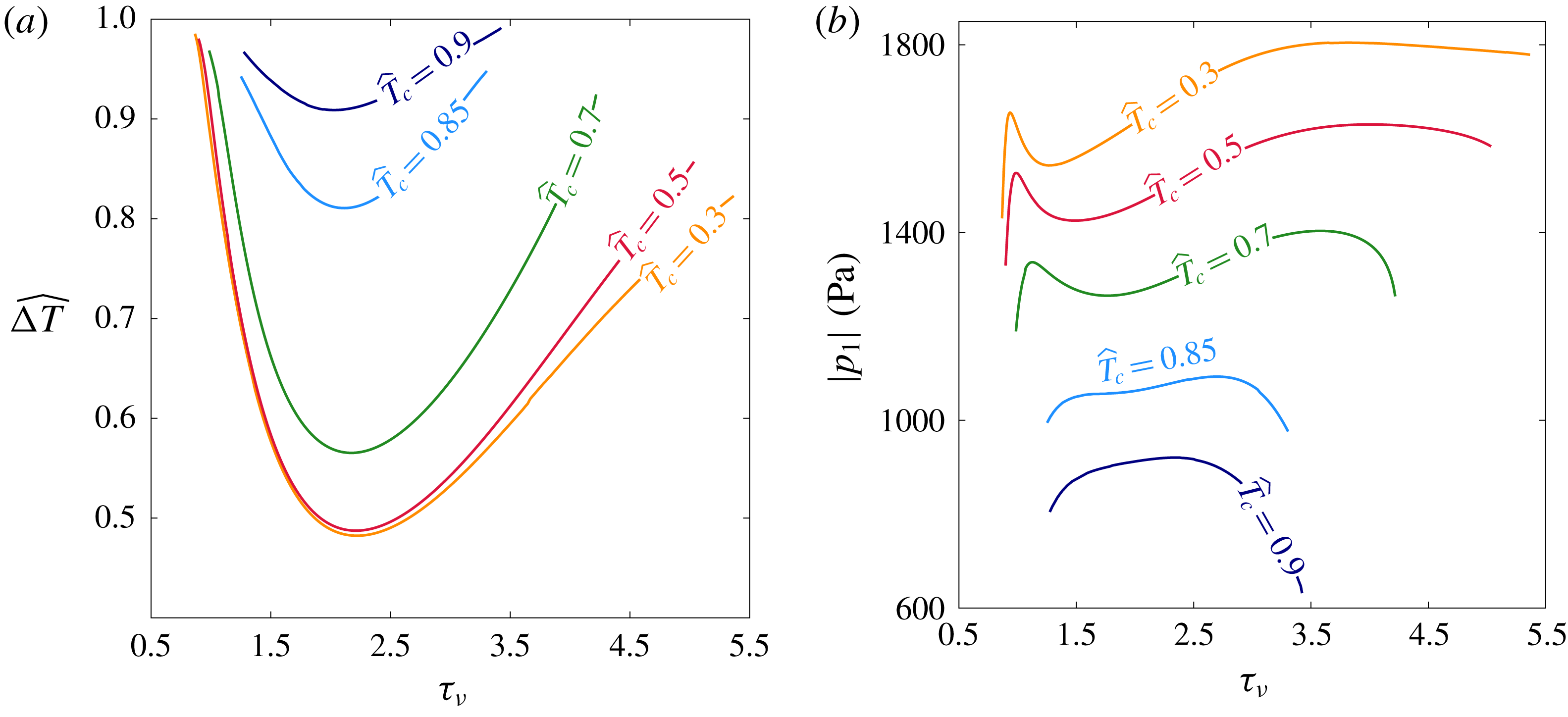
Figure 6. Limit cycle scaled temperature difference across the stack (a) and maximum pressure amplitude (b) as a function of the Womersley number,
 $\unicode[STIX]{x1D70F}_{\unicode[STIX]{x1D708}}$
, for different scaled cold side temperatures,
$\unicode[STIX]{x1D70F}_{\unicode[STIX]{x1D708}}$
, for different scaled cold side temperatures,
 $\widehat{T_{c}}=(T_{c}-T_{min})/(T_{max}-T_{min})$
. The mean pressure is
$\widehat{T_{c}}=(T_{c}-T_{min})/(T_{max}-T_{min})$
. The mean pressure is
 $p_{m}=1$
bar, the scaled stack length and location are
$p_{m}=1$
bar, the scaled stack length and location are
 $L_{s}/L=0.04$
and
$L_{s}/L=0.04$
and
 $L_{0}/L=0.83$
, respectively, the heat flux input is
$L_{0}/L=0.83$
, respectively, the heat flux input is
 $Q_{h}=25~\text{kW}~\text{m}^{-2}$
and ideal sorption is assumed (
$Q_{h}=25~\text{kW}~\text{m}^{-2}$
and ideal sorption is assumed (
 $\unicode[STIX]{x1D702}_{\unicode[STIX]{x1D708}}=\unicode[STIX]{x1D702}_{D}=1$
).
$\unicode[STIX]{x1D702}_{\unicode[STIX]{x1D708}}=\unicode[STIX]{x1D702}_{D}=1$
).
Here, we calculate the temperature difference across the stack and the maximum pressure amplitude (
 $\unicode[STIX]{x0394}T$
and
$\unicode[STIX]{x0394}T$
and
 $|p_{1}|$
, respectively), so as to establish a more complete description of the system limit cycle. Figure 6(a,b) presents these two quantities as a function of the Womersley number,
$|p_{1}|$
, respectively), so as to establish a more complete description of the system limit cycle. Figure 6(a,b) presents these two quantities as a function of the Womersley number,
 $\unicode[STIX]{x1D70F}_{\unicode[STIX]{x1D708}}$
. For each calculation, the boundary condition for the stack cold side temperature,
$\unicode[STIX]{x1D70F}_{\unicode[STIX]{x1D708}}$
. For each calculation, the boundary condition for the stack cold side temperature,
 $T_{c}$
, is varied. For the sake of even comparison, both the cold-side temperature and the temperature difference on the stack are scaled as follows
$T_{c}$
, is varied. For the sake of even comparison, both the cold-side temperature and the temperature difference on the stack are scaled as follows
 $$\begin{eqnarray}\widehat{T_{c}}=\frac{T_{c}-T_{min}}{T_{max}-T_{min}},\quad \widehat{\unicode[STIX]{x0394}T}=\frac{\unicode[STIX]{x0394}T}{T_{max}-T_{c}},\end{eqnarray}$$
where
 $T_{max}$
is the reactive fluid ‘depletion temperature’ (see § 4.1.1), and
$T_{max}$
is the reactive fluid ‘depletion temperature’ (see § 4.1.1), and
 $T_{min}$
is its triple-point temperature, below which the reactive gas component is completely in the sorbed phase and
$T_{min}$
is its triple-point temperature, below which the reactive gas component is completely in the sorbed phase and
 $C_{m}=0$
. For the case of simple phase change through evaporation/condensation
$C_{m}=0$
. For the case of simple phase change through evaporation/condensation
 $T_{min}$
is simply the freezing temperature. The shape of the curves in figure 6(a) resembles that of the stability curves in figures 2 and 3(a): each curve has a unique
$T_{min}$
is simply the freezing temperature. The shape of the curves in figure 6(a) resembles that of the stability curves in figures 2 and 3(a): each curve has a unique
 $\unicode[STIX]{x1D70F}_{\unicode[STIX]{x1D708}}$
value, for which the limit cycle temperature difference is minimised. Here
$\unicode[STIX]{x1D70F}_{\unicode[STIX]{x1D708}}$
value, for which the limit cycle temperature difference is minimised. Here
 $\unicode[STIX]{x1D70F}_{\unicode[STIX]{x1D708}}\approx 2$
marks the minimum in all curves, a representative result for a standing-wave system (Swift Reference Swift2002). When
$\unicode[STIX]{x1D70F}_{\unicode[STIX]{x1D708}}\approx 2$
marks the minimum in all curves, a representative result for a standing-wave system (Swift Reference Swift2002). When
 $\unicode[STIX]{x1D70F}_{D}\equiv \unicode[STIX]{x1D70F}_{\unicode[STIX]{x1D708}}Sc^{1/2}$
, the ratio of the characteristic time scales for molecular diffusion and acoustic oscillations is either too small or too large,
$\unicode[STIX]{x1D70F}_{D}\equiv \unicode[STIX]{x1D70F}_{\unicode[STIX]{x1D708}}Sc^{1/2}$
, the ratio of the characteristic time scales for molecular diffusion and acoustic oscillations is either too small or too large,
 $\unicode[STIX]{x0394}T$
increases, so as to compensate for the poor match between these time scales.
$\unicode[STIX]{x0394}T$
increases, so as to compensate for the poor match between these time scales.
The asymmetric increase in
 $\widehat{\unicode[STIX]{x0394}T}$
for
$\widehat{\unicode[STIX]{x0394}T}$
for
 $\unicode[STIX]{x1D70F}_{\unicode[STIX]{x1D708}}<2$
and
$\unicode[STIX]{x1D70F}_{\unicode[STIX]{x1D708}}<2$
and
 $\unicode[STIX]{x1D70F}_{\unicode[STIX]{x1D708}}>2$
is a result of the match between
$\unicode[STIX]{x1D70F}_{\unicode[STIX]{x1D708}}>2$
is a result of the match between
 $\unicode[STIX]{x1D70F}_{D}$
and the system travelling-wave component, manifested by the deviation of the wave form from that of a pure standing wave,
$\unicode[STIX]{x1D70F}_{D}$
and the system travelling-wave component, manifested by the deviation of the wave form from that of a pure standing wave,
 $$\begin{eqnarray}\unicode[STIX]{x1D703}=||\unicode[STIX]{x1D719}|-90^{\circ }|.\end{eqnarray}$$
In a pure travelling-wave system, perfect thermal contact of the working gas with the boundary is required, i.e.
 $\unicode[STIX]{x1D70F}_{\unicode[STIX]{x1D708}},\unicode[STIX]{x1D70F}_{\unicode[STIX]{x1D6FC}},\unicode[STIX]{x1D70F}_{D}\ll 1$
(Swift Reference Swift2002). For a given
$\unicode[STIX]{x1D70F}_{\unicode[STIX]{x1D708}},\unicode[STIX]{x1D70F}_{\unicode[STIX]{x1D6FC}},\unicode[STIX]{x1D70F}_{D}\ll 1$
(Swift Reference Swift2002). For a given
 $\widehat{T_{c}}$
, as
$\widehat{T_{c}}$
, as
 $\widehat{\unicode[STIX]{x0394}T}$
increases so does
$\widehat{\unicode[STIX]{x0394}T}$
increases so does
 $\overline{C_{m}}$
, subsequently increasing
$\overline{C_{m}}$
, subsequently increasing
 $\unicode[STIX]{x1D703}$
. For
$\unicode[STIX]{x1D703}$
. For
 $\unicode[STIX]{x1D70F}_{\unicode[STIX]{x1D708}}<2$
, the increased
$\unicode[STIX]{x1D70F}_{\unicode[STIX]{x1D708}}<2$
, the increased
 $\unicode[STIX]{x1D703}$
favours the decrease in
$\unicode[STIX]{x1D703}$
favours the decrease in
 $\unicode[STIX]{x1D70F}_{\unicode[STIX]{x1D708}}$
and the system sustains a limit cycle until
$\unicode[STIX]{x1D70F}_{\unicode[STIX]{x1D708}}$
and the system sustains a limit cycle until
 $\widehat{\unicode[STIX]{x0394}T}$
nearly approaches
$\widehat{\unicode[STIX]{x0394}T}$
nearly approaches
 $1$
, marking its highest possible temperature difference. For
$1$
, marking its highest possible temperature difference. For
 $\unicode[STIX]{x1D70F}_{\unicode[STIX]{x1D708}}>2$
each curve reaches a different
$\unicode[STIX]{x1D70F}_{\unicode[STIX]{x1D708}}>2$
each curve reaches a different
 $\widehat{\unicode[STIX]{x0394}T}$
before a limit cycle is no longer sustained at the given heat input. Each
$\widehat{\unicode[STIX]{x0394}T}$
before a limit cycle is no longer sustained at the given heat input. Each
 $\widehat{T_{c}}$
value corresponds to a characteristic
$\widehat{T_{c}}$
value corresponds to a characteristic
 $\overline{C_{m}}$
value, to which a specific
$\overline{C_{m}}$
value, to which a specific
 $\unicode[STIX]{x1D703}$
matches. At
$\unicode[STIX]{x1D703}$
matches. At
 $\widehat{T_{c}}=0.3{-}0.7$
,
$\widehat{T_{c}}=0.3{-}0.7$
,
 $\unicode[STIX]{x1D703}$
is relatively small and, while the curves depart from their optimal standing-wave point (
$\unicode[STIX]{x1D703}$
is relatively small and, while the curves depart from their optimal standing-wave point (
 $\unicode[STIX]{x1D70F}_{\unicode[STIX]{x1D708}}\approx 2$
), the moderate increase in
$\unicode[STIX]{x1D70F}_{\unicode[STIX]{x1D708}}\approx 2$
), the moderate increase in
 $\unicode[STIX]{x1D703}$
does not favour the increase in
$\unicode[STIX]{x1D703}$
does not favour the increase in
 $\unicode[STIX]{x1D70F}_{\unicode[STIX]{x1D708}}$
, and a limit cycle cannot be sustained before
$\unicode[STIX]{x1D70F}_{\unicode[STIX]{x1D708}}$
, and a limit cycle cannot be sustained before
 $\widehat{\unicode[STIX]{x0394}T}$
approaches 1. At
$\widehat{\unicode[STIX]{x0394}T}$
approaches 1. At
 $\widehat{T_{c}}>0.85$
,
$\widehat{T_{c}}>0.85$
,
 $\unicode[STIX]{x1D703}$
is initially large and the curves do not deviate substantially from
$\unicode[STIX]{x1D703}$
is initially large and the curves do not deviate substantially from
 $\unicode[STIX]{x1D70F}_{\unicode[STIX]{x1D708}}=2$
. As
$\unicode[STIX]{x1D70F}_{\unicode[STIX]{x1D708}}=2$
. As
 $\widehat{\unicode[STIX]{x0394}T}$
increases, the increase in
$\widehat{\unicode[STIX]{x0394}T}$
increases, the increase in
 $\unicode[STIX]{x1D703}$
dramatically decreases the resonant frequency (discussed in § 4.2.3), thus reducing the system losses – proportional to
$\unicode[STIX]{x1D703}$
dramatically decreases the resonant frequency (discussed in § 4.2.3), thus reducing the system losses – proportional to
 $\unicode[STIX]{x1D714}$
– and enabling the curves to approach
$\unicode[STIX]{x1D714}$
– and enabling the curves to approach
 $\widehat{\unicode[STIX]{x0394}T}=1$
(the
$\widehat{\unicode[STIX]{x0394}T}=1$
(the
 $\widehat{T_{c}}=0.9$
in particular).
$\widehat{T_{c}}=0.9$
in particular).
The maximum pressure amplitude in the system is shown in figure 6(b) as a function of
 $\unicode[STIX]{x1D70F}_{\unicode[STIX]{x1D708}}$
, for different values of
$\unicode[STIX]{x1D70F}_{\unicode[STIX]{x1D708}}$
, for different values of
 $\widehat{T_{c}}$
. As the mean pressure is kept constant,
$\widehat{T_{c}}$
. As the mean pressure is kept constant,
 $T_{max}$
is also a constant and as
$T_{max}$
is also a constant and as
 $\widehat{T_{c}}$
is increased, the system thermal potential decreases. As a result, the system can produce lower pressure amplitudes such that
$\widehat{T_{c}}$
is increased, the system thermal potential decreases. As a result, the system can produce lower pressure amplitudes such that
 $|p_{1}|$
systematically decreases as
$|p_{1}|$
systematically decreases as
 $\widehat{T_{c}}$
is increased. For
$\widehat{T_{c}}$
is increased. For
 $\widehat{T_{c}}=0.3{-}0.7$
, the curves exhibit a local minimum that vanishes as
$\widehat{T_{c}}=0.3{-}0.7$
, the curves exhibit a local minimum that vanishes as
 $\widehat{T_{c}}$
is further increased. The
$\widehat{T_{c}}$
is further increased. The
 $\overline{C_{m}}$
values near the minima in these curves are small and the system resembles a conduction-driven system, in which the curve for
$\overline{C_{m}}$
values near the minima in these curves are small and the system resembles a conduction-driven system, in which the curve for
 $|p_{1}|$
tends to infinity for
$|p_{1}|$
tends to infinity for
 $\unicode[STIX]{x1D70F}_{\unicode[STIX]{x1D708}}\rightarrow 0,\infty$
and displays a minimum at
$\unicode[STIX]{x1D70F}_{\unicode[STIX]{x1D708}}\rightarrow 0,\infty$
and displays a minimum at
 $\unicode[STIX]{x1D70F}_{\unicode[STIX]{x1D708}}\approx 2$
. However, this resemblance disappears as
$\unicode[STIX]{x1D70F}_{\unicode[STIX]{x1D708}}\approx 2$
. However, this resemblance disappears as
 $\unicode[STIX]{x1D70F}_{\unicode[STIX]{x1D708}}$
is shifted from the minimum and the curves point downwards near their critical
$\unicode[STIX]{x1D70F}_{\unicode[STIX]{x1D708}}$
is shifted from the minimum and the curves point downwards near their critical
 $\unicode[STIX]{x1D70F}_{\unicode[STIX]{x1D708}}$
, where
$\unicode[STIX]{x1D70F}_{\unicode[STIX]{x1D708}}$
, where
 $\widehat{\unicode[STIX]{x0394}T}$
reaches its highest values. The increase in
$\widehat{\unicode[STIX]{x0394}T}$
reaches its highest values. The increase in
 $\widehat{\unicode[STIX]{x0394}T}$
increases
$\widehat{\unicode[STIX]{x0394}T}$
increases
 $\unicode[STIX]{x1D703}$
, and as the wave form deviates from a standing wave, the produced pressure amplitudes decrease. The two maximum points linking a curve’s ends with its minimum are noticeably different. At the left point (
$\unicode[STIX]{x1D703}$
, and as the wave form deviates from a standing wave, the produced pressure amplitudes decrease. The two maximum points linking a curve’s ends with its minimum are noticeably different. At the left point (
 $\unicode[STIX]{x1D70F}_{\unicode[STIX]{x1D708}}\approx 1$
), the increase in
$\unicode[STIX]{x1D70F}_{\unicode[STIX]{x1D708}}\approx 1$
), the increase in
 $\unicode[STIX]{x1D703}$
matches the decrease in
$\unicode[STIX]{x1D703}$
matches the decrease in
 $\unicode[STIX]{x1D70F}_{\unicode[STIX]{x1D708}}$
towards values favouring travelling-wave phasing, locally increasing
$\unicode[STIX]{x1D70F}_{\unicode[STIX]{x1D708}}$
towards values favouring travelling-wave phasing, locally increasing
 $|p_{1}|$
. The right point marks the global maximum in each curve, and is the result of an increase in thermal potential, while
$|p_{1}|$
. The right point marks the global maximum in each curve, and is the result of an increase in thermal potential, while
 $\unicode[STIX]{x1D703}$
only moderately increases, retaining the resemblance to a standing-wave system and thus increasing
$\unicode[STIX]{x1D703}$
only moderately increases, retaining the resemblance to a standing-wave system and thus increasing
 $|p_{1}|$
. As
$|p_{1}|$
. As
 $\unicode[STIX]{x1D703}$
is further increased,
$\unicode[STIX]{x1D703}$
is further increased,
 $|p_{1}|$
again decreases until a limit cycle can no longer be sustained. For
$|p_{1}|$
again decreases until a limit cycle can no longer be sustained. For
 $\widehat{T_{c}}=0.85{-}0.9$
, any resemblance to a conduction-driven system disappears: the local minimum vanishes, leaving only a maximum point from which the curves decrease in either direction.
$\widehat{T_{c}}=0.85{-}0.9$
, any resemblance to a conduction-driven system disappears: the local minimum vanishes, leaving only a maximum point from which the curves decrease in either direction.
4.2.3 Frequency response

Figure 7. (a) Resonant frequency (blue, left axis) and the deviation from the frequency of an ‘ideal’ standing wave (red, right axis) as a function of the averaged reactive gas concentration in the stack,
 $\overline{C_{m}}$
, for
$\overline{C_{m}}$
, for
 $\unicode[STIX]{x1D70F}_{\unicode[STIX]{x1D708}}=2$
at mean pressures 1 and 10 bar. (b) Resonant frequency at
$\unicode[STIX]{x1D70F}_{\unicode[STIX]{x1D708}}=2$
at mean pressures 1 and 10 bar. (b) Resonant frequency at
 $p_{m}=1$
bar as a function of the Womersley number,
$p_{m}=1$
bar as a function of the Womersley number,
 $\unicode[STIX]{x1D70F}_{\unicode[STIX]{x1D708}}$
, for different scaled stack cold side temperatures,
$\unicode[STIX]{x1D70F}_{\unicode[STIX]{x1D708}}$
, for different scaled stack cold side temperatures,
 $\widehat{T_{c}}=(T_{c}-T_{min})/(T_{max}-T_{min})$
. Curves are calculated for scaled stack length and location
$\widehat{T_{c}}=(T_{c}-T_{min})/(T_{max}-T_{min})$
. Curves are calculated for scaled stack length and location
 $L_{s}/L=0.04$
and
$L_{s}/L=0.04$
and
 $L_{0}/L=0.83$
, respectively, heat flux input
$L_{0}/L=0.83$
, respectively, heat flux input
 $Q_{h}=25~\text{kW}~\text{m}^{-2}$
and for ideal sorption (
$Q_{h}=25~\text{kW}~\text{m}^{-2}$
and for ideal sorption (
 $\unicode[STIX]{x1D702}_{\unicode[STIX]{x1D708}}=\unicode[STIX]{x1D702}_{D}=1$
).
$\unicode[STIX]{x1D702}_{\unicode[STIX]{x1D708}}=\unicode[STIX]{x1D702}_{D}=1$
).
In general, the resonant frequency of a thermoacoustic system is determined by its geometry and the sound velocity through its working fluid. Most thermoacoustic systems employ a gaseous working fluid, in which the sound velocity is
 $a=\sqrt{\unicode[STIX]{x1D6FE}R_{g}T_{m}/M_{mix}}$
, such that the resonant frequency approximately scales as
$a=\sqrt{\unicode[STIX]{x1D6FE}R_{g}T_{m}/M_{mix}}$
, such that the resonant frequency approximately scales as
 $\unicode[STIX]{x1D714}\propto M_{mix}^{-1/2}$
. The resonant frequency of a phase-exchange system is calculated and plotted in figure 7(a) (blue) as a function of
$\unicode[STIX]{x1D714}\propto M_{mix}^{-1/2}$
. The resonant frequency of a phase-exchange system is calculated and plotted in figure 7(a) (blue) as a function of
 $\overline{C_{m}}$
, for two representative mean pressures. At
$\overline{C_{m}}$
, for two representative mean pressures. At
 $\overline{C_{m}}\lesssim 0.65$
, the two curves seem to follow the rationale described above: water vapour is lighter than air and thus increasing its fraction in the gas mixture increases the resonant frequency. However, at
$\overline{C_{m}}\lesssim 0.65$
, the two curves seem to follow the rationale described above: water vapour is lighter than air and thus increasing its fraction in the gas mixture increases the resonant frequency. However, at
 $\overline{C_{m}}\approx 0.8$
a maximum appears, after which an increase in water concentration leads to a decrease in frequency until eventually, at very large
$\overline{C_{m}}\approx 0.8$
a maximum appears, after which an increase in water concentration leads to a decrease in frequency until eventually, at very large
 $\overline{C_{m}}$
values, the system can no longer sustain a limit cycle, at the given heat input.
$\overline{C_{m}}$
values, the system can no longer sustain a limit cycle, at the given heat input.
The resonant frequency at the limit cycle inherently deviates from that of a pure standing wave since the latter cannot be practically sustained. This deviation,
 $\unicode[STIX]{x0394}f_{sw}=f-f_{sw}$
, is drawn in the right axis of figure 7(a) (red), and assists in understanding the competing phenomena leading to this unusual frequency response. In a diluted gas mixture (
$\unicode[STIX]{x0394}f_{sw}=f-f_{sw}$
, is drawn in the right axis of figure 7(a) (red), and assists in understanding the competing phenomena leading to this unusual frequency response. In a diluted gas mixture (
 $\overline{C_{m}}\ll 1$
), the wave form resembles a standing wave, reflected through small values of
$\overline{C_{m}}\ll 1$
), the wave form resembles a standing wave, reflected through small values of
 $\unicode[STIX]{x0394}f_{sw}$
. Since a pure travelling-wave behaviour would substantially decrease the frequency, the minor travelling-wave component here slightly decreases it. As
$\unicode[STIX]{x0394}f_{sw}$
. Since a pure travelling-wave behaviour would substantially decrease the frequency, the minor travelling-wave component here slightly decreases it. As
 $\overline{C_{m}}$
increases, the travelling-wave component increases and the frequency deviates more and more from that characterising a standing wave. Towards higher vapour concentrations,
$\overline{C_{m}}$
increases, the travelling-wave component increases and the frequency deviates more and more from that characterising a standing wave. Towards higher vapour concentrations,
 $\unicode[STIX]{x0394}f_{sw}$
decreases sharply until, near
$\unicode[STIX]{x0394}f_{sw}$
decreases sharply until, near
 $\overline{C_{m}}\approx 0.8$
, the increase in water vapour in the mixture, which tends to increase the resonant frequency, is balanced by a decrease emerging from the wave-form distortion. At the highest attainable concentrations, the wave is greatly distorted (see figure 5), leading to a considerable decrease in frequency despite the water-enriched mixture tending to increase it.
$\overline{C_{m}}\approx 0.8$
, the increase in water vapour in the mixture, which tends to increase the resonant frequency, is balanced by a decrease emerging from the wave-form distortion. At the highest attainable concentrations, the wave is greatly distorted (see figure 5), leading to a considerable decrease in frequency despite the water-enriched mixture tending to increase it.
The same trend is obtained at higher mean pressures. As a representative example, curves calculated at a mean pressure
 $p_{m}=10$
bar (dashed) are drawn, displaying a similar behaviour but at slightly higher frequencies. Increasing the mean pressure inherently increases the depletion (or boiling) temperature
$p_{m}=10$
bar (dashed) are drawn, displaying a similar behaviour but at slightly higher frequencies. Increasing the mean pressure inherently increases the depletion (or boiling) temperature
 $T_{max}$
; for a given
$T_{max}$
; for a given
 $\overline{C_{m}}$
, such increase in
$\overline{C_{m}}$
, such increase in
 $p_{m}$
directly translates to an increase in
$p_{m}$
directly translates to an increase in
 $T_{m}$
(see (3.1)), subsequently increasing the sound velocity and thus increasing the resonant frequency. The largest
$T_{m}$
(see (3.1)), subsequently increasing the sound velocity and thus increasing the resonant frequency. The largest
 $\overline{C_{m}}$
for which a limit cycle is attained moderately decreases with increasing
$\overline{C_{m}}$
for which a limit cycle is attained moderately decreases with increasing
 $p_{m}$
. These terminal
$p_{m}$
. These terminal
 $\overline{C_{m}}$
values correspond to
$\overline{C_{m}}$
values correspond to
 $\unicode[STIX]{x0394}T_{min}\approx 4.5,25\,^{\circ }\text{C}$
for
$\unicode[STIX]{x0394}T_{min}\approx 4.5,25\,^{\circ }\text{C}$
for
 $p_{m}=1,10$
bar, respectively. A good indicator for estimating these temperature differences is the parameter
$p_{m}=1,10$
bar, respectively. A good indicator for estimating these temperature differences is the parameter
 $\unicode[STIX]{x1D713}=(C_{m}/(1-C_{m}))(l_{h}/RT_{m})$
, representing the ratio of produced acoustic power by the conduction-driven and phase-exchange heat transfer mechanisms (see § 4.1.1). Since
$\unicode[STIX]{x1D713}=(C_{m}/(1-C_{m}))(l_{h}/RT_{m})$
, representing the ratio of produced acoustic power by the conduction-driven and phase-exchange heat transfer mechanisms (see § 4.1.1). Since
 $\unicode[STIX]{x1D713}$
is a monotonically decreasing function of
$\unicode[STIX]{x1D713}$
is a monotonically decreasing function of
 $p_{m}$
(see appendix A), a larger
$p_{m}$
(see appendix A), a larger
 $\unicode[STIX]{x0394}T$
is required as
$\unicode[STIX]{x0394}T$
is required as
 $p_{m}$
increases, translating to a lower
$p_{m}$
increases, translating to a lower
 $\overline{C_{m}}$
.
$\overline{C_{m}}$
.
Studying the resonant frequency response to core variables affecting the system performance, we calculate
 $f$
as a function of the Womersley number,
$f$
as a function of the Womersley number,
 $\unicode[STIX]{x1D70F}_{\unicode[STIX]{x1D708}}$
, for different scaled cold-side temperatures,
$\unicode[STIX]{x1D70F}_{\unicode[STIX]{x1D708}}$
, for different scaled cold-side temperatures,
 $\widehat{T_{c}}$
, and present the curves in figure 7(b). Increasing
$\widehat{T_{c}}$
, and present the curves in figure 7(b). Increasing
 $\widehat{T_{c}}$
imposes a larger initial value of
$\widehat{T_{c}}$
imposes a larger initial value of
 $\overline{C_{m}}$
on a system. As reflected in the results of figure 7(a), increasing
$\overline{C_{m}}$
on a system. As reflected in the results of figure 7(a), increasing
 $\widehat{T_{c}}$
in figure 7(b) initially increases
$\widehat{T_{c}}$
in figure 7(b) initially increases
 $f$
until, for
$f$
until, for
 $\widehat{T_{c}}=0.9$
(corresponding to
$\widehat{T_{c}}=0.9$
(corresponding to
 $\overline{C_{m}}\sim 0.9$
), the resonant frequency decreases. The
$\overline{C_{m}}\sim 0.9$
), the resonant frequency decreases. The
 $\widehat{T_{c}}=0.3$
and
$\widehat{T_{c}}=0.3$
and
 $\widehat{T_{c}}=0.5$
curves display a similar trend of initial decrease and eventual flattening. The largest
$\widehat{T_{c}}=0.5$
curves display a similar trend of initial decrease and eventual flattening. The largest
 $\overline{C_{m}}$
in these curves is obtained at
$\overline{C_{m}}$
in these curves is obtained at
 $\unicode[STIX]{x1D70F}_{\unicode[STIX]{x1D708}}\approx 0.9$
(where
$\unicode[STIX]{x1D70F}_{\unicode[STIX]{x1D708}}\approx 0.9$
(where
 $\widehat{\unicode[STIX]{x0394}T}$
approaches
$\widehat{\unicode[STIX]{x0394}T}$
approaches
 $1$
in figure 6
a); as
$1$
in figure 6
a); as
 $\unicode[STIX]{x1D70F}_{\unicode[STIX]{x1D708}}$
increases,
$\unicode[STIX]{x1D70F}_{\unicode[STIX]{x1D708}}$
increases,
 $\unicode[STIX]{x0394}T$
decreases towards its minimum at
$\unicode[STIX]{x0394}T$
decreases towards its minimum at
 $\unicode[STIX]{x1D70F}_{\unicode[STIX]{x1D708}}\approx 2$
, consequently decreasing
$\unicode[STIX]{x1D70F}_{\unicode[STIX]{x1D708}}\approx 2$
, consequently decreasing
 $\overline{C_{m}}$
. As a result, the resonant frequency decreases as the water vapour fraction in the mixture is reduced. Further increasing
$\overline{C_{m}}$
. As a result, the resonant frequency decreases as the water vapour fraction in the mixture is reduced. Further increasing
 $\unicode[STIX]{x1D70F}_{\unicode[STIX]{x1D708}}$
shifts the system from its optimal standing-wave working point, and
$\unicode[STIX]{x1D70F}_{\unicode[STIX]{x1D708}}$
shifts the system from its optimal standing-wave working point, and
 $\unicode[STIX]{x0394}T$
increases accordingly. This increases
$\unicode[STIX]{x0394}T$
increases accordingly. This increases
 $\overline{C_{m}}$
, acting to further increase the frequency by increasing the mixture water vapour fraction while tending to decrease it by increasing the deviation from a standing wave. These two factors are balanced and the frequency remains approximately constant until a limit cycle can no longer be sustained at the given heat input. For
$\overline{C_{m}}$
, acting to further increase the frequency by increasing the mixture water vapour fraction while tending to decrease it by increasing the deviation from a standing wave. These two factors are balanced and the frequency remains approximately constant until a limit cycle can no longer be sustained at the given heat input. For
 $\widehat{T_{c}}>0.5$
the
$\widehat{T_{c}}>0.5$
the
 $\unicode[STIX]{x1D70F}_{\unicode[STIX]{x1D708}}$
range for which a limit cycle may be sustained narrows, and
$\unicode[STIX]{x1D70F}_{\unicode[STIX]{x1D708}}$
range for which a limit cycle may be sustained narrows, and
 $\widehat{\unicode[STIX]{x0394}T}$
is confined within a smaller range. Consequently, the curves’ initial slope diminishes as the decrease in
$\widehat{\unicode[STIX]{x0394}T}$
is confined within a smaller range. Consequently, the curves’ initial slope diminishes as the decrease in
 $\overline{C_{m}}$
subsides. For
$\overline{C_{m}}$
subsides. For
 $\unicode[STIX]{x1D70F}_{\unicode[STIX]{x1D708}}>2$
, the increase in the travelling-wave components is augmented as
$\unicode[STIX]{x1D70F}_{\unicode[STIX]{x1D708}}>2$
, the increase in the travelling-wave components is augmented as
 $\widehat{T_{c}}$
increases, and tends to decrease
$\widehat{T_{c}}$
increases, and tends to decrease
 $f$
. While for
$f$
. While for
 $\widehat{T_{c}}=0.7$
the increase in
$\widehat{T_{c}}=0.7$
the increase in
 $\overline{C_{m}}$
is significant, resulting in a moderate decrease in
$\overline{C_{m}}$
is significant, resulting in a moderate decrease in
 $f$
(resembling the
$f$
(resembling the
 $\widehat{T_{c}}<0.7$
curves), the travelling-wave component growth at
$\widehat{T_{c}}<0.7$
curves), the travelling-wave component growth at
 $\widehat{T_{c}}>0.7$
dominates the frequency response, leading to a sharp decrease in
$\widehat{T_{c}}>0.7$
dominates the frequency response, leading to a sharp decrease in
 $f$
as
$f$
as
 $\unicode[STIX]{x1D70F}_{\unicode[STIX]{x1D708}}$
increases.
$\unicode[STIX]{x1D70F}_{\unicode[STIX]{x1D708}}$
increases.
4.2.4 Varying heat flux input

Figure 8. (a) Scaled temperature difference across the stack, defined in (4.4), and (b) the heat flux input, scaled against the maximum pressure amplitude squared, as a function of the heat flux input,
 $Q_{h}$
, for different reactive gas concentrations. While in (b) only the limit cycle results (solid lines) are displayed, the dashed lines in (a) represent solutions to a one-dimensional conduction equation, obtained for
$Q_{h}$
, for different reactive gas concentrations. While in (b) only the limit cycle results (solid lines) are displayed, the dashed lines in (a) represent solutions to a one-dimensional conduction equation, obtained for
 $Q_{h}<Q_{crit}$
. The mean pressure is
$Q_{h}<Q_{crit}$
. The mean pressure is
 $p_{m}=1$
bar,
$p_{m}=1$
bar,
 $\unicode[STIX]{x1D70F}_{\unicode[STIX]{x1D708}}=1.4$
, the scaled stack length and location are
$\unicode[STIX]{x1D70F}_{\unicode[STIX]{x1D708}}=1.4$
, the scaled stack length and location are
 $L_{s}/L=0.04$
and
$L_{s}/L=0.04$
and
 $L_{0}/L=0.83$
, respectively, and ideal sorption is assumed (
$L_{0}/L=0.83$
, respectively, and ideal sorption is assumed (
 $\unicode[STIX]{x1D702}_{\unicode[STIX]{x1D708}}=\unicode[STIX]{x1D702}_{D}=1$
).
$\unicode[STIX]{x1D702}_{\unicode[STIX]{x1D708}}=\unicode[STIX]{x1D702}_{D}=1$
).
Part of the heat input to a thermoacoustic system is converted into acoustic power, sustaining the oscillations, and the rest is ejected as waste heat. For a given system with constant mean pressure, increasing the heat input to the system may increase the stack hot-side temperature, and/or the pressure and velocity amplitudes. The curves in figure 8(a) display
 $\widehat{\unicode[STIX]{x0394}T}$
as a function of the heat flux input to the system,
$\widehat{\unicode[STIX]{x0394}T}$
as a function of the heat flux input to the system,
 $Q_{h}$
, for different
$Q_{h}$
, for different
 $\overline{C_{m}}$
values. In all curves
$\overline{C_{m}}$
values. In all curves
 $Q_{h}=0$
trivially results in
$Q_{h}=0$
trivially results in
 $\widehat{\unicode[STIX]{x0394}T}=0$
; as
$\widehat{\unicode[STIX]{x0394}T}=0$
; as
 $Q_{h}$
is increased
$Q_{h}$
is increased
 $\widehat{\unicode[STIX]{x0394}T}$
initially increases (dashed), until the heat flux input reaches a critical value,
$\widehat{\unicode[STIX]{x0394}T}$
initially increases (dashed), until the heat flux input reaches a critical value,
 $Q_{crit}$
, from which a limit cycle can be sustained. When
$Q_{crit}$
, from which a limit cycle can be sustained. When
 $Q_{crit}$
is surpassed,
$Q_{crit}$
is surpassed,
 $\widehat{\unicode[STIX]{x0394}T}$
moderately decreases before flattening towards a constant, representative value for each
$\widehat{\unicode[STIX]{x0394}T}$
moderately decreases before flattening towards a constant, representative value for each
 $\overline{C_{m}}$
. The weak dependency of
$\overline{C_{m}}$
. The weak dependency of
 $\widehat{\unicode[STIX]{x0394}T}$
on
$\widehat{\unicode[STIX]{x0394}T}$
on
 $Q_{h}$
is somewhat unintuitive, and may be explained by considering (2.65), namely the total power flux equation. The equation may easily be manipulated into the form
$Q_{h}$
is somewhat unintuitive, and may be explained by considering (2.65), namely the total power flux equation. The equation may easily be manipulated into the form
 $$\begin{eqnarray}\frac{\text{d}T_{m}}{\text{d}x}=\frac{Q_{h}-f_{1}(p_{1},u_{1},T_{m})}{f_{2}(u_{1},T_{m})+\text{diffusion terms}},\end{eqnarray}$$
where
 $f_{1}$
and
$f_{1}$
and
 $f_{2}$
are complex functions of the pressure, velocity and temperature (given explicitly in (2.65)), and the diffusion terms are a function of the temperature alone. Using (3.3) we may consider
$f_{2}$
are complex functions of the pressure, velocity and temperature (given explicitly in (2.65)), and the diffusion terms are a function of the temperature alone. Using (3.3) we may consider
 $f_{1}(p_{1},\text{d}p_{1}/\text{d}x,T_{m})$
and
$f_{1}(p_{1},\text{d}p_{1}/\text{d}x,T_{m})$
and
 $f_{2}(\text{d}p_{1}/\text{d}x,T_{m})$
, explicitly dependent on
$f_{2}(\text{d}p_{1}/\text{d}x,T_{m})$
, explicitly dependent on
 $p_{1}$
and its derivative, and only implicitly dependent on
$p_{1}$
and its derivative, and only implicitly dependent on
 $T_{m}$
through the gas mixture properties. Since this implicit relation is relatively weak, we assume
$T_{m}$
through the gas mixture properties. Since this implicit relation is relatively weak, we assume
 $f_{1},f_{2}\neq f(T_{m})$
and turn to focus on the pressure dependency.
$f_{1},f_{2}\neq f(T_{m})$
and turn to focus on the pressure dependency.
The pressure distributions in figure 5(a) display the two extremes of a phase-exchange system: conduction-driven system, where the phase-exchange mechanism is absent, and nearly isothermal system, in which only the phase-exchange mechanism converts heat to acoustic power. As opposed to velocity (figure 5
b), the pressure distribution is only weakly affected by the change in heat transfer mechanism. Its wave form can therefore be described, to a good degree of accuracy, by considering a pure standing wave, as given in (3.9). For
 $Q_{h}<Q_{crit}$
, a limit cycle cannot be sustained and (4.6) reduces to a one-dimensional heat equation in a binary gas mixture, in which
$Q_{h}<Q_{crit}$
, a limit cycle cannot be sustained and (4.6) reduces to a one-dimensional heat equation in a binary gas mixture, in which
 $p_{1}=0$
. Increasing
$p_{1}=0$
. Increasing
 $Q_{h}$
in this region trivially increases
$Q_{h}$
in this region trivially increases
 $\widehat{\unicode[STIX]{x0394}T}$
. At
$\widehat{\unicode[STIX]{x0394}T}$
. At
 $Q_{h}=Q_{crit}$
a jump in
$Q_{h}=Q_{crit}$
a jump in
 $p_{1}$
(followed by an increase as
$p_{1}$
(followed by an increase as
 $Q_{h}$
increases) is obtained, leading to a local decrease in
$Q_{h}$
increases) is obtained, leading to a local decrease in
 $\widehat{\unicode[STIX]{x0394}T}$
, indicated clearly in (4.6). As
$\widehat{\unicode[STIX]{x0394}T}$
, indicated clearly in (4.6). As
 $Q_{h}$
is further increased,
$Q_{h}$
is further increased,
 $p_{1}$
increases, swiftly overweighing the effect of the diffusion terms on
$p_{1}$
increases, swiftly overweighing the effect of the diffusion terms on
 $\widehat{\unicode[STIX]{x0394}T}$
, and the temperature gradient simplifies to
$\widehat{\unicode[STIX]{x0394}T}$
, and the temperature gradient simplifies to
 $$\begin{eqnarray}\frac{\text{d}T_{m}}{\text{d}x}\approx G_{1}\frac{Q_{h}}{p_{A}^{2}}-G_{2},\quad Q_{h}\gg Q_{crit},\end{eqnarray}$$
where
 $p_{A}$
is the standing-wave pressure amplitude, and
$p_{A}$
is the standing-wave pressure amplitude, and
 $G_{1}$
and
$G_{1}$
and
 $G_{2}$
contain the spatial distribution of
$G_{2}$
contain the spatial distribution of
 $p_{1}$
and its derivative, as well as the losses multiplying
$p_{1}$
and its derivative, as well as the losses multiplying
 $p_{A}^{2}$
, assumed independent of
$p_{A}^{2}$
, assumed independent of
 $T_{m}$
. If
$T_{m}$
. If
 $Q_{h}\propto p_{A}^{2}$
,
$Q_{h}\propto p_{A}^{2}$
,
 $\text{d}T_{m}/\text{d}x\approx \text{const.}$
and
$\text{d}T_{m}/\text{d}x\approx \text{const.}$
and
 $\widehat{\unicode[STIX]{x0394}T}$
is nearly a constant. To illustrate this relation, we calculated
$\widehat{\unicode[STIX]{x0394}T}$
is nearly a constant. To illustrate this relation, we calculated
 $Q_{h}/|p_{1}|^{2}$
, namely the heat flux input divided by the limit cycle square maximum pressure amplitude, and plotted it against
$Q_{h}/|p_{1}|^{2}$
, namely the heat flux input divided by the limit cycle square maximum pressure amplitude, and plotted it against
 $Q_{h}$
in figure 8(b). Theoretically, such curves tend to infinity at
$Q_{h}$
in figure 8(b). Theoretically, such curves tend to infinity at
 $Q_{h}=Q_{crit}$
; for practical reasons, only results above a threshold of
$Q_{h}=Q_{crit}$
; for practical reasons, only results above a threshold of
 $|p_{1}|=100~\text{Pa}$
are displayed. The curves quickly decay towards a constant value, in agreement with (4.7). This flat shape of the curves remains as
$|p_{1}|=100~\text{Pa}$
are displayed. The curves quickly decay towards a constant value, in agreement with (4.7). This flat shape of the curves remains as
 $Q_{h}$
is further increased, and the approximation is valid as long as
$Q_{h}$
is further increased, and the approximation is valid as long as
 $p_{1}/p_{m}=O(\unicode[STIX]{x1D700})$
. It is worthwhile noting, that the same behaviour is observed for a conduction-driven system; the general form of (4.6) results in a nearly identical approximation, in which only the values of
$p_{1}/p_{m}=O(\unicode[STIX]{x1D700})$
. It is worthwhile noting, that the same behaviour is observed for a conduction-driven system; the general form of (4.6) results in a nearly identical approximation, in which only the values of
 $G_{1}$
and
$G_{1}$
and
 $G_{2}$
in (4.7) vary.
$G_{2}$
in (4.7) vary.
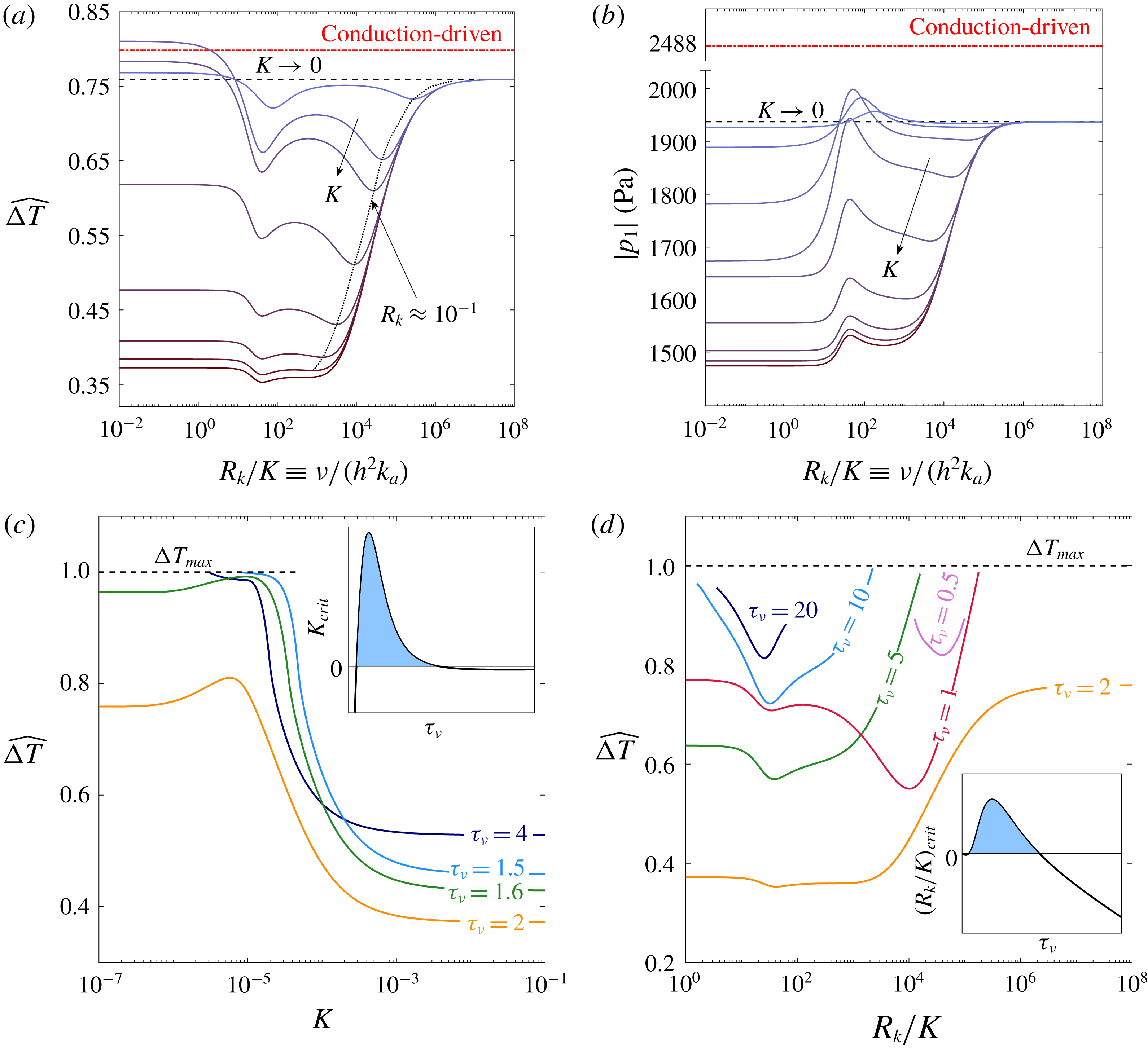
Figure 9. (a) Scaled temperature difference across the stack,
 $\widehat{\unicode[STIX]{x0394}T}=\unicode[STIX]{x0394}T/(T_{max}-T_{c})$
, and (b) maximum pressure amplitude,
$\widehat{\unicode[STIX]{x0394}T}=\unicode[STIX]{x0394}T/(T_{max}-T_{c})$
, and (b) maximum pressure amplitude,
 $|p_{1}|$
, as a function of the non-dimensional group
$|p_{1}|$
, as a function of the non-dimensional group
 $R_{k}/K$
for different values of the partition coefficient
$R_{k}/K$
for different values of the partition coefficient
 $K$
, at
$K$
, at
 $\unicode[STIX]{x1D70F}_{\unicode[STIX]{x1D708}}=2$
. (c) Value of
$\unicode[STIX]{x1D70F}_{\unicode[STIX]{x1D708}}=2$
. (c) Value of
 $\widehat{\unicode[STIX]{x0394}T}$
for the limit of fast kinetics (
$\widehat{\unicode[STIX]{x0394}T}$
for the limit of fast kinetics (
 $R_{k}\rightarrow 0$
) as a function of
$R_{k}\rightarrow 0$
) as a function of
 $K$
for different
$K$
for different
 $\unicode[STIX]{x1D70F}_{\unicode[STIX]{x1D708}}$
values. The inset presents an analytic approximation for the critical partition coefficient,
$\unicode[STIX]{x1D70F}_{\unicode[STIX]{x1D708}}$
values. The inset presents an analytic approximation for the critical partition coefficient,
 $K_{crit}$
, for which a maximum appears, as a function of
$K_{crit}$
, for which a maximum appears, as a function of
 $\unicode[STIX]{x1D70F}_{\unicode[STIX]{x1D708}}$
. (d) Value of
$\unicode[STIX]{x1D70F}_{\unicode[STIX]{x1D708}}$
. (d) Value of
 $\widehat{\unicode[STIX]{x0394}T}$
for the limit of ideal sorption (
$\widehat{\unicode[STIX]{x0394}T}$
for the limit of ideal sorption (
 $K\rightarrow \infty$
) as a function of
$K\rightarrow \infty$
) as a function of
 $R_{k}/K$
for different
$R_{k}/K$
for different
 $\unicode[STIX]{x1D70F}_{\unicode[STIX]{x1D708}}$
values. The inset presents an analytic approximation for the critical value
$\unicode[STIX]{x1D70F}_{\unicode[STIX]{x1D708}}$
values. The inset presents an analytic approximation for the critical value
 $(R_{k}/K)_{crit}$
for which a minimum appears, as a function of
$(R_{k}/K)_{crit}$
for which a minimum appears, as a function of
 $\unicode[STIX]{x1D70F}_{\unicode[STIX]{x1D708}}$
. The mean pressure is
$\unicode[STIX]{x1D70F}_{\unicode[STIX]{x1D708}}$
. The mean pressure is
 $p_{m}=1$
bar, the cold-side temperature is
$p_{m}=1$
bar, the cold-side temperature is
 $T_{c}=20\,^{\circ }\text{C}$
, the scaled stack length and location are
$T_{c}=20\,^{\circ }\text{C}$
, the scaled stack length and location are
 $L_{s}/L=0.02$
and
$L_{s}/L=0.02$
and
 $L_{0}/L=0.83$
, respectively, and the heat flux input is
$L_{0}/L=0.83$
, respectively, and the heat flux input is
 $Q_{h}=25~\text{kW}~\text{m}^{-2}$
.
$Q_{h}=25~\text{kW}~\text{m}^{-2}$
.
4.2.5 Sorption kinetics
In order to study the effects of reaction kinetics on the system’s limit cycle, we relax the assumption of ideal sorption (
 $\unicode[STIX]{x1D702}_{\unicode[STIX]{x1D708}},\unicode[STIX]{x1D702}_{D}\neq 1$
) and calculate key elements that characterise the limit cycle –
$\unicode[STIX]{x1D702}_{\unicode[STIX]{x1D708}},\unicode[STIX]{x1D702}_{D}\neq 1$
) and calculate key elements that characterise the limit cycle –
 $\unicode[STIX]{x0394}T$
and
$\unicode[STIX]{x0394}T$
and
 $|p_{1}|$
, as affected by the sorption characteristics. Figure 9(a) presents the scaled temperature difference across the stack,
$|p_{1}|$
, as affected by the sorption characteristics. Figure 9(a) presents the scaled temperature difference across the stack,
 $\widehat{\unicode[STIX]{x0394}T}$
, as a function of
$\widehat{\unicode[STIX]{x0394}T}$
, as a function of
 $R_{k}/K\equiv \unicode[STIX]{x1D708}/(h^{2}k_{a})$
, the ratio of the viscous time scale and the (forward) sorption reaction, for various values of
$R_{k}/K\equiv \unicode[STIX]{x1D708}/(h^{2}k_{a})$
, the ratio of the viscous time scale and the (forward) sorption reaction, for various values of
 $K$
. Although drawn against
$K$
. Although drawn against
 $R_{k}/K$
(instead of simply against
$R_{k}/K$
(instead of simply against
 $R_{k}$
), the curves resemble their respective curves from the stability analysis (figure 4): the left end of the curves represents the limit of fast kinetics, in which each curve flattens towards a unique
$R_{k}$
), the curves resemble their respective curves from the stability analysis (figure 4): the left end of the curves represents the limit of fast kinetics, in which each curve flattens towards a unique
 $\widehat{\unicode[STIX]{x0394}T}$
value, determined by the value of
$\widehat{\unicode[STIX]{x0394}T}$
value, determined by the value of
 $K$
– the boundary’s sorptive affinity for a given gas component. The right end of the curves represents the limit of slow kinetics, a limit to which all curves approach. However, unlike figure 4, at the system limit cycle
$K$
– the boundary’s sorptive affinity for a given gas component. The right end of the curves represents the limit of slow kinetics, a limit to which all curves approach. However, unlike figure 4, at the system limit cycle
 $K\rightarrow 0$
does not recover the known, conduction-driven thermoacoustics solution (dashed-dotted, red). The oscillatory flow, produced solely by the conduction-driven mechanism in this limit, in the presence of a temperature gradient, results in a hydrodynamic dispersion of heat down the gradient. Since
$K\rightarrow 0$
does not recover the known, conduction-driven thermoacoustics solution (dashed-dotted, red). The oscillatory flow, produced solely by the conduction-driven mechanism in this limit, in the presence of a temperature gradient, results in a hydrodynamic dispersion of heat down the gradient. Since
 $\text{d}C_{m}/\text{d}x\propto \text{d}T_{m}/\text{d}x$
, a concentration gradient is also imposed on the stack, giving rise to molecular diffusion as well as dispersion of mass down the concentration gradient. This undesired mass transfer requires more heating power to evaporate/desorb more of the reactive component, such that
$\text{d}C_{m}/\text{d}x\propto \text{d}T_{m}/\text{d}x$
, a concentration gradient is also imposed on the stack, giving rise to molecular diffusion as well as dispersion of mass down the concentration gradient. This undesired mass transfer requires more heating power to evaporate/desorb more of the reactive component, such that
 $\text{d}T_{m}/\text{d}x$
decreases, and eventually
$\text{d}T_{m}/\text{d}x$
decreases, and eventually
 $\unicode[STIX]{x0394}T_{(K\rightarrow 0)}<\unicode[STIX]{x0394}T_{(\mathit{conduction-driven})}$
.
$\unicode[STIX]{x0394}T_{(K\rightarrow 0)}<\unicode[STIX]{x0394}T_{(\mathit{conduction-driven})}$
.
As in all phase-exchange results,
 $\widehat{\unicode[STIX]{x0394}T}\leqslant 1$
is bounded by the reactive fluid depletion temperature,
$\widehat{\unicode[STIX]{x0394}T}\leqslant 1$
is bounded by the reactive fluid depletion temperature,
 $T_{max}$
(see § 4.1.1). Additionally, the stability analysis showed that all curves are further bounded by the limit
$T_{max}$
(see § 4.1.1). Additionally, the stability analysis showed that all curves are further bounded by the limit
 $K\rightarrow 0$
, recovering the conduction-driven result. Here
$K\rightarrow 0$
, recovering the conduction-driven result. Here
 $K\rightarrow 0$
does not recover the conduction-driven result, and, surprisingly, the curves are not physically bounded by the
$K\rightarrow 0$
does not recover the conduction-driven result, and, surprisingly, the curves are not physically bounded by the
 $K\rightarrow 0$
nor by the conduction-driven lines. Curves of small, finite
$K\rightarrow 0$
nor by the conduction-driven lines. Curves of small, finite
 $K$
values occasionally exceed these lines for sufficiently fast kinetics (
$K$
values occasionally exceed these lines for sufficiently fast kinetics (
 $R_{k}/K\lesssim 10$
). In order to closely examine this phenomenon, we consider the limit of fast kinetics (
$R_{k}/K\lesssim 10$
). In order to closely examine this phenomenon, we consider the limit of fast kinetics (
 $R_{k}\rightarrow 0$
), neutralising the effect of reaction kinetics and focus attention to the effect of
$R_{k}\rightarrow 0$
), neutralising the effect of reaction kinetics and focus attention to the effect of
 $K$
and
$K$
and
 $\unicode[STIX]{x1D70F}_{\unicode[STIX]{x1D708}}$
on
$\unicode[STIX]{x1D70F}_{\unicode[STIX]{x1D708}}$
on
 $\widehat{\unicode[STIX]{x0394}T}$
. We calculate
$\widehat{\unicode[STIX]{x0394}T}$
. We calculate
 $\widehat{\unicode[STIX]{x0394}T}$
as a function of
$\widehat{\unicode[STIX]{x0394}T}$
as a function of
 $K$
, and plot different curves in figure 9(c), each representing a unique
$K$
, and plot different curves in figure 9(c), each representing a unique
 $\unicode[STIX]{x1D70F}_{\unicode[STIX]{x1D708}}$
value. The
$\unicode[STIX]{x1D70F}_{\unicode[STIX]{x1D708}}$
value. The
 $\unicode[STIX]{x1D70F}_{\unicode[STIX]{x1D708}}=2$
curve matches the
$\unicode[STIX]{x1D70F}_{\unicode[STIX]{x1D708}}=2$
curve matches the
 $R_{k}/K\rightarrow 0$
limit results in figure 9(a). All the curves in figure 9(c) approach a constant value as
$R_{k}/K\rightarrow 0$
limit results in figure 9(a). All the curves in figure 9(c) approach a constant value as
 $K\rightarrow \infty$
(i.e. ideal sorption), determined by the value of
$K\rightarrow \infty$
(i.e. ideal sorption), determined by the value of
 $\unicode[STIX]{x1D70F}_{\unicode[STIX]{x1D708}}$
. Interestingly, some curves display a maximum point while others are cut off as the curve approach
$\unicode[STIX]{x1D70F}_{\unicode[STIX]{x1D708}}$
. Interestingly, some curves display a maximum point while others are cut off as the curve approach
 $\widehat{\unicode[STIX]{x0394}T}=1$
. Theoretically, all curves exhibit a maximum point, although for certain
$\widehat{\unicode[STIX]{x0394}T}=1$
. Theoretically, all curves exhibit a maximum point, although for certain
 $\unicode[STIX]{x1D70F}_{\unicode[STIX]{x1D708}}$
this point may be obtained at
$\unicode[STIX]{x1D70F}_{\unicode[STIX]{x1D708}}$
this point may be obtained at
 $\widehat{\unicode[STIX]{x0394}T}>1$
or
$\widehat{\unicode[STIX]{x0394}T}>1$
or
 $K<0$
, both representing non-physical cases. These
$K<0$
, both representing non-physical cases. These
 $\unicode[STIX]{x1D70F}_{\unicode[STIX]{x1D708}}$
, either too small or too large, yield a relatively large
$\unicode[STIX]{x1D70F}_{\unicode[STIX]{x1D708}}$
, either too small or too large, yield a relatively large
 $\widehat{\unicode[STIX]{x0394}T}$
even when
$\widehat{\unicode[STIX]{x0394}T}$
even when
 $K\rightarrow \infty$
(see figure 6
a, where
$K\rightarrow \infty$
(see figure 6
a, where
 $\unicode[STIX]{x1D702}_{\unicode[STIX]{x1D708}}=\unicode[STIX]{x1D702}_{D}=1$
is assumed), and as the boundary’s affinity for sorption is decreased, the short distance to the
$\unicode[STIX]{x1D702}_{\unicode[STIX]{x1D708}}=\unicode[STIX]{x1D702}_{D}=1$
is assumed), and as the boundary’s affinity for sorption is decreased, the short distance to the
 $\widehat{\unicode[STIX]{x0394}T}=1$
line is insufficient for a maximum to appear. This result is confirmed by an analytic approximation detailed in appendix B. The results of this approximation, presented in the inset of figure 9(c), show the qualitative trend of
$\widehat{\unicode[STIX]{x0394}T}=1$
line is insufficient for a maximum to appear. This result is confirmed by an analytic approximation detailed in appendix B. The results of this approximation, presented in the inset of figure 9(c), show the qualitative trend of
 $K_{crit}$
, the
$K_{crit}$
, the
 $K$
value leading to a maximum in the curves of figure 9(c), as a function of
$K$
value leading to a maximum in the curves of figure 9(c), as a function of
 $\unicode[STIX]{x1D70F}_{\unicode[STIX]{x1D708}}$
for
$\unicode[STIX]{x1D70F}_{\unicode[STIX]{x1D708}}$
for
 $Sc=0.6$
. As clearly seen, a positive (physical) value of
$Sc=0.6$
. As clearly seen, a positive (physical) value of
 $K_{crit}$
(shaded) is obtained only for a finite, intermediate range of
$K_{crit}$
(shaded) is obtained only for a finite, intermediate range of
 $\unicode[STIX]{x1D70F}_{\unicode[STIX]{x1D708}}$
. This result is reproduced for any
$\unicode[STIX]{x1D70F}_{\unicode[STIX]{x1D708}}$
. This result is reproduced for any
 $Sc>0$
.
$Sc>0$
.
The curves in figure 9(a) generally display two minima: the first appears at
 $R_{k}/K\approx 50$
in all curves, and the second appears at
$R_{k}/K\approx 50$
in all curves, and the second appears at
 $R_{k}\approx 10^{-1}$
, marked by a dotted line connecting the points. While the two minima are suppressed in the limit of
$R_{k}\approx 10^{-1}$
, marked by a dotted line connecting the points. While the two minima are suppressed in the limit of
 $K\rightarrow 0$
, only the second minimum is flattened for
$K\rightarrow 0$
, only the second minimum is flattened for
 $K\rightarrow \infty$
. For
$K\rightarrow \infty$
. For
 $K\rightarrow 0$
,
$K\rightarrow 0$
,
 $\unicode[STIX]{x1D702}_{n}\rightarrow \infty$
and
$\unicode[STIX]{x1D702}_{n}\rightarrow \infty$
and
 $\unicode[STIX]{x1D702}_{\unicode[STIX]{x1D708}}/\unicode[STIX]{x1D702}_{D}\rightarrow (1-F_{\unicode[STIX]{x1D708}})/(1-F_{D})$
are recovered, regardless of the value of
$\unicode[STIX]{x1D702}_{\unicode[STIX]{x1D708}}/\unicode[STIX]{x1D702}_{D}\rightarrow (1-F_{\unicode[STIX]{x1D708}})/(1-F_{D})$
are recovered, regardless of the value of
 $R_{k}$
. This limit truly suppresses the effect of reaction kinetics since the material now has no sorption affinity, and the minima vanish. If
$R_{k}$
. This limit truly suppresses the effect of reaction kinetics since the material now has no sorption affinity, and the minima vanish. If
 $K$
is small but finite, the value of
$K$
is small but finite, the value of
 $R_{k}$
dramatically affects
$R_{k}$
dramatically affects
 $\widehat{\unicode[STIX]{x0394}T}$
; the second minimum (
$\widehat{\unicode[STIX]{x0394}T}$
; the second minimum (
 $R_{k}\approx 10^{-1}$
) appears also in the stability analysis calculations (figure 4), and is a result of the boundary’s limited sorption capacity, that may be compensated by a regulated delay in desorption rate (see detailed explanation in § 4.1.3). When
$R_{k}\approx 10^{-1}$
) appears also in the stability analysis calculations (figure 4), and is a result of the boundary’s limited sorption capacity, that may be compensated by a regulated delay in desorption rate (see detailed explanation in § 4.1.3). When
 $K>10^{-1}$
, this minima disappears, leaving a short flat region before increasing towards the limit of
$K>10^{-1}$
, this minima disappears, leaving a short flat region before increasing towards the limit of
 $K\rightarrow 0$
. The first minimum (
$K\rightarrow 0$
. The first minimum (
 $R_{k}/K\approx 50$
), absent in the stability analysis calculations, remains for all
$R_{k}/K\approx 50$
), absent in the stability analysis calculations, remains for all
 $K$
. Investigating the nature of this minimum, we calculate additional curves of
$K$
. Investigating the nature of this minimum, we calculate additional curves of
 $\widehat{\unicode[STIX]{x0394}T}$
versus
$\widehat{\unicode[STIX]{x0394}T}$
versus
 $R_{k}/K$
for the limit of ideal sorption (
$R_{k}/K$
for the limit of ideal sorption (
 $K\rightarrow \infty$
) at various
$K\rightarrow \infty$
) at various
 $\unicode[STIX]{x1D70F}_{\unicode[STIX]{x1D708}}$
values. All these curves, presented in figure 9(d), show at least one minimum. For
$\unicode[STIX]{x1D70F}_{\unicode[STIX]{x1D708}}$
values. All these curves, presented in figure 9(d), show at least one minimum. For
 $\unicode[STIX]{x1D70F}_{\unicode[STIX]{x1D708}}>2$
, the minimum shifts towards small
$\unicode[STIX]{x1D70F}_{\unicode[STIX]{x1D708}}>2$
, the minimum shifts towards small
 $R_{k}/K$
. Here the boundary has a high affinity for sorption, and the value of
$R_{k}/K$
. Here the boundary has a high affinity for sorption, and the value of
 $\unicode[STIX]{x1D70F}_{\unicode[STIX]{x1D708}}$
sets the oscillation rate, for which an optimum of the reaction kinetics exists, such that
$\unicode[STIX]{x1D70F}_{\unicode[STIX]{x1D708}}$
sets the oscillation rate, for which an optimum of the reaction kinetics exists, such that
 $\widehat{\unicode[STIX]{x0394}T}$
is minimised. As
$\widehat{\unicode[STIX]{x0394}T}$
is minimised. As
 $\unicode[STIX]{x1D70F}_{\unicode[STIX]{x1D708}}$
is increased, the optimum is obtained for faster kinetics, or smaller
$\unicode[STIX]{x1D70F}_{\unicode[STIX]{x1D708}}$
is increased, the optimum is obtained for faster kinetics, or smaller
 $R_{k}/K$
values. Theoretically, there exists a critical value
$R_{k}/K$
values. Theoretically, there exists a critical value
 $(\unicode[STIX]{x1D70F}_{\unicode[STIX]{x1D708}})_{crit}$
, for which
$(\unicode[STIX]{x1D70F}_{\unicode[STIX]{x1D708}})_{crit}$
, for which
 $R_{k}/K=0$
; if
$R_{k}/K=0$
; if
 $\unicode[STIX]{x1D70F}_{\unicode[STIX]{x1D708}}>(\unicode[STIX]{x1D70F}_{\unicode[STIX]{x1D708}})_{crit}$
, the minimum point lies at
$\unicode[STIX]{x1D70F}_{\unicode[STIX]{x1D708}}>(\unicode[STIX]{x1D70F}_{\unicode[STIX]{x1D708}})_{crit}$
, the minimum point lies at
 $R_{k}/K<0$
– a non-physical result. Practically, since
$R_{k}/K<0$
– a non-physical result. Practically, since
 $\widehat{\unicode[STIX]{x0394}T}\leqslant 1$
sets a physical constraint,
$\widehat{\unicode[STIX]{x0394}T}\leqslant 1$
sets a physical constraint,
 $\unicode[STIX]{x1D70F}_{\unicode[STIX]{x1D708}}>(\unicode[STIX]{x1D70F}_{\unicode[STIX]{x1D708}})_{crit}$
curves do not yield any valid limit cycle results, and therefore curves showing no minimum cannot be drawn. For
$\unicode[STIX]{x1D70F}_{\unicode[STIX]{x1D708}}>(\unicode[STIX]{x1D70F}_{\unicode[STIX]{x1D708}})_{crit}$
curves do not yield any valid limit cycle results, and therefore curves showing no minimum cannot be drawn. For
 $\unicode[STIX]{x1D70F}_{\unicode[STIX]{x1D708}}<2$
, the second minimum point, suppressed for
$\unicode[STIX]{x1D70F}_{\unicode[STIX]{x1D708}}<2$
, the second minimum point, suppressed for
 $K\rightarrow \infty$
at
$K\rightarrow \infty$
at
 $\unicode[STIX]{x1D70F}_{\unicode[STIX]{x1D708}}\geqslant 2$
, reappears and as
$\unicode[STIX]{x1D70F}_{\unicode[STIX]{x1D708}}\geqslant 2$
, reappears and as
 $\unicode[STIX]{x1D70F}_{\unicode[STIX]{x1D708}}$
is further decreased the first minimum vanishes, leaving a single minimum that shifts towards large
$\unicode[STIX]{x1D70F}_{\unicode[STIX]{x1D708}}$
is further decreased the first minimum vanishes, leaving a single minimum that shifts towards large
 $R_{k}/K$
. If
$R_{k}/K$
. If
 $\unicode[STIX]{x1D70F}_{\unicode[STIX]{x1D708}}$
is dramatically decreased, the minimum is pushed towards very large values of
$\unicode[STIX]{x1D70F}_{\unicode[STIX]{x1D708}}$
is dramatically decreased, the minimum is pushed towards very large values of
 $R_{k}/K$
, in which the curves approach the
$R_{k}/K$
, in which the curves approach the
 $K\rightarrow 0$
limit, where the minimum is, again, suppressed. As before, the
$K\rightarrow 0$
limit, where the minimum is, again, suppressed. As before, the
 $\widehat{\unicode[STIX]{x0394}T}\leqslant 1$
constraint makes it impossible to draw such curves, as their results exceed
$\widehat{\unicode[STIX]{x0394}T}\leqslant 1$
constraint makes it impossible to draw such curves, as their results exceed
 $\widehat{\unicode[STIX]{x0394}T}=1$
well before the minimum disappears. In the absence of numerical evidence to support our claim, we seek an analytic approximation proving that a minimum is obtained for only a finite range of
$\widehat{\unicode[STIX]{x0394}T}=1$
well before the minimum disappears. In the absence of numerical evidence to support our claim, we seek an analytic approximation proving that a minimum is obtained for only a finite range of
 $\unicode[STIX]{x1D70F}_{\unicode[STIX]{x1D708}}$
. The details of this approximation appear in appendix B, and its results, presented in the inset of figure 9(d), show
$\unicode[STIX]{x1D70F}_{\unicode[STIX]{x1D708}}$
. The details of this approximation appear in appendix B, and its results, presented in the inset of figure 9(d), show
 $(R_{k}/K)_{crit}$
, namely the
$(R_{k}/K)_{crit}$
, namely the
 $R_{k}/K$
value leading to a minimum in the curves of figure 9(d), as a function of
$R_{k}/K$
value leading to a minimum in the curves of figure 9(d), as a function of
 $\unicode[STIX]{x1D70F}_{\unicode[STIX]{x1D708}}$
for
$\unicode[STIX]{x1D70F}_{\unicode[STIX]{x1D708}}$
for
 $Sc=0.6$
. These results indicate that a minimum in
$Sc=0.6$
. These results indicate that a minimum in
 $\widehat{\unicode[STIX]{x0394}T}$
should only be obtained for a finite, intermediate range of
$\widehat{\unicode[STIX]{x0394}T}$
should only be obtained for a finite, intermediate range of
 $\unicode[STIX]{x1D70F}_{\unicode[STIX]{x1D708}}$
, since
$\unicode[STIX]{x1D70F}_{\unicode[STIX]{x1D708}}$
, since
 $(R_{k}/K)_{crit}<0$
does not represent a physically valid solution.
$(R_{k}/K)_{crit}<0$
does not represent a physically valid solution.
The effect of reaction kinetics on a thermoacoustic system vary according to the system’s objective: for minimising
 $\unicode[STIX]{x0394}T$
, controlling
$\unicode[STIX]{x0394}T$
, controlling
 $R_{k}$
proves to be beneficial even if
$R_{k}$
proves to be beneficial even if
 $K\rightarrow \infty$
, but works to the contrary if one wishes to maximise
$K\rightarrow \infty$
, but works to the contrary if one wishes to maximise
 ${\dot{W}}$
, since the minimum in
${\dot{W}}$
, since the minimum in
 $\widehat{\unicode[STIX]{x0394}T}$
imposes an undesired minimum on
$\widehat{\unicode[STIX]{x0394}T}$
imposes an undesired minimum on
 $\unicode[STIX]{x1D703}\equiv ||\unicode[STIX]{x1D719}|-90^{\circ }|$
such that
$\unicode[STIX]{x1D703}\equiv ||\unicode[STIX]{x1D719}|-90^{\circ }|$
such that
 ${\dot{W}}$
is also lowered. This effect is clearly seen in figure 9(b), showing the maximum pressure amplitude,
${\dot{W}}$
is also lowered. This effect is clearly seen in figure 9(b), showing the maximum pressure amplitude,
 $|p_{1}|$
, as a function of
$|p_{1}|$
, as a function of
 $R_{k}/K$
. The nearly monotonically increasing nature of the curves, linking the limits of fast and slow kinetics, is disturbed by a local maximum point, exactly matching the minimum points at
$R_{k}/K$
. The nearly monotonically increasing nature of the curves, linking the limits of fast and slow kinetics, is disturbed by a local maximum point, exactly matching the minimum points at
 $R_{k}/K\approx 50$
in figure 9(a). The increase in
$R_{k}/K\approx 50$
in figure 9(a). The increase in
 $|p_{1}|$
cannot be attributed to the decrease in
$|p_{1}|$
cannot be attributed to the decrease in
 $\widehat{\unicode[STIX]{x0394}T}$
directly, since the latter decreases the system’s thermal potential. However, the subsequent effect of the minimum in
$\widehat{\unicode[STIX]{x0394}T}$
directly, since the latter decreases the system’s thermal potential. However, the subsequent effect of the minimum in
 $\widehat{\unicode[STIX]{x0394}T}$
on
$\widehat{\unicode[STIX]{x0394}T}$
on
 $\unicode[STIX]{x1D719}$
alters the wave form such that a nearly pure standing wave is obtained, for which
$\unicode[STIX]{x1D719}$
alters the wave form such that a nearly pure standing wave is obtained, for which
 $|p_{1}|$
increases in spite of the decrease in
$|p_{1}|$
increases in spite of the decrease in
 ${\dot{W}}$
. All values of
${\dot{W}}$
. All values of
 $|p_{1}|$
here are smaller than the conduction-driven reference values. Although
$|p_{1}|$
here are smaller than the conduction-driven reference values. Although
 $\widehat{\unicode[STIX]{x0394}T}$
may exceed the conduction-driven value for
$\widehat{\unicode[STIX]{x0394}T}$
may exceed the conduction-driven value for
 $R_{k}\rightarrow 0$
, thus maximising the system thermal potential, the wave form deviates from a standing wave appreciably, resulting in a small, minimal value of
$R_{k}\rightarrow 0$
, thus maximising the system thermal potential, the wave form deviates from a standing wave appreciably, resulting in a small, minimal value of
 $|p_{1}|$
. At the local maximum (
$|p_{1}|$
. At the local maximum (
 $R_{k}/K\approx 50$
), the resemblance of wave form to a pure standing wave increases
$R_{k}/K\approx 50$
), the resemblance of wave form to a pure standing wave increases
 $|p_{1}|$
, such that for finite
$|p_{1}|$
, such that for finite
 $K$
values the
$K$
values the
 $K\rightarrow 0$
limit is breached. The local minimum in
$K\rightarrow 0$
limit is breached. The local minimum in
 $\widehat{\unicode[STIX]{x0394}T}$
decreases the system thermal potential, such that the maximal phase-exchange pressure amplitude (
$\widehat{\unicode[STIX]{x0394}T}$
decreases the system thermal potential, such that the maximal phase-exchange pressure amplitude (
 $|p_{1}|\approx 2000~\text{Pa}$
) is considerably smaller than the conduction-driven value (
$|p_{1}|\approx 2000~\text{Pa}$
) is considerably smaller than the conduction-driven value (
 $|p_{1}|=2488~\text{Pa}$
).
$|p_{1}|=2488~\text{Pa}$
).
5 Concluding remarks
In this work, we theoretically examined a new mechanism of heat transfer in thermoacoustics, in which heat and mass are isothermally transferred between the working fluid and a sorbent boundary in the form of latent heat, rather than through conduction. Beginning with the conservation equations for a gas mixture in their most general form, we used an asymptotic expansion to de-couple the equations and simplify them into a set of ordinary differential equations. These equations were solved and manipulated into the form of a wave equation, and used to derive transport quantities, ultimately leading to the derivation of a differential equation for the axial temperature gradient imposed on the stack. The derived equations were subsequently used for a stability and limit cycle analyses. In the calculations we demonstrated how modifying a gas mixture to contain a reactive gas, able to exchange mass with a sorbent layer, decreases the temperature difference required to trigger an instability in thermoacoustic systems. These findings are in good agreement with experimental results obtained for an air–water mixture (Tsuda & Ueda Reference Tsuda and Ueda2017).
Onset temperature differences of various gas mixtures were compared, with the lowest values found for mixtures employing an inert component with a low heat capacity and reactive component with a low boiling temperature. Within our selection of gas mixtures, the air–MeOH mixture exhibited the lowest temperature difference required for onset of acoustic oscillations. Effects of gas mixture composition were investigated, revealing a clear dependency of the onset temperature difference on the reactive gas concentration
 $C_{m}$
. As only the reactive gas is able to exchange phase with the sorbent boundary, increasing its fraction in the mixture enhances the effect, and hence decreases the onset temperature difference. A non-dimensional number,
$C_{m}$
. As only the reactive gas is able to exchange phase with the sorbent boundary, increasing its fraction in the mixture enhances the effect, and hence decreases the onset temperature difference. A non-dimensional number,
 $\unicode[STIX]{x1D713}=(C_{m}/(1-C_{m}))(l_{h}/RT_{m})$
, was found to be a good indicator for evaluating the performance of different sorbent/sorbate pairs, characterised by the sorbent/gas equilibrium curve shape, the latent heat released in the process and the gas mixture temperature.
$\unicode[STIX]{x1D713}=(C_{m}/(1-C_{m}))(l_{h}/RT_{m})$
, was found to be a good indicator for evaluating the performance of different sorbent/sorbate pairs, characterised by the sorbent/gas equilibrium curve shape, the latent heat released in the process and the gas mixture temperature.
The limit cycle analysis revealed that, with the addition of boundary mass exchange increasing
 $C_{m}$
significantly alters the wave form in the system, shifting it away from a standing-wave behaviour. The mass exchange within the stack results in recurrent injection/ejection of the reactive gas to/from the gas mixture, and thus intervenes with the natural tendency of the wave to resemble a standing wave. This wave-form distortion increases the acoustic power in the system despite the decrease in pressure amplitude. Additionally, it also tends to decrease the resonant frequency as the travelling-wave component becomes dominant.
$C_{m}$
significantly alters the wave form in the system, shifting it away from a standing-wave behaviour. The mass exchange within the stack results in recurrent injection/ejection of the reactive gas to/from the gas mixture, and thus intervenes with the natural tendency of the wave to resemble a standing wave. This wave-form distortion increases the acoustic power in the system despite the decrease in pressure amplitude. Additionally, it also tends to decrease the resonant frequency as the travelling-wave component becomes dominant.
Effects of the reactive gas concentration,
 $C_{m}$
, and the Womersley number,
$C_{m}$
, and the Womersley number,
 $\unicode[STIX]{x1D70F}_{\unicode[STIX]{x1D708}}$
on a system’s limit cycle temperature difference and pressure amplitude (
$\unicode[STIX]{x1D70F}_{\unicode[STIX]{x1D708}}$
on a system’s limit cycle temperature difference and pressure amplitude (
 $\unicode[STIX]{x0394}T$
and
$\unicode[STIX]{x0394}T$
and
 $|p_{1}|$
) were examined. As expected, if
$|p_{1}|$
) were examined. As expected, if
 $C_{m}$
is increased
$C_{m}$
is increased
 $\unicode[STIX]{x0394}T$
and
$\unicode[STIX]{x0394}T$
and
 $|p_{1}|$
decrease. The dependency on
$|p_{1}|$
decrease. The dependency on
 $\unicode[STIX]{x1D70F}_{\unicode[STIX]{x1D708}}$
is far less trivial: the trend of
$\unicode[STIX]{x1D70F}_{\unicode[STIX]{x1D708}}$
is far less trivial: the trend of
 $|p_{1}|$
versus
$|p_{1}|$
versus
 $\unicode[STIX]{x1D70F}_{\unicode[STIX]{x1D708}}$
at intermediate
$\unicode[STIX]{x1D70F}_{\unicode[STIX]{x1D708}}$
at intermediate
 $\unicode[STIX]{x1D70F}_{\unicode[STIX]{x1D708}}$
values may resemble a conduction-driven system, in which
$\unicode[STIX]{x1D70F}_{\unicode[STIX]{x1D708}}$
values may resemble a conduction-driven system, in which
 $|p_{1}|$
and
$|p_{1}|$
and
 $\unicode[STIX]{x0394}T$
minimise simultaneously since the pressure amplitude is proportional to the system thermal potential. However, at small or large
$\unicode[STIX]{x0394}T$
minimise simultaneously since the pressure amplitude is proportional to the system thermal potential. However, at small or large
 $\unicode[STIX]{x1D70F}_{\unicode[STIX]{x1D708}}$
, as
$\unicode[STIX]{x1D70F}_{\unicode[STIX]{x1D708}}$
, as
 $\unicode[STIX]{x0394}T$
approaches its maximum value the wave form is greatly distorted, deviating from that of a standing wave. As a result,
$\unicode[STIX]{x0394}T$
approaches its maximum value the wave form is greatly distorted, deviating from that of a standing wave. As a result,
 $|p_{1}|$
decreases as a system is forced to operate near its limiting
$|p_{1}|$
decreases as a system is forced to operate near its limiting
 $\unicode[STIX]{x1D70F}_{\unicode[STIX]{x1D708}}$
values. At very large
$\unicode[STIX]{x1D70F}_{\unicode[STIX]{x1D708}}$
values. At very large
 $C_{m}$
, any resemblance to a conduction-driven system disappears and the phase-exchange system reveals a completely opposite trend – reaching a maximum for
$C_{m}$
, any resemblance to a conduction-driven system disappears and the phase-exchange system reveals a completely opposite trend – reaching a maximum for
 $\unicode[STIX]{x1D70F}_{\unicode[STIX]{x1D708}}\approx 2$
and decreasing for small and large
$\unicode[STIX]{x1D70F}_{\unicode[STIX]{x1D708}}\approx 2$
and decreasing for small and large
 $\unicode[STIX]{x1D70F}_{\unicode[STIX]{x1D708}}$
.
$\unicode[STIX]{x1D70F}_{\unicode[STIX]{x1D708}}$
.
Given a system sustaining a limit cycle, increasing the heat input
 $Q_{h}$
results in increased
$Q_{h}$
results in increased
 $|p_{1}|$
while
$|p_{1}|$
while
 $\unicode[STIX]{x0394}T$
remains constant. This non-intuitive result is explained by a simple analytic approximation, demonstrating how the proportionality
$\unicode[STIX]{x0394}T$
remains constant. This non-intuitive result is explained by a simple analytic approximation, demonstrating how the proportionality
 $Q_{h}\propto |p_{1}|^{2}$
, characterising standing-wave systems, yields a nearly constant temperature gradient in the stack.
$Q_{h}\propto |p_{1}|^{2}$
, characterising standing-wave systems, yields a nearly constant temperature gradient in the stack.
Finally, we examined the effects of reaction kinetics on system stability as well as its limit cycle characteristics. The stability limit was calculated for various values of
 $K$
, representing different sorbent affinities for the reactive component. Above a certain value of
$K$
, representing different sorbent affinities for the reactive component. Above a certain value of
 $K$
, sorption kinetics result in monotonically increasing stability curves, displaying the lowest and highest temperature differences in the limit of fast and slow kinetics, respectively. A curious result is obtained for low values of
$K$
, sorption kinetics result in monotonically increasing stability curves, displaying the lowest and highest temperature differences in the limit of fast and slow kinetics, respectively. A curious result is obtained for low values of
 $K$
, in which the optimum for
$K$
, in which the optimum for
 $\unicode[STIX]{x0394}T_{onset}$
is not in the limit of fast kinetics. Allowing partial relaxation for the desorbing gas in these cases proves to be beneficial, since the boundary affinity for sorption is highly limited. As opposed to the stability analysis, the limit of slow kinetics for a system limit cycle does not recover the conduction-driven result. Hydrodynamic dispersion of mass exists down the concentration gradient even if the oscillatory flow is induced by the conduction-driven mechanism. Moreover, a non-trivial minimum for
$\unicode[STIX]{x0394}T_{onset}$
is not in the limit of fast kinetics. Allowing partial relaxation for the desorbing gas in these cases proves to be beneficial, since the boundary affinity for sorption is highly limited. As opposed to the stability analysis, the limit of slow kinetics for a system limit cycle does not recover the conduction-driven result. Hydrodynamic dispersion of mass exists down the concentration gradient even if the oscillatory flow is induced by the conduction-driven mechanism. Moreover, a non-trivial minimum for
 $\unicode[STIX]{x0394}T$
is obtained even if ideal sorption is assumed (
$\unicode[STIX]{x0394}T$
is obtained even if ideal sorption is assumed (
 $K\rightarrow \infty$
). A finite value of the dimensionless group
$K\rightarrow \infty$
). A finite value of the dimensionless group
 $R_{k}/K\equiv \unicode[STIX]{x1D708}/(h^{2}k_{a})$
is found to minimise
$R_{k}/K\equiv \unicode[STIX]{x1D708}/(h^{2}k_{a})$
is found to minimise
 $\unicode[STIX]{x0394}T$
for practically any
$\unicode[STIX]{x0394}T$
for practically any
 $K$
and
$K$
and
 $\unicode[STIX]{x1D70F}_{\unicode[STIX]{x1D708}}$
.
$\unicode[STIX]{x1D70F}_{\unicode[STIX]{x1D708}}$
.
The results laid out in this work provide incentive for the use of phase-exchange thermoacoustics in the design of heat engines, capable of operating at low temperature differences and possibly produce higher acoustic power. As most low-grade heat sources are not sufficient for operation of commercially available heat engines, as well as conduction-driven thermoacoustic devices, phase-exchange thermoacoustic heat engines provide a promising alternative for exploiting these abundant heat sources.
Acknowledgements
The research was partially supported by grant 216-11-024 from the Israel Ministry of Energy and Water, and grant no. 345/13 from the Israel Science Foundation. The authors acknowledge the support from the Nancy and Stephen Grand Technion Energy Program (GTEP).
Appendix A.
In what follows we show that the non-dimensional parameter
 $\unicode[STIX]{x1D713}$
is a monotonically decreasing function of the mean pressure. We begin by rewriting the definition
$\unicode[STIX]{x1D713}$
is a monotonically decreasing function of the mean pressure. We begin by rewriting the definition
 $$\begin{eqnarray}\unicode[STIX]{x1D713}=\frac{C_{m}}{1-C_{m}}\frac{l_{h}}{RT_{m}},\end{eqnarray}$$
noting
 $\unicode[STIX]{x1D713}=f(C_{m},l_{h},T_{m})$
. Next, we expand
$\unicode[STIX]{x1D713}=f(C_{m},l_{h},T_{m})$
. Next, we expand
 $\text{d}\unicode[STIX]{x1D713}/\text{d}p_{m}$
as
$\text{d}\unicode[STIX]{x1D713}/\text{d}p_{m}$
as
 $$\begin{eqnarray}\displaystyle \frac{\text{d}\unicode[STIX]{x1D713}}{\text{d}p_{m}} & = & \displaystyle \left(\frac{\unicode[STIX]{x2202}\unicode[STIX]{x1D713}}{\unicode[STIX]{x2202}C_{m}}\right)_{l_{h},T_{m}}\frac{\text{d}C_{m}}{\text{d}p_{m}}+\left(\frac{\unicode[STIX]{x2202}\unicode[STIX]{x1D713}}{\unicode[STIX]{x2202}l_{h}}\right)_{C_{m},T_{m}}\frac{\text{d}l_{h}}{\text{d}p_{m}}+\left(\frac{\unicode[STIX]{x2202}\unicode[STIX]{x1D713}}{\unicode[STIX]{x2202}T_{m}}\right)_{C_{m},l_{h}}\frac{\text{d}T_{m}}{\text{d}p_{m}}\nonumber\\ \displaystyle & = & \displaystyle \unicode[STIX]{x1D713}\left[\frac{1}{C_{m}(1-C_{m})}\frac{\text{d}C_{m}}{\text{d}p_{m}}+\frac{1}{l_{h}}\frac{\text{d}l_{h}}{\text{d}p_{m}}-\frac{1}{T_{m}}\frac{\text{d}T_{m}}{\text{d}p_{m}}\right].\end{eqnarray}$$
For simplicity, we consider the case of phase change through evaporation/condensation, in which
 $C_{m}$
and
$C_{m}$
and
 $l_{h}$
are intuitively dependent on the mean pressure
$l_{h}$
are intuitively dependent on the mean pressure
 $p_{m}$
. As
$p_{m}$
. As
 $p_{m}$
is increased towards the critical pressure, the latent heat of evaporation decreases (
$p_{m}$
is increased towards the critical pressure, the latent heat of evaporation decreases (
 $\text{d}l_{h}/\text{d}p_{m}<0$
) and the boiling temperature increases, such that
$\text{d}l_{h}/\text{d}p_{m}<0$
) and the boiling temperature increases, such that
 $\text{d}C_{m}/\text{d}p_{m}<0$
. The temperature can only increases with pressure; hence,
$\text{d}C_{m}/\text{d}p_{m}<0$
. The temperature can only increases with pressure; hence,
 $\text{d}T_{m}/\text{d}p_{m}>0$
. All the terms multiplying the derivatives in (A 2) are positive. It is, therefore, clear that all three terms on the right-hand side of (A 2) are negative, and consequently
$\text{d}T_{m}/\text{d}p_{m}>0$
. All the terms multiplying the derivatives in (A 2) are positive. It is, therefore, clear that all three terms on the right-hand side of (A 2) are negative, and consequently
 $\text{d}\unicode[STIX]{x1D713}/\text{d}p_{m}<0$
.
$\text{d}\unicode[STIX]{x1D713}/\text{d}p_{m}<0$
.
Appendix B.
Here, we describe the analytic approximation used in § 4.2.5 to show that extremum points in the temperature difference across the stack,
 $\unicode[STIX]{x0394}T$
, at a given heating power, may only be obtained for a finite range of the Womersley number,
$\unicode[STIX]{x0394}T$
, at a given heating power, may only be obtained for a finite range of the Womersley number,
 $\unicode[STIX]{x1D70F}_{\unicode[STIX]{x1D708}}$
. The total power in a system is comprised of three fundamental elements: acoustic power, hydrodynamic dispersion and diffusion. Each of these terms appears twice in (2.65) – once for the conduction-driven and once for the phase-exchange mechanisms. In order to understand the effect of sorption kinetics, we only refer to the phase-exchange terms in (2.65); the typically weak effect of molecular diffusion on
$\unicode[STIX]{x1D70F}_{\unicode[STIX]{x1D708}}$
. The total power in a system is comprised of three fundamental elements: acoustic power, hydrodynamic dispersion and diffusion. Each of these terms appears twice in (2.65) – once for the conduction-driven and once for the phase-exchange mechanisms. In order to understand the effect of sorption kinetics, we only refer to the phase-exchange terms in (2.65); the typically weak effect of molecular diffusion on
 $\unicode[STIX]{x0394}T$
is neglected for the simplicity of this approximation. If a minimum of the heat converted to acoustic power is dispersed down the concentration (and temperature) gradient,
$\unicode[STIX]{x0394}T$
is neglected for the simplicity of this approximation. If a minimum of the heat converted to acoustic power is dispersed down the concentration (and temperature) gradient,
 $\unicode[STIX]{x0394}T$
is maximised. The converse of this statement is also correct: maximising the dispersion minimises
$\unicode[STIX]{x0394}T$
is maximised. The converse of this statement is also correct: maximising the dispersion minimises
 $\unicode[STIX]{x0394}T$
. We define a new variable,
$\unicode[STIX]{x0394}T$
. We define a new variable,
 $\unicode[STIX]{x1D6F4}$
, as the sum of phase-exchange acoustic power production and the (negative) heat flux due to hydrodynamic dispersion of the reactive component,
$\unicode[STIX]{x1D6F4}$
, as the sum of phase-exchange acoustic power production and the (negative) heat flux due to hydrodynamic dispersion of the reactive component,
 $$\begin{eqnarray}\unicode[STIX]{x1D6F4}=G_{1}\text{Re}\left[\frac{\widetilde{p_{1}}u_{1}}{\unicode[STIX]{x1D702}_{D}}\left(\frac{F_{D}-\widetilde{F_{\unicode[STIX]{x1D708}}}}{\widetilde{F_{\unicode[STIX]{x1D708}}}}\right)\right]-G_{2}\text{Im}\left[\widetilde{F_{\unicode[STIX]{x1D708}}}(1+Sc)-\frac{\unicode[STIX]{x1D702}_{\unicode[STIX]{x1D708}}}{\unicode[STIX]{x1D702}_{D}}(\widetilde{F_{\unicode[STIX]{x1D708}}}-F_{D})\right],\end{eqnarray}$$
where
 $G_{1}$
and
$G_{1}$
and
 $G_{2}$
contain all the other physical variables in these two terms. The pressure and velocity may be expressed using the standing-wave approximation (§ 3.1.2) by (3.9)–(3.10), such that
$G_{2}$
contain all the other physical variables in these two terms. The pressure and velocity may be expressed using the standing-wave approximation (§ 3.1.2) by (3.9)–(3.10), such that
 $\widetilde{p_{1}}u_{1}\approx \text{i}p_{A}^{2}\sin (2x)/2$
. For the sake of simplicity, as they serve merely as numerical pre-factors, we set
$\widetilde{p_{1}}u_{1}\approx \text{i}p_{A}^{2}\sin (2x)/2$
. For the sake of simplicity, as they serve merely as numerical pre-factors, we set
 $G_{1}p_{A}^{2}\sin (2x)/2=G_{2}=1$
, to obtain
$G_{1}p_{A}^{2}\sin (2x)/2=G_{2}=1$
, to obtain
 $$\begin{eqnarray}\unicode[STIX]{x1D6F4}\approx -\left\{\text{Im}\left[\frac{F_{D}-\widetilde{F_{\unicode[STIX]{x1D708}}}}{\unicode[STIX]{x1D702}_{D}\widetilde{F_{\unicode[STIX]{x1D708}}}}\right]+\text{Im}\left[\widetilde{F_{\unicode[STIX]{x1D708}}}(1+Sc)-\frac{\unicode[STIX]{x1D702}_{\unicode[STIX]{x1D708}}}{\unicode[STIX]{x1D702}_{D}}(\widetilde{F_{\unicode[STIX]{x1D708}}}-F_{D})\right]\right\}.\end{eqnarray}$$
We simplify the kinetics parameter, given explicitly in (2.47), by keeping only its dependence on
 $K$
and
$K$
and
 $R_{k}$
such that
$R_{k}$
such that
 $$\begin{eqnarray}\unicode[STIX]{x1D702}_{n}\approx 1+\frac{1-F_{n}}{K}+\text{i}\frac{R_{k}}{K}(1-F_{n}).\end{eqnarray}$$
Further simplifying
 $\unicode[STIX]{x1D6F4}$
, we consider the high frequency limit (also termed the ‘boundary layer approximation’ by Swift Reference Swift1988), such that
$\unicode[STIX]{x1D6F4}$
, we consider the high frequency limit (also termed the ‘boundary layer approximation’ by Swift Reference Swift1988), such that
 $F_{\unicode[STIX]{x1D708}}=1-\hat{\unicode[STIX]{x1D70F}}_{\unicode[STIX]{x1D708}}^{-1}$
and
$F_{\unicode[STIX]{x1D708}}=1-\hat{\unicode[STIX]{x1D70F}}_{\unicode[STIX]{x1D708}}^{-1}$
and
 $F_{D}=1-\hat{\unicode[STIX]{x1D70F}}_{\unicode[STIX]{x1D708}}^{-1}Sc^{-1/2}$
.
$F_{D}=1-\hat{\unicode[STIX]{x1D70F}}_{\unicode[STIX]{x1D708}}^{-1}Sc^{-1/2}$
.
For the approximation presented in figure 9(c) we set
 $R_{k}\rightarrow 0$
, such that
$R_{k}\rightarrow 0$
, such that
 $\unicode[STIX]{x1D702}_{n}\approx 1+(1-F_{n})/K$
. Setting
$\unicode[STIX]{x1D702}_{n}\approx 1+(1-F_{n})/K$
. Setting
 $\text{d}\unicode[STIX]{x1D6F4}/\text{d}K=0$
yields a quadratic equation for
$\text{d}\unicode[STIX]{x1D6F4}/\text{d}K=0$
yields a quadratic equation for
 $K$
, to which
$K$
, to which
 $K_{crit}=f(\unicode[STIX]{x1D70F}_{\unicode[STIX]{x1D708}},Sc)$
, namely the critical partition coefficient for which a maximum in
$K_{crit}=f(\unicode[STIX]{x1D70F}_{\unicode[STIX]{x1D708}},Sc)$
, namely the critical partition coefficient for which a maximum in
 $\unicode[STIX]{x0394}T$
is obtained, is the solution. In one of the two solutions satisfying the equation,
$\unicode[STIX]{x0394}T$
is obtained, is the solution. In one of the two solutions satisfying the equation,
 $K_{crit}<0$
is obtained for all
$K_{crit}<0$
is obtained for all
 $\unicode[STIX]{x1D70F}_{\unicode[STIX]{x1D708}}$
and
$\unicode[STIX]{x1D70F}_{\unicode[STIX]{x1D708}}$
and
 $Sc$
. In the second solution, however, positive values of
$Sc$
. In the second solution, however, positive values of
 $K_{crit}$
are obtained for a finite, intermediate range of
$K_{crit}$
are obtained for a finite, intermediate range of
 $\unicode[STIX]{x1D70F}_{\unicode[STIX]{x1D708}}$
regardless of the value assigned to
$\unicode[STIX]{x1D70F}_{\unicode[STIX]{x1D708}}$
regardless of the value assigned to
 $Sc$
. This qualitative behaviour is sketched in the inset of figure 9(c) for
$Sc$
. This qualitative behaviour is sketched in the inset of figure 9(c) for
 $Sc=0.6$
, a representative value for an air–water vapour gas mixture.
$Sc=0.6$
, a representative value for an air–water vapour gas mixture.
The approximation presented in figure 9(d) is nearly identical to that of figure 9(c). Here we set
 $K\rightarrow \infty$
, such that
$K\rightarrow \infty$
, such that
 $\unicode[STIX]{x1D702}_{n}\approx 1+\text{i}(R_{k}/K)(1-F_{n})$
, and derive a quadratic equation for
$\unicode[STIX]{x1D702}_{n}\approx 1+\text{i}(R_{k}/K)(1-F_{n})$
, and derive a quadratic equation for
 $R_{k}/K$
by seeking the solution of
$R_{k}/K$
by seeking the solution of
 $\text{d}\unicode[STIX]{x1D6F4}/\text{d}(R_{k}/K)=0$
. Again, only one of the solutions yields a physical result of
$\text{d}\unicode[STIX]{x1D6F4}/\text{d}(R_{k}/K)=0$
. Again, only one of the solutions yields a physical result of
 $(R_{k}/K)_{crit}>0$
for a finite range of
$(R_{k}/K)_{crit}>0$
for a finite range of
 $\unicode[STIX]{x1D70F}_{\unicode[STIX]{x1D708}}$
and any positive
$\unicode[STIX]{x1D70F}_{\unicode[STIX]{x1D708}}$
and any positive
 $Sc$
. A plot of
$Sc$
. A plot of
 $(R_{k}/K)_{crit}$
versus
$(R_{k}/K)_{crit}$
versus
 $\unicode[STIX]{x1D70F}_{\unicode[STIX]{x1D708}}$
for
$\unicode[STIX]{x1D70F}_{\unicode[STIX]{x1D708}}$
for
 $Sc=0.6$
is sketched in the inset of figure 9(d).
$Sc=0.6$
is sketched in the inset of figure 9(d).