2.1. Numerical experiments

The parameters of the DNSs used for our analysis are summarized in table 1, and are described in more detail by Lozano-Durán & Jiménez (Reference Lozano-Durán and Jiménez2014). Briefly, the code is similar to that of Kim, Moin & Moser (Reference Kim, Moin and Moser1987). The numerical discretization is dealiased Fourier in the two wall-parallel directions, and either Chebychev or seven-point compact finite differences in the wall-normal one. Throughout this paper, $u$ , $v$ and $w$ are streamwise, wall-normal and spanwise velocity fluctuations, measured with respect to their mean, which is defined over the two homogeneous directions and time. The streamwise and spanwise coordinates are $x$ and $z$ , and the wall-normal coordinate, $y$ , is zero at the wall. The only non-zero mean velocity is $U(y)$ and primed ( ${\it\phi}^{\prime }$ ) variables denote root-mean-squared (r.m.s.) intensities. The channel half-height is $h$ , and ‘ $+$ ’ superscripts denote wall units defined in terms of the friction velocity $u_{{\it\tau}}$ and of the kinematic viscosity ${\it\nu}$ . The Kármán number is $\mathit{Re}_{{\it\tau}}=u_{{\it\tau}}h/{\it\nu}$ . We define the global eddy-turnover time as $h/u_{{\it\tau}}$ , and occasionally use a local turnover time  $y/u_{{\it\tau}}$ . The Kolmogorov length and time scales are ${\it\eta}=({\it\nu}^{3}/{\it\varepsilon})^{1/4}$ and $t_{{\it\eta}}=({\it\nu}/{\it\varepsilon})^{1/2}$ , respectively, where ${\it\varepsilon}(y)$ is the mean dissipation rate of the kinetic energy. We often classify results in terms of buffer, logarithmic and outer regions, arbitrarily defined as $y^{+}<100$ , $100{\it\nu}/u_{{\it\tau}}<y<0.2h$ and $y>0.2h$ , respectively. It was checked that varying those limits within the usual range did not significantly alter the results presented below.

The Reynolds numbers chosen, $\mathit{Re}_{{\it\tau}}=932$ , 2009 and 4164, yield scale separations of $h/10{\it\eta}\simeq 30$ , 60 and 100, respectively, if we assume that the largest structures are $O(h)$ and that the smallest ones are vortices with diameters of order $10{\it\eta}$ (Jiménez et al. Reference Jiménez, Wray, Saffman and Rogallo1993; Jiménez & Wray Reference Jiménez and Wray1998). The microscale Reynolds numbers in table 1 are computed, assuming isotropy, as $\mathit{Re}_{{\it\lambda}}=q^{2}\sqrt{5/(3{\it\nu}{\it\varepsilon})}$ , where $q^{2}=u^{2}+v^{2}+w^{2}$ , and the maximum is achieved in all cases near $y/h=0.4$ . All of the statistics are compiled over at least 10 global eddy turnovers, which will be seen in § 5.1 to be long enough with respect to the lifetimes of most coherent structures not to interference with their description.

The analysis of the temporal evolution of the flow requires storing approximately $10^{4}$ snapshots for each simulation, implying several hundred terabytes for each channel in table 1. To keep the storage requirements under some control, the channel dimensions are kept $L_{x}=2{\rm\pi}h$ and $L_{z}={\rm\pi}h$ . It was shown by Flores & Jimenez (Reference Flores and Jiménez2010) that this box size is the minimum needed to accommodate the widest flow structures, and Lozano-Durán & Jiménez (Reference Lozano-Durán and Jiménez2014) showed that it results in correct one-point statistics. Structures longer than $2{\rm\pi}h$ exist in larger channels (Jiménez Reference Jiménez1998; Kim & Adrian Reference Kim and Adrian1999; Marusic Reference Marusic2001; del Álamo et al. Reference del Álamo, Jiménez, Zandonade and Moser2004; Jiménez, del Álamo & Flores Reference Jiménez, del Álamo and Flores2004; Guala, Hommema & Adrian Reference Guala, Hommema and Adrian2006), and are represented in the numerics as infinitely long, but it was argued by del Álamo et al. (Reference del Álamo, Jiménez, Zandonade and Moser2004) and Lozano-Durán & Jiménez (Reference Lozano-Durán and Jiménez2014) that their evolution times are slow enough for their interactions with the smaller scales to be represented correctly even in that case. The result is essentially healthy turbulence across the whole channel, although the behaviour of the largest structures is probably unreliable. However, spectral analysis shows that structures longer than $2{\rm\pi}h$ are at least as tall as $h$ (Hoyas & Jimenez Reference Hoyas and Jiménez2006; Jiménez Reference Jiménez2012), so that the results of our analysis should be correct for eddies approximately restricted to the logarithmic and buffer layers. In fact, no structure has been discarded from our analysis for being too large. The number of eddies constricted by the box size is too small to influence the statistics, and the only obvious difference between our results and those in larger boxes is the ‘cap’ of very tall and long structures found in the size distributions in figure 5 of Lozano-Durán et al. (Reference Lozano-Durán, Flores and Jiménez2012), which is much weaker in the equivalent distributions in figure 8(c,d) of the present paper.

2.2. Identification of coherent structures

In the present work, we understand by coherent structures those motions that are organized in space and persistent in time and, although some distinctions are made in the literature, we will use as synonymous coherent structures, objects and eddies.

We define structures as simply connected sets of points in which some property exceeds a given threshold, with connectivity defined in terms of the six orthogonal neighbours in the Cartesian mesh of the DNS. We study two types of structures: the vortex clusters discussed by del Álamo et al. (Reference del Álamo, Jiménez, Zandonade and Moser2006) as surrogates for strong dissipation and the ‘quadrant’ structures described by Lozano-Durán et al. (Reference Lozano-Durán, Flores and Jiménez2012) as responsible for the momentum transfer. Both have been shown to form well-defined hierarchies in the logarithmic layer of channels, and it will be shown in § 5.1 that they retain their individuality long enough to be considered coherent.

Vortex clusters are defined in terms of the discriminant of the velocity gradient tensor, satisfying

where $D$ is the discriminant, $D^{\prime }(y)$ is its standard deviation and ${\it\alpha}=0.02$ is a threshold obtained from a percolation analysis (Moisy & Jiménez Reference Moisy and Jiménez2004; del Álamo et al. Reference del Álamo, Jiménez, Zandonade and Moser2006).

Quadrant events (Qs) are structures of particularly strong tangential Reynolds stress that generalize to three dimensions the one-dimensional quadrant analysis of Lu & Willmarth (Reference Lu and Willmarth1973). They satisfy

where $-u(\boldsymbol{x})v(\boldsymbol{x})$ is the instantaneous point-wise tangential Reynolds stress, and the hyperbolic-hole size, $H=1.75$ , is also obtained from a percolation analysis (Lozano-Durán et al. Reference Lozano-Durán, Flores and Jiménez2012).

Each object is circumscribed within a box aligned to the Cartesian axes, whose streamwise and spanwise sizes are denoted by ${\it\Delta}_{x}$ and ${\it\Delta}_{z}$ . The minimum and maximum distances of each object to the closest wall are $y_{min}$ and $y_{max}$ , and its wall-normal size is ${\it\Delta}_{y}=y_{max}-y_{min}$ . Both types of structures are classified as being detached from the wall if $y_{min}^{+}>20$ , or attached to it if $y_{min}^{+}<20$ (del Álamo et al. Reference del Álamo, Jiménez, Zandonade and Moser2006; Lozano-Durán et al. Reference Lozano-Durán, Flores and Jiménez2012). Attached objects with $y_{max}^{+}>100$ extend into the logarithmic layer and are denoted as tall attached. They form self-similar families with approximately constant geometric aspect ratios across the logarithmic layer, although without a clearly defined shape (Jiménez Reference Jiménez2012). Detached objects have sizes that range from a few Kolmogorov lengths up to the integral scale. The largest ones differ little from the tall attached objects (Jiménez Reference Jiménez2013b ), and we will see later that they often become temporarily attached to the wall during their lives. However, most of them are small and roughly isotropically oriented, with typical sizes of the order of $15{-}20{\it\eta}$ in the three directions (del Álamo et al. Reference del Álamo, Jiménez, Zandonade and Moser2006; Lozano-Durán et al. Reference Lozano-Durán, Flores and Jiménez2012), and correspond to individual Kolmogorov-scale vortices.

Figure 1. Coherent structures identified in a snapshot from case M4200. The structures are coloured with their distance from the wall, and only the bottom half of the channel is shown. Points close to the wall are lighter. (a) Vortex clusters. (b) Sweeps (hot colours online) and ejections (cold).

The fraction of volume contained within vortex clusters depends strongly on the threshold chosen, but is approximately 1 % of the total channel for the one used here, decreasing slowly with increasing $\mathit{Re}_{{\it\tau}}$ . Within this volume, clusters account for approximately 10–15 % of the total enstrophy, which is similar to the values found by Moisy & Jiménez (Reference Moisy and Jiménez2004) in isotropic turbulence. Tall attached clusters are especially relevant because, even if we will see in § 4 that they are a relatively small fraction of the total, both by number and by volume, their bounding boxes fill a substantial part of the channel ( ${\approx}20\,\%$ by volume), and intercept a correspondingly large part of the Reynolds stresses (del Álamo et al. Reference del Álamo, Jiménez, Zandonade and Moser2006). They have ${\it\Delta}_{x}\approx 3{\it\Delta}_{y}$ and ${\it\Delta}_{z}\approx 1.5{\it\Delta}_{y}$ , and are ‘sponges of worms’ whose elementary vortices have diameters of the order of $7{\it\eta}$ . Figure 1(a) shows all of the vortex clusters in a snapshot from case M4200, and figure 2(a) is a particular tall attached cluster extracted from it.

Figure 2. Instantaneous structures identified from case M4200. Both of them are attached to the wall and coloured with their distance to it. (a) Vortex cluster. (b) Sweep.

Individual Qs are classified as belonging to different quadrants according to the signs of their mean streamwise and wall-normal velocity fluctuations, computed as

over the domain ${\it\Omega}$ of all their constituent points, where $u(\boldsymbol{x})$ is the instantaneous streamwise fluctuation velocity. A similar definition is used for $v_{m}$ , $(uv)_{m}$ , etc. As in vortex clusters, Qs of each kind separate into wall-detached and wall-attached families. The wall-attached $\text{Q}^{-}$ s (those with $(uv)_{m}<0$ ) are larger and carry most of the mean tangential Reynolds stress. They only fill 6 % of the volume of the channel, but are responsible for roughly 60 % of the total Reynolds stresses at all wall distances. Most wall-attached events are sweeps (Q4s, with $u_{m}>0$ and $v_{m}<0$ ) or ejections (Q2s, with $u_{m}<0$ and $v_{m}>0$ ), and form self-similar families with aspect ratios ${\it\Delta}_{x}\approx 3{\it\Delta}_{y}$ and ${\it\Delta}_{z}\approx {\it\Delta}_{y}$ . They agree well with the dimensions of the $uv$ cospectrum (Jiménez & Hoyas Reference Jiménez and Hoyas2008; Lozano-Durán et al. Reference Lozano-Durán, Flores and Jiménez2012). Geometrically, they are ‘sponges of flakes’ whose individual thickness are of the order of $12{\it\eta}$ . There are very few tall attached ‘countergradient’ $\text{Q}^{+}$ s, with $(uv)_{m}>0$ , and we will pay little attention to them. Basically, the Reynolds stress carried by the detached $\text{Q}^{+}$ s is compensated by the detached $\text{Q}^{-}$ s. Figure 1(b) shows all of the sweeps and ejections in a snapshot from case M4200, and figure 2(b) shows a structure extracted from it.

Table 2 summarizes some of the results described above for tall attached structures. Sweeps, ejections and vortex clusters are complex objects that are generally difficult to appreciate from a single two-dimensional view. An interactive three-dimensional view of a composite object incorporating the three kinds of structures can be downloaded from the supplementary material of Lozano-Durán et al. (Reference Lozano-Durán, Flores and Jiménez2012), and a few more examples of individual structures can be found in our web page http://torroja.dmt.upm.es/3Deddies.

3.1. Temporal sampling

Since the purpose of this paper is to analyse the time evolution of individual structures, snapshots of each simulation are periodically stored every ${\rm\Delta}t_{s}$ . The sampling intervals for the different cases are given in table 1, and were chosen to be sufficiently short to be able to track structures between consecutive snapshots. The sampling intervals in table 1 increase with $\mathit{Re}_{{\it\tau}}$ , but are always shorter than the Kolmogorov time scale, which ranges from $t_{{\it\eta}}^{+}\approx 4$ at $y^{+}=50$ to approximately $\mathit{Re}_{{\it\tau}}^{_{1/2}}$ in the centre of the channels. The effect of coarsening the sampling times is analysed in appendix B (see the supplementary material), but it will be shown below that the values in table 1 are short enough that only the smallest structures fail to be correctly tracked. To keep the storage requirements reasonable, only M950 was stored in full for all of the snapshots, so that the structure identification could be repeated if needed. This data set was used to tune the identification and tracking methods, and the snapshots for the other two cases only contain lists of points belonging to identified structures, although including several thresholds to study the effect of the structure intensity. In addition, about 150 complete flow fields are stored for the two higher-Reynolds-number cases, and are used to compute averages conditioned to the different structures. This procedure decreases the storage requirement by approximately 95 %, and makes the analysis in this paper possible.

Note that what is being studied here are naturally occurring structures in a fully turbulent flow, rather than tripped structures in transitional or otherwise simplified flow fields (Zhou et al. Reference Zhou, Adrian, Balachandar and Kendall1999; Wu & Moin Reference Wu and Moin2010). In that sense, our results avoid some of the artifacts of simpler situations and, for example, include all of the interactions between different structures in their natural turbulent setting.

3.2. Steps of the tracking method

The tracking involves three stages.

1. (a) Connections between structures. All of the structures of a given type (i.e. either Qs or clusters) from two consecutive snapshots are copied onto a common grid, and the spatial overlaps between them are computed using the actual points of the structures. All of the structures with some overlap are considered connected (figure 3), and the operation is repeated for all of the consecutive time pairs.

2. (b) Organization into graphs. The result of the previous analysis is a set of backwards and forward connections between structures in consecutive frames, and needs to be processed further if the evolution of individual structures is to be studied for longer times. An object in a given frame is considered to have evolved without merging or splitting if it has exactly one backward and one forward connection. As long as that remains true, such an object can be unambiguously identified as an individual eddy. Structures with more that one backward connection are interpreted as having merged from several pre-existing ones, and those with several forward connections are said to split (see figure 4 a). A first analysis of the data shows that mergers and splits happen often enough that they cannot be ignored, and suggests the organization of the objects in a temporal graph containing all of the structures in the data set and their connections. Hence, all of the connected structures are organized into a very large graph or supergraph in which the nodes are the instantaneous structures and the edges are their temporal connections (figure 4 b). This supergraph is then partitioned into singly connected components, each of which contains the evolution of all of the structures that interact with each other at some point in their lives. For simplicity, each of those individual connected subgraphs will be simply referred to as a ‘graph’. Note that the organization of the structures into connected temporal graphs can be seen as a single clustering process in space–time, in which two points are assigned to the same four-dimensional cluster if they are contiguous in any of the three orthogonal spatial directions or in the forward or backwards temporal ones.

3. (c) Organization into branches. Graphs are organized into ‘branches’, each of which represents an individual structure. For that, each temporal connection is given a weight ${\rm\Delta}V/V_{i}$ , where ${\rm\Delta}V$ is the volume difference between the structures in its two end nodes, and $V_{i}$ is the volume of their overlap. Special action is only required for mergers and splits, which are defined as nodes with more than two edges. In those with more that one incoming edge, the edge with the lowest weight is defined as the primary incoming branch, while all of the others are considered parts of branches that end (merge) at that moment. Similarly, in nodes with more than one outgoing edge, the edge with the lowest weight is defined as the primary outgoing branch, and all of the others give rise to newly created branches that split at that moment. Roughly speaking, this algorithm continues as a primary branch the objects whose volume changes less across the split or merger.

Figure 3. Sketch of the same coherent structure at two consecutive times. The picture corresponds to $x$ – $y$ views of the channel and the flow goes from left to right. The sketch in (a) shows one structure at time $t_{n}$ and the picture in (b) the same structure at time $t_{n+1}$ in dark gray, and at time $t_{n}$ in light gray. The two structures overlap when copied onto a common grid and thereby a connection is created between them.

Figure 4. (a) Sketch of two structures created from the turbulent background that merge into a single one and eventually split into two fragments. (b) Graph associated with the evolution shown in (a) and its organization into branches. The graph is formed by three branches. The primary branch is continued throughout the largest object and new secondary branches are created for the fragments split and merged.

A simple graph with three branches is sketched in figure 4(b), while figure 5(a) is an actual example of the temporal evolution of several vortex clusters belonging to the same graph. Figure 5(b) is the graph associated with that evolution, chosen as an example of the complex interactions that may arise. Figure 5(c) shows an actual branch classified as primary, tall attached and Q2 (see below and § 4). Table 3 shows the number of identified structures, branches and graphs for Qs and vortex clusters. Note that the numbers are in millions.

Figure 5. (a) Example of the temporal evolution of several vortex clusters belonging to the same graph for case M4200. The time goes from left to right. (b) The associated graph. The horizontal solid lines are branches, and the vertical dashed ones, mergers (red online) or splits (blue online). (c) Example of a primary branch extracted from case M4200 and classified as a tall attached ejection. The flow (and time) goes from left to right and the streamwise displacement of the structure has been shortened in order to fit several stages of its lifetime in less space. The structure is coloured with the distance from the wall. Note the different behaviours of its upper and near-wall components.

The tracking procedure in step (a) does not always succeed, especially for very small structures. The main reason is that a structure may be advected between snapshots by a distance larger than its length. To partly compensate for advection, which is mostly due to the mean flow (Taylor Reference Taylor1938; Kim & Hussain Reference Kim and Hussain1993; Krogstad et al. Reference Krogstad, Kaspersen and Rimestad1998; Jiménez Reference Jiménez2013a ), the structures at time $t_{n+1}$ are shifted (and, hence, deformed) by $-U(y){\rm\Delta}t_{s}$ in the streamwise direction before their connections are computed during the tracking. Even if this procedure allows us to track smaller structures than would be possible otherwise, only those with lifetimes longer than ${\rm\Delta}t_{s}$ can be captured, and structures much smaller that $U(y){\rm\Delta}t_{s}$ may be occasionally lost. For that reason, objects with sizes of the order of a few wall units may look artificially isolated in time from the point of view of our method. Appendix A (see the supplementary material) presents more details and several validation tests for the tracking procedure, including for the shifting step just described, but some idea of how many connections are being missed can be gained from the number of structures that remain isolated after the tracking step, without any temporal connection. They typically represent less than 1 % of the total number of structures, and are small objects. In the case of clusters, where we have seen that the statistics are dominated by the small-scale end of the size distribution, the average volume of the isolated structures is 10–20 % of the average volume computed for all of the clusters. In the case of the Qs, the volume of the isolated objects is even smaller, approximately 1 % of the average.

3.3. Classification of branches according to their endpoints

Branches can be further classified according to how they are created and destroyed. Sketches for the different cases are depicted in figure 6(a–d). When a branch is born from the turbulent background (i.e. its first node has no backwards connections) and ends in the same way (its last node has no forward connections), it is classified as ‘primary’ (figure 6 a). Secondary branches may be ‘incoming’, if they are born from scratch and end in a merger (figure 6 b), ‘outgoing’ if they are born from a split and end into the background (figure 6 c), and ‘connectors’ if they go from a split to a merger (figure 6 d). Primary branches can be considered to represent the full lives of individual structures, and will be our main interest in the following analysis. Their number for the different cases have been incorporated into table 3. For Qs in M4200, primaries represent 52 % of all branches, incoming branches represent 20 %, outgoing ones 27 % and connectors 1 %. For the vortex clusters, primaries are 43 %, incomings are 16 %, outgoings are 39 % and connectors are 2 %. The results for M950 and M2000 are qualitatively similar. Note that the unbalance between the number of incoming and outgoing branches can be interpreted as a measure of the predominance of the direct cascade towards smaller structures over the inverse one towards larger ones. This point will be addressed in more detail in § 6.

Figure 6. Classification of the branches attending to their beginning and end: (a) primary; (b) incoming; (c) outgoing; (d) connectors.

5.1. Lifetimes

The lifetime, $T$ , of a structure is the time elapsed between its first and last appearance in a branch, but that definition is only unambiguous for graphs or for primary branches. Secondary branches begin or end in splits or mergers, and it is unclear whether their lifetimes should be continued into the branch from where they split or into which they merge. In this section we will mostly concern ourselves with primary branches. Figure 9(a) shows the relation between lifetimes and sizes of detached primary sweeps and ejections, which scale well with the Kolmogorov times at the height of their centres of gravity, $T=5t_{{\it\eta}}(y_{c})$ . This supports the interpretation that they are essentially viscous structures with short lifetimes, although it is interesting that there is, at all heights, a tail of longer lives suggesting enhanced coherence. It was already noted by Jiménez (Reference Jiménez2013b ) that there is a continuous transition between large detached objects and coherent attached ones. Although figure 9(a) refers only to $\text{Q}^{-}$ s, no significant differences are found between the lifetimes of detached Qs of any kind, or of vortex clusters.

Figure 9. (a) Probability density functions of the lifetimes of detached $\text{Q}^{-}$ primaries as a function of the height of their mean centre of gravity, $y_{c}$ . Each vertical section is a p.d.f., and contours are 50 and 98 % of the maximum at each height. ——, Ejections; - - - -, sweeps; – - – - –, $T=5t_{{\it\eta}}(y_{c})$ . (b) Probability density functions of the lifetimes of tall attached $\text{Q}^{-}$ primaries, as a function of the mean branch height, $l_{y}$ . Each vertical section is a p.d.f., and contours are 50 % of the maximum at each height. The dashed straight line is $T^{+}=l_{y}^{+}$ . ◂, lifetimes defined by the decay of the frequency–wavenumber spectrum of $v$ , as computed by del Álamo et al. (Reference del Álamo, Jiménez, Zandonade and Moser2006) for $\mathit{Re}_{{\it\tau}}=550$ – $2000$ ; ( $\times$ , ▪), bursting time scale in a minimal box for the range $y/h=0.1{-}0.3$ , at $\mathit{Re}_{{\it\tau}}=1880$ . ▪, from the temporal spectrum of the energy-production balance (Flores & Jimenez Reference Flores and Jiménez2010);  $\times$ , from the temporal autocorrelation of $v^{2}$ (Jiménez Reference Jiménez2013b ). (c) Probability density functions of the lifetimes of tall attached primaries, normalized with the local eddy turnover. ——, Ejections; - - - -, sweeps; $\cdots \cdots \,$ , clusters. The vertical dashed line is $Tu_{{\it\tau}}/l_{y}=1$ . (d) Number density per unit height, wall area and total time, of objects belonging to tall attached $\text{Q}^{-}$ branches as a function of ${\it\Delta}_{y}$ (solid), and of the branches themselves, as a function of their height $l_{y}$ (dashed). The chain-dotted lines are $n_{ob}\propto {\it\Delta}_{y}^{-3.7}$ and $n_{br}\propto l_{y}^{-4.7}$ . Symbols as in table 1.

The $\text{Q}^{-}$ s in the buffer layer have lifetimes of $T^{+}\approx 30$ (not shown), with extreme cases in which $T^{+}\approx 400$ , comparable with the bursting period of the buffer layer (Jiménez et al. Reference Jiménez, Kawahara, Simens, Nagata and Shiba2005), and with the vortex decay times in that region, $T^{+}\approx 200$ (Jiménez & Moin Reference Jiménez and Moin1991; Jiménez & Pinelli Reference Jiménez and Pinelli1999). The lifetime distributions for buffer-layer clusters have similar tails, but many of them live very little, near the temporal resolution limit of the present simulations.

Figure 9(b) shows that the lives of the tall attached $\text{Q}^{-}$ s are proportional to the local eddy-turnover time, $Tu_{{\it\tau}}/l_{y}\approx 1$ . This makes those branches self-similar not only in space, but also in time. Estimates for the lifetime of the structures have been reported before, and some of them are included in figure 9(b), for comparison. All of them refer to the temporal evolution of some flow quantity as a function of the wall distance, not to individual structures, and we have used the correspondence $y=l_{y}/2$ . The two lines representing temporal correlations in minimal channels agree relatively well with the present estimates, which is to be expected since they were both computed from box-averaged data, which should represent the characteristics of the largest structure present in those small boxes. The best agreement is with the line marked with crosses (Jiménez Reference Jiménez2013b ), which represents the width of the temporal autocorrelation function of the box-averaged $v^{2}$ , and should thus be closest to the lifetime of individual sweeps or ejections. All of the points in the line fall within the levels selected for the p.d.f.s but with a lower slope. Since only three points are available for the line, it is difficult to quantified the importance of such difference. The solid squares were obtained from the temporal spectrum of the integrated instantaneous energy balance, and are slightly longer than the present results ( $3l_{y}/u_{{\it\tau}}$ versus $l_{y}/u_{{\it\tau}}$ ), presumably reflecting the difference between the life of a given structure and the average period between the generation of consecutive ones (Flores & Jimenez Reference Flores and Jiménez2010). On the other hand, the times represented by solid triangles are shorter than the present estimates. They were obtained by del Álamo et al. (Reference del Álamo, Jiménez, Zandonade and Moser2006) from the decorrelation time of the frequency–wavenumber spectrum of $v$ (Wills Reference Wills1964), and thus include contributions from small scales that are bound to decay faster than the larger attached structures. It was already noted by Flores & Jimenez (Reference Flores and Jiménez2010), in discussing the same data, that the definition of lifetime depends on the particular quantity being analysed and should only be taken as indicative. The present lifetimes are shorter than the periods reported by Elsinga & Marusic (Reference Elsinga and Marusic2010) for the averaged orbits in the plane of Q–R invariants. These differences are not so important if we take into account that the periods of the orbits and the lifetimes presented here are computed using very different methods. In any case, the results are comparable if our structures are not expected to live for a full revolution of the orbit but just a fraction of it.

Other estimates are harder to compare. The increase of the lifetimes with the distance from the wall was noted qualitatively by LeHew et al. (Reference LeHew, Guala and McKeon2013), who tracked swirling structures with dimensions comparable with individual vortices in wall-parallel sections of a relatively low-Reynolds-number boundary layer $(\mathit{Re}_{{\it\tau}}=410)$ . Their lifetime distributions are dominated by very short values that the authors attribute to structures moving out of the observation plane. If they are disregarded, their distributions have longer exponential tails whose decay rate imply average lifetimes that increase from $T^{+}=11$ at $y^{+}=33$ to $T^{+}=16$ at $y^{+}=200$ . Even though those distributions include lifetimes up to 10 times longer than their means, these values are quite shorter than ours, especially above the buffer layer. Our distributions are also far from exponential, and the conclusion by LeHew et al. (Reference LeHew, Guala and McKeon2013) that the lifetimes of the detached eddies are longer than those of the attached ones contradicts the present ones. However, it should be stressed that LeHew et al. (Reference LeHew, Guala and McKeon2013) could only distinguish attached from detached structures indirectly.

Note that, since the local mean shear in the logarithmic layer is $S(y)\approx u_{{\it\tau}}/{\it\kappa}y$ , where ${\it\kappa}$ is the von Kármán constant, the linear growth of the lifetime with the height of the structures can be interpreted as $ST\approx 5$ , which is consistent with our interpretation in figure 8 that tall branches are controlled by their interaction with the local shear (Jiménez Reference Jiménez2013b ). If we take this to mean that the interaction with the wall is only indirect, it would suggest that sweeps and ejections should be essentially mirror images of one another. Figure 9(b) is an accumulated distribution for both types of structures, but they are separated in figure 9(c), which reveals that the long end of the two p.d.f.s is actually very similar, but that sweeps are somewhat more likely to have short lifetimes than the ejections do. It turns out that this difference is restricted to the neighbourhood of the buffer layer. Figure 9(d) shows that most attached structures live near the wall, so that most of those classified as tall $(y_{max}^{+}>100)$ barely exceed that height. We will see below that sweeps generally approach the wall, while ejections move away from it, so that a sweep born near the top of the buffer layer tends to move near the wall and is dissipated by viscosity, while a similar ejection tends to move away from the wall and survives longer. The short-end tail of the p.d.f.s in figure 9(c) is due to this effect. When only taller branches are considered, the difference between sweeps and ejections decreases, and it essentially disappears for $l_{y}^{+}>200$ . Vortex clusters behave very similarly to ejections.

In addition to the distribution of the number of structures associated with tall attached branches, figure 9(d) also shows the distribution of the number of branches as a function of $l_{y}$ . It follows from the previous discussion that, if the number of objects decays as $n_{ob}\sim {\it\Delta}_{y}^{-n}$ , and the lifetime of a branch is $T\sim l_{y}$ , the number of branches should decay like $n_{br}\sim l_{y}^{-(n+1)}$ , because each branch contributes $T$ objects to $n_{ob}$ . This estimate, which also assumes that the distribution of object sizes within a branch is described by the single parameter $l_{y}$ , is tested in figure 9(d), and works well. That figure also shows that the number density of branches and objects is independent of the Reynolds number when expressed in consistent units.

As a final remark, the simulations presented here were run for at least $10h/u_{{\it\tau}}$ , whereas the longest lifetime identified for the structures in the logarithmic layer is five times shorter, giving us some confidence on the statistical relevance of our results.

5.2. Birth and death, and vertical evolution

The distribution of branch births and deaths is interesting, even if only because there are at least two competing models for the genesis of tall attached structures. They differ mostly in their view of the importance of the wall. One view is that the buffer layer is the source of attached coherent motions, from where they rise into the outer region (Adrian et al. Reference Adrian, Meinhart and Tomkins2000; Christensen & Adrian Reference Christensen and Adrian2000; Adrian Reference Adrian2007; Cimarelli, de Angelis & Casciola Reference Cimarelli, de Angelis and Casciola2013). A different view, with some support from the discussion in the previous section, is that structures are controlled by the shear, and can be born at any height. In this view, the wall is mainly a source of shear, and the structures attach to it as part of the natural growth of eddies in any shear flow (Rogers & Moin Reference Rogers and Moin1987). Because the shear is strongest near the wall, that is also where most structures are born and are strongest, but large structures would predominantly be expected to arise farther away (del Álamo et al. Reference del Álamo, Jiménez, Zandonade and Moser2006; Flores et al. Reference Flores, Jiménez and del Álamo2007; Lozano-Durán et al. Reference Lozano-Durán, Flores and Jiménez2012). Figure 11(a,b) show the p.d.f.s of the height of the centres of primary $\text{Q}^{-}$ s at the beginning and the end of their lives, classified as a function of the mean branch height (see the sketch in figure 10). It turns out that Q2s are born in the buffer layer, and rise, while Q4s are born away from the wall, and drop. Moreover, it appears that ejections die and sweeps are born near their mean branch height, which for attached branches is essentially $l_{y}\approx 2y_{c}$ .

Figure 10. Sketch of the temporal evolution of a primary branch and the wall-normal position of its birth and death, respectively $y_{b}$ and $y_{d}$ , and the time-dependent maximum and minimum heights, $y_{max}$ and $y_{min}$ , of the instantaneous structure.

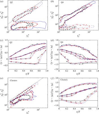
Figure 11. (a,b,e) Probability density functions of the wall-normal height of births, $y_{b}$ (——), and deaths, $y_{d}$ (- - - -), of tall attached primary branches, as a function the mean height of their centre of gravity, $y_{c}$ . The dashed straight line is $y_{b,d}=2y_{c}$ . (c,d,f) Probability density functions of the minimum (- - - -) and maximum (——) heights of tall attached primary branches, as functions of the time elapsed from their birth. Time is normalized with the lifetime of each branch, $T$ , and $y_{min}$ and $y_{max}$ with the heights, $y_{b}$ and $y_{d}$ , at its birth and death, respectively (see figure 10). The solid horizontal lines are the average position of the wall. (a,c) Ejections. (b,d) Sweeps. (e, f) Vortex clusters. In all cases, each vertical section is a p.d.f., and the contours are 0.5 of its maximum. Symbols as in table 1.

The evolution of the maximum and minimum structure heights during the life of a branch is given in figure 11(c,d). As we just saw, the Q2s are born attached to, or very near, the wall. They remain attached for approximately ${\textstyle \frac{2}{3}}$ of their lives, after which they detach and rise quickly. Their maximum height grows steadily during that time. The evolution of the Q4s is the opposite. Their bottom moves down relatively quickly, attaches to the wall at roughly ${\textstyle \frac{1}{3}}$ of the branch live and stays attached thereafter. Their top moves down steadily. The details of the distribution into attached and detached behaviour change slightly when considering very tall branches, or those closer to the buffer layer, but the overall behaviour is always just as described. Clusters behave approximately as Q2s, although, as already mentioned, their range of heights is more limited (figure 11 e, f).

The wall-normal velocity of the individual eddies is shown in figure 12(a,b), defined from the vertical displacement of their centre of gravity between consecutive times separated by ${\rm\Delta}t^{+}\approx 30$ (to avoid spatial and temporal resolution issues) during which merging or splitting is not taking place. Consistent with the previous discussion, ejections move upwards on average, and sweeps move towards the wall, and it is interesting that both move within fairly narrow ranges of wall-normal velocities close to $\pm u_{{\it\tau}}$ . This agrees with the results of Flores & Jimenez (Reference Flores and Jiménez2010), who noted that strong sweeps and ejections in a small channel move across the logarithmic layer with surprisingly constant velocities. Note that these velocities are also consistent with a total vertical excursion of order $l_{y}$ (figure 11 a,b) during a lifetime of order $l_{y}/u_{{\it\tau}}$ (figure 9 b). Vortex clusters have both positive and negative vertical velocities. Apparently, although most clusters follow ejections as they rise, some of them also move with the sweeps as they drop. The shapes of the velocity distributions do not depend much on the attached or detached character of the structures being tracked, although the velocities decrease somewhat in the buffer layer, as expected (not shown).

Figure 12. Probability density functions of the wall-normal velocity of the centre of gravity of the structures. The vertical lines are $\text{d}y_{c}/\text{d}t=\pm u_{{\it\tau}}$ in (a) and $\text{d}y_{c}/\text{d}t=0$ in (b). (a) ——, Ejections; - - - -, Sweeps. (b) Vortex clusters. Symbols as in table 1.

It was speculated by Flores & Jimenez (Reference Flores and Jiménez2010) that bursts and ejections are parts of a single underlying structure, because they tend to burst and ebb concurrently in channels whose dimension has been adjusted to be minimal in the logarithmic layer, and also because their symmetric vertical velocities suggest a common cause. It is also known that they tend to occur in side-by-side pairs (Lozano-Durán et al. Reference Lozano-Durán, Flores and Jiménez2012) and that the conditional mean flow field of such pairs is a large-scale streamwise roller whose up- and down-welling edges contain the $\text{Q}^{-}$ s, both in the buffer layer (Guezennec et al. Reference Guezennec, Piomelli and Kim1989) and farther from the wall (Jiménez Reference Jiménez2013b ). The symmetry of the distributions in figures 9(c) and 12(a) further supports that view.

5.3. Relative position of branch creation

We next consider whether the birth of new tall attached branches is influenced by pre-existent structures in their neighbourhood, such as would be the case, for example, in the vortex-packet propagation mechanism proposed by Tomkins & Adrian (Reference Tomkins and Adrian2003). Note, however, that such an association would not necessarily imply causation, and could rather be due to the presence of a larger undetected common structure, as discussed above.

For that purpose, we look at the location with respect to existing structures of the birth of branches that will eventually become tall attached. At each moment, a frame of reference is defined at the centre of gravity of existing tall attached structures, and the relative positions of births taking place at that moment are computed. Figure 13 sketches the procedure. The relative distances are defined as

where $x_{c}$ and $z_{c}$ are the coordinates of the centre of the existing structure, and $x_{b}$ and $z_{b}$ the position of the newborn one. The distances are normalized with the length of the $x$ – $z$ diagonal of the circumscribed box of the existing structure, and only births between the wall and the maximum height of the existing structure are considered.

Figure 13. Sketch of the relative streamwise and spanwise distances of births with respect to existing tall attached structures. Points $(x_{c},z_{c})$ and $(x_{b},z_{b})$ are the wall-parallel coordinates of the centres of gravity of the existing and newborn structures, respectively.

The resulting p.d.f.s are shown in figure 14(a–d). In all cases, the central part of the p.d.f.s has a low probability of finding births, because that region is already occupied by the existing structure. Figure 14(a,b) show that existing ejections trigger new ejections ahead of themselves, while existing sweeps trigger new sweeps predominantly behind. The p.d.f.s of the relative wall-normal position of births (not shown) reveal that the new ejections tend to appear in the buffer layer (consistently with figure 11(a)) whereas sweeps are born roughly at the same height as the centre of gravity of the already existing ones. Figure 14(c) displays the birth of sweeps with respect to existing ejections, and a symmetric figure can be drawn for ejections with respect to sweeps. It shows that Qs of different quadrants are not created aligned to each other, but side by side. Note that, in this case, the probability map is oriented in such a way that the closest newborn structure is always to the left ( ${\it\delta}_{z}>0$ ) of the existing one. An un-oriented p.d.f. would show new structures appearing symmetrically at both sides of the centre. Note also that, for that reason, the minimum birth probability of this case is not at the centre of the p.d.f. but to its right ( ${\it\delta}_{z}<0$ ). Births in that location have been transferred to the peak on the left ( ${\it\delta}_{z}>0$ ). Finally, figure 14(d) shows that vortex clusters are born downstream of existing ones, as in the case of ejections.

Figure 14. Joint probability density functions of the relative streamwise, ${\it\delta}_{x}$ , and spanwise, ${\it\delta}_{z}$ , distances of births with respect to existing tall attached structures whose height is ${\it\Delta}_{y}^{+}\geqslant 200$ (see sketch in figure 13). (a) New ejections with respect to existing ejections. (b) New sweeps with respect to sweeps. (c) New sweeps with respect to ejections. (d) New vortex clusters with respect to existing clusters. Contours are 1.2 (——) and 0.8 (- - - -) the probability in the far field. Symbols as in table 1.

The p.d.f.s in figure 14 are self-similar plots normalized with the size of the ‘parent’ structure, and therefore have no absolute dimensions associated with them. If we consider them as reflecting a causal relation, they show that larger structures influence regions farther from their centres than small ones do. The p.d.f.s in figure 14 are highly reminiscent of the p.d.f.s of the relative location of neighbouring structures in figure 11 of Lozano-Durán et al. (Reference Lozano-Durán, Flores and Jiménez2012), including similar distances between the different peaks, suggesting that the geometric relations between existing structures reflect their process of formation. We have already mentioned that Q2s and Q4s are organized into streamwise trains of pairs each of which contains a Q2 and a Q4 side by side, which can be interpreted to mean that sweeps and ejections are reflections of quasi-streamwise large-scale rollers, embedded in the longer streaks of the streamwise velocity; sweeps in the high-velocity side of the streak, and ejections in the low-speed part. Figure 14(c) and its counterpart in Lozano-Durán et al. (Reference Lozano-Durán, Flores and Jiménez2012) would then reflect the spanwise separation between the high- and low-velocity component of the streaks. The streamwise separation in figure 14(a,b) would correspond to the streamwise wavelength of the inhomogeneity of the streak, which is known to take predominantly the form of meandering, both near the wall (Jiménez et al. Reference Jiménez, del Álamo and Flores2004) and in the logarithmic layer (Hutchins & Marusic Reference Hutchins and Marusic2007).

However, the front-to-back asymmetry in figure 14(a,d) provides additional information beyond that contained in the relative position of the instantaneous structures. It shows that trains of ejections and clusters grow streamwise by extending downstream, but that sweeps grow towards their backs. This difference is difficult to interpret, since it was shown by Lozano-Durán et al. (Reference Lozano-Durán, Flores and Jiménez2012) that there are very few unpaired $\text{Q}^{-}$ s in the channel, and the Q4s triggered behind the pre-existing Q4 in figure 14(b) would eventually require the formation of new Q2s, and vice versa. It is not clear from figure 14(a) where those Q2s are coming from. Some possibilities suggest themselves, although they are unfortunately difficult to test statistically. The simplest one is probably that the pairs are completed by untriggered structures. The probability contours in figure 14 are only 20 % higher or lower than the uniform background probability of finding a newborn structure anywhere, but it is difficult to see why only one component of the organized pairs in figure 14(c), or in Lozano-Durán et al. (Reference Lozano-Durán, Flores and Jiménez2012), should be created randomly. A more likely possibility is that the missing trailing Q2s are created too far from the origin to show in figure 14(a). A plausible variant of that scenario starts by assuming that the triggering Q2s and Q4s are always in the form of pairs. They would also trigger new pairs, but only (or predominantly) with the opposite orientation to that of the existing one. A triggering Q2 from 14(a) with a Q4 to its right would create ahead of itself a new Q2 with a Q4 to its left, which would be too far from the existing Q4 to appear in the conditional probability distribution in 14(b). A similar scenario would account for the formation of a companion Q2 for the new Q4 in figure 14(b). Thus, a clockwise quasi-streamwise roller, with the sweep to the right of the ejection (see figure 9 in Jiménez Reference Jiménez2013b ) would only trigger anticlockwise rollers ahead or behind itself. This process would not be too different from the self-propagation of hairpin packets in Tomkins & Adrian (Reference Tomkins and Adrian2003), although it should be made clear that the objects being discussed here live predominantly in the logarithmic layer, and that none of the evidence in this paper, or in the companion one by Lozano-Durán et al. (Reference Lozano-Durán, Flores and Jiménez2012), suggests the presence of hairpins in that region. Note that the generation of rollers of alternating sign along a streak leads naturally to the observed streak meandering. It also agrees with the staggered-vortex models proposed by Schoppa & Hussain (Reference Schoppa and Hussain2002) for the buffer layer, and with the majority of the equilibrium and periodic exact solutions more recently found in wall-bounded flows, and reviewed, for example, by Kawahara et al. (Reference Kawahara, Uhlmann and van Veen2012).

5.4. Advection velocities

How structures deform during their evolution, and presumably what determines their lifetime, is in part controlled by the vertical gradient of their advection velocity. It is well-known that most flow variables advect roughly with the local mean streamwise velocity (Kim & Hussain Reference Kim and Hussain1993; Krogstad et al. Reference Krogstad, Kaspersen and Rimestad1998), and are thus deformed by the mean shear.

Figure 15. Probability density functions of the streamwise advection velocities of wall-parallel sections of the individual structures, as functions of their wall-normal distances. (a) Phase velocity. ——, Q2s; - - - -, Q4s. (b) Phase velocity. Vortex clusters. Symbols as in table 1. $+$ , advection velocity of the swirling coherent structures adapted from figure 10(b) of LeHew et al. (Reference LeHew, Guala and McKeon2013). (c) Phase velocity. Q2s in M4200. ○, all structures; $\times$ , ${\it\Delta}_{y}^{+}>400$ ; ▫, ${\it\Delta}_{y}^{+}>1000$ . (d) As in (c), but group velocity. In all panels, each horizontal section is a p.d.f., and contours are 40 % of its maximum. The thicker dashed line is the mean streamwise velocity profile for case M4200.

In this paper, the advection velocity of the wall-parallel sections of the structures is measured in two independent ways. In the first, the set of points within the section of the structure is correlated between consecutive times separated by ${\rm\Delta}t^{+}\approx 10$ (to avoid grid resolution issues), and the velocity is estimated from the shift away from the origin of the maximum correlation peak (Kuglin & Hines Reference Kuglin and Hines1975; Sutton et al. Reference Sutton, Wolters, Peters, Ranson and McNeill1983). This is the method typically used in PIV (Willert & Gharib Reference Willert and Gharib1991). The second method tracks the centre of gravity of the circumscribing rectangle to the section of the structure. Both velocities need not coincide if, for example, the structure moves by accreting new elements from the front and shedding them from behind. The difference is akin to the distinction of phase and group velocity in wavepackets, with the correlation method representing the phase velocity. Non-dispersive structures in which the phase and group velocities coincide can be considered as ‘coherent’ objects advected by the flow, while dispersive ones are probably better understood as being ‘footprints’ continuously destroyed and reformed by some global influence, such as pressure.

The results are shown in figure 15(a,b), which displays phase velocities from snapshots not involved in mergers or splits. All structures move approximately with the mean profile above the buffer layer. Ejections move slightly more slowly, roughly by $-1.5u_{{\it\tau}}$ , while sweeps move faster by roughly the same amount. This agrees with previous results (Guezennec et al. Reference Guezennec, Piomelli and Kim1989; Krogstad et al. Reference Krogstad, Kaspersen and Rimestad1998), and with the idea that ejections live in low-velocity streaks, and sweeps in high-velocity streaks. Vortex clusters can be either faster or slower than $U(y)$ , although the latter is slightly more probable, presumably reflecting their preferential association with ejections. This was also seen in their vertical velocities in figure 12(b). Their mean advection velocity is $U(y)-0.8u_{{\it\tau}}$ . Close to the wall, all structures advect roughly at $10u_{{\it\tau}}$ , in agreement with Kim & Hussain (Reference Kim and Hussain1993) and Krogstad et al. (Reference Krogstad, Kaspersen and Rimestad1998). Figure 15(b) also includes the p.d.f.s of the advection velocities reported by LeHew et al. (Reference LeHew, Guala and McKeon2013) which shows shorter tails although reasonable considering the differences between both methods. Elsinga et al. (Reference Elsinga, Poelma, Schröder, Geisler, Scarano and Westerweel2012) observed a mean advection velocity of $0.78U_{e}$ at $y=0.2h$ , with $U_{e}$ the free-stream velocity of the boundary layer, which also agrees with the value of $0.776U_{c}$ obtained for vortex clusters at $y=0.2h$ in the present study, being $U_{c}$ the mean channel velocity at the centreline.

On the other hand, these results are not entirely consistent with those of del Álamo & Jiménez (Reference del Álamo and Jiménez2009), who showed that large structures with wavelengths ${\it\lambda}_{x}\gtrsim 2h$ advect at all heights with the bulk velocity of the mean profile, including near the wall, where that velocity is very different from the local one. Their method computes a phase velocity, and this dependence on the wavelength suggests that, at least for large attached structures near the wall, turbulence should be dispersive. The same conclusion could be drawn from the attached-eddy model of Townsend (Reference Townsend1961), who proposed that large structures near the wall are passive (‘inactive’), controlled by active cores farther away from the wall. Bradshaw (Reference Bradshaw1967) later showed that the interaction between the outer active part and the inactive inner one was most likely due to the pressure induced by the active cores. This was even more vividly shown by Tuerke & Jiménez (Reference Tuerke and Jiménez2013) by means of a numerical experiment in which the $y$ -distribution of the total tangential stress in a channel was modified by a distribution of volume forces. They expressed the average stress at a given distance from the wall as a $y$ -dependent friction velocity, $u_{{\it\tau}}(y)$ , and showed that, while the intensity of the velocity fluctuation spectrum $k_{x}E_{uu}({\it\lambda}_{x},y)$ , where $k_{x}=2{\rm\pi}/{\it\lambda}_{x}$ , scale with $u_{{\it\tau}}^{2}(y)$ for relatively short wavelengths, ${\it\lambda}_{x}\approx y$ , the longer wavelengths scale everywhere much better with $u_{{\it\tau}}^{2}$ at the height of the active cores, $y={\it\lambda}_{x}/10$ . The suggestion in all of these cases is that, while the smaller scales contained within the attached root of a large structure may move approximately with the local mean velocity, the structure itself should advect with a velocity closer to that of the active core near its centre of gravity. For a graphic representation of this process, see the different behaviours of the root and body of the structure in figure 5(c). Note that this observation reinforces and refines the evidence for the modulation of the inner layer by the outer one documented by Mathis, Hutchins & Marusic (Reference Mathis, Hutchins and Marusic2009).

This is confirmed in figure 15(c,d), which show the advection velocity separately for structures of three different size ranges. Figure 15(c), shows the phase velocity as a function of $y$ . All of the size ranges agree, showing that the motion of the small scales traced by the correlation method is indeed independent of the size of their ‘host’ structure. On the other hand, the group velocities in 15(d), computed by tracking the circumscribing box, depend on the structure size. All of the structures travel with the mean velocity for $y^{+}\gtrsim {\it\Delta}_{y}/4$ , but they decouple from the mean flow below that level, and move with what can be interpreted as the advection velocity of the base of the active part of the structure. Note that, since both the shear time, $(\partial _{y}U)^{-1}\sim {\it\kappa}y/u_{{\it\tau}}$ , and the local eddy-turnover time, $y/u_{{\it\tau}}$ , decrease as we approach the wall, such a decoupling between the top and bottom parts of the attached structures, with very different local time scales, should probably have been expected.

The conclusion that only the upper part of the tall attached structures can be considered as coherent is interesting, because the lifetime of a structure is most probably limited by its deformation by the shear. Whenever a structure is sheared by much more than its length, it should disappear as a coherent object. The difference between the phase velocities at the top and bottom of an attached structure is approximately ${\rm\Delta}U\approx u_{{\it\tau}}{\it\kappa}^{-1}\log {\it\Delta}_{y}^{+}$ , which would shear it by an amount roughly equal to its length in a time of the order of ${\it\Delta}_{x}/{\rm\Delta}U\sim {\it\Delta}_{x}/(u_{{\it\tau}}\log {\it\Delta}_{y}^{+})$ . This estimate differs from the data in § 5.1 by the non-trivial logarithmic denominator. On the other hand, if the only deformation that counts is that between $y={\it\Delta}_{y}$ and $y={\it\Delta}_{y}/4$ , or some other constant factor, the shear time would be proportional to $({\it\Delta}_{x}/u_{{\it\tau}})\log 4$ , which agrees better with the observations.

6.1. Graphs

The discussion in the previous sections deals mostly with primary branches. Here we describe the behaviour of the secondary branches that interact with them. The underlying goal is to describe, if possible, the inertial cascade as a spatially localized process in which individual eddies merge and split, as implied in the original descriptions by Richardson (Reference Richardson1920) and Obukhov (Reference Obukhov1941), rather than simply as the conceptual scale-by-scale model introduced by Kolmogorov (Reference Kolmogorov1941). Our tool will be the identification of such interactions within the organization of the structures into branches and graphs.

As discussed in § 4, graphs are collections of branches that interact with each other at some point in their life. It is difficult to define unique descriptors for the geometry of the graphs, which can be quite complex objects (see figure 5 a,b), but they can be classified in the same way as branches. For example, a graph is tall attached if that is the case for at least one of the structures in one of its branches. For the same reasons as in the case of structures and branches, graphs can be given a unique type. For example, a Q2 graph is exclusively formed by Q2 structures, and there are no mixed graphs.

Figure 16 shows the normalized histogram of the number of branches per graph, and gives an idea of their complexity. The mode of the histogram is located at one branch per graph, but these cases correspond to simple small structures that evolve without splitting or merging. On the other hand, the tails of the histograms include large graphs with thousands of branches which represent groups of eddies (either Qs or clusters) that merge and split often, as in the example in figure 5(a).

Figure 16. Probability density functions of the number of branches per graph. Open symbols for $\text{Q}^{-}$ s and closed ones for vortex clusters. Symbols as in table 1 with squares for case M4200. The dashed line is proportional to $N^{-3}$ .

Graphs are mostly made of primary, incoming and outgoing branches, with very few connectors (see the classification in figure 6 and the discussion in § 3). When incoming and outgoing branches are considered, the results obtained in previous sections are little affected for detached and buffer-layer branches, but those for tall attached ones change. Roughly 60–70 % of the tall attached branches are secondary (either incoming or outgoing). Their evolutions are truncated versions of the tall attached primaries, with lifetimes biased towards shorter values and of the order of $l_{y}/(2u_{{\it\tau}})$ , which is half of that obtained for primaries. Their minimum and maximum wall distances (not shown) behave like those presented for primary branches in figure 11(c,d, f) but only until they interact (merge or split) with a primary. Hence, the equivalent plots for incoming branches are similar to the first half of figure 11(c,d, f) from $t/T=0$ (when they are born) to $t/T\approx 0.5$ (when they merge with a primary), whereas the plots for outgoing branches resemble the second half, from $t/T\approx 0.5$ (when they split from a primary) to $t/T=1$ (when they die).

6.2. Cascades

Figure 17 contains sketches of the two basic interactions among branches, and defines the notation for this section. Each elementary interaction involves three objects. Two of them, $b$ for big and $m$ for medium, are part of the main branch involved in the interaction, while the third ( $s$ for small) is the fragment being lost or gained. Thus, in the split in figure 17(a), a structure of characteristic size ${\it\Delta}_{b}$ breaks into a fragment of size ${\it\Delta}_{m}$ , which continues the branch, and loses a fragment of size ${\it\Delta}_{s}$ . We will call this interaction a direct cascade event. Similarly, in the inverse cascade event in figure 17(b), two structures of sizes ${\it\Delta}_{m}$ and ${\it\Delta}_{s}$ merge into a single one of size ${\it\Delta}_{b}$ . In both cases, the notation is $(b)\rightleftharpoons (s)+(m)$ . Usually, but not always, ${\it\Delta}_{b}>{\it\Delta}_{m}>{\it\Delta}_{s}$ . Note that the sketches in figure 17 depict the merger or split of a single structure at a given moment, but that it is fairly common to find several mergers or splits, or a mixture of them, coinciding in a single event.

Figure 17. Sketch of the process of: (a) split or direct cascade and (b) merge or inverse cascade. The structures labelled as $b$ (big) and $m$ (medium) belong to the same branch, and that denoted by $s$ (small) is the fragment that has split or merged.

For the purpose of characterizing interactions, we use as eddy size the length, ${\it\Delta}$ , of the three-dimensional diagonal of its circumscribing box, which is, on average, 1.3 times larger than the streamwise length. This choice was preferred instead of other lengths based on the volume of the structures due to their complicated shapes (see, for example, figure 2). For that reason, the split of a structure in two fragments with similar characteristic lengths as defined above do not necessarily imply similar volumes. The length ${\it\Delta}$ can be generalized to branches by averaging over the branch life, $l=\langle {\it\Delta}\rangle _{B}$ , as in § 4. When normalizing it with the Kolmogorov scale, we use the channel average at the height of the centre of gravity of the branch.

Also, since very few differences were found in the cascade statistics of sweeps and ejections, they are treated together for the rest of this section.

We analyse first the prevalence of interactions. Figure 18(a) shows the fraction of primary vortex-cluster branches that split or merge at least once in their lives, as a function of their mean diagonal length. There is a minimum size, $l\approx 30{\it\eta}$ , roughly agreeing with the peak of the energy-dissipation spectrum at ${\it\lambda}_{x}\approx 40{\it\eta}$ (Jiménez Reference Jiménez2012), below which branches rarely merge or split. In this range, the cascade is presumably inhibited by viscosity, and graphs contain a single branch that evolves without splitting or merging. On the other hand, almost all of the branches larger than $l\approx 100{\it\eta}$ , most of which are tall attached, merge or split at least once. In the transition between these two limits, the direct cascade predominates, and some branches split but never merge. Similar results are obtained for $\text{Q}^{-}$ s (not shown), although with less-pronounced differences between the direct and the inverse cascades. The buffer layer branches are excluded from the figure 18(a). They cascade very little and, when they are included in the figure, the cascading fractions increase more slowly and the curves move to the right, reaching unity at $l\approx 180{\it\eta}$ .

Figure 18. (a) Fraction, $f$ , of the number of primary clusters branches that split (——) or merge (- - - -) at least once in their lives, as a function of the mean diagonal length of the branch, $l$ . The buffer layer branches are excluded. The vertical dashed lines are $l=30{\it\eta}$ and $l=100{\it\eta}$ . Symbols as in table 1. (b) Ratio between the volume of direct and inverse cascade as a function of the Reynolds number. $\Box$ , $\text{Q}^{-}$ s; $\times$ , vortex clusters.

Next, we characterize the part of the growth and decay of the structures that is due to mergers and splits, which can be interpreted as a measure of the contribution of the inverse and direct cascades to the eddy evolution. To do that, we compare the total volume gained or lost by primary branches in their cascade interactions with the average volume of the branch, $V_{b}$ . For example, the total lost volume (direct cascade), $\sum _{B}V_{sd}$ , is defined as the sum of the volumes of all of the fragments lost during the life of the branch, with a similar definition for the volume gained, $\sum _{B}V_{si}$ . Excluding the buffer layer branches, Q primaries with $l>100{\it\eta}$ have on average $\sum _{B}V_{sd}/V_{b}\approx 0.72$ and $\sum _{B}V_{si}/V_{b}\approx 0.50$ for case M4200. For vortex clusters, the ratios are on average 1.41 and 0.73. In both cases mergers and splits are substantial contributors to the eddy growth and decay.

The ratio

gives an idea of which of the two cascades dominates in a given branch. Its average, $\langle r_{B}\rangle$ , is plotted in figure 18(b) for different Reynolds numbers and branch types. The direct cascade always dominates, especially for vortex clusters, and its dominance increases slightly with the Reynolds number. However, the imbalance is not huge, approximately 1.3 for $\text{Q}^{-}$ s and 2.2 for vortex clusters, implying that the inverse cascade is not negligible, in accordance with the backscatter observations of Piomelli et al. (Reference Piomelli, Cabot, Moin and Lee1991) and others.

To understand better how this imbalance is distributed as a function of scale, we decompose the ratio $r_{B}$ in terms of the size of the fragments involved, $r$ . Figure 19(a) shows the ratio $r({\it\Delta}_{s},\,{\it\Delta}_{b})$ , defined as in (6.1) but restricting the sums and the subsequent averaging to interactions involving a smallest and largest eddy of those sizes. The figure refers to vortex clusters in case M4200, but qualitatively similar ones are obtained for $\text{Q}^{-}$ s and for vortex clusters at different Reynolds numbers.

Figure 19. (a) Volume ratio between the direct and inverse cascades, as a function of the sizes of the smallest and largest fragments in a given interaction. Vortex clusters in M4200. The dashed line is ${\it\Delta}_{s}=0.4{\it\Delta}_{b}$ . Contours are, from dark to light, 3.5, 3, 2.5, 2 and 1.2. (b) Probability density functions of the sizes of the fragments merged (- - - -) or split (——), ${\it\Delta}_{s}$ , for different lengths of the larger eddy involved, ${\it\Delta}_{b}/{\it\eta}=0$ –200, 200–500, 500–2000. Data for vortex clusters. The vertical dashed line is ${\it\Delta}_{s}=30{\it\eta}$ . Symbols as in table 1.

The direct cascade always prevails, but the imbalance is strongest along a ridge ${\it\Delta}_{s}\approx 0.4{\it\Delta}_{b}$ , which corresponds to eddies splitting roughly in halves, or merging with others of similar size. It is also strongest for small structures below ${\it\Delta}_{b}\approx 60{\it\eta}$ , which tend to split in fragments of ${\it\Delta}_{s}\approx 20{\it\eta}$ much more frequently than they merge. This ridge can be interpreted as the preferred locus of a predominantly direct cascade, but note again that the imbalance for inertial structures is at most a factor of two, and that the cascade only really becomes unidirectional when one of the fragments is small enough to be dissipated by viscosity.

Figure 19(b) studies in more detail the merging or splitting process by presenting the p.d.f.s of the size of the smallest structure involved in an interaction for different ranges of the size of largest one. Most of the fragments are of the order of ${\it\Delta}_{s}\approx 30{\it\eta}$ , corresponding to viscous fragments torn from larger eddies or merging into them. However, the tails of the p.d.f.s get longer as the largest structure gets bigger, representing inertial interactions between eddies of comparable sizes. Further analysis of the data (not shown) confirms this trend, and reveals that the size of the largest fragment likely to merge into, or split from, an eddy of size ${\it\Delta}_{b}$ is some fixed fraction of ${\it\Delta}_{b}$ . Note that the p.d.f.s in figure 19(b) are almost identical for mergers and splits, and that the previous discussion applies equally well for the direct as for the inverse cascade.

The temporal behaviour of the two cascades is studied in figure 20. Figure 20(a) shows the average time, $T_{I}$ , elapsed before a $\text{Q}^{-}$ of size ${\it\Delta}_{b}$ splits into two similar fragments, or a $\text{Q}^{-}$ of size ${\it\Delta}_{m}$ merges with another one of similar size (in both cases defined as $|{\it\Delta}_{m}-{\it\Delta}_{s}|<0.1{\it\Delta}_{m}$ ). This time may be interpreted as characterizing the inertial cascade and it is defined as the time elapsed between the birth of a primary and its first roughly symmetrical split or merger at sizes ${\it\Delta}_{b}$ or ${\it\Delta}_{m}$ , respectively. In the case of several such events in a single branch, we consider $T_{I}$ as the time between two consecutive inertial interactions, with the sizes ${\it\Delta}_{b}$ and ${\it\Delta}_{m}$ belonging to the last one. The results show that $T_{I}^{+}\approx 0.35{\it\Delta}_{m,b}^{+}$ for both merging and splitting, and a further analysis reveals that primaries with $l>100{\it\eta}$ undergo two or three inertial events in its life, counting mergers and splits. In general, if we count any interaction regardless of its size, the average number of splits (or mergers) in a branch is $n\approx 10^{-4}(l/{\it\eta})^{2}$ for primaries with $l>100{\it\eta}$ and excluding the buffer layer branches.

Figure 20. (a) Average time, $T_{I}$ , for a $\text{Q}^{-}$ to merge with, or split into, two fragments of similar size $(|{\it\Delta}_{m}-{\it\Delta}_{s}|/{\it\Delta}_{m}<0.1)$ , plotted against ${\it\Delta}_{m}$ for mergers and ${\it\Delta}_{b}$ for splits. ——, splitting; - - - -, merging. The dashed-dotted line is $T_{I}^{+}=0.35{\it\Delta}_{m,b}^{+}$ . Data for primary branches. (b) Probability density functions of the time at which mergers and splits take place, normalized with the branch lifetime. ——, splits, - - - -, mergers. Primary tall attached $\text{Q}^{-}$ s. Symbols as in table 1.

Figure 20(b) shows that mergers and splits are asymmetrically distributed during the life of the branch. While splits happen at the end of the life, and contribute to tear the structure apart, mergers take place at the beginning and enhance the early stages of the growth of the eddy. While the figure is drawn for $\text{Q}^{-}$ s, similar results are obtained for vortex clusters.

Figure 21. Sketch of the relative position of the centre of gravity of fragments merged or split (structure $s$ ) with respect to the centre of gravity of the medium eddy (structure $m$ ).

Figure 22. Joint probability density functions of the relative wall-normal and streamwise distances of the centres of mergers and splits (structures $s$ ) with respect to the centre of the medium eddy (structure $m$ ) normalized with the characteristic size of the latter,  $l_{m}$ . See the sketch in figure 21. Contours are 20 and 90 % of the data. (a) Splits for $\text{Q}^{-}$ s. (b) Mergers for $\text{Q}^{-}$ s. (c) Splits for vortex clusters. (d) Mergers for vortex clusters. Symbols as in table 1.

Finally, the spatial organization of mergers and splits is studied in figure 22 by looking at the relative position of the centre of gravity of the smallest fragment with respect to the intermediate one (see the sketch in figure 21). Figure 22(a,b) show results for $\text{Q}^{-}$ s. Most of the mergers and splits take place in the streamwise direction. The structures merge predominantly with fragments below and ahead of them, presumably because taller and faster structures overtake smaller ones. The splits occur mostly in the tail of the structure or in its upper-front head. Since we saw in § 5.4 that tall attached $\text{Q}^{-}$ s are tilted forward by the shear, this distribution of splits seem to reflect the occasional tearing of their heads and tails during that process. The results for vortex clusters are not as interesting (figure 22 c,d). Most of their interactions take place near the core of the original structure. The reason is probably that vortex clusters are much ‘emptier’ than $\text{Q}^{-}$ s (see figure 2, and Lozano-Durán et al. Reference Lozano-Durán, Flores and Jiménez2012), and there is enough space within them for mergers and splits to happen internally.

With respect to the nature of the participants in an interaction, tall attached structures split 68 % of the time into another tall attached structure and either a detached or a short attached one. In 25 % of the interactions, neither of the resultant structures is tall attached, while only in 7 % of the cases both of them are. Similar results are obtained for mergers and vortex clusters at different Reynolds numbers in this respect.

Taking the evidence in this section at face value, it is difficult not to think of the classical interpretation of the cascade by Leith (Reference Leith1967) or Orszag (Reference Orszag1970), according to which the inertial energy transfer is an entropy-driven random process in phase space, in which energy tends to equipartition while drifting either up or down in scale (see the discussion in Lesieur Reference Lesieur1991, pp. 295–305). It is only when viscosity breaks the energy conservation at the smallest scales that the energy is unidirectionally drained into heat. However, there are two important caveats.

The first was already mentioned in the introduction. It should be clearly understood that most of the results in this section refer to the large scales in which energy is being fed into any possible inertial cascade. This should be clear from their association with the tangential Reynolds stress, and from the observation in figure 8 that the attached structures are larger that the Corrsin scale, and therefore directly coupled with the mean shear. As such, although the cascade process described in this section is probably a good description of how the momentum transfer changes scale across the logarithmic layer, it may not be representative of the behaviour of the, presumably universal, Kolmogorov (Reference Kolmogorov1941) inertial energy cascade.

In the second place, the description of a structure gaining fragments from its front (or back) while shedding them from the other end, could be interpreted as the definition of a dispersive wavepacket, and it was shown in § 5.4 that the bottom part of the attached structures is dispersive. To test whether this could be a simpler interpretation of the ‘reversible’ cascade described here, the objects from case M2000 were recomputed and tracked again after discarding all the planes for which $y^{+}<100$ . It follows from figure 15(d) that structures above that level are mostly non-dispersive. The results in this section were then recalculated. The new structures were indeed different from those including the buffer layer. For example, the average structure size decreased somewhat, reflecting the loss of connectivity through the buffer layer, but no qualitative differences were found for the cascade statistics described here.