


1. Introduction
Natural convection flows in heated square enclosures is a classic heat transfer problem and has drawn significant interest due to the relevance of this phenomena in engineering applications and the natural world, and have been studied in the context of heat exchangers (Chen & Chou Reference Chen and Chou2006), solar energy collection (Sharma, Chen & Lan Reference Sharma, Chen and Lan2009), ice formation (Inaba & Fukuda Reference Inaba and Fukuda1984) and oceanic flows, to name a few. The imbalance between viscous and buoyancy forces drives the fluid motion and heat transport, and the onset of unsteadiness and eventual transition to turbulence remains a widely investigated topic even after decades of research, as they are pivotal in developing a deeper understanding in this field.
The problem of natural convection in a differentially heated square cavity with conducting vertical walls and adiabatic horizontal walls was first popularized by de Vahl Davis (Reference de Vahl Davis1983) through a benchmark numerical solution. He addressed the mesh dependence of a second-order, central difference approximation, and obtained solutions for heat flux, temperature and velocities at Rayleigh numbers up to  $10^{6}$. The effect of inclining these square enclosures garnered significant interest as it would break the static equilibrium in an otherwise stratified medium. Wunsch (Reference Wunsch1970) and Phillips (Reference Phillips1970) independently presented findings regarding the effect of inclination on natural convection within confined enclosures in the context of sloping ocean floors. They concluded that an insulated boundary in a stratified medium can induce up-slope flow when inclined to the horizontal, as a result of local bending of isotherms normal to the insulating boundary to maintain the no-flux condition. Peacock, Stocker & Aristoff (Reference Peacock, Stocker and Aristoff2004) provided experimental verification of the angular dependence of these natural convection flows, and determined the tilt angle corresponding to maximum fluid velocity, below which the velocity profile departs from that of the Phillips–Wunsch flow. Quon (Reference Quon1976) employed a finite difference method to study a differentially heated square cavity and the effects of tilting this enclosure from
  $0^\circ$ to
  $90^\circ$ to the horizontal. He concluded that flow solutions in corner regions held little significance with regard to the overall flow at smaller tilt angles. However, he was unable to obtain solutions at various angles due to numerical constraints. Page (Reference Page2011) presented solutions for the steady problem across a wider range of angles, overcoming the numerical complications encountered by Quon (Reference Quon1976), and reinforced his statement that flow in corner regions provided negligible contribution to the overall flow solution at smaller angles, though they become important for higher Prandtl number flows where corner-localized circulations appear. Grayer et al. (Reference Grayer, Yalim, Welfert and Lopez2020) studied the differentially heated square cavity with insulated vertical walls and conducting horizontal walls; they considered both steady and unsteady flows, and investigated the effects of tilting this configuration at angles ranging between 0
 $^\circ$ and 90
 $^\circ$ to the horizontal. The flow in their study was characterized by a buoyancy number
  $R_{N}$, which is taken as the square root of the Grashof number, and their investigations determined that the critical
  $R_{N}$ corresponding to two-dimensional instability decreases with increasing angle of inclination, with instability occurring through three distinct modes. The angular dependency of natural convection flows has also been investigated for a wide range of different configurations, such as cylindrical containers (Shishkina & Horn Reference Shishkina and Horn2016; Zwirner et al. Reference Zwirner, Khalilov, Kolesnichenko, Mamykin, Mandrykin, Pavlinov, Shestakov, Teimurazov, Frick and Shishkina2020), arrays of square cylinders (Al-Suhaibani, Ali & Almuzaiqer Reference Al-Suhaibani, Ali and Almuzaiqer2024), and partitioned rectangular enclosures (Acharya & Tsang Reference Acharya and Tsang1985; Kangni, Vasseur & Bilgen Reference Kangni, Vasseur and Bilgen1995), to name a few.
Various studies have examined the square enclosure in a fixed orientation, particularly the differentially heated configuration comprising conducting vertical walls and insulating horizontal walls (Ravi, Henkes & Hoogendoorn Reference Ravi, Henkes and Hoogendoorn1994; Janssen & Henkes Reference Janssen and Henkes1996; Le Quéré & Behnia Reference Le Quéré and Behnia1998; Oteski et al. Reference Oteski, Duguet, Pastur and Le Quéré2015; Wang et al. Reference Wang, Liu, Verzicco, Shishkina and Lohse2021), and the laterally heated configuration comprising adiabatic vertical walls and conducting horizontal walls heated from below, corresponding to the well studied Rayleigh–Bénard scenario (Rayleigh Reference Rayleigh1916).
Though the two-dimensional aspects of the heated square cavity problem have been investigated thoroughly, there has been significantly less coverage on the three-dimensional stability of these two-dimensional flows. Henkes & Le Quéré (Reference Henkes and Le Quéré1996) examined the differentially heated square cavity, and considered the stability of these flows to both two- and three-dimensional disturbances, concluding that the base flow is more unstable to three-dimensional disturbances than two-dimensional ones. Xin & Le Quéré (Reference Xin and Le Quéré2001) came to similar conclusions, but for the laterally heated square cavity. Adachi (Reference Adachi2006) evaluated the three-dimensional stability of natural convection flows in an inclined square duct of infinite length with boundary conditions corresponding to the Rayleigh–Bénard configuration, and considered the untilted problem and an inclination  $0.01^\circ$ to represent installation errors in industrial devices. This study concluded that above a critical Rayleigh number, the tilted scenario produces a two-dimensional longitudinal roll, whilst the untilted duct experiences three-dimensional transverse rolls. Torres et al. (Reference Torres, Henry, Komiya, Maruyama and Hadid2013) applied the same boundary conditions, but instead considered a duct of finite length and considered tilt angles up to
  $90^\circ$, and obtained the domain of these stable solutions in the Rayleigh number – inclination parameter space. Other studies have considered the three-dimensional flow scenario for a differentially heated square cavity (Fusegi et al. Reference Fusegi, Farouk, Hyun and Kuwahara1990; Wang, Zhang & Guo Reference Wang, Zhang and Guo2017; Zwirner et al. Reference Zwirner, Emran, Schindler, Singh, Eckert, Vogt and Shishkina2022).
In the present study, we investigate the configuration considered in Grayer et al. (Reference Grayer, Yalim, Welfert and Lopez2020), namely a square cavity with adiabatic vertical walls and a fixed temperature difference between the horizontal walls. The primary interest of the present study is to investigate the three-dimensional stability of the considered system, whereas Grayer et al. (Reference Grayer, Yalim, Welfert and Lopez2020) evaluated its two-dimensional stability. Here, two-dimensional solutions are extended to span inclinations from  $0^\circ$ to
  $180^\circ$, and a linear stability analysis is used to interrogate the stability of these flows to infinitesimal three-dimensional perturbations. Perturbation spatial structures are presented, and direct numerical simulations (DNS) are employed to both evaluate nonlinear effects and validate the linear stability analysis predictions.
The structure of this paper is as follows. The system under investigation, numerical scheme and results from the grid resolution study are presented in § 2. Characteristics of the two-dimensional base flow are described, and comparisons to published studies are presented for validation purposes, in § 3.1. The three-dimensional stability of the flow is discussed in §§ 3.3 and 3.4, describing the critical  $R_{N}$ corresponding to three-dimensional instability and its dependence on the inclination angle, and instability perturbation structures are discussed in § 3.5. Nonlinear effects of the three-dimensional transition are discussed in § 3.6, and conclusions are drawn in § 4.
2. Methodology
2.1. Problem formulation
The system under investigation is displayed in figure 1 and comprises a fluid contained in a square enclosure of length  $L$ inclined to the horizontal at an angle
  $\theta$ (measured in degrees). Enclosure inclinations between
  $0^\circ$ and
  $180^\circ$ are considered, increasing in the anticlockwise direction. For the untilted configuration (at
  $\theta =0^\circ$), the vertical walls are insulated, and the horizontal walls are conducting, with the top wall being hotter than the bottom wall (a stable stratification configuration); the no-slip condition is applied to all four walls. The fluid has kinematic viscosity
  $\nu$, volumetric thermal expansion coefficient
  $\beta$, and thermal diffusivity
  $k$. The Prandtl number characterizes the ratio of momentum diffusivity to thermal diffusivity and is given by
  $Pr=\nu /k$. In this study, the Prandtl number is held at
  $Pr=0.71$, corresponding to air at room temperature; this value is consistent with several previous square cavity studies (de Vahl Davis Reference de Vahl Davis1983; Fusegi et al. Reference Fusegi, Farouk, Hyun and Kuwahara1990; Xin & Le Quéré Reference Xin and Le Quéré2001; Grayer et al. Reference Grayer, Yalim, Welfert and Lopez2020). The top and bottom walls are held at fixed temperatures
  $T_{hot}$ and
  $T_{cold}$, respectively, such that
  $\Delta T=T_{hot}-T_{cold}>0$. Gravity
  $\boldsymbol {g}$ acts in the downwards vertical direction.

Figure 1. System configuration showing the enclosure tilted at angle  $\theta$, with a cold bottom wall and hot top wall represented by the blue and red lines, respectively.
The non-dimensional temperature is normalized as  $T=(T^*-T_{cold})/\Delta T-0.5$, with
  $T^*$ being the dimensional temperature. Length and time are respectively scaled by
  $L$ and
  $1/N$, where
  $N$ denotes the Brunt–Väisälä (buoyancy) frequency and is given by
  $N = \sqrt {\boldsymbol {g}\beta \,\Delta T/L}$. For convenience, a Cartesian coordinate system is established with its origin at the centre of the enclosure, such that the
  $x$-coordinate runs parallel to the conducting walls, and the
  $y$-coordinate runs parallel to the adiabatic walls. This non-dimensional reference frame is attached to, and rotates with, the enclosure. With the enclosure inclined at a anticlockwise angle
  $\theta$, a unit vector pointing in the upward vertical direction is given by
  $\boldsymbol {\xi } = (\sin \theta,\cos \theta )$, and the velocity field is
  $\boldsymbol {u}=(u,v)$. The four corners of the enclosure at
  $(x,y) = (-0.5,-0.5)$,
  $(x,y) = (0.5,-0.5)$,
  $(x,y) = (0.5,0.5)$,
  $(x,y) = (-0.5,0.5)$ will be respectively referred to as A, B, C and D, as illustrated in figure 1.
2.2. Governing equations
The two-dimensional base flow in this system is governed by the dimensionless Navier–Stokes equations under the Boussinesq approximation, which effectively ignores density variations except in the gravity term:
 $$\begin{gather} \boldsymbol{\nabla} \boldsymbol{\cdot} \boldsymbol{u}=0, \end{gather}$$
 $$\begin{gather}\frac{\partial \boldsymbol{u}}{\partial t}+(\boldsymbol{u} \boldsymbol{\cdot} \boldsymbol{\nabla})\boldsymbol{u}={-}\boldsymbol{\nabla} p + \frac{1}{R_{N}}\,\nabla^{2}\boldsymbol{u}+T\boldsymbol{\xi}, \end{gather}$$
 $$\begin{gather}\frac{\partial T}{\partial t}+(\boldsymbol{u} \boldsymbol{\cdot}\boldsymbol{\nabla})T = \frac{1}{Pr\, R_{N}}\,\nabla^{2}T, \end{gather}$$
where  $p$ denotes the reduced pressure, and the dimensionless buoyancy number given by
 \begin{equation} R_N=\frac{NL^{2}}\nu \end{equation}
represents the ratio of viscous and buoyancy forces. Under this non-dimensionalization, the hot and cold walls are held at dimensionless temperatures  $T_{hot}=0.5$ and
  $T_{cold}=-0.5$.
The system (2.1) and its boundary conditions imply that the base flow is skew-symmetric with respect to the centre of the enclosure, i.e.
 \begin{equation} (u,v,T)({-}x,-y)={-}(u,v,T)(x,y). \end{equation}
Following the terminology of Xin & Le Quéré (Reference Xin and Le Quéré2001), this state is taken to be centro-symmetric.
The Nusselt number represents the ratio of convective to conductive heat transfer and is generally used to quantify heat transfer in natural convection flows. Given that the temperature and length terms are dimensionless, the definition of the Nusselt number is taken as the dimensionless temperature flux along the hot and cold boundaries, which are given by
 $$\begin{gather} \textit{Nu}_h= \int_{{-}0.5}^{0.5} \frac{\partial T(x,0.5)}{\partial y}\,\mathrm{d}\kern0.07em x, \end{gather}$$
 $$\begin{gather}\textit{Nu}_c= \int_{{-}0.5}^{0.5} \frac{\partial T(x,-0.5)}{\partial y}\,\mathrm{d}\kern0.07em x. \end{gather}$$
Furthermore, the buoyancy number is related to the Rayleigh number through  $R_N = \sqrt {Ra/Pr}$. The problem definition, governing dimensionless parameter
  $R_{N}$ and (2.1a)–(2.1c) presented in this study, follows the nomenclature used in Grayer et al. (Reference Grayer, Yalim, Welfert and Lopez2020) as it represents the same system.
2.3. Numerical scheme and computational domain
For the two-dimensional base flows, the aforementioned Navier–Stokes equations are spatially discretized using a nodal spectral-element method (Karniadakis & Triantafyllou Reference Karniadakis and Triantafyllou1992) and evolved in time using a third-order backward differentiation scheme (Karniadakis, Israeli & Orszag Reference Karniadakis, Israeli and Orszag1991). The computational domain is first subdivided into quadrilateral macro-elements whereby a Lagrangian tensor-product polynomial shape function is imposed onto each element. The polynomials are interpolated at the Gauss–Legendre–Lobatto quadrature points within each element. These schemes are implemented using an in-house solver and have been validated previously in various studies (Sheard et al. Reference Sheard, Leweke, Thompson and Hourigan2007; Sheard, Fitzgerald & Ryan Reference Sheard, Fitzgerald and Ryan2009; Blackburn & Sheard Reference Blackburn and Sheard2010; Ng, Vo & Sheard Reference Ng, Vo and Sheard2018; Mayeli, Tsai & Sheard Reference Mayeli, Tsai and Sheard2022; Murali, Ng & Sheard Reference Murali, Ng and Sheard2022).
Solutions are obtained using the computational domain displayed in figure 2, which comprises 100 elements with polynomial order  $N_{P}=10$. Element density is biased towards the walls of the enclosure where significant flow behaviour and thin boundary layers are anticipated. A grid resolution study was conducted to ensure that the dynamics of the flow is sufficiently resolved.

Figure 2. The computational domain used in this study, showing (a) the macro-element distribution, and (b) the element distribution along with the interpolation points corresponding to the polynomial order  ${N_P=10}$.
Two enclosure inclinations were considered in this grid resolution study, namely  $\theta =30^\circ$ and
  $75^\circ$. Values for total kinetic energy and Nusselt number at the hot wall were computed at a buoyancy number
  $R_{N}=10^{4}$ as this is anticipated to be high enough for significant flow and boundary layer development. Results produced at
  $N_{P}=15$ using a 225-element mesh were used as a high-resolution reference case. As shown in table 1, all considered parameters converge to below 0.1 % relative error for
  $N_{P}\geq 10$. Therefore,
  $N_P = 10$ is used hereafter unless otherwise specified.
Table 1. Percentage errors with increasing  $N_P$ shown for kinetic energy (
 $E_k$) and Nusselt number at the hot wall (Nu
  $_h$) determined at
  $R_N=10^4$ for inclinations
  $\theta =30^\circ$ and
  $75^\circ$, relative to a high-resolution reference case obtained at
  $N_P=15$.

2.4. Linear stability analysis
Linear stability analysis is employed to investigate the stability of two-dimensional flows by taking  $(\bar {\boldsymbol {u}},\bar {p},\bar {T})$ as the solution of the two-dimensional base flow and imposing an infinitesimal three-dimensional perturbation field
  $(\boldsymbol {u}',p',T')$ upon it such that the velocity, pressure and temperature fields are given by
  $\boldsymbol {u}=\bar {\boldsymbol {u}}+\varepsilon \boldsymbol {u}'$,
  $p=\bar {p}+\varepsilon p'$ and
  $T=\bar {T}+\varepsilon T'$, respectively, for constant
  $\varepsilon$ satisfying
  $|\varepsilon |\ll 1$. Substituting these into (2.1a)–(2.1c) and retaining terms of order
  $O(\varepsilon )$ yields linearized equations for the evolution of infinitesimal three-dimensional perturbations
  $(\boldsymbol {u}',p',T')$. Spanwise homogeneity of the geometry permits a decomposition of the three-dimensional perturbation field into linearly independent Fourier modes,
 \begin{equation} (\boldsymbol{u}',p',T')(x, y, z, t) = \int_{-\infty}^{\infty} (\hat{\boldsymbol{u}},\hat{p},\hat{T})(x, y, m, t)\,\mathrm{e}^{\mathrm{i}mz}\, \mathrm{d}m, \end{equation}
where spanwise wavenumber  $m$ relates to the spanwise wavelength via
  $\lambda =2{\rm \pi} L/m$. The linearized equations for the evolution of an individual Fourier mode
  $(\hat {\boldsymbol {u}}_m,\hat {p}_m,\hat {T}_m)$ then become
 $$\begin{gather} \boldsymbol{\nabla}_m \boldsymbol{\cdot} \hat{\boldsymbol{u}}_m=0, \end{gather}$$
 $$\begin{gather}\frac{\partial \hat{\boldsymbol{u}}_m}{\partial t}+(\hat{\boldsymbol{u}}_m \boldsymbol{\cdot} \boldsymbol{\nabla}_m)\bar{\boldsymbol{u}}+(\bar{\boldsymbol{u}} \boldsymbol{\cdot} \boldsymbol{\nabla}_m)\hat{\boldsymbol{u}}_m={-}\boldsymbol{\nabla}_m \hat{p}_m + \frac{1}{R_{N}}\,\nabla_m^2\hat{\boldsymbol{u}}_m+\hat{T}_m\boldsymbol{\xi}, \end{gather}$$
 $$\begin{gather}\frac{\partial\hat{T}_m}{\partial t}+(\hat{\boldsymbol{u}}_m \boldsymbol{\cdot} \boldsymbol{\nabla}_m)\bar{T}+(\bar{\boldsymbol{u}} \boldsymbol{\cdot} \boldsymbol{\nabla}_m)\hat{T}_m = \frac{1}{Pr\,R_{N}}\,\nabla_m^{2}\hat{T}_m, \end{gather}$$
where the gradient operator takes the form  $\boldsymbol {\nabla }_m = (\partial _x,\partial _y, \mathrm {i}m)$.
Thus a three-dimensional problem has been reduced to a set of two-dimensional problems, allowing for the stability to be investigated independently for each spanwise wavenumber  $m$ at a given
  $R_{N}$ and
  $\theta$, where
  $m=0$ and
  $m>0$ respectively represent two- and three-dimensional perturbations. Since the base flow is
  $z$-invariant and has zero velocity in
  $z$, a phase-locked form of the perturbation is used (Barkley & Henderson Reference Barkley and Henderson1996).
To proceed, a compact representation of velocity and temperature is adopted:
 \begin{equation} \hat{\boldsymbol{q}}=\begin{bmatrix} \hat{\boldsymbol{u}} \\ \hat{T} \end{bmatrix}. \end{equation}
Solutions are assumed to satisfy
 \begin{equation} \hat{\boldsymbol{q}}(t,x,y,m) = \sum_k\tilde{\boldsymbol{q}}_k(t,x,y,m)\exp(\sigma_k t), \end{equation}
where  $\sigma _k$ is complex. For solutions periodic over time interval
  $\tau$, and introducing complex multipliers
 \begin{equation} \mu_k=\exp(\sigma_k \tau), \end{equation}
this yields
 \begin{equation} \hat{\boldsymbol{q}}(t+\tau) = \sum_k\tilde{\boldsymbol{q}}_k(t+\tau)\exp(\sigma_k t)\exp(\sigma_k \tau) = \sum_k\mu_k\,\tilde{\boldsymbol{q}}_k(t)\exp(\sigma_k t). \end{equation}
 Defining a linear evolution operator  $\mathscr {A}(\tau )$ describing time integration of the perturbation over time
  $\tau$ yields
 \begin{equation} \hat{\boldsymbol{q}}(t+\tau) = \mathscr{A}(\tau)\,\hat{\boldsymbol{q}} = \sum_k\mathscr{A}(\tau)\,\tilde{\boldsymbol{q}}_k(t)\exp(\sigma_k t). \end{equation}
Equations (2.10) and (2.11) then combine to form an eigenvalue problem for the linear stability of the system,
 \begin{equation} \mathscr{A}(\tau)\,\tilde{\boldsymbol{q}}_k = \mu_k\tilde{\boldsymbol{q}}_k, \end{equation}
where  $\mu _k$ and
  $\tilde {\boldsymbol {q}}_k$ are the complex eigenvalues and eigenvectors, respectively.
The leading eigenvalue is of particular interest, as it determines the stability of the system through (2.9), where  $\mathrm {Re}\{\sigma _k\}$ and
  $\mathrm {Im}\{\sigma _k\}$ describe the eigenmode growth rate and phase speed, respectively. Here,
  $\tau$ may be selected arbitrarily for a steady base flow. A given mode is stable, unstable and neutrally stable when
  $|\mu _k|<1$,
  $|\mu _k|>1$ and
  $|\mu _k|=1$, respectively. Eigenvalues
  $\mu _k$ determine the nature of the three-dimensional instability and how it interacts with the two-dimensional base flow. Real eigenvalues imply that the instability is synchronous with the two-dimensional base flow, whilst complex conjugate eigenvalues indicate an oscillatory instability (Sapardi et al. Reference Sapardi, Hussam, Pothérat and Sheard2017; Ng et al. Reference Ng, Vo and Sheard2018; Medelfef et al. Reference Medelfef, Henry, Bouabdallah and Kaddeche2019; Mayeli et al. Reference Mayeli, Tsai and Sheard2022).
The eigenvalue problem is solved via an implicitly restarted Arnoldi method implemented through the ARPACK eigenvalue solver (Lehoucq, Sorensen & Yang Reference Lehoucq, Sorensen and Yang1998). The present solver has been implemented previously and has seen extensive validation in several works, including Blackburn & Sheard (Reference Blackburn and Sheard2010), Sheard (Reference Sheard2011), Sapardi et al. (Reference Sapardi, Hussam, Pothérat and Sheard2017) and Murali et al. (Reference Murali, Ng and Sheard2022). This linear stability analysis is applied to two-dimensional base flows in both the steady and unsteady regimes. Steady solutions are computed at unstable  $R_N$ values through the BoostConv algorithm, a stabilization scheme that eliminates transients to drive flow solutions towards the unstable steady-state solution branch (Citro et al. Reference Citro, Luchini, Giannetti and Auteri2017).
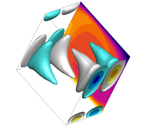
The three-dimensional perturbations arising from the linear stability analysis will later be visualized using the  $y$-component of vorticity,
  $\omega _y$. This component is convenient because it reveals the three-dimensional disturbance structures, while reverting to zero in the two-dimensional limit. Rotation about
  $z$ by
  $180^\circ$ changes the sign of
  $\omega _y = \partial _z u - \partial _x w$. This occurs as under this rotation, both
  $u$ and
  $\partial _x$ change sign. Hence disturbances may share centro-symmetry with the base flow, such that
 \begin{equation} \left.\begin{array}{c@{}} (u,v,w,T)({-}x,-y) = ({-}u,-v,w,-T)(x,y),\\[2pt] \text{therefore}\quad \omega_y({-}x,-y) ={-}\omega_y(x,y), \end{array}\right\} \end{equation}
or they may possess anti-centro-symmetry, i.e.
 \begin{equation} \left.\begin{array}{c@{}} (u,v,w,T)({-}x,-y) = (u,v,-w,T)(x,y),\\[2pt] \text{therefore}\quad \omega_y({-}x,-y) = \omega_y(x,y). \end{array}\right\} \end{equation}
Perturbations that satisfy neither of these constraints are simply referred to herein as being non-symmetric.
3. Results
3.1. Validation of two-dimensional flows at stably stratified inclinations ( $\theta \leq 90^\circ$)

Various authors have presented findings regarding the two-dimensional flows concerned in this study (Page Reference Page2011; Grayer et al. Reference Grayer, Yalim, Welfert and Lopez2020) or for three-dimensional experimental configurations representing a similar system (Inaba & Fukuda Reference Inaba and Fukuda1984; Corvaro, Paroncini & Sotte Reference Corvaro, Paroncini and Sotte2012; Jiang, Sun & Calzavarini Reference Jiang, Sun and Calzavarini2019). Thus §§ 3.1 and 3.2 do not intend to explore new findings with regard to the two-dimensional problem, but rather serve to provide a brief overview of the two-dimensional solutions, as well as to validate the computational methods against results presented in the literature.
Temperature contours of the steady two-dimensional base flows corresponding to  $R_{N}=1$,
  $10^{2}$ and
  $10^{4}$ are presented for
  $\theta =30^\circ$,
  $60^\circ$ and
  $90^\circ$ in figure 3. Equispaced isotherms almost parallel to the conducting walls are observed at low buoyancy numbers. Viscous and buoyancy forces are balanced when
  $R_{N}=1$, and the temperature differential between the conducting walls produces a constant temperature gradient throughout the fluid. Buoyancy forces become more significant as
  $R_{N}$ is increased, and the contributions from the nonlinear terms in the governing equations are no longer negligible. The flow becomes relatively faster as the buoyancy number is increased to
  $R_{N}=10^{2}$. Isotherms at the centre of the enclosure begin to bend towards the horizontal, and this bending becomes more apparent as
  $\theta$ increases as the isotherms must meet insulating walls at right angles to satisfy the adiabatic boundary condition. A tightening of isotherms is observed near the two opposing corners B and D, and separation of isotherms is evident at the other two opposing corners A and C. The tightening of the isotherms implies a higher required heat flux to maintain the fixed temperatures at the walls, and this temperature gradient induces a baroclinic torque that drives the circulation of the flow (Grayer et al. Reference Grayer, Yalim, Welfert and Lopez2020).

Figure 3. Temperature contours of the two-dimensional base flow shown with 14 equispaced isotherms for the indicated values of  $R_N$ and
  $\theta$. Light and dark shading represent hot and cold regions, respectively.
Streamlines are shown for inclinations  $\theta =60^\circ$ and
  $90^\circ$ at
  $R_{N}=10^{4}$ in figure 4. At this
  $R_N$, buoyancy forces take precedence over diffusive effects, and the flow is no longer a circulation about the centre of the enclosure. The fastest observed flows are now the near-wall flows along the conducting walls, with the cold, dense fluid travelling down the cold wall, and the hot, lighter fluid rising along the hot wall. For inclinations
  $\theta \leq 45^\circ$, these near-wall flows exit corners B and D, and travel along the adjacent conducting walls and a portion of the adiabatic walls before returning horizontally to the aforementioned corners. The central region is stratified, and separates two isothermal, triangular regions near corners A and C. These isothermal regions are similarly observed at inclinations
  $45^\circ < \theta <90^\circ$, but significant differences are present. The fluid travels along a partial length of the conducting walls before returning horizontally at relatively slower speeds and impinging on the corner region of the opposing conducting walls. The horizontal shear flows populate the central region of the enclosure, separating two isothermal regions.

Figure 4. Temperature contours overlaid with equispaced streamfunction contour lines for the flow at  $R_N=10^4$ at inclinations (a)
  $\theta =60^\circ$ and (b)
  $\theta =90^\circ$. Contour levels are as per figure 3.
Flow properties vary significantly at  $\theta = 90^{\circ }$, at which the configuration represents the extensively studied differentially heated square problem. The flow is now characterized by narrow boundary layers along almost the entirety of the conducting walls, and a stratification of the flow is evident in the centre region, bearing resemblance to that of the untilted configuration. This stratification is broken by two local recirculations in the opposing corners A and C, which develop due to the faster near-wall flows at the conducting walls encountering the insulating walls. The flow adjacent to these recirculations is observed to detach from the insulating walls.
The critical  $R_N$ corresponding to the onset of two-dimensional instability is predicted via linear stability analysis by evaluating the case where the spanwise wavenumber is set to
  $m=0$ (corresponding to a two-dimensional perturbation). Results for enclosure inclinations
  $60^\circ \leq \theta \leq 90^\circ$ are presented in figure 5, where they are compared to a subset of the data obtained by Grayer et al. (Reference Grayer, Yalim, Welfert and Lopez2020). Critical values of
  $R_N$ for inclinations below
  $\theta =60^\circ$ were not obtained in the present study due to the increasingly severe time step size restriction at the higher
  $R_N$ values.

Figure 5. Critical  $R_N$ corresponding to two-dimensional instability plotted against
  $\theta$. Results obtained in the current study (black) are compared against a subset of values from Grayer et al. (Reference Grayer, Yalim, Welfert and Lopez2020) (red). The three modes
  $L_{1}$,
  $L_{2}$ and
  $L_{3}$ and their corresponding domains are shown.
Bifurcation is identified to occur through three distinct modes for  $\theta \leq 90^\circ$; Grayer et al. (Reference Grayer, Yalim, Welfert and Lopez2020) denoted these as
  $L_{1}$,
  $L_{2}$ and
  $L_{3}$, respectively occurring for
  $60^\circ \leq \theta \leq 83^\circ$,
  $83^\circ \leq \theta \leq 88^\circ$ and
  $88^\circ \leq \theta \leq 90^\circ$. As a general trend, the critical
  $R_{N}$ is observed to decrease with increasing values of
  $\theta$, with the
  $L_{2}$ and
  $L_3$ transitions being exempt from this trend. The flow loses its stability to the
  $L_{1}$ mode due to the imbalance between the near-wall flows on the conducting and insulating walls, as horizontal shear flows in the central region of the enclosure perturb the near-wall flows at the conducting walls. Here,
  $L_{2}$ breaks the steady state as
  $\theta$ is increased beyond
  $83^\circ$. The horizontal shear layers are now mixed into their boundary layers of the insulating walls, and buoyancy forces contribute more effectively to the increase in flow velocity near the wall due to the increase in tilt angle. These fast near-wall flows strike the corners of the enclosure, and lead to the development of a localized instability. Mode
  $L_{3}$ occurs through mechanisms similar to those for
  $L_{2}$: the fast near-wall flows along the conducting walls drive into the corners, rebounding as they meet the insulating walls. This displaces the hotter/colder fluid at the top/bottom walls, which results in a convectively unstable region as the hotter, buoyant fluid is now beneath cooler regions (Gill Reference Gill1966; Ivey Reference Ivey1984; Paolucci & Chenoweth Reference Paolucci and Chenoweth1989; Grayer et al. Reference Grayer, Yalim, Welfert and Lopez2020).
Minimal differences are observed when comparing the neutral stability curve determined in the current study against published results of Grayer et al. (Reference Grayer, Yalim, Welfert and Lopez2020), providing quantitative validation of the computational methods employed in the current study.
3.2. Two-dimensional base flows at unstably stratified inclinations ($90^\circ < \theta \leq 180^\circ$)

Base flow solutions at lower inclinations are presented for  $R_N=10^4$ in the previous subsection. However, flows at inclinations above
  $\theta \approx 115^\circ$ become unsteady at
  $R_N \approx 10^4$. It is thus more reasonable to describe the flows at higher inclinations (
 $\theta >90^\circ$) in their steady state when comparing flow characteristics to lower inclinations (
 $\theta \leq 90^\circ$), rather than at the same
  $R_N$.
Temperature contours and overlaying streamlines for flows at higher inclinations ( $\theta >90^\circ$) are presented in figure 6 for
  $R_N$ just below the critical threshold where the flow becomes unsteady. At
  $R_N=10^4$ and
  $\theta =105^\circ$, the stratification of the central region is weaker than at
  $\theta =90^\circ$ for the same
  $R_N$, and the near-wall flows are relatively slower as the conducting walls are no longer parallel to the direction of gravity. This results in the disappearance of the recirculations in the enclosure corners identified at
  $\theta =90^\circ$, and the flow now detaches further along the insulating walls, with recirculations observed within and adjacent to the detached flow structure. The flow structure is predominantly a circulation about the centre of the enclosure at
  $\theta =135^\circ$ and
  $R_N=10^3$, with the fastest flow being observed in the boundary layers near the conducting walls. The circulation is significantly slower away from the enclosure walls, and the central region is defined by three weak recirculations and a low temperature gradient. The strength of these recirculations becomes negligible compared the rest of the flow for the same
  $R_N$ at
  $\theta =150^\circ$, and the temperature gradient in the central region is now significantly lower compared to smaller inclinations. The central region is isothermal when
  $R_N=10^3$ and
  $\theta =180^\circ$, where the enclosure represents the Rayleigh–Bénard configuration, and the flow is primarily a circulation about the centre of the enclosure; two secondary circulations similar to those described by Chandra & Verma (Reference Chandra and Verma2011) are observed in corners B and D.

Figure 6. Temperature contours overlaid with equispaced streamfunction contour lines for the flow at parameters of (a)  $R_N=10^4$,
  $\theta =105^\circ$, (b)
  $R_N=10^3$,
  $\theta =135^\circ$, (c)
  $R_N=10^3$,
  $\theta =150^\circ$, and (d)
  $R_N=10^3$,
  $\theta =180^\circ$. Contour levels are as per figure 3.
Exclusive to the  $\theta =180^\circ$ scenario, there is an isolated flow regime where an unsteady thermal plume structure develops at
  $R_N\approx 210$, and the steady state regains stability as the buoyancy number is increased beyond
  $R_N\approx 269$, with the flywheel structure taking precedence once again (figure 7). The thermal plume structure is defined by a rising plume of hotter fluid in the centre of the enclosure separating two circulations where cold fluid is sinking on both sides of the plume, with the circulation on the right being stronger than that on the left (figure 7b). This structure is similarly observed in Hier Majumder, Yuen & Vincent (Reference Hier Majumder, Yuen and Vincent2004) in what was referred to as the diffusive-viscous regime.

Figure 7. Temperature contours overlaid with equispaced streamfunction contour lines showing the progression of the base flow structure at  $\theta =180^\circ$ as
  $R_N$ is increased from
  $199.5$ to
  $269.2$. The steady flywheel structure is shown at (a)
  $R_N = 199.5$ and (c)
  $R_N=269.2$. (b) An instantaneous snapshot of the unsteady flow at
  $R_N=234.4$ depicting the thermal plume structure. Contour levels are as per figure 3.
3.3. Growth rate dependence on wavenumber
Prior studies on natural convection flows in square enclosures have applied linear stability analysis to investigate the stability of these flows with regard to both two- and three-dimensional perturbations, and found that the base flow is often more unstable to the latter (Henkes & Le Quéré Reference Henkes and Le Quéré1996; Xin & Le Quéré Reference Xin and Le Quéré2001; Dimopoulos & Pelekasis Reference Dimopoulos and Pelekasis2012), prompting the current study to focus on three-dimensional perturbations. This subsection evaluates the dependence of the perturbation growth rate on wavenumber  $m$, buoyancy number
  $R_{N}$ and inclination angle
  $\theta$. Positive growth rates are calculated from both real and complex conjugate eigenvalues, which respectively correspond to stationary and oscillatory instability modes (Ng et al. Reference Ng, Vo and Sheard2018; Mayeli et al. Reference Mayeli, Tsai and Sheard2022).
Growth rate is plotted against spanwise wavenumber for various inclinations in figure 8. The growth rate versus wavenumber profile reveals the development of two local maxima at enclosure inclinations  $58^\circ \leq \theta \leq 82^\circ$, as shown for
  $\theta =60^\circ$ in figure 8(a). The first local maximum consists of positive real multipliers occurring at lower wavenumbers (
 $m\leq 10$ for considered
  $R_{N}$), and the second maximum contains complex eigenvalues. Instability first emerges at this maximum, while the stationary mode remains stable at the critical
  $R_{N}$. This stationary mode also loses stability as
  $R_N$ is further increased, though there is no indication that it will become unstable beyond the oscillatory mode. The flow is more unstable to two-dimensional than three-dimensional perturbations for an exclusive range of inclinations
  $83^\circ \leq \theta \leq 87^\circ$ (figures 8b,c), with
  $m=0$ presenting growth rates that exceed the instability threshold at lower values of
  $R_{N}$ as compared to non-zero values of
  $m$. The onset of instability is predicted to occur through an oscillatory mode, and
  $\sigma$ decays with increasing values of
  $m$. The exception to this is at
  $\theta =87^\circ$, where a second local maximum comprising positive real multipliers develops near
  $30\leq m \leq 35$. This second local maximum remains below the stability threshold at the critical
  $R_{N}$ when the flow becomes unsteady to two-dimensional disturbances, but becomes unstable with a slight increase in
  $R_{N}$, though it does not demonstrate the potential to become unstable beyond the two-dimensional mode (figure 8c).

Figure 8. Growth rate  $\sigma$ plotted against wavenumber
  $m$ for various
  $R_N$ at inclinations (a)
  $60^\circ$, showing the development of two maxima with the oscillatory mode becoming unstable, (b)
  $85^\circ$, showing the two-dimensional mode becoming unstable, (c)
  $87^\circ$, showing the two-dimensional mode becoming unstable with a stationary three-dimensional mode emerging, and (d)
  $90^\circ$, showing the stationary mode becoming unstable. For all cases, the red symbols denote a real multiplier indicative of a stationary instability, and hollow black symbols denote complex multipliers that are indicative of an oscillatory instability.
At enclosure inclinations  $88^\circ \leq \theta < 180^\circ$, the primary instability modes are stationary. The relationship between growth rate and wavenumber is dominated by the emergence of two local maxima comprising real multipliers, with the second maximum (at higher values of
  $m$) crossing the stability threshold. The first maximum is subtle and does not demonstrate the potential to exceed the second maximum. For inclinations
  $88^\circ \leq \theta \leq 100^\circ$, the first local maximum is identified near
  $2 \leq m \leq 5$ and gradually shifts towards
  $m=0$ as
  $\theta$ increases, reaching
  $m=0$ at
  $\theta =105^\circ$ (figure 9a), then departing towards
  $2 \leq m \leq 5$ as the enclosure inclination is increased beyond
  $\theta \approx 158^\circ$ (figure 9c). A unique relationship between growth rate and wavenumber is presented for
  $\theta =180^\circ$. A substantial increase in peak growth rate is observed immediately after increasing
  $R_N$ beyond its critical value (figure 9d), as opposed to other inclinations where the peak growth rate gradually increases with increasing
  $R_N$. This single maximum is identified near
  $3.5 \leq m \leq 4.5$.

Figure 9. Growth rate  $\sigma$ plotted against wavenumber
  $m$ for various
  $R_N$ at inclinations (a)
  $105^\circ$, (b)
  $135^\circ$ and (c)
  $165^\circ$, showing the dual peak profile, with the first maximum remaining stable and shifting towards higher values of
  $m$ as
  $\theta$ increases, whilst the second maximum corresponding to a stationary mode becomes unstable. (d) The growth rate profile for
  $180^\circ$, revealing a sudden jump in peak growth rate as
  $R_N$ is pushed just above its critical value. Symbol shading is as per figure 8.
3.4. Neutral stability
Critical  $R_N$ is plotted against
  $\theta$ in the neutral stability map shown in figure 10(a). Three distinct regions can be identified, with the two-dimensional oscillatory branch separating the three three-dimensional oscillatory and five synchronous branches. The lowest enclosure inclination at which three-dimensional transition occurs (within the range of testable parameters) is predicted to be
  $\theta =58^\circ$, occurring at buoyancy number
  $R_N=2.54\times 10^4$. The neutral stability curve indicates that lower values of
  $\theta$ become unstable to three-dimensional disturbances as
  $R_N$ increases; three-dimensional linear stability analysis results for these parameters were not obtained as the time step restriction made computation impractical.

Figure 10. Variation of critical (a)  $R_N$ and (b)
  $m$ with enclosure inclination
  $\theta$. Solid black lines connect where the flow is predicted to become unstable to an oscillatory mode, whereas red dashed lines correspond to a stationary mode. Eight leading three-dimensional instability modes are identified along with one two-dimensional (2-D) mode, as labelled in (b).
The onset of instability is predicted to occur through an oscillatory mode for inclinations  $58^\circ \leq \theta \leq 87^\circ$, and the critical
  $R_N$ continually decreases from
  $2.54 \times 10^4$ to a local minimum
  $1.55 \times 10^4$ when
  $\theta$ is increased from
  $58^\circ$ to
  $71.4^\circ$. Critical
  $R_N$ then increases to a local maximum
  $R_N = 1.98 \times 10^4$ at inclination
  $\theta = 81^\circ$ before beginning to decrease with increasing angle once again.
The dominant instability mode switches from a three-dimensional oscillatory mode to the two-dimensional oscillatory mode for inclinations  $83^\circ \leq \theta \leq 87^\circ$. Although the flow is more unstable to two-dimensional disturbances across this range of enclosure inclinations, we note that even a marginal increase in
  $R_N$ past the critical value results in the three-dimensional mode becoming unstable. Critical
  $R_N$ decreases from
  $R_N = 1.86 \times 10^4$ at
  $\theta = 83^\circ$ to a local minimum
  $R_N = 1.31 \times 10^4$ at
  $\theta = 85.3^\circ$ before increasing to a maximum
  $R_N = 1.39 \times 10^4$ when
  $\theta = 87^\circ$. The primary instability mode is predicted to switch to a stationary mode beyond this enclosure inclination. This change in leading instability mode is accompanied by a steep decrease in critical buoyancy number to
  $R_N = 5.92\times 10^3$ at
  $\theta =88^\circ$, and then again to
  $R_N = 4.67 \times 10^3$ at
  $\theta = 90^\circ$. Critical
  $R_N$ is then observed to decrease monotonically to
  $R_N\approx 467.7$ as the enclosure inclination is increased to
  $\theta =142^\circ$. Subsequently, it increases to
  $R_N\approx 661$ at
  $\theta =157^\circ$, before finally decreasing once more to
  $R_N \approx 211$ at
  $\theta =180^\circ$.
Elucidation of the distinct instability modes across the neutral stability boundary can be revealed through discontinuities in the corresponding critical spanwise wavenumbers. Figure 10(b) shows the critical wavenumber plotted against  $\theta$. Nine different primary instability modes are identified, with eight being three-dimensional and one being two-dimensional. The first corresponds to inclinations
  $58^\circ \leq \theta \leq 64^\circ$, where
  $m_c$ is observed to decrease almost linearly from
  $45.4$ to
  $37.1$ with increasing
  $\theta$. The emergence of the second oscillatory mode is accompanied by an abrupt decrease in critical wavenumber to
  $m_c=33.1$ as the inclination is increased to
  $\theta =65^\circ$. Minimal variation in
  $m_c$ is exhibited for inclinations
  $65^\circ \leq \theta \leq 79^\circ$ that define this mode, where
  $m_c$ remains within
  $\pm$5 % of
  $m=31$. Further decrease in
  $m_c$ to
  $16.2$ signals a change to the third oscillatory, three-dimensional mode, which corresponds to inclinations
  $80^\circ \leq \theta \leq 82^\circ$, where
  $14.7 \leq m_c \leq 16.2$. For convenience, these modes will be referred to as mode 1, mode 2 and mode 3, corresponding to inclinations
  $58^\circ \leq \theta \leq 64^\circ$,
  $65^\circ \leq \theta \leq 79^\circ$ and
  $80^\circ \leq \theta \leq 82^\circ$, respectively. The frequencies of these instability modes are presented in table 2 for parameters near the critical stability threshold.
Table 2. Dimensionless frequencies of oscillatory three-dimensional instability modes at parameters near the critical stability threshold.

A steep decrease to  $m_c=0$ is then observed at inclinations
  $83^\circ \leq \theta \leq 87^\circ$, corresponding to the dominant mode switching to the two-dimensional mode. This two-dimensional mode separates the oscillatory and stationary branches, with all inclinations above
  $\theta =87^\circ$ becoming unstable to a stationary instability. The critical wavenumber increases to
  $m_c=21$ at
  $\theta =88^\circ$ with the emergence of the first stationary instability mode, which will be denoted mode 4. A sudden decrease to
  $m_c=5.9$ at
  $\theta =100^\circ$ is then observed with the introduction of the mode 5 instability, which is the dominant mode across inclinations
  $100^\circ \leq \theta \leq 116^\circ$, and
  $m_c$ remains within the range
  $5.9 \leq m_c \leq 7$. The critical wavenumber then increases to
  $m_c=12.1$ at
  $\theta =117^\circ$, corresponding to a new stationary instability (which will be denoted mode 6) emerging as the dominant mode. The mode 6 instability is predicted to be the primary instability mode across inclinations
  $117^\circ \leq \theta \leq 158^\circ$, and the critical wavenumber demonstrates slight variation, dropping to a minimum
  $m_c = 8.5$ at
  $\theta \approx 130^\circ$ before increasing to
  $m_c = 10.4$ at
  $\theta \approx 158^\circ$. The dominant instability mode switches to mode 7 at
  $\theta \approx 159^\circ$, but without a significant change in
  $m_c$ as compared to mode 6, and the main distinction between the two modes is in their different spatial structures (which will be elaborated on in the next subsection). Across this branch of instability, there is a gradual decrease in the critical wavenumber with an increase in inclination, from
  $m_c=10.4$ at
  $\theta \approx 159^\circ$, to
  $m_c=6.4$ at
  $\theta =179^\circ$. The final instability mode identified in this study is referred to as mode 8, and is exclusive to
  $\theta =180^\circ$. The emergence of this mode is accompanied by a sudden drop in the critical wavenumber to
  $m_c=4$, which is the lowest predicted non-zero value of
  $m_c$ across the considered range of enclosure inclinations.
Perturbation growth rate is plotted against spanwise wavenumber, with both the leading and first subdominant eigenvalues plotted at  $\theta =158^\circ$ when
  $R_N = 832$, in figure 11. It is apparent that at this combination of parameters, two distinct instability modes are unstable, with peak wavenumbers of approximately
  $m=12$ (leading eigenmode) and
  $m=13$ (first subdominant eigenmode). As the range of incidence angles is traversed, the dominant mode is repeatedly supplanted by other modes, leading to the array of modes identified in the neutral stability curve in figure 10(a). These neighbouring dominant modes in some cases have quite different wavenumbers, leading to the discontinuous nature of the data in figure 10(b).

Figure 11. Growth rate  $\sigma$ plotted against wavenumber
  $m$ for
  $\theta =158^\circ$ when
  $R_N = 832$, showing the modes corresponding to the leading (red) and first subdominant (blue) eigenmodes. Filled symbols denote a complex conjugate multiplier indicative of an oscillatory instability, and hollow symbols denote a real multiplier that is indicative of a stationary instability. Modes 6 and 7 are both identified, with mode 7 being the dominant instability mode.
3.5. Spatial structure of unstable modes
Iso-surfaces of the  $y$-component of vorticity (
 $\omega _y$) corresponding to the most unstable mode are obtained by superimposing the Fourier mode of the instability onto its corresponding two-dimensional base flow. A reminder that as per (2.13), centro-symmetry leads to opposite-signed
  $\omega _y$ values under
  $180^\circ$ rotation about
  $z$. Conversely, anti-centro-symmetry manifests as same-signed
  $\omega _y$ under the same rotation (2.14). Perturbation structures obtained at inclinations
  $\theta = 60^\circ$,
  $75^\circ$ and
  $82^\circ$, respectively corresponding to the oscillatory modes 1, 2 and 3, are presented in figure 12.

Figure 12. The temperature field of the two-dimensional base flow with three-dimensional perturbation structures representing the  $y$-component of vorticity (
 $\omega _y$) for the flow at (a)
  $\theta =60^\circ$,
  $R_N=2.15 \times 10^4$,
  $m=44$, (b)
  $\theta =75^\circ$,
  $R_N=1.67 \times 10^4$,
  $m=32$, and (c)
  $\theta =82^\circ$,
  $R_N=1.95 \times 10^4$,
  $m=16$. These correspond to modes 1, 2 and 3, respectively. Temperature contours are as per figure 3. White and blue iso-surfaces represent positive and negative values of
  $\omega _y$, respectively, and contour levels are arbitrarily selected to elucidate the structure of the mode. (d) A zoomed-in snapshot of the two-dimensional temperature field overlaid with streamfunction contour lines corresponding to where the perturbation structures develop near the cold wall in (b), showing the thermal boundary layer. The supplementary movie 1 available at https://doi.org/10.1017/jfm.2024.1210 animates the oscillatory modes 1, 2 and 3.
Perturbation structures corresponding to modes 1, 2 and 3 primarily develop adjacent to the boundary layers along the conducting walls at the vertical height of the opposing corners B and D, corresponding to regions where horizontal shear layers return to the central region from the thermal boundary layer (figure 12d). Significant differences are identified between the three instability modes despite their development in similar regions of the enclosure. Mode 1 dominates near the cold wall, whereas the instability develops adjacent to both hot and cold walls at similar intensities for modes 2 and 3. Modes 2 and 3 are similarly centro-symmetric about the centre of the enclosure, but mode 3 presents a significant difference in that the instability is also observed to develop along the insulating wall where the flow structure detaches from the wall.
As mentioned previously, flows at inclinations  $83^\circ \leq \theta \leq 87^\circ$ are more unstable to two-dimensional perturbations as compared to three-dimensional ones. An oscillatory instability develops primarily within the downstream region of the near-wall flows along the conducting walls (figure 13). Xin & Le Quéré (Reference Xin and Le Quéré2002) observed that flows in a differentially heated cavity with an 8 : 1 height to width aspect ratio are similarly more unstable to two-dimensional perturbations due to a boundary layer type instability.

Figure 13. Snapshot of the perturbation vorticity shown along with streamlines for the two-dimensional oscillatory mode at  $\theta =85^\circ$,
  $R_N=1.58\times 10^4$, showing the entire enclosure (left) and zoomed in snapshot of the perturbation structure (right).
The perturbation structures are shown for modes 4, 5 and 6 in figure 14. The mode 4 structure is anti-centro-symmetric and dominates in corners A and C, corresponding to the location of the local recirculations. The structures extend towards the centre of the insulating wall and follow the curvature of where the base flow detaches from the insulating wall. Mode 5 structures are similarly anti-centro-symmetric but present distinct differences. The instability is now observed to develop predominantly at positions aligning with the recirculations in the central region of the enclosure, as well as at multiple points along the insulating wall, i.e. at the centre and adjacent to the ends where it meets the flow near the conducting walls. Mode 6 perturbation structures are centro-symmetric and are observed separately at both ends of the insulating walls, being stronger at the end where the flow along the conducting walls impinges onto the insulating wall. The instability also develops adjacent to the thermal boundary layers along the conducting walls, with its intensity decaying as it progresses in the direction opposite to the flow. The features of the mode 6 structures change drastically with increasing inclination as the instability near the conducting wall develops less along the  $x$-direction and instead extends towards the
  $y$-direction (relative to lower inclinations). This is highlighted in figure 15(a), where perturbation structures corresponding to mode 6 at higher inclinations (as compared to those presented in figure 14), mode 7 and mode 8 are displayed.

Figure 14. Perturbation structures of  $\omega _y$ shown for the flow at (a)
  $\theta =90^\circ$,
  $R_N=4.67 \times 10^3$,
  $m=20$, (b)
  $\theta =105^\circ$,
  $R_N=1.99 \times 10^3$,
  $m=6$, and (c)
  $\theta =120^\circ$,
  $R_N=10^3$,
  $m=12$. These correspond to modes 4, 5 and 6, respectively. Iso-surfaces and contours are as per figure 12.

Figure 15. Perturbation structures of  $\omega _y$ shown for the flow at (a)
  $\theta =150^\circ$,
  $R_N=630.9$,
  $m=10$, (b)
  $\theta =165^\circ$,
  $R_N=562.3$,
  $m=9$, (c)
  $\theta =180^\circ$,
  $R_N=251.2$,
  $m=4$. These correspond to modes 6, 7 and 8, respectively. Iso-surfaces and contours are as per figure 12.
Mode 7 is characterized by anti-centro-symmetric structures that develop primarily along the insulating walls, with its intensity peaking near corners B and D; perturbation structures are also observed in the central region at locations corresponding to the edge of the isothermal region.
The structures of the base flows that lose their stability to modes 4, 5, 6 and 7 allude to a centrifugal instability, with a strong rotation about the centre of the enclosure. The stationary nature of these modes, their (anti-)centro-symmetric perturbation structures, and the concave boundary layers further suggest a Taylor–Görtler instability. This is observed similarly in Xin & Le Quéré (Reference Xin and Le Quéré2001) for a differentially heated cavity flow, and Ramanan & Homsy (Reference Ramanan and Homsy1994) for a lid-driven cavity flow. The perturbation structure corresponding to mode 8 is displayed in figure 15(c) and develops exclusively for  $\theta =180^\circ$. The perturbation structures are observed to form along the insulating walls and at points almost outlining the thermal plume structure. Unlike all other identified modes, the instability does not demonstrate any form of centro-symmetry, and is instead anti-symmetric about
  $x=0$ and
  $z=\lambda /2L$.
3.6. Nonlinear analysis of the three-dimensional transition
Three-dimensional DNS are performed to model the nonlinear dynamics of the transition as well as validate the linear stability analysis predictions. The current three-dimensional algorithm takes advantage of the assumed homogeneity of the geometry, and applies a Fourier spectral method in the out-of-plane  $z$-direction alongside the two-dimensional spectral element discretization in the
  $x$–
$x$– $y$ plane (Ryan, Butler & Sheard Reference Ryan, Butler and Sheard2012; Sapardi et al. Reference Sapardi, Hussam, Pothérat and Sheard2017). Resolution studies concluded that 8 Fourier modes sufficiently resolved the flow to within 0.1 % relative error relative to 32 Fourier modes, with regard to the out-of-plane spanwise velocity
  $w$ measured at a local point.
Three-dimensional simulations were performed for various enclosure inclinations at  $R_N$ just above the critical value to provide coverage of all identified instability modes. The out-of-plane spanwise domain length was set to match the wavelength of corresponding leading instability modes for each scenario. The flow is periodic in the spanwise direction, and is initialized with small random three-dimensional perturbations superimposed on the two-dimensional base flow solution.
The time history of the spanwise velocity  $w$ measured at a local point is displayed in figure 16(a) for
  $\theta =75^\circ$,
  $R_N=1.778\times 10^4$,
  $m=32$, and in figure 16(b) for
  $\theta =90^\circ$,
  $R_N=5.012\times 10^3$,
  $m=20$. The oscillatory and stationary behaviour of
  $w$ presented respectively in figures 16(a,b) is in good agreement with the eigenmodes predicted from the linear stability analysis for the same parameters.

Figure 16. Time histories of  $w$-velocity measured at a local point for (a)
  $R_N=1.78\times 10^4$,
  $\theta =75^\circ$,
  $m=32$, and (b)
  $R_N=5.01\times 10^3$,
  $\theta =90^\circ$,
  $m=20$, respectively showing the oscillatory and stationary nature of the instability.
The perturbation growth rate can be calculated from the time history of  $w$ at small amplitudes, and comparisons between growth rates calculated from the linear stability analysis and DNS are presented in table 3 for five different cases, each representing a different instability mode. The linear stability analysis predictions align closely with the DNS results, with the percentage difference being below 1 % for all considered cases.
Table 3. Comparison between growth rates predicted from the linear stability analysis (LSA) against three-dimensional DNS.

Vorticity perturbation structures predicted by the linear stability analysis are compared against the actual three-dimensional state produced once the flow saturates in figure 17 for modes 4 and 6. Perturbation structures obtained by the linear stability analysis closely mirror those obtained from the three-dimensional DNS for both mode 4 and mode 6. The symmetries and regions where the instabilities develop are consistent across the linear stability predictions and the DNS results. Small differences are observed in the mode 6 structures, with the DNS perturbation structures extending slightly further along both the  $x$- and
  $y$-axes. The symmetries of the modes produced by DNS are consistent with the predictions of the linear stability analysis for all identified three-dimensional modes, as demonstrated by the results presented in table 4. This, alongside the results for
  $\sigma$ presented in table 3, confirms that the linear stability analysis offers valuable predictions regarding the three-dimensional characteristics of the flow.

Figure 17. Visualization of the three-dimensional perturbation structures of the  $y$-component of vorticity for (a,b)
  $\theta =90^\circ$,
  $R_N=5.012 \times 10^3$,
  $m=20$, and (c,d)
  $\theta =120^\circ$,
  $R_N=954.9$,
  $m=12$. The leading eigenmode predicted by the linear stability analysis is presented in (a) and (c), and the saturated state of the corresponding three-dimensional DNS solution is shown in (b) and (d). Iso-surfaces and contours are as per figure 12.
Table 4. Comparison of symmetries in the leading three-dimensional modes derived from linear stability analysis (LSA) and those obtained from three-dimensional DNS for the specified parameters.

To understand the nature of the three-dimensional transition, a weakly nonlinear approximation can be applied to the flow. The flow is modelled as a complex oscillator, and the Stuart–Landau equation is employed to describe the growth and saturation of perturbation, and can be written as
 \begin{equation} \frac{\mathrm{d}A}{\mathrm{d} t}=(\sigma_{SL}+\mathrm{i}\omega)A-l(1+\mathrm{i}c)\,|A|^2\,A+\cdots, \end{equation}
where  $A = |A|\exp (\mathrm {i}\phi t)$ is the complex amplitude of a given signal (Landau & Lifshitz Reference Landau and Lifshitz1976). Equation (3.1) can then be decomposed into real and imaginary components as follows:
 $$\begin{gather} \frac{\mathrm{d} \log |A|}{\mathrm{d} t}=\sigma_{SL} - l\,|A|^2+\cdots, \end{gather}$$
 $$\begin{gather}\frac{\mathrm{d}\phi}{\mathrm{d} t}=\omega-lc\,|A|^2+\cdots, \end{gather}$$
where  $|A|$ and
  $\phi$ are the magnitude and phase angle of the signal, respectively,
  $\sigma _{SL}$ and
  $\omega$ respectively denote the growth rate and angular frequency, and coefficients
  $l$ and
  $c$ describe the nonlinear departure of the mode evolution from the linear regime. Considering up to second order of the real component described in (3.2a), the
  $l$ coefficient is of interest as it is a sufficient indicator of the nature of the bifurcation of the flow. The bifurcation is supercritical when
  $l>0$, whereas it is subcritical when
  $l<0$. This model has seen extensive application in various flow simulations, such as flows past cylindrical (Dušek, Le Gal & Fraunié Reference Dušek, Le Gal and Fraunié1994) and triangular (Ng et al. Reference Ng, Vo and Sheard2018) bluff bodies, flows in a differential-disk rotating system (Vo et al. Reference Vo, Montabone, Read and Sheard2015), and flows in confined channels (Sapardi et al. Reference Sapardi, Hussam, Pothérat and Sheard2017; Murali et al. Reference Murali, Ng and Sheard2022).
For the present study, an amplitude measure is taken as the square root of the integral of  $w$ over the computational domain, i.e.
 \begin{equation} A(t)^2=\langle w^2\rangle=\int_{\mathscr{V}}w^2\,\mathrm{d}\mathscr{V}, \end{equation}
where  $\mathcal {V}$ denotes the fluid volume. The analysis is carried out at various inclinations to capture the nonlinear bifurcation behaviour of each identified instability mode, with
  $R_N$ being chosen within 10 % of the critical
  $R_N$ for these simulations. Following the form of (3.2a), the time derivative of the amplitude logarithm is plotted against the square of the amplitude in figure 18(a) for
  $\theta =75^\circ$,
  $R_N=1.78\times 10^4$,
  $m=32$ growing from an oscillatory mode, and in figure 18(b) for
  $\theta =90^\circ$,
  $R_N=5.01\times 10^3$,
  $m=20$, which grows from a stationary mode. The positive gradient towards small values of
  $|A|^2$ in figure 18(a) indicates that the transition occurs through a subcritical bifurcation, whereas the near linear variation with a negative gradient throughout the entirety of figure 18(b) indicates transition through a supercritical bifurcation. The nature of transition to three-dimensionality does not demonstrate a dependence on whether the instability is oscillatory or stationary. This is demonstrated in figure 19, where the Landau coefficient is positive and negative for the oscillatory and stationary modes at
  $\theta =82^\circ$ and
  $120^\circ$, respectively, showing an opposite correlation to what was presented in figure 18. The nature of transition is evaluated for parameters that correspond to each different instability mode, and results are presented in table 5. For the considered parameters, modes 1, 2, 6 and 7 transition through a subcritical bifurcation, whereas modes 3, 4, 5 and 8 transition through a supercritical bifurcation.

Figure 18. Plots of  $\textrm {d}\log |A|/\mathrm {d} t$ against
  $|A|^2$, showing (a) a subcritical bifurcation, and (b) a supercritical bifurcation, of the two-dimensional flow to a three-dimensional state. The cases in (a) and (b) respectively represent parameters
  $\theta =75^\circ$,
  $R_N=1.78\times 10^4$,
  $m=32$ and
  $\theta =90^\circ$,
  $R_N=5.01\times 10^3$,
  $m=20$.

Figure 19. Plots of  $\textrm {d}\log |A|/\mathrm {d} t$ against
  $|A|^2$, showing (a) a supercritical bifurcation, and (b) a subcritical bifurcation, of the two-dimensional flow to a three-dimensional state. The cases in (a) and (b) respectively represent parameters
  $\theta =82^\circ$,
  $R_N=2.24\times 10^4$,
  $m=16$ and
  $\theta =120^\circ$,
  $R_N=954.9$,
  $m=12$.
Table 5. Characterization of bifurcations determined by Stuart–Landau analysis for three-dimensional instability modes predicted by linear stability analysis at the indicated parameters. Results suggest that the nature of transition to three-dimensionality has no correlation to the temporal nature of the eigenmodes.

Interestingly, it is observed that the DNS solution for mode 6 grows exponentially until reaching a stationary state (as predicted by the linear stability analysis), but then transitions to a fully chaotic state after a longer duration of time integration. This is demonstrated in figure 20, where  $\langle w^2 \rangle$ and
  $\log _{10} \langle w^2 \rangle$ are plotted against time. Under the Stuart–Landau model and as per Provansal, Mathis & Boyer (Reference Provansal, Mathis and Boyer1987), the amplitude of the instability is expected to be proportional to
  $(R_N-R_{N,c})^{1/2}$, where
  $R_{N,c}$ denotes the critical buoyancy number. In order to further characterize this transition to a fully chaotic state, we evaluate the variation of the linear instability mode growth rate and DNS instability amplitude (taking the domain integral of
  $w^2$ as the amplitude measure) with a parameter
  $\varepsilon$, which quantifies the distance between the buoyancy number and its corresponding critical buoyancy number:
  $\varepsilon =(R_N-R_{N,c})/R_{N,c}$. We observe a near-linear variation of
  $\langle w^2 \rangle$ with
  $\varepsilon$ for mode 1 in figure 21(c), which aligns with the proportionality law presented in Provansal et al. (Reference Provansal, Mathis and Boyer1987), and accurately reflects the minimal nonlinear effects observed in figure 17(b). Figure 21(d) presents a significantly different behaviour, whereby
  $\langle w^2 \rangle$ holds a value of zero at
  $\varepsilon =0$, then abruptly jumps to
  $\langle w^2 \rangle \approx 3.9\times 10^{-4}$ at
  $\varepsilon \approx 0.023$, after which the stationary solution stagnates and remains nearly constant as
  $\varepsilon$ continues to increase. The lack of a monotonic departure of the amplitude from zero as the control parameter is increased beyond its critical value is consistent with the behaviour of a subcritical bifurcation. Evidence of transition to a chaotic state is observed when
  $\varepsilon$ is increased past
  $\varepsilon \approx 0.023$, and the time-averaged
  $\langle w^2 \rangle$ branches off to values below those corresponding to the stationary state. This indicates that the saturated three-dimensional state is itself unstable, leading to the emergence of the chaotic behaviour. The transition to a chaotic state and the sudden increase in the stationary value of the amplitude measure are both expected to occur at values of
  $\varepsilon$ below what is shown in figure 21(d), but converged solutions at these values could not be obtained due to the increasingly exhaustive length of time integration closer to the instability threshold (where linear growth approaches zero).

Figure 20. Plots of (a)  $\langle w^2 \rangle$ and (b)
  $\log _{10} \langle w^2 \rangle$ against time for DNS solutions computed at
  $\theta =120^\circ$,
  $R_N=977.2$ and
  $m=12$, corresponding to mode 6. The instability is observed to grow exponentially until it reaches a stationary state, before evolving into a chaotic state.

Figure 21. Growth rate  $\sigma$ determined by linear stability analysis plotted against
  $\varepsilon$ for (a) mode 1 and (b) mode 6, and
  $\langle w^2 \rangle$ obtained from DNS plotted against
  $\varepsilon$ for (c) mode 1 and (d) mode 6. The solid red line in (d) represents the amplitude measure in the stationary state, and the black dashed line denotes the time-averaged amplitude after transitioning to a chaotic state. The red and black arrows in (d) assist in visualizing the abrupt increase in
  $\langle w^2 \rangle$ from zero to its value in the stationary state, and the decrease from its value in the stationary state to the time-averaged value in the chaotic state, respectively.
4. Conclusion
This paper reports on the stability of natural convection flows within a differentially heated square enclosure oriented at various inclinations to the horizontal. Results from the linear stability analysis indicate that the flow is first unstable to three-dimensional perturbations for the majority of considered inclinations in  $58^\circ \leq \theta \leq 180^\circ$, with the exception being enclosure inclinations
  $83^\circ \leq \theta \leq 87^\circ$ that are more unstable to two-dimensional perturbations.
The critical  $R_N$ corresponding to three-dimensional instability is observed to decrease non-monotonically with increasing inclination from
  $R_N=2.54 \times 10^4$ at
  $\theta =58^\circ$ to
  $R_N=213.8$ at
  $\theta =180^\circ$. This transition to three-dimensionality is predicted to occur through eight different instability modes, with each being dominant across a different range of inclinations. Modes 1, 2 and 3 are oscillatory, and are the primary modes for which the flow transitions for enclosure inclinations
  $58^\circ \leq \theta \leq 64^\circ$,
  $65^\circ \leq \theta \leq 79^\circ$ and
  $80^\circ \leq \theta \leq 82^\circ$, respectively, and develop predominantly where the flow returns horizontally from the near-wall flow. Enclosure inclinations
  $83^\circ \leq \theta \leq 87^\circ$ are most unstable to an oscillatory two-dimensional mode that dominates within the downstream region of the near-wall flows along the conducting walls. A similar feature was observed by Xin & Le Quéré (Reference Xin and Le Quéré2002) for a differentially heated cavity of large height to width aspect ratio. Flows at enclosure inclinations
  $88^\circ \leq \theta \leq 180^\circ$ lose their stability to stationary instability modes, with five different primary modes identified across this range of inclinations. Modes 4, 5, 6, 7 and 8 respectively correspond to enclosure inclinations
  $88^\circ \leq \theta \leq 99^\circ$,
  $100^\circ \leq \theta \leq 116^\circ$,
  $117^\circ \leq \theta \leq 158^\circ$,
  $159^\circ \leq \theta \leq 179^\circ$ and
  $\theta =180^\circ$. The symmetry and structural features of modes 4, 5, 6 and 7 suggest a Taylor–Görtler instability due to centrifugal forces, agreeing with the proposition made by Xin & Le Quéré (Reference Xin and Le Quéré2001) for a differentially heated cavity flow.
Three-dimensional DNS and the Stuart–Landau equation were applied to evaluate the nonlinear evolution of primary instability modes. Results indicate that transition from two-dimensional flow to three-dimensionality occur through either subcritical or supercritical bifurcation, with no correlation to the temporal nature of the eigenmodes.
The present study concerns two-dimensional flows in an enclosure containing a fluid characterized by a constant Prandtl number  $Pr=0.71$, and represents only scenarios corresponding to air at room temperature. It is therefore important to examine the effects of varying the Prandtl number to reflect a wider variety of fluids, as well as to extend the coverage of this problem to consider different aspect ratios to better reflect on the multitude of possible geometries present in the physical world, especially as prior studies have demonstrated the dependency of instability mechanisms on these parameters (Le Quéré & Alziary de Roquefort Reference Le Quéré and Alziary de Roquefort1985; Xin & Le Quéré Reference Xin and Le Quéré2001, Reference Xin and Le Quéré2006) for similar configurations. Additionally, the current study evaluates two-dimensional flows, where the three-dimensional instability mechanisms are predicated on the spanwise component extending infinitely in a homogeneous manner. Three-dimensional flows should be studied to evaluate the influence of the walls bounding the spanwise extent of the enclosure, and effects associated with the transverse flow movement.
Supplementary material
A supplementary movie is available at https://doi.org/10.1017/jfm.2024.1210.
Acknowledgements
The authors are grateful to H. Grayer II for his valuable communication and for laying the groundwork for the current study through his work. The authors would also like to thank K.R. Maryada for discussions regarding the various instability mechanisms present in heated square enclosures. H.K.S. received support from the Australian Government Research Training Programme. This research was supported by the Australian Government via the computational resources of the National Computational Infrastructure (NCI), and by Monash University, including the high-performance compute resources of the Monash e-Research Centre.
Declaration of interests
The authors report no conflict of interest.


