


1 Introduction
The development of aircraft transportation has brought an increase of air traffic volume and consequently an increasing number of issues related to environmental aspects, such as emissions of carbon and oxides of nitrogen and noise pollution. The jet exhaust from the aircraft engines results in pollutant discharge and is one of the main sources of environmental/community and interior noise. Current high-bypass-ratio turbofan engines have partially achieved good efficiency in terms of fuel consumption, pollution and noise emissions. Pollutant discharge as well as fuel consumption have been significantly lowered by decreasing the jet velocities exhausting from the engine, such a solution also being a benefit in terms of noise emissions. In order to keep the same thrust, an increase of the mass flow has to be adopted to compensate the jet velocity reduction. Ultra-high-bypass-ratio turbofan engine concepts provide a valid solution featuring a reduction of the jet velocity and an increase of the fan/nacelle diameter. The constraint in terms of ground clearance will lead to a close-coupled architecture for engine installation under the wing. A strong jet–wing interaction is therefore expected, giving rise to a significant increase of the radiated noise (Huber et al. Reference Huber, Omais, Vuillemin and Davy2009, Reference Huber, Drochon, Pintado-Peno, Cléro and Bodard2014) and to stronger flow–structure interactions. Indeed, pressure fluctuations generated by the exhausting jets may impinge on the fuselage, causing panel stress and vibrations. The stronger jet footprint on the fuselage could give rise to higher levels of interior noise in the cockpit and enhanced vibration noise re-emitted in the aeroacoustic field, as well as graver conditions for the structural strength of the panels.
Despite its importance in the design process of new aircraft configurations, few studies have been devoted to the subject, and this represents the main motivation of the present work.
As regards the installation effects, several works in the literature have focused attention on the shielding/scattering effect of an airframe surface on the far-field noise (see, among many others, the papers of Papamoschou & Mayoral (Reference Papamoschou and Mayoral2009) and Brown (Reference Brown2013)). Installation effects were also studied by Podboy (Reference Podboy2012), who exploited the beamforming technique to provide noise source localization maps addressing the effect of the surface geometry as well as the impact of different nozzle operating conditions. The shielding/scattering effect of a flat plate installed tangentially to a compressible jet was investigated in depth by Cavalieri et al. (Reference Cavalieri, Jordan, Wolf and Gervais2014), who derived a prediction model for far-field noise in installed configurations based on a wavepacket source educed from the free-jet case. The effect of the sweep angle of the trailing edge was further addressed in a more recent paper (Piantanida et al. Reference Piantanida, Jaunet, Huber, Wolf, Jordan and Cavalieri2015). The issue of the installation effects of a flat surface on the aerodynamic field was investigated by Brown & Wernet (Reference Brown and Wernet2014), who performed particle image velocimetry measurements for different lengths of the surface. The experimental database was exploited by the authors to lay the foundations for far-field noise prediction tools relying on computational fluid dynamics and computational aeroacoustics.
Nevertheless, a clear understanding of the driving parameters of the jet–surface interaction is still far from being reached. Piantanida et al. (Reference Piantanida, Jaunet, Huber, Wolf, Jordan and Cavalieri2015) outlined that, for jet–surface radial distances of the order of the nozzle diameter, a strong deformation of the aerodynamic field induced by the presence of the surface is expected. As pointed out by Di Marco et al. (Reference Di Marco, Camussi, Bernardini and Pirozzoli2013), knowledge of the wall pressure statistics is the basis to derive reliable prediction models for acoustic emissions aiming at the development of noise control tools. Far-field noise can be predicted by Amiet’s model giving as input the measured wall pressure spectrum (Amiet Reference Amiet1975, Reference Amiet1976). Such an approach was adopted by Lawrence, Azarpeyvand & Self (Reference Lawrence, Azarpeyvand and Self2011) to assess that the far-field noise in installed configurations is essentially driven by the scattering dipole source from the trailing edge. The necessity to investigate the incident pressure field on the surface together with the scattered one was clearly addressed by Vera et al. (Reference Vera, Lawrence, Self and Kingan2015).
The discussion above motivated the authors to carry out a parametric analysis of the jet–surface interaction phenomenon in terms of wall pressure statistics. The installation effects of a flat plate placed tangentially to an incompressible jet for different radial distances of the surface from the nozzle axis was the topic of a previous work by the same authors (see Di Marco, Mancinelli & Camussi Reference Di Marco, Mancinelli and Camussi2015). The wall pressure statistics as well as the spectral content were characterized in both the streamwise and spanwise directions, and succeeded to derive a scaling criterion for pressure autospectra. The coherence functions were also computed and foundations for wall pressure modelling were laid by the application of Corcos’ model (Corcos Reference Corcos1963; Farabee & Casarella Reference Farabee and Casarella1991).
The analysis is extended in the present work, where the results of further experiments involving simultaneous velocity and wall pressure measurements are presented. Velocity measurements were performed by a hot-wire anemometer moved along the direction normal to the flat plate for different axial positions in order to characterize the surface effect on the velocity field statistics. A streamwise microphone array was used to provide the axial evolution of the wall pressure fluctuation field. Cross-statistical analysis of the velocity and wall pressure fields is provided as well in the time and frequency domains. Flow structures induced by the jet–surface interaction and linked to the velocity and wall pressure fields are educed by the application of a conditional averaging procedure based on the wavelet transform of the velocity and pressure signals. The effects of the jet–plate distance as well as of the streamwise location and crosswise position in the direction orthogonal to the surface are explicitly addressed.
With respect to the real industrial problem of an engine jet interacting with an airframe component, the study carried out certainly presents some limitations. Specifically, the compressibility effects on the jet–surface interaction phenomenon as well as the presence of a background flight stream velocity are neglected in order to further simplify the analysis. The infinite flat plate also represents a simplified geometry (e.g. trailing-edge and high-lift device effects are not taken into account). Nevertheless, due to the novelty of the approach, this experimental investigation offers a basis for physical understanding and theoretical modelling of the jet–surface interaction. Indeed, Di Marco et al. (Reference Di Marco, Camussi, Bernardini and Pirozzoli2013) observed that the wall pressure statistics in supersonic turbulent boundary layers (TBLs) exhibits a behaviour very similar to that detected in incompressible flow conditions. The spectral and statistical features of wall pressure fluctuations were found to be not significantly affected by variation in Mach and Reynolds numbers. Such an outcome suggests that the results obtained in the present test case could probably be extended to configurations with higher jet velocities. Furthermore, the analysis of the jet–surface interaction in a static case is essential to subsequently quantify the impact of a flight velocity on the installation effects.
In agreement with the results presented in Di Marco et al. (Reference Di Marco, Mancinelli and Camussi2015), the mutual distance between the jet and the flat plate represents the key parameter in the physics of jet–surface interaction. The jet impingement and the downstream flow development over the plate are strongly dependent on such geometrical length scale. According to Picard & Delville (Reference Picard and Delville2000), the coupled investigation of velocity and pressure fluctuations helps to lay the foundations for modelling strategies of the turbulent jet flow. Indeed, the analysis of combined velocity and wall pressure measurements in the present test case permits a causality relation between velocity and wall pressure signals to be established through the characterization of multivariate statistics as well as the identification of the in-flow velocity structures associated with energetic wall pressure events. The resulting outcome can provide a deeper knowledge of the mechanisms underlying the jet–surface interaction phenomenon aiming for the development of noise control devices.
The paper is organized as follows. In § 2 a description of the experimental set-up is provided, whereas § 3 is devoted to the description of the conditioning procedure based on wavelet transform. The results concerning the characterization of the jet–surface interaction are presented in § 4, and the final remarks are addressed in § 5.
2 Experimental set-up and instrumentation
The experiments were performed in the Aerodynamics and Thermo-Fluid Dynamics Laboratory of the Department of Engineering at University Roma Tre. An incompressible jet facility reproducing the apparatus described in Chatellier & Fitzpatrick (Reference Chatellier and Fitzpatrick2005) was used. It is constituted by a centrifugal blower for the air flow generation, and a wide-angle diffuser that guides the inflow into a plenum chamber where honeycomb panels and turbulence grids are installed. The flow finally issues into a quiescent ambient through a convergent nozzle, whose diameter
 $D$
is 52 mm. A flat plate is installed parallel to the nozzle axis by a rigid traverse system. The experimental tests were carried out with the flat plate placed at different radial distances
$D$
is 52 mm. A flat plate is installed parallel to the nozzle axis by a rigid traverse system. The experimental tests were carried out with the flat plate placed at different radial distances
 $H$
from the nozzle axis, spanning the range
$H$
from the nozzle axis, spanning the range
 $1D$
–
$1D$
–
 $2.5D$
with a step of
$2.5D$
with a step of
 $0.5D$
. A sketch of the experimental set-up is shown in figure 1 (for a more detailed description of the set-up and for the characterization of the jet facility, the reader can refer to Di Marco et al.
Reference Di Marco, Mancinelli and Camussi2015).
$0.5D$
. A sketch of the experimental set-up is shown in figure 1 (for a more detailed description of the set-up and for the characterization of the jet facility, the reader can refer to Di Marco et al.
Reference Di Marco, Mancinelli and Camussi2015).

Figure 1. Sketch of the jet–plate experimental set-up.

Figure 2. Sketch of the instrumentation set-up;
 $\unicode[STIX]{x1D6FC}$
is the jet spreading angle.
$\unicode[STIX]{x1D6FC}$
is the jet spreading angle.
Table 1. Summary of the experimental configurations for the four flat-plate radial distances
 $H/D=1$
, 1.5, 2 and 2.5 (MIC
$H/D=1$
, 1.5, 2 and 2.5 (MIC
 $=$
microphone; HW
$=$
microphone; HW
 $=$
hot wire).
$=$
hot wire).
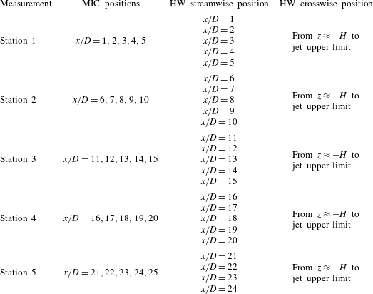
Simultaneous velocity and wall pressure measurements were carried out on the flow field generated by the interaction between the jet and the flat plate. The area of interest was divided into five measurement ‘stations’, each station being identified by five axial positions
 $x$
. A five-microphone array was placed at each station while a hot-wire probe was moved for each axial distance along the
$x$
. A five-microphone array was placed at each station while a hot-wire probe was moved for each axial distance along the
 $z$
-direction, i.e. the direction orthogonal to the flat plate. The movement of the probe in the
$z$
-direction, i.e. the direction orthogonal to the flat plate. The movement of the probe in the
 $z$
-direction was performed by a precision rail traversing system, which allowed us to reach a minimum distance between the hot wire and the surface of
$z$
-direction was performed by a precision rail traversing system, which allowed us to reach a minimum distance between the hot wire and the surface of
 $\unicode[STIX]{x1D701}=5$
mm. A representation of the instrumentation set-up as well as of the reference system adopted is shown in figure 2. A summary of the experimental configurations is reported in table 1.
$\unicode[STIX]{x1D701}=5$
mm. A representation of the instrumentation set-up as well as of the reference system adopted is shown in figure 2. A summary of the experimental configurations is reported in table 1.
Velocity signals were obtained using a single-component hot-wire (HW) probe (Dantec 55P11) of 1 mm length and
 $0.5~\unicode[STIX]{x03BC}\text{m}$
diameter connected to an anemometer (Constant Temperature Anemometer AN1003 Lab-System). Wall pressure signals were measured by electret microphones (Microtech Gefell M360), whose frequency response is flat in the range 20 Hz–20 kHz and whose full-scale value is 138 dB. Microphones were cavity-mounted and the pinhole was properly designed in order to move the Helmholtz resonant peak out of the measured frequency range. Data were acquired by a digital scope (Yokogawa DL708E) for an acquisition time
$0.5~\unicode[STIX]{x03BC}\text{m}$
diameter connected to an anemometer (Constant Temperature Anemometer AN1003 Lab-System). Wall pressure signals were measured by electret microphones (Microtech Gefell M360), whose frequency response is flat in the range 20 Hz–20 kHz and whose full-scale value is 138 dB. Microphones were cavity-mounted and the pinhole was properly designed in order to move the Helmholtz resonant peak out of the measured frequency range. Data were acquired by a digital scope (Yokogawa DL708E) for an acquisition time
 $T_{A}=20$
s at a sampling frequency
$T_{A}=20$
s at a sampling frequency
 $f_{s}=50$
kHz.
$f_{s}=50$
kHz.
The experiments were carried out at a jet velocity
 $U_{j}=42~\text{m}~\text{s}^{-1}$
, which corresponds to a Mach number
$U_{j}=42~\text{m}~\text{s}^{-1}$
, which corresponds to a Mach number
 $M_{j}\approx 0.12$
and a nozzle diameter-based Reynolds number
$M_{j}\approx 0.12$
and a nozzle diameter-based Reynolds number
 $Re_{D}\approx 1.5\times 10^{5}$
, which classifies the jet as a moderate-Reynolds-number jet (Bogey, Marsden & Bailly Reference Bogey, Marsden and Bailly2012).
$Re_{D}\approx 1.5\times 10^{5}$
, which classifies the jet as a moderate-Reynolds-number jet (Bogey, Marsden & Bailly Reference Bogey, Marsden and Bailly2012).
3 Conditional statistics analysis
The eduction of the flow structures underlying the jet–surface interaction phenomenon was achieved by the application of a wavelet conditioning procedure based on the detection of energetic events. The main concepts of the procedure are discussed in Camussi & Guj (Reference Camussi and Guj1999) and Camussi et al. (Reference Camussi, Grilliat, Caputi Gennaro and Jacob2010), whereas, for a comprehensive review on wavelet transform and its application, the reader may refer to Mallat (Reference Mallat1989), Daubechies (Reference Daubechies1992), Farge (Reference Farge1992) and Torrence & Compo (Reference Torrence and Compo1998).
The continuous wavelet transform (CWT) of a given time function
 $f(t)$
consists of a projection over a basis of compact support functions obtained by dilations and translations of the so-called mother wavelet
$f(t)$
consists of a projection over a basis of compact support functions obtained by dilations and translations of the so-called mother wavelet
 $\unicode[STIX]{x1D6F9}(t)$
. The mother wavelet is localized in both the physical and transformed spaces, the resulting wavelet coefficients being a function of the time
$\unicode[STIX]{x1D6F9}(t)$
. The mother wavelet is localized in both the physical and transformed spaces, the resulting wavelet coefficients being a function of the time
 $t$
and of the scale
$t$
and of the scale
 $s$
, which is inversely proportional to the frequency (Meyers, Kelly & O’Brien Reference Meyers, Kelly and O’Brien1993). According to Grizzi & Camussi (Reference Grizzi and Camussi2012), the CWT of a time signal can be defined as follows:
$s$
, which is inversely proportional to the frequency (Meyers, Kelly & O’Brien Reference Meyers, Kelly and O’Brien1993). According to Grizzi & Camussi (Reference Grizzi and Camussi2012), the CWT of a time signal can be defined as follows:
 $$\begin{eqnarray}w(s,t)=C_{\unicode[STIX]{x1D713}}^{-1/2}\int _{-\infty }^{+\infty }f(\unicode[STIX]{x1D70F})\unicode[STIX]{x1D6F9}^{\ast }\left(\frac{t-\unicode[STIX]{x1D70F}}{s}\right)\text{d}\unicode[STIX]{x1D70F},\end{eqnarray}$$
where
 $C_{\unicode[STIX]{x1D713}}^{-1/2}$
is a constant to take into account the mean value of
$C_{\unicode[STIX]{x1D713}}^{-1/2}$
is a constant to take into account the mean value of
 $\unicode[STIX]{x1D6F9}(t)$
and
$\unicode[STIX]{x1D6F9}(t)$
and
 $\unicode[STIX]{x1D6F9}^{\ast }((t-\unicode[STIX]{x1D70F})/s)$
is the complex conjugate of the dilated and translated
$\unicode[STIX]{x1D6F9}^{\ast }((t-\unicode[STIX]{x1D70F})/s)$
is the complex conjugate of the dilated and translated
 $\unicode[STIX]{x1D6F9}(t)$
.
$\unicode[STIX]{x1D6F9}(t)$
.
In the present work the CWT was computed using a Mexican hat kernel by means of the Matlab© wavelet toolbox, providing a multi-resolution analysis of the flow field from the smallest scale, i.e. twice the sampling time, to the coarsest one, that is of the order of the integral scale. The CWT was applied to time signals in order to select a set of reference times of high-energy events. Indeed, the extraction of the coherent signatures is based on an energetic criterion. As pointed out by Farge (Reference Farge1992), the energy content of a time signal can be evaluated computing the local intermittency measure (LIM):
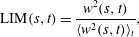 $$\begin{eqnarray}\text{LIM}(s,t)=\frac{w^{2}(s,t)}{\langle w^{2}(s,t)\rangle _{t}},\end{eqnarray}$$
where the symbol
 $\langle \;\rangle _{t}$
denotes a time average. This function enhances non-uniform distributions of energy in time because the quantity
$\langle \;\rangle _{t}$
denotes a time average. This function enhances non-uniform distributions of energy in time because the quantity
 $w^{2}(s,t)$
can be interpreted as the energy contained in the signal at the scale
$w^{2}(s,t)$
can be interpreted as the energy contained in the signal at the scale
 $s$
and the instant
$s$
and the instant
 $t$
(Pagliaroli et al.
Reference Pagliaroli, Camussi, Giacomazzi and Giulietti2015).
$t$
(Pagliaroli et al.
Reference Pagliaroli, Camussi, Giacomazzi and Giulietti2015).
Camussi & Guj (Reference Camussi and Guj1997) introduced a coherent structures identification procedure based on the idea that the passage of a high-energy flow structure of a characteristic size
 $s_{i}$
at the instant
$s_{i}$
at the instant
 $t_{k}$
should induce a burst in the LIM at the corresponding time scale location. The LIM can be thresholded, fixing a proper trigger level
$t_{k}$
should induce a burst in the LIM at the corresponding time scale location. The LIM can be thresholded, fixing a proper trigger level
 $T$
, to select relative maxima which satisfy the condition
$T$
, to select relative maxima which satisfy the condition
 $\text{LIM}(s_{i},t_{k})>T$
.
$\text{LIM}(s_{i},t_{k})>T$
.
Once reference time instants
 $t_{k}^{\ast }$
fulfilling the triggering condition are selected, a set of signal segments centred on the time instants
$t_{k}^{\ast }$
fulfilling the triggering condition are selected, a set of signal segments centred on the time instants
 $t_{k}^{\ast }$
is extracted and an ensemble average of the set is performed revealing the time signatures hidden in the original signal. The independence of the educed signatures from the selected threshold level
$t_{k}^{\ast }$
is extracted and an ensemble average of the set is performed revealing the time signatures hidden in the original signal. The independence of the educed signatures from the selected threshold level
 $T$
has been verified (see also Camussi et al.
Reference Camussi, Grilliat, Caputi Gennaro and Jacob2010).
$T$
has been verified (see also Camussi et al.
Reference Camussi, Grilliat, Caputi Gennaro and Jacob2010).
The procedure is applied to the time signals of the present experiment and a description of the selection process illustrated above is depicted in figure 3. As an example, the wall pressure signal at an axial distance
 $x/D=10$
for a jet–plate distance
$x/D=10$
for a jet–plate distance
 $H/D=1$
has been considered. Figure 3(a) represents the time–frequency map of the LIM; the pseudo-frequencies, which are inversely proportional to the scales, are expressed in terms of a Strouhal number based on the nozzle diameter and the jet velocity. For each scale (or frequency), the time instants of the most energetic events are identified by the relative maxima exceeding a threshold level (figure 3
b). The resulting set of events allows the extraction of centred portions of signal (dashed rectangles in figure 3
c) from the original time series that are used to perform the ensemble average.
$H/D=1$
has been considered. Figure 3(a) represents the time–frequency map of the LIM; the pseudo-frequencies, which are inversely proportional to the scales, are expressed in terms of a Strouhal number based on the nozzle diameter and the jet velocity. For each scale (or frequency), the time instants of the most energetic events are identified by the relative maxima exceeding a threshold level (figure 3
b). The resulting set of events allows the extraction of centred portions of signal (dashed rectangles in figure 3
c) from the original time series that are used to perform the ensemble average.

Figure 3. Example of the selection procedure of the most energetic events in a time signal based on the LIM computation. (a) Time–frequency map of the LIM. (b) One-dimensional plot of the LIM at a given scale/frequency; the local maxima are highlighted with a circle whereas the trigger threshold level is represented by a dash-dotted line. (c) Portion of the wall pressure signal; the segments corresponding to large values of the LIM are highlighted with a dashed-line window.
3.1 Auto-conditioning procedure
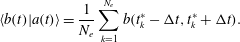
The auto-conditioning procedure is based on the selection of events from a time signal
 $a(t)$
and the conditional average of the signal itself. As a result, the educed time signature represents the shape of the flow structure embedded in the chaotic signal. The ensemble average of the signal segments centred in time at the instants
$a(t)$
and the conditional average of the signal itself. As a result, the educed time signature represents the shape of the flow structure embedded in the chaotic signal. The ensemble average of the signal segments centred in time at the instants
 $t_{k}^{\ast }$
corresponding to high-energy events is performed according to the following formula:
$t_{k}^{\ast }$
corresponding to high-energy events is performed according to the following formula:
 $$\begin{eqnarray}\langle a(t)|a(t)\rangle =\frac{1}{N_{e}}\mathop{\sum }_{k=1}^{N_{e}}a(t_{k}^{\ast }-\unicode[STIX]{x0394}t,t_{k}^{\ast }+\unicode[STIX]{x0394}t),\end{eqnarray}$$
where
 $N_{e}$
is the number of events corresponding to the condition
$N_{e}$
is the number of events corresponding to the condition
 $\text{LIM}(s_{i},t_{k})>T$
and
$\text{LIM}(s_{i},t_{k})>T$
and
 $\unicode[STIX]{x0394}t$
is a proper time window dependent on the estimated persistence of the effect of the detected singularity (see Camussi & Guj Reference Camussi and Guj1999). In the present approach
$\unicode[STIX]{x0394}t$
is a proper time window dependent on the estimated persistence of the effect of the detected singularity (see Camussi & Guj Reference Camussi and Guj1999). In the present approach
 $\unicode[STIX]{x0394}t$
was selected one order of magnitude greater than the integral time scale of the signal
$\unicode[STIX]{x0394}t$
was selected one order of magnitude greater than the integral time scale of the signal
 $a(t)$
. The integral time scale was evaluated as the first zero of the autocorrelation function, its value being larger for increasing axial distances as an effect of the turbulence development in the jet.
$a(t)$
. The integral time scale was evaluated as the first zero of the autocorrelation function, its value being larger for increasing axial distances as an effect of the turbulence development in the jet.
In the present work the auto-conditioning procedure has been applied to wall pressure and velocity signals for all the jet–plate configurations at different axial and transverse positions.
3.2 Cross-conditioning procedure
The conditioning method described above can be applied to two signals acquired simultaneously. The ensemble average of signal segments
 $b(t)$
conditioned on
$b(t)$
conditioned on
 $a(t)$
and centred in time at instants
$a(t)$
and centred in time at instants
 $t_{k}^{\ast }$
is calculated according to the following formula:
$t_{k}^{\ast }$
is calculated according to the following formula:
 $$\begin{eqnarray}\langle b(t)|a(t)\rangle =\frac{1}{N_{e}}\mathop{\sum }_{k=1}^{N_{e}}b(t_{k}^{\ast }-\unicode[STIX]{x0394}t,t_{k}^{\ast }+\unicode[STIX]{x0394}t).\end{eqnarray}$$
The educed signatures
 $\langle b(t)\rangle$
represent the shape of the coherent content of
$\langle b(t)\rangle$
represent the shape of the coherent content of
 $b(t)$
responsible for energetic events in the signal
$b(t)$
responsible for energetic events in the signal
 $a(t)$
.
$a(t)$
.
Furthermore, the time delay associated with the extracted ensemble average can be retrieved providing information on the propagation velocity of the educed structure between the measurement points of the two signals (Guj et al. Reference Guj, Carley, Camussi and Ragni2003; Camussi et al. Reference Camussi, Grilliat, Caputi Gennaro and Jacob2010).
In the present approach the triggering signal
 $a(t)$
is given by the wall pressure time series, whereas the conditioned signals
$a(t)$
is given by the wall pressure time series, whereas the conditioned signals
 $b(t)$
were either wall pressure signals measured by another microphone of the array or a velocity signal measured by the hot-wire anemometer.
$b(t)$
were either wall pressure signals measured by another microphone of the array or a velocity signal measured by the hot-wire anemometer.
4 Results
4.1 Effect of the flat plate on the velocity field
In this section the effect of the flat plate on the aerodynamic field is characterized. As previously reported in Di Marco et al. (Reference Di Marco, Mancinelli and Camussi2015), the flat plate affects both the mean and fluctuating aerodynamic fields inducing a modification of the axisymmetry of the jet and a reduction of the velocity fluctuation intensity in the proximity of the surface.
The installation effect of the surface on the velocity field is analysed in terms of variation of the statistical moments up to the fourth order in the plane
 $x$
–
$x$
–
 $z$
, i.e. the plane orthogonal to the plate and parallel to the nozzle axis (see figure 2). The description of the velocity field statistics in terms of external aerodynamic variables is achieved by pointwise HW anemometer measurements.
$z$
, i.e. the plane orthogonal to the plate and parallel to the nozzle axis (see figure 2). The description of the velocity field statistics in terms of external aerodynamic variables is achieved by pointwise HW anemometer measurements.
Figure 4 shows the contour maps of the dimensionless mean velocity field for all the jet–plate configurations. The mean velocity is normalized by the jet velocity
 $U_{j}$
, whereas the axial distance
$U_{j}$
, whereas the axial distance
 $x$
and the transverse distance
$x$
and the transverse distance
 $z$
are divided by the nozzle diameter
$z$
are divided by the nozzle diameter
 $D$
. It can be observed that the jet bends over the surface for all the plate radial distances, such a behaviour being ascribed to the so-called Coanda effect (Bourque & Newman Reference Bourque and Newman1960; Wille & Fernholz Reference Wille and Fernholz1965; Launder & Rodi Reference Launder and Rodi1983). The Coanda effect is strongly dependent on the parameter
$D$
. It can be observed that the jet bends over the surface for all the plate radial distances, such a behaviour being ascribed to the so-called Coanda effect (Bourque & Newman Reference Bourque and Newman1960; Wille & Fernholz Reference Wille and Fernholz1965; Launder & Rodi Reference Launder and Rodi1983). The Coanda effect is strongly dependent on the parameter
 $H$
, the jet deflection being more significant as the flat plate gets closer to the jet. This result is further highlighted in figure 5, which shows the shift of the jet axis along the axial direction. The presence of the flat plate induces the departure of the jet axis from the geometrical nozzle axis. The jet axis is defined hereinafter as the
$H$
, the jet deflection being more significant as the flat plate gets closer to the jet. This result is further highlighted in figure 5, which shows the shift of the jet axis along the axial direction. The presence of the flat plate induces the departure of the jet axis from the geometrical nozzle axis. The jet axis is defined hereinafter as the
 $z$
-positions, a function of the axial distance
$z$
-positions, a function of the axial distance
 $x$
, where the maximum values of the mean velocity were measured. It is interesting to note that, for low streamwise positions, the maximum velocity value is measured in the jet side opposite to the flat plate, as extensively discussed in Di Marco et al. (Reference Di Marco, Mancinelli and Camussi2015).
$x$
, where the maximum values of the mean velocity were measured. It is interesting to note that, for low streamwise positions, the maximum velocity value is measured in the jet side opposite to the flat plate, as extensively discussed in Di Marco et al. (Reference Di Marco, Mancinelli and Camussi2015).
It has to be pointed out that the Coanda effect is expected to be weaker in flight conditions, the deformation of the mean aerodynamic field being thus reduced in a real aircraft configuration. Further investigations with a background ‘flight’ stream velocity have to be carried out in order to clarify this aspect.

Figure 4. Dimensionless mean velocity field in the plane
 $x$
–
$x$
–
 $z$
for all the jet–plate configurations: (a)
$z$
for all the jet–plate configurations: (a)
 $H/D=1$
, (b)
$H/D=1$
, (b)
 $H/D=1.5$
, (c)
$H/D=1.5$
, (c)
 $H/D=2$
, (d)
$H/D=2$
, (d)
 $H/D=2.5$
. Dash-dotted lines represent the nozzle axis.
$H/D=2.5$
. Dash-dotted lines represent the nozzle axis.

Figure 5. Plate effect on mean velocity field. Shift of the jet axis along the axial distance for: ♢,
 $H/D=1$
; ○,
$H/D=1$
; ○,
 $H/D=1.5$
; ▫,
$H/D=1.5$
; ▫,
 $H/D=2$
; ▵,
$H/D=2$
; ▵,
 $H/D=2.5$
. The bold dash-dotted line refers to the geometrical nozzle axis.
$H/D=2.5$
. The bold dash-dotted line refers to the geometrical nozzle axis.
The plate effect on the fluctuating velocity field is provided in figure 6, which shows the contour maps of the streamwise turbulence intensity. This quantity was computed by dividing the velocity standard deviation by the maximum mean velocity value at each axial distance. It is observed that the plate induces an asymmetry of the turbulence intensity, the velocity fluctuations being reduced in the jet region close to the surface. Such an effect is stronger for closer jet–plate configurations. Furthermore, the turbulence level globally lowers as the surface distance decreases.

Figure 6. Streamwise turbulence intensity field in the plane
 $x$
–
$x$
–
 $z$
for all the jet–plate distances: (a)
$z$
for all the jet–plate distances: (a)
 $H/D=1$
, (b)
$H/D=1$
, (b)
 $H/D=1.5$
, (c)
$H/D=1.5$
, (c)
 $H/D=2$
, (d)
$H/D=2$
, (d)
 $H/D=2.5$
. Dash-dotted lines represent the nozzle axis.
$H/D=2.5$
. Dash-dotted lines represent the nozzle axis.
The statistical description of the jet–plate interaction is further provided by the evolution of higher-order statistical moments of the velocity field. Figure 7 shows the contour maps of the skewness factor of the streamwise velocity component. It is observed that the third-order statistical moment is close to 0 in the jet plume except for the internal and external shear layer regions where negative and positive values respectively are found. The positive skewness values in the outer shear layers can be ascribed to positive velocity fluctuations due to the injection of ambient flow associated with the entrainment effect of the jet. Conversely, the distribution of the negative skewness values clearly defines the potential core shape. Figure 8 shows the contour maps of the flatness factor of the streamwise velocity component. The fourth-order statistical moment is close to 3 in the jet plume except for the outer and inner shear layers where larger kurtosis values associated with regions of strong intermittency are found. It can be noted that the effect of the plate is to prevent the development of the outer shear layer in the jet side close to the surface, thus reducing the generation of intermittent events which are strictly related to the turbulence production. Such inference is further supported by the reduction of the turbulence intensity observed in figure 6.

Figure 7. Skewness factor of the axial velocity field in the plane
 $x$
–
$x$
–
 $z$
for all the jet–plate configurations: (a)
$z$
for all the jet–plate configurations: (a)
 $H/D=1$
, (b)
$H/D=1$
, (b)
 $H/D=1.5$
, (c)
$H/D=1.5$
, (c)
 $H/D=2$
, (d)
$H/D=2$
, (d)
 $H/D=2.5$
. Dash-dotted lines represent the nozzle axis.
$H/D=2.5$
. Dash-dotted lines represent the nozzle axis.

Figure 8. Flatness factor of the axial velocity field in the plane
 $x$
–
$x$
–
 $z$
for all the jet–plate configurations: (a)
$z$
for all the jet–plate configurations: (a)
 $H/D=1$
, (b)
$H/D=1$
, (b)
 $H/D=1.5$
, (c)
$H/D=1.5$
, (c)
 $H/D=2$
, (d)
$H/D=2$
, (d)
 $H/D=2.5$
. Dash-dotted lines represent the nozzle axis.
$H/D=2.5$
. Dash-dotted lines represent the nozzle axis.
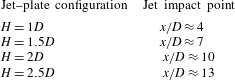
From the overall aerodynamic characterization, it has been verified that the potential core length, that is around
 $6D$
(Di Marco et al.
Reference Di Marco, Mancinelli and Camussi2015), is not significantly affected by the presence of the plate, this result not being reported for the sake of brevity. In order to better appreciate the results provided in the following sections, the jet impact points on the surface for all the jet–plate configurations evaluated by the HW measurements are reported in table 2 (for more details see Di Marco et al.
Reference Di Marco, Mancinelli and Camussi2015).
$6D$
(Di Marco et al.
Reference Di Marco, Mancinelli and Camussi2015), is not significantly affected by the presence of the plate, this result not being reported for the sake of brevity. In order to better appreciate the results provided in the following sections, the jet impact points on the surface for all the jet–plate configurations evaluated by the HW measurements are reported in table 2 (for more details see Di Marco et al.
Reference Di Marco, Mancinelli and Camussi2015).
Table 2. Summary of the axial distances for which the jet impinges on the plate for all the surface radial distances.
4.2 Cross-statistics between velocity and wall pressure fields
Cross-correlations and cross-spectra of velocity and wall pressure signals are presented addressing the effect of the plate distance from the jet as well as the positions of the hot wire and microphones. The velocity/pressure cross-statistics are obtained according to the scheme depicted in figure 9. Specifically, pressure signals from the microphone in the
 $i$
th axial position are correlated with velocity signals obtained by the hot-wire probe in the
$i$
th axial position are correlated with velocity signals obtained by the hot-wire probe in the
 $(i-1)$
th axial position.
$(i-1)$
th axial position.

Figure 9. Sketch of the hot wire and microphone disposition for the computation of the cross-correlations and cross-spectra.
4.2.1 Cross-correlations
The cross-correlation between axial velocity and wall pressure signals is computed according to the following formula (Di Marco et al. Reference Di Marco, Mancinelli and Camussi2015):
 $$\begin{eqnarray}R_{u_{i}p_{i+1}}(\unicode[STIX]{x1D709},\unicode[STIX]{x1D70F})=\langle u(x,t)p(x+\unicode[STIX]{x1D709},t+\unicode[STIX]{x1D70F})\rangle ,\end{eqnarray}$$
where
 $\unicode[STIX]{x1D709}$
is the streamwise distance between the hot wire and the microphone (in the present study
$\unicode[STIX]{x1D709}$
is the streamwise distance between the hot wire and the microphone (in the present study
 $\unicode[STIX]{x1D709}=1D$
) and
$\unicode[STIX]{x1D709}=1D$
) and
 $\unicode[STIX]{x1D70F}$
is the time lag. The cross-correlation coefficient
$\unicode[STIX]{x1D70F}$
is the time lag. The cross-correlation coefficient
 $\unicode[STIX]{x1D70C}_{u_{i}p_{i+1}}$
is obtained by normalizing the cross-correlation by the product between the standard deviations of the velocity and wall pressure signals.
$\unicode[STIX]{x1D70C}_{u_{i}p_{i+1}}$
is obtained by normalizing the cross-correlation by the product between the standard deviations of the velocity and wall pressure signals.
Figure 10 shows the cross-correlation coefficient between the velocity and wall pressure signals at different axial positions of the hot-wire probe:
 $x/D=4$
, 9, 16 and 23 for the plate position closest to the jet, i.e.
$x/D=4$
, 9, 16 and 23 for the plate position closest to the jet, i.e.
 $H/D=1$
. Three different locations of the hot wire on the
$H/D=1$
. Three different locations of the hot wire on the
 $z$
-axis are shown: the closest distance to the plate (denoted as
$z$
-axis are shown: the closest distance to the plate (denoted as
 $\unicode[STIX]{x1D701}$
), the nozzle axis position (
$\unicode[STIX]{x1D701}$
), the nozzle axis position (
 $z=0$
) and the jet axis position, as formally defined in § 4.1. It can be observed that both the amplitude and the shape of the correlation change depending on the axial and transverse positions. For
$z=0$
) and the jet axis position, as formally defined in § 4.1. It can be observed that both the amplitude and the shape of the correlation change depending on the axial and transverse positions. For
 $x/D=4$
an oscillatory shape can be found for all the
$x/D=4$
an oscillatory shape can be found for all the
 $z$
-positions. Moving downstream within the jet plume, the turbulence intensity increases and the shape of the correlation changes accordingly, showing a larger time scale related to the development of large turbulent structures. For the HW transverse locations corresponding to the nozzle and jet axes, the correlation exhibits a positive–negative bump. Conversely, a significant variation of the correlation trend is detected for the probe position closest to the plate. A dominant positive bump is clearly observed for the axial positions
$z$
-positions. Moving downstream within the jet plume, the turbulence intensity increases and the shape of the correlation changes accordingly, showing a larger time scale related to the development of large turbulent structures. For the HW transverse locations corresponding to the nozzle and jet axes, the correlation exhibits a positive–negative bump. Conversely, a significant variation of the correlation trend is detected for the probe position closest to the plate. A dominant positive bump is clearly observed for the axial positions
 $x/D=9$
and 16, the correlation maximum being located at a time delay corresponding to the negative peak of the correlation associated with the nozzle and jet axis positions. For axial distances further downstream in the jet plume a positive–negative bump is also found for the transverse position
$x/D=9$
and 16, the correlation maximum being located at a time delay corresponding to the negative peak of the correlation associated with the nozzle and jet axis positions. For axial distances further downstream in the jet plume a positive–negative bump is also found for the transverse position
 $\unicode[STIX]{x1D701}$
, the positive peak still being located corresponding to the negative one related to the nozzle/jet axis position. An overview of the crosswise evolution of the correlation between velocity and wall pressure signals for
$\unicode[STIX]{x1D701}$
, the positive peak still being located corresponding to the negative one related to the nozzle/jet axis position. An overview of the crosswise evolution of the correlation between velocity and wall pressure signals for
 $H/D=1$
is reported in figure 11, which shows the cross-correlation coefficient maps along the
$H/D=1$
is reported in figure 11, which shows the cross-correlation coefficient maps along the
 $z$
-axis for the same axial positions listed above. It is observed that the highest correlation level is found for transverse positions in the proximity of the nozzle axis. Furthermore the correlation shape changes as the hot wire approaches the flat plate. Such different correlation trends could be ascribed to a phase shift, the axial velocity and wall pressure signals being in phase opposition for crosswise locations close to the nozzle axis and in phase for transverse positions close to the plate (Lau, Fisher & Fuchs Reference Lau, Fisher and Fuchs1972).
$z$
-axis for the same axial positions listed above. It is observed that the highest correlation level is found for transverse positions in the proximity of the nozzle axis. Furthermore the correlation shape changes as the hot wire approaches the flat plate. Such different correlation trends could be ascribed to a phase shift, the axial velocity and wall pressure signals being in phase opposition for crosswise locations close to the nozzle axis and in phase for transverse positions close to the plate (Lau, Fisher & Fuchs Reference Lau, Fisher and Fuchs1972).

Figure 10. Cross-correlation coefficient between velocity and wall pressure signals for
 $H/D=1$
at axial positions: (a) HW
$H/D=1$
at axial positions: (a) HW
 $x/D=4$
, MIC
$x/D=4$
, MIC
 $x/D=5$
; (b) HW
$x/D=5$
; (b) HW
 $x/D=9$
, MIC
$x/D=9$
, MIC
 $x/D=10$
; (c) HW
$x/D=10$
; (c) HW
 $x/D=16$
, MIC
$x/D=16$
, MIC
 $x/D=17$
; (d) HW
$x/D=17$
; (d) HW
 $x/D=23$
, MIC
$x/D=23$
, MIC
 $x/D=24$
. HW transverse locations: solid lines refer to the position
$x/D=24$
. HW transverse locations: solid lines refer to the position
 $\unicode[STIX]{x1D701}$
, dashed lines to the nozzle axis, dotted lines to the jet axis.
$\unicode[STIX]{x1D701}$
, dashed lines to the nozzle axis, dotted lines to the jet axis.
Figure 11. Cross-correlation coefficient maps along the
 $z$
-axis between axial velocity and wall pressure signals for the plate radial distance
$z$
-axis between axial velocity and wall pressure signals for the plate radial distance
 $H/D=1$
: (a) HW
$H/D=1$
: (a) HW
 $x/D=4$
, MIC
$x/D=4$
, MIC
 $x/D=5$
; (b) HW
$x/D=5$
; (b) HW
 $x/D=9$
, MIC
$x/D=9$
, MIC
 $x/D=10$
; (c) HW
$x/D=10$
; (c) HW
 $x/D=16$
, MIC
$x/D=16$
, MIC
 $x/D=17$
; (d) HW
$x/D=17$
; (d) HW
 $x/D=23$
, MIC
$x/D=23$
, MIC
 $x/D=24$
.
$x/D=24$
.
Figure 12 shows the cross-correlation coefficient maps along the
 $x$
-axis for all
$x$
-axis for all
 $H$
. The hot-wire location on the
$H$
. The hot-wire location on the
 $z$
-axis corresponds to the jet axis position for each axial distance considered. According to Fuchs (Reference Fuchs1972), the correlation coefficient exhibits a narrow oscillatory shape for small streamwise positions within the potential core region. Such a pseudo-periodic behaviour is ascribed to the signature of the Kelvin–Helmholtz instability. As illustrated above, moving downstream in the jet plume the turbulence development produces a positive–negative bump shape whose time scale enlarges as the axial distance increases. Such a trend is in agreement with the results presented by Henning, Koop & Schröder (Reference Henning, Koop and Schröder2013) for the case of a free jet. It has to be underlined that for
$z$
-axis corresponds to the jet axis position for each axial distance considered. According to Fuchs (Reference Fuchs1972), the correlation coefficient exhibits a narrow oscillatory shape for small streamwise positions within the potential core region. Such a pseudo-periodic behaviour is ascribed to the signature of the Kelvin–Helmholtz instability. As illustrated above, moving downstream in the jet plume the turbulence development produces a positive–negative bump shape whose time scale enlarges as the axial distance increases. Such a trend is in agreement with the results presented by Henning, Koop & Schröder (Reference Henning, Koop and Schröder2013) for the case of a free jet. It has to be underlined that for
 $H/D=1$
the highest correlation value is found in the potential core region. On the contrary, for larger values of
$H/D=1$
the highest correlation value is found in the potential core region. On the contrary, for larger values of
 $H$
, the maximum correlation level is observed for axial positions increasingly further from the nozzle exhaust. Globally, the correlation amplitude decreases as the flat plate is moved away from the jet.
$H$
, the maximum correlation level is observed for axial positions increasingly further from the nozzle exhaust. Globally, the correlation amplitude decreases as the flat plate is moved away from the jet.
The cross-correlation coefficient maps along the axial distance for all the flat-plate radial distances and for the hot-wire transverse position
 $\unicode[STIX]{x1D701}$
are shown in figure 13. The correlation close to the nozzle exhaust decreases for increasing
$\unicode[STIX]{x1D701}$
are shown in figure 13. The correlation close to the nozzle exhaust decreases for increasing
 $H$
and becomes negligible for the largest plate distance, i.e.
$H$
and becomes negligible for the largest plate distance, i.e.
 $H/D=2.5$
. This behaviour is ascribed to the relation between
$H/D=2.5$
. This behaviour is ascribed to the relation between
 $H$
and the axial position where the jet impacts the surface. Specifically, non-zero correlation values are found for axial positions in the proximity of and beyond the impact point. For such positions positive–negative bump shape correlations are found, whereas as the flow develops over the surface a positive bump shape correlation clearly appears.
$H$
and the axial position where the jet impacts the surface. Specifically, non-zero correlation values are found for axial positions in the proximity of and beyond the impact point. For such positions positive–negative bump shape correlations are found, whereas as the flow develops over the surface a positive bump shape correlation clearly appears.

Figure 12. Cross-correlation coefficient maps along the axial distance for hot-wire transverse positions corresponding to the jet axis. Flat-plate radial distance: (a)
 $H/D=1$
; (b)
$H/D=1$
; (b)
 $H/D=1.5$
; (c)
$H/D=1.5$
; (c)
 $H/D=2$
; (d)
$H/D=2$
; (d)
 $H/D=2.5$
.
$H/D=2.5$
.

Figure 13. Cross-correlation coefficient maps along the axial distance for hot-wire transverse position
 $\unicode[STIX]{x1D701}$
. Flat-plate radial distance: (a)
$\unicode[STIX]{x1D701}$
. Flat-plate radial distance: (a)
 $H/D=1$
; (b)
$H/D=1$
; (b)
 $H/D=1.5$
; (c)
$H/D=1.5$
; (c)
 $H/D=2$
; (d)
$H/D=2$
; (d)
 $H/D=2.5$
.
$H/D=2.5$
.
The effect of
 $H/D$
on the correlation is shown in figure 14, which shows the cross-correlation coefficient at the HW axial distances
$H/D$
on the correlation is shown in figure 14, which shows the cross-correlation coefficient at the HW axial distances
 $x/D=4$
, 9, 16 and 23 and for the hot-wire transverse location on the jet axis. It can be seen that the evolution along the streamwise direction described above is not significantly affected by the radial distance
$x/D=4$
, 9, 16 and 23 and for the hot-wire transverse location on the jet axis. It can be seen that the evolution along the streamwise direction described above is not significantly affected by the radial distance
 $H$
. A stronger effect is detected considering the correlation for the hot-wire position closest to the flat plate. Figure 15 shows the cross-correlation coefficient for the hot-wire position
$H$
. A stronger effect is detected considering the correlation for the hot-wire position closest to the flat plate. Figure 15 shows the cross-correlation coefficient for the hot-wire position
 $\unicode[STIX]{x1D701}$
at the axial positions
$\unicode[STIX]{x1D701}$
at the axial positions
 $x/D=2$
, 11, 17 and 24. It is observed that both the correlation amplitude and shape change as the axial distance increases. As reported above, zero-correlation values are found for small axial positions where the jet had not yet impinged on the surface. Moving away from the impact point, a predominant positive bump is detected, its shape being sharper for the smallest jet–plate distance. It is interesting to point out that for
$x/D=2$
, 11, 17 and 24. It is observed that both the correlation amplitude and shape change as the axial distance increases. As reported above, zero-correlation values are found for small axial positions where the jet had not yet impinged on the surface. Moving away from the impact point, a predominant positive bump is detected, its shape being sharper for the smallest jet–plate distance. It is interesting to point out that for
 $H/D\leqslant 1.5$
, a positive–negative bump shape appears again for large axial distances.
$H/D\leqslant 1.5$
, a positive–negative bump shape appears again for large axial distances.

Figure 14. Effect of the plate radial distance on the cross-correlation coefficient between velocity and wall pressure signals for the hot-wire transverse positions on the jet axis: (a) HW
 $x/D=4$
, MIC
$x/D=4$
, MIC
 $x/D=5$
; (b) HW
$x/D=5$
; (b) HW
 $x/D=9$
, MIC
$x/D=9$
, MIC
 $x/D=10$
; (c) HW
$x/D=10$
; (c) HW
 $x/D=16$
, MIC
$x/D=16$
, MIC
 $x/D=17$
; (d) HW
$x/D=17$
; (d) HW
 $x/D=23$
, MIC
$x/D=23$
, MIC
 $x/D=24$
. Solid lines refer to jet–plate distance
$x/D=24$
. Solid lines refer to jet–plate distance
 $H/D=1$
, dashed lines to
$H/D=1$
, dashed lines to
 $H/D=1.5$
, dotted lines to
$H/D=1.5$
, dotted lines to
 $H/D=2$
, and dash-dotted lines to
$H/D=2$
, and dash-dotted lines to
 $H/D=2.5$
.
$H/D=2.5$
.

Figure 15. Effect of the plate radial distance on the cross-correlation coefficient between velocity and wall pressure signals for the hot-wire transverse positions corresponding to
 $\unicode[STIX]{x1D701}$
: (a) HW
$\unicode[STIX]{x1D701}$
: (a) HW
 $x/D=2$
, MIC
$x/D=2$
, MIC
 $x/D=3$
; (b) HW
$x/D=3$
; (b) HW
 $x/D=11$
, MIC
$x/D=11$
, MIC
 $x/D=12$
; (c) HW
$x/D=12$
; (c) HW
 $x/D=17$
, MIC
$x/D=17$
, MIC
 $x/D=18$
; (d) HW
$x/D=18$
; (d) HW
 $x/D=24$
, MIC
$x/D=24$
, MIC
 $x/D=25$
. Solid lines refer to jet–plate distance
$x/D=25$
. Solid lines refer to jet–plate distance
 $H/D=1$
, dashed lines to
$H/D=1$
, dashed lines to
 $H/D=1.5$
, dotted lines to
$H/D=1.5$
, dotted lines to
 $H/D=2$
, and dash-dotted lines to
$H/D=2$
, and dash-dotted lines to
 $H/D=2.5$
.
$H/D=2.5$
.
4.2.2 Cross-spectra
The cross-spectrum between the axial velocity and the wall pressure signals is defined as the Fourier transform of the cross-correlation function, as formalized in the following:
 $$\begin{eqnarray}\unicode[STIX]{x1D6F7}_{u_{i}\,p_{i+1}}(\unicode[STIX]{x1D709},f)=\int _{-\infty }^{+\infty }R_{u_{i}\,p_{i+1}}(\unicode[STIX]{x1D709},\unicode[STIX]{x1D70F})\text{e}^{-j2\unicode[STIX]{x03C0}f\unicode[STIX]{x1D70F}}\,\text{d}\unicode[STIX]{x1D70F}.\end{eqnarray}$$
In the present approach the cross-spectrum was computed using Welch’s method with a Hamming window and an overlap of 50 %. A dimensionless cross-power spectral density (CPSD) was defined according to the following formula:
 $$\begin{eqnarray}\text{CPSD}=\frac{|\unicode[STIX]{x1D6F7}_{u_{i}\,p_{i+1}}|\,\unicode[STIX]{x0394}f_{ref}}{U_{j}\,p_{ref}},\end{eqnarray}$$
where
 $|\unicode[STIX]{x1D6F7}_{u_{i}\,p_{i+1}}|$
is the modulus of the cross-spectrum, and
$|\unicode[STIX]{x1D6F7}_{u_{i}\,p_{i+1}}|$
is the modulus of the cross-spectrum, and
 $\unicode[STIX]{x0394}f_{ref}$
and
$\unicode[STIX]{x0394}f_{ref}$
and
 $p_{ref}$
are a reference frequency and a reference pressure, whose values were set to 1 Hz and
$p_{ref}$
are a reference frequency and a reference pressure, whose values were set to 1 Hz and
 $20~\unicode[STIX]{x03BC}\text{Pa}$
, respectively.
$20~\unicode[STIX]{x03BC}\text{Pa}$
, respectively.
Figure 16 shows the CPSD map along the
 $z$
-axis for HW axial positions
$z$
-axis for HW axial positions
 $x/D=3$
, 7, 13 and 21. Since the dependence upon
$x/D=3$
, 7, 13 and 21. Since the dependence upon
 $H$
is weak, only the case
$H$
is weak, only the case
 $H/D=1$
is presented. The frequency is expressed in terms of Strouhal number based on
$H/D=1$
is presented. The frequency is expressed in terms of Strouhal number based on
 $D$
and
$D$
and
 $U_{j}$
at the nozzle exhaust. It is observed that for small axial distances within the potential core region the highest values of the cross-spectrum are found for transverse locations corresponding to the mixing layers of the jet. Furthermore, a tonal component for a Strouhal number
$U_{j}$
at the nozzle exhaust. It is observed that for small axial distances within the potential core region the highest values of the cross-spectrum are found for transverse locations corresponding to the mixing layers of the jet. Furthermore, a tonal component for a Strouhal number
 ${\approx}0.47$
is clearly detected for all the transverse positions. According to the outcome obtained from the velocity spectra reported in Di Marco et al. (Reference Di Marco, Mancinelli and Camussi2015) and in agreement with the trend shown in the cross-correlations, this signature is related to the Kelvin–Helmholtz instability mode. As the axial distance increases, the cross-spectral energy rises and spreads over a wider range of transverse positions, the maximum level being moved to lower frequencies and towards negative
${\approx}0.47$
is clearly detected for all the transverse positions. According to the outcome obtained from the velocity spectra reported in Di Marco et al. (Reference Di Marco, Mancinelli and Camussi2015) and in agreement with the trend shown in the cross-correlations, this signature is related to the Kelvin–Helmholtz instability mode. As the axial distance increases, the cross-spectral energy rises and spreads over a wider range of transverse positions, the maximum level being moved to lower frequencies and towards negative
 $z$
-coordinates, i.e. in the jet region closer to the surface.
$z$
-coordinates, i.e. in the jet region closer to the surface.

Figure 16. Dimensionless cross-power spectral density maps along the
 $z$
-direction for
$z$
-direction for
 $H/D=1$
at axial positions: (a) HW
$H/D=1$
at axial positions: (a) HW
 $x/D=3$
, MIC
$x/D=3$
, MIC
 $x/D=4$
; (b) HW
$x/D=4$
; (b) HW
 $x/D=7$
, MIC
$x/D=7$
, MIC
 $x/D=8$
; (c) HW
$x/D=8$
; (c) HW
 $x/D=13$
, MIC
$x/D=13$
, MIC
 $x/D=14$
; (d) HW
$x/D=14$
; (d) HW
 $x/D=21$
, MIC
$x/D=21$
, MIC
 $x/D=22$
.
$x/D=22$
.
The effect of
 $H$
on the cross-spectra is addressed in figure 17. The cross-spectra are computed at the jet axis positions for hot-wire axial positions
$H$
on the cross-spectra is addressed in figure 17. The cross-spectra are computed at the jet axis positions for hot-wire axial positions
 $x/D=3$
, 9, 17 and 22. It is observed that the energy content decreases as
$x/D=3$
, 9, 17 and 22. It is observed that the energy content decreases as
 $H$
increases, the amplitude discrepancy being more significant for small streamwise locations. As the axial distance increases, the cross-spectra tend to collapse. It is interesting to underline that for streamwise positions within the potential core, the energy peak associated with the Kelvin–Helmholtz instability is clearly detected, this signature being more significant as
$H$
increases, the amplitude discrepancy being more significant for small streamwise locations. As the axial distance increases, the cross-spectra tend to collapse. It is interesting to underline that for streamwise positions within the potential core, the energy peak associated with the Kelvin–Helmholtz instability is clearly detected, this signature being more significant as
 $H$
increases.
$H$
increases.
An overview of the streamwise evolution of the cross-spectral energy for velocity signals at transverse positions corresponding to the jet axis is reported in figure 18, for all
 $H/D$
. The amplitude of the cross-spectra increases for decreasing
$H/D$
. The amplitude of the cross-spectra increases for decreasing
 $H$
and the maximum cross-spectral energy moves from high to low frequencies as the axial distance increases. Such a trend is related to the development of larger turbulent eddies moving downstream in the jet plume, in agreement with the results shown up to now.
$H$
and the maximum cross-spectral energy moves from high to low frequencies as the axial distance increases. Such a trend is related to the development of larger turbulent eddies moving downstream in the jet plume, in agreement with the results shown up to now.

Figure 17. Effect of the plate radial distance from the jet on the cross-power spectral density between consecutive velocity and wall pressure signals at axial positions: (a) HW
 $x/D=3$
, MIC
$x/D=3$
, MIC
 $x/D=4$
; (b) HW
$x/D=4$
; (b) HW
 $x/D=9$
, MIC
$x/D=9$
, MIC
 $x/D=10$
; (c) HW
$x/D=10$
; (c) HW
 $x/D=16$
, MIC
$x/D=16$
, MIC
 $x/D=17$
; (d) HW
$x/D=17$
; (d) HW
 $x/D=22$
, MIC
$x/D=22$
, MIC
 $x/D=23$
. Solid lines refer to plate distance
$x/D=23$
. Solid lines refer to plate distance
 $H/D=1$
, dashed lines to
$H/D=1$
, dashed lines to
 $H/D=1.5$
, dotted lines to
$H/D=1.5$
, dotted lines to
 $H/D=2$
, and dash-dotted lines to
$H/D=2$
, and dash-dotted lines to
 $H/D=2.5$
.
$H/D=2.5$
.

Figure 18. Dimensionless cross-power spectral density maps along the
 $x$
-axis for hot-wire transverse positions corresponding to the jet axis. Flat-plate radial distance: (a)
$x$
-axis for hot-wire transverse positions corresponding to the jet axis. Flat-plate radial distance: (a)
 $H/D=1$
; (b)
$H/D=1$
; (b)
 $H/D=1.5$
; (c)
$H/D=1.5$
; (c)
 $H/D=2$
; (d)
$H/D=2$
; (d)
 $H/D=2.5$
.
$H/D=2.5$
.
4.3 Wavelet analysis
According to the conditioning procedure described in § 3, the auto- and cross-conditioned ensemble averages of velocity and wall pressure signals are presented here. The averaged signatures are reported throughout the paper in dimensionless form by dividing the amplitude by the standard deviation of the original signal.
4.3.1 Velocity auto-conditioning
The streamwise evolution along the nozzle axis of the averaged auto-conditioned velocity signatures is shown in figure 19 for all
 $H$
. The signatures change significantly with the axial position of the hot wire. In the potential core region, where the Kelvin–Helmholtz instability is dominant, an oscillating shape is detected. For streamwise positions immediately downstream of the potential core, a negative peak shape related to the transitional behaviour of the jet flow is detected (Camussi & Guj Reference Camussi and Guj1999). Further downstream in the jet plume a positive spike-shaped signature associated with coherent ring-like vortices is observed (Camussi & Guj Reference Camussi and Guj1997). The contour maps along the streamwise direction of the velocity signatures on the nozzle axis for all
$H$
. The signatures change significantly with the axial position of the hot wire. In the potential core region, where the Kelvin–Helmholtz instability is dominant, an oscillating shape is detected. For streamwise positions immediately downstream of the potential core, a negative peak shape related to the transitional behaviour of the jet flow is detected (Camussi & Guj Reference Camussi and Guj1999). Further downstream in the jet plume a positive spike-shaped signature associated with coherent ring-like vortices is observed (Camussi & Guj Reference Camussi and Guj1997). The contour maps along the streamwise direction of the velocity signatures on the nozzle axis for all
 $H$
are represented in figure 20. It is observed that in the proximity of the potential core end, i.e. for
$H$
are represented in figure 20. It is observed that in the proximity of the potential core end, i.e. for
 $x/D=5-6$
(Di Marco et al.
Reference Di Marco, Mancinelli and Camussi2015), the oscillating shape of the velocity signature is significantly enhanced. It is interesting to underline that the evolution of flow signatures seems not to be modified by the presence of the flat plate since the results are very similar to those obtained by Camussi & Guj (Reference Camussi and Guj1999) in analogous analyses carried out in a free-jet case.
$x/D=5-6$
(Di Marco et al.
Reference Di Marco, Mancinelli and Camussi2015), the oscillating shape of the velocity signature is significantly enhanced. It is interesting to underline that the evolution of flow signatures seems not to be modified by the presence of the flat plate since the results are very similar to those obtained by Camussi & Guj (Reference Camussi and Guj1999) in analogous analyses carried out in a free-jet case.

Figure 19. Axial evolution of the auto-conditioned velocity signatures along the nozzle axis for all the jet–plate configurations: (a)
 $H/D=1$
; (b)
$H/D=1$
; (b)
 $H/D=1.5$
; (c)
$H/D=1.5$
; (c)
 $H/D=2$
; (d)
$H/D=2$
; (d)
 $H/D=2.5$
. Solid lines refer to
$H/D=2.5$
. Solid lines refer to
 $x/D=2$
, dashed lines to
$x/D=2$
, dashed lines to
 $x/D=7$
, dotted lines to
$x/D=7$
, dotted lines to
 $x/D=12$
, dash-dotted lines to
$x/D=12$
, dash-dotted lines to
 $x/D=17$
, and bold lines to
$x/D=17$
, and bold lines to
 $x/D=22$
.
$x/D=22$
.

Figure 20. Contour maps of the auto-conditioned velocity signatures along the nozzle axis for all the jet–plate configurations: (a)
 $H/D=1$
; (b)
$H/D=1$
; (b)
 $H/D=1.5$
; (c)
$H/D=1.5$
; (c)
 $H/D=2$
; (d)
$H/D=2$
; (d)
 $H/D=2.5$
.
$H/D=2.5$
.
The same results are obtained for hot-wire locations along the jet axis, and are not presented here for the sake of brevity.
Different results are found for the HW transverse location closest to the flat plate, i.e. the position
 $\unicode[STIX]{x1D701}$
. Figure 21 shows the contour maps of the velocity signatures along the
$\unicode[STIX]{x1D701}$
. Figure 21 shows the contour maps of the velocity signatures along the
 $x$
-axis for all
$x$
-axis for all
 $H$
. Positive spike-shaped signatures emerge for all the surface radial distances only downstream of the jet impact point on the plate. It can be observed that both the amplitude and the characteristic time scale of the educed structures are larger in the proximity of the jet impact point.
$H$
. Positive spike-shaped signatures emerge for all the surface radial distances only downstream of the jet impact point on the plate. It can be observed that both the amplitude and the characteristic time scale of the educed structures are larger in the proximity of the jet impact point.

Figure 21. Contour maps of the auto-conditioned velocity signatures along the streamwise direction at the hot-wire transverse position
 $\unicode[STIX]{x1D701}$
for all the jet–plate configurations: (a)
$\unicode[STIX]{x1D701}$
for all the jet–plate configurations: (a)
 $H/D=1$
; (b)
$H/D=1$
; (b)
 $H/D=1.5$
; (c)
$H/D=1.5$
; (c)
 $H/D=2$
; (d)
$H/D=2$
; (d)
 $H/D=2.5$
.
$H/D=2.5$
.
The effect of the radial distance of the flat plate from the jet is addressed in figure 22, which shows the velocity signatures for the hot-wire position
 $\unicode[STIX]{x1D701}$
at the axial positions
$\unicode[STIX]{x1D701}$
at the axial positions
 $x/D=16$
, 18, 21 and 23. The streamwise positions were chosen so that the jet had already impacted the surface. It is observed that the amplitude of the velocity ensemble averages increases for increasing
$x/D=16$
, 18, 21 and 23. The streamwise positions were chosen so that the jet had already impacted the surface. It is observed that the amplitude of the velocity ensemble averages increases for increasing
 $H$
. Furthermore the characteristic time scale of the signatures enlarges as the jet–plate distance increases, thus implying that the associated flow structures are characterized by a larger scale. Hence, the flat plate has the effect of inducing the breakdown of the large-scale structures. The trend just described can explain the reduction of the turbulence intensity observed in figure 6 for low
$H$
. Furthermore the characteristic time scale of the signatures enlarges as the jet–plate distance increases, thus implying that the associated flow structures are characterized by a larger scale. Hence, the flat plate has the effect of inducing the breakdown of the large-scale structures. The trend just described can explain the reduction of the turbulence intensity observed in figure 6 for low
 $H$
values and is in agreement with previous results presented in Di Marco et al. (Reference Di Marco, Mancinelli and Camussi2015).
$H$
values and is in agreement with previous results presented in Di Marco et al. (Reference Di Marco, Mancinelli and Camussi2015).

Figure 22. Auto-conditioned velocity signatures at the hot-wire transverse position
 $\unicode[STIX]{x1D701}$
for all the flat-plate radial distances: (a) axial position
$\unicode[STIX]{x1D701}$
for all the flat-plate radial distances: (a) axial position
 $x/D=16$
; (b)
$x/D=16$
; (b)
 $x/D=18$
; (c)
$x/D=18$
; (c)
 $x/D=21$
; (d)
$x/D=21$
; (d)
 $x/D=23$
. Solid lines refer to
$x/D=23$
. Solid lines refer to
 $H/D=1$
, dashed lines to
$H/D=1$
, dashed lines to
 $H/D=1.5$
, dotted lines to
$H/D=1.5$
, dotted lines to
 $H/D=2$
, and dash-dotted lines to
$H/D=2$
, and dash-dotted lines to
 $H/D=2.5$
.
$H/D=2.5$
.
A scaling criterion was derived for the auto-conditioned velocity signatures at the hot-wire transverse position
 $\unicode[STIX]{x1D701}$
. The proposed scaling criterion is based on the external aerodynamic variables
$\unicode[STIX]{x1D701}$
. The proposed scaling criterion is based on the external aerodynamic variables
 $U_{c}$
and
$U_{c}$
and
 $U_{j}$
and the main geometrical length scale
$U_{j}$
and the main geometrical length scale
 $H$
. The convection velocity
$H$
. The convection velocity
 $U_{c}$
was estimated from the time delay of the cross-correlation peak between consecutive wall pressure signals in the streamwise direction, which depends on
$U_{c}$
was estimated from the time delay of the cross-correlation peak between consecutive wall pressure signals in the streamwise direction, which depends on
 $H/D$
as reported in Di Marco et al. (Reference Di Marco, Mancinelli and Camussi2015). The velocity signatures are normalized by multiplying by the ratio
$H/D$
as reported in Di Marco et al. (Reference Di Marco, Mancinelli and Camussi2015). The velocity signatures are normalized by multiplying by the ratio
 $U_{c}/U_{j}$
and dividing by the local standard deviation of the velocity signal. Conversely, the characteristic time scale to be adopted is related to the time needed for a fluid particle convected by the mean flow to reach the flat plate. Such a time scale is estimated by the ratio
$U_{c}/U_{j}$
and dividing by the local standard deviation of the velocity signal. Conversely, the characteristic time scale to be adopted is related to the time needed for a fluid particle convected by the mean flow to reach the flat plate. Such a time scale is estimated by the ratio
 $H/U_{c}$
. Accordingly, the adopted scaling is defined as follows:
$H/U_{c}$
. Accordingly, the adopted scaling is defined as follows:
 $$\begin{eqnarray}\displaystyle & \displaystyle \langle u_{i}|u_{i}\rangle ^{\ast }=\frac{\langle u_{i}|u_{i}\rangle }{\langle u_{i}^{\prime 2}\rangle ^{1/2}}\frac{U_{c}}{U_{j}}, & \displaystyle\end{eqnarray}$$
 $$\begin{eqnarray}\displaystyle & \displaystyle \unicode[STIX]{x1D70F}^{\ast }=\unicode[STIX]{x1D70F}\frac{U_{c}}{H}. & \displaystyle\end{eqnarray}$$
Figure 23 shows the scaled velocity signatures for all the jet–plate configurations. For the sake of brevity the results concerning the axial positions
 $x/D=18$
and
$x/D=18$
and
 $x/D=22$
only are shown. A good collapse is observed for all
$x/D=22$
only are shown. A good collapse is observed for all
 $H$
in terms of both amplitude and time scale, although a small discrepancy is detected for the closest flat-plate position (
$H$
in terms of both amplitude and time scale, although a small discrepancy is detected for the closest flat-plate position (
 $H/D=1$
). It has to be pointed out that the same scaling parameters have been successfully used to scale the wall pressure autospectra (Di Marco et al.
Reference Di Marco, Mancinelli and Camussi2015). Such a behaviour implies a significant result: the aerodynamic and geometrical variables adopted to scale both the velocity signatures and the spectral content of the wall pressure fluctuations are representative of the parameters governing the jet–plate interaction phenomenon.
$H/D=1$
). It has to be pointed out that the same scaling parameters have been successfully used to scale the wall pressure autospectra (Di Marco et al.
Reference Di Marco, Mancinelli and Camussi2015). Such a behaviour implies a significant result: the aerodynamic and geometrical variables adopted to scale both the velocity signatures and the spectral content of the wall pressure fluctuations are representative of the parameters governing the jet–plate interaction phenomenon.

Figure 23. Scaled auto-conditioned velocity signatures at the hot-wire transverse position
 $\unicode[STIX]{x1D701}$
for all the jet–plate distances. Axial positions: (a)
$\unicode[STIX]{x1D701}$
for all the jet–plate distances. Axial positions: (a)
 $x/D=18$
, (b)
$x/D=18$
, (b)
 $x/D=22$
. Solid lines refer to
$x/D=22$
. Solid lines refer to
 $H/D=1$
, dashed lines to
$H/D=1$
, dashed lines to
 $H/D=1.5$
, dotted lines to
$H/D=1.5$
, dotted lines to
 $H/D=2$
, and dash-dotted lines to
$H/D=2$
, and dash-dotted lines to
 $H/D=2.5$
.
$H/D=2.5$
.
4.3.2 Pressure auto-conditioning
The wall pressure signatures derived from the auto-conditioning technique are presented in the following. Concerning the wall pressure field, as pointed out by Jayasundera, Casarella & Russell (Reference Jayasundera, Casarella and Russell1996), two different organized flow motions can be associated with pressure events over the wall surface:
-
(i) an ejection motion associated with positive pressure events; and
-
(ii) a sweep motion associated with negative pressure events.
Figure 24 shows the contour maps of the wall pressure signatures along the streamwise direction for all the jet–plate distances. It is observed that no relevant signatures can be appreciated for axial positions close to the nozzle exhaust. For small streamwise positions a positive–negative bump related to a burst–sweep event (Dhanak, Dowling & Si Reference Dhanak, Dowling and Si1997) is detected, except for the furthest plate radial distance. As the axial distance increases and a TBL is established, a negative pressure drop associated with sweep motion is observed, as reported by Johansson, Her & Haritonidis (Reference Johansson, Her and Haritonidis1987) for an equilibrium TBL.

Figure 24. Contour maps along the streamwise direction of the wall pressure signatures derived from the auto-conditioning technique for all the jet–plate distances: (a)
 $H/D=1$
; (b)
$H/D=1$
; (b)
 $H/D=1.5$
; (c)
$H/D=1.5$
; (c)
 $H/D=2$
; (d)
$H/D=2$
; (d)
 $H/D=2.5$
.
$H/D=2.5$
.
The effect of
 $H$
on the educed structures is addressed in figure 25, which shows the pressure signatures at axial distances
$H$
on the educed structures is addressed in figure 25, which shows the pressure signatures at axial distances
 $x/D=5$
, 10, 13 and 18. The ensemble averages obtained for the largest value of
$x/D=5$
, 10, 13 and 18. The ensemble averages obtained for the largest value of
 $H$
are characterized by a larger time scale, such a trend being in agreement with the results presented in the previous sections. For small axial distances the signature amplitude is larger for lower
$H$
are characterized by a larger time scale, such a trend being in agreement with the results presented in the previous sections. For small axial distances the signature amplitude is larger for lower
 $H$
, whereas the opposite trend is detected further downstream in the jet plume. It is interesting to underline that the appearance of sweep or burst–sweep events is strongly related to the plate distance from the jet and the streamwise position considered. Such a behaviour is due to the relation between the jet–plate separation and the axial distance for which the jet impinges on the plate. Specifically ejection events were detected for low streamwise positions and small
$H$
, whereas the opposite trend is detected further downstream in the jet plume. It is interesting to underline that the appearance of sweep or burst–sweep events is strongly related to the plate distance from the jet and the streamwise position considered. Such a behaviour is due to the relation between the jet–plate separation and the axial distance for which the jet impinges on the plate. Specifically ejection events were detected for low streamwise positions and small
 $H/D$
(1, 1.5), whereas sweep motions are found for larger jet–plate and axial distances.
$H/D$
(1, 1.5), whereas sweep motions are found for larger jet–plate and axial distances.

Figure 25. Effect of the jet–plate distance on the auto-conditioned wall pressure signatures at different axial positions: (a)
 $x/D=5$
, (b)
$x/D=5$
, (b)
 $x/D=10$
, (c)
$x/D=10$
, (c)
 $x/D=13$
, (d)
$x/D=13$
, (d)
 $x/D=18$
. Solid lines refer to
$x/D=18$
. Solid lines refer to
 $H/D=1$
, dashed lines to
$H/D=1$
, dashed lines to
 $H/D=1.5$
, dotted lines to
$H/D=1.5$
, dotted lines to
 $H/D=2$
, and dash-dotted lines to
$H/D=2$
, and dash-dotted lines to
 $H/D=2.5$
.
$H/D=2.5$
.
4.3.3 Pressure/pressure cross-conditioning
The cross-conditioning procedure was applied using as triggering signal the wall pressure signal and as conditioned signal the wall pressure time series of an adjacent microphone. For the sake of brevity the results concerning the cross-conditioned wall pressure signatures are not extensively discussed, the shape and the axial evolution of the educed structures being similar to those obtained from the auto-conditioning procedure illustrated above. Figure 26 shows the streamwise evolution of the cross-conditioned wall pressure signatures for all
 $H$
. Positive–negative bumps are extracted for small axial distances and for
$H$
. Positive–negative bumps are extracted for small axial distances and for
 $H/D\leqslant 1.5$
, confirming the results discussed above. Negative drop signatures related to sweep motion are detected for larger axial positions and for
$H/D\leqslant 1.5$
, confirming the results discussed above. Negative drop signatures related to sweep motion are detected for larger axial positions and for
 $H/D>1.5$
, the shape being in agreement with the results obtained by Camussi, Robert & Jacob (Reference Camussi, Robert and Jacob2008) for a fully developed TBL. According to Guj et al. (Reference Guj, Carley, Camussi and Ragni2003), taking into account the separation distance between the microphones and the time delay of the signature, a phase velocity can be computed. The velocity values obtained are a fraction of the jet velocity
$H/D>1.5$
, the shape being in agreement with the results obtained by Camussi, Robert & Jacob (Reference Camussi, Robert and Jacob2008) for a fully developed TBL. According to Guj et al. (Reference Guj, Carley, Camussi and Ragni2003), taking into account the separation distance between the microphones and the time delay of the signature, a phase velocity can be computed. The velocity values obtained are a fraction of the jet velocity
 $U_{j}$
, thus implying that the educed signatures are associated with hydrodynamic turbulent structures convected by the mean flow (Camussi et al.
Reference Camussi, Robert and Jacob2008; Mancinelli et al.
Reference Mancinelli, Pagliaroli, Di Marco, Camussi, Castelain and Léon2016b
).
$U_{j}$
, thus implying that the educed signatures are associated with hydrodynamic turbulent structures convected by the mean flow (Camussi et al.
Reference Camussi, Robert and Jacob2008; Mancinelli et al.
Reference Mancinelli, Pagliaroli, Di Marco, Camussi, Castelain and Léon2016b
).

Figure 26. Streamwise evolution of the cross-conditioned wall pressure signatures for four flat-plate radial distances. (a)
 $H/D=1$
; solid line refers to MIC axial position
$H/D=1$
; solid line refers to MIC axial position
 $x/D=6$
, dashed line
$x/D=6$
, dashed line
 $x/D=9$
, dotted line
$x/D=9$
, dotted line
 $x/D=12$
, dash-dotted line
$x/D=12$
, dash-dotted line
 $x/D=16$
. (b)
$x/D=16$
. (b)
 $H/D=1.5$
; solid line
$H/D=1.5$
; solid line
 $x/D=9$
, dashed line
$x/D=9$
, dashed line
 $x/D=12$
, dotted line
$x/D=12$
, dotted line
 $x/D=15$
, dash-dotted line
$x/D=15$
, dash-dotted line
 $x/D=17$
. (c)
$x/D=17$
. (c)
 $H/D=2$
: solid line
$H/D=2$
: solid line
 $x/D=12$
, dashed line
$x/D=12$
, dashed line
 $x/D=13$
, dotted line
$x/D=13$
, dotted line
 $x/D=15$
, dash-dotted line
$x/D=15$
, dash-dotted line
 $x/D=17$
. (d)
$x/D=17$
. (d)
 $H/D=2.5$
; solid line
$H/D=2.5$
; solid line
 $x/D=15$
, dashed line
$x/D=15$
, dashed line
 $x/D=16$
, dotted line
$x/D=16$
, dotted line
 $x/D=17$
, dash-dotted line
$x/D=17$
, dash-dotted line
 $x/D=23$
.
$x/D=23$
.
4.3.4 Velocity/pressure cross-conditioning
The velocity conditioned on the wall pressure is presented in the following. Figure 27 shows the shape of the educed flow structures for all the jet–plate configurations addressing the effect of the streamwise separation between the probes. The velocity signal measured at
 $\unicode[STIX]{x1D701}$
and
$\unicode[STIX]{x1D701}$
and
 $x/D=21$
is conditioned on the pressure signals from the microphones placed at
$x/D=21$
is conditioned on the pressure signals from the microphones placed at
 $x/D=22$
, 23, 24 and 25. It is observed that the extracted signatures are represented by a positive spike, whose shape can be ascribed to a ring-like vortex convected by the mean flow. The time shift associated with the signature peaks changes depending on the distance between the probes. Such a behaviour implies that the conditioning procedure adopted can provide information about the location of the extracted structures and track their spatial evolution. Furthermore, it is interesting to underline that the amplitude of the averaged signatures decreases as the distance between the hot wire and the microphone increases. Nevertheless, a non-zero signature is detected also for the largest separation distance (
$x/D=22$
, 23, 24 and 25. It is observed that the extracted signatures are represented by a positive spike, whose shape can be ascribed to a ring-like vortex convected by the mean flow. The time shift associated with the signature peaks changes depending on the distance between the probes. Such a behaviour implies that the conditioning procedure adopted can provide information about the location of the extracted structures and track their spatial evolution. Furthermore, it is interesting to underline that the amplitude of the averaged signatures decreases as the distance between the hot wire and the microphone increases. Nevertheless, a non-zero signature is detected also for the largest separation distance (
 $4D$
) between the probes. This result suggests that the flow structures responsible for the most energetic events in the wall pressure signals are represented by large vortices whose spatial coherence is significant in the streamwise direction. It has to be pointed out that the amplitude decrease of the educed signatures is coupled with an energy spread over time, thus implying that the dissipation of the extracted flow structures is mainly due to diffusive effects (Mancinelli, Di Marco & Camussi Reference Mancinelli, Di Marco and Camussi2016a
).
$4D$
) between the probes. This result suggests that the flow structures responsible for the most energetic events in the wall pressure signals are represented by large vortices whose spatial coherence is significant in the streamwise direction. It has to be pointed out that the amplitude decrease of the educed signatures is coupled with an energy spread over time, thus implying that the dissipation of the extracted flow structures is mainly due to diffusive effects (Mancinelli, Di Marco & Camussi Reference Mancinelli, Di Marco and Camussi2016a
).

Figure 27. Effect of the streamwise separation between the probes on the flow structures educed by the cross-conditioning technique for the HW probe at
 $\unicode[STIX]{x1D701}$
and
$\unicode[STIX]{x1D701}$
and
 $x/D=21$
and for all the jet–plate configurations: (a)
$x/D=21$
and for all the jet–plate configurations: (a)
 $H/D=1$
; (b)
$H/D=1$
; (b)
 $H/D=1.5$
; (c)
$H/D=1.5$
; (c)
 $H/D=2$
; (d)
$H/D=2$
; (d)
 $H/D=2.5$
. Solid line refers to microphone axial position
$H/D=2.5$
. Solid line refers to microphone axial position
 $x/D=22$
, dashed line to
$x/D=22$
, dashed line to
 $x/D=23$
, dotted line to
$x/D=23$
, dotted line to
 $x/D=24$
, and dash-dotted line to
$x/D=24$
, and dash-dotted line to
 $x/D=25$
.
$x/D=25$
.
The velocity signatures reported in the following are derived for consecutive streamwise positions of the hot-wire probe and microphone, according to the scheme depicted in figure 9. Figure 28 shows the contour maps along the
 $z$
-axis of the velocity signatures obtained from the cross-conditioning technique for all the jet–plate distances. The HW probe is placed at
$z$
-axis of the velocity signatures obtained from the cross-conditioning technique for all the jet–plate distances. The HW probe is placed at
 $x/D=24$
. Non-zero velocity signatures were obtained only for hot-wire positions close to the flat plate. As the probe moves away from the surface, signatures are no longer detected.
$x/D=24$
. Non-zero velocity signatures were obtained only for hot-wire positions close to the flat plate. As the probe moves away from the surface, signatures are no longer detected.
Figure 29 shows the contour maps of the cross-conditioned velocity signatures along the streamwise direction at the transverse location
 $\unicode[STIX]{x1D701}$
for all the jet–plate configurations. Appreciable velocity signatures were obtained only for axial positions beyond the jet impingement on the surface. For
$\unicode[STIX]{x1D701}$
for all the jet–plate configurations. Appreciable velocity signatures were obtained only for axial positions beyond the jet impingement on the surface. For
 $H/D\leqslant 1.5$
the amplitude of the educed structures was found to rise globally as the axial distance increased. For further jet–plate distances an increase of the signature amplitude was observed immediately downstream of the jet impact point, whereas a quasi-constant trend was detected for larger streamwise positions.
$H/D\leqslant 1.5$
the amplitude of the educed structures was found to rise globally as the axial distance increased. For further jet–plate distances an increase of the signature amplitude was observed immediately downstream of the jet impact point, whereas a quasi-constant trend was detected for larger streamwise positions.

Figure 28. Effect of the HW transverse position on the cross-conditioned velocity signatures at the axial location
 $x/D=24$
for all the jet–plate configurations: (a)
$x/D=24$
for all the jet–plate configurations: (a)
 $H/D=1$
; (b)
$H/D=1$
; (b)
 $H/D=1.5$
; (c)
$H/D=1.5$
; (c)
 $H/D=2$
; (d)
$H/D=2$
; (d)
 $H/D=2.5$
.
$H/D=2.5$
.

Figure 29. Contour maps of the cross-conditioned velocity signatures along the streamwise direction at the hot-wire transverse location
 $\unicode[STIX]{x1D701}$
for all the jet–plate configurations: (a)
$\unicode[STIX]{x1D701}$
for all the jet–plate configurations: (a)
 $H/D=1$
; (b)
$H/D=1$
; (b)
 $H/D=1.5$
; (c)
$H/D=1.5$
; (c)
 $H/D=2$
; (d)
$H/D=2$
; (d)
 $H/D=2.5$
.
$H/D=2.5$
.
It has to be pointed out that the signatures educed by the conditional averaging procedure are not dependent on the wavelet scale of the wall pressure signal considered. This result can be clearly observed in figure 30, which shows the contour maps of the cross-conditioned velocity signatures as a function of the pseudo-frequencies, expressed in terms of Strouhal number. The velocity signals are measured from the hot-wire probe placed at
 $x/D=24$
. The shape of the ensemble averages is independent of the scale (or frequency) considered, thus implying that the educed flow structures excite the wall pressure field at all scales.
$x/D=24$
. The shape of the ensemble averages is independent of the scale (or frequency) considered, thus implying that the educed flow structures excite the wall pressure field at all scales.

Figure 30. Contour maps of the cross-conditioned velocity signatures as a function of the dimensionless frequency/scale for all the jet–plate configurations: (a)
 $H/D=1$
; (b)
$H/D=1$
; (b)
 $H/D=1.5$
; (c)
$H/D=1.5$
; (c)
 $H/D=2$
; (d)
$H/D=2$
; (d)
 $H/D=2.5$
.
$H/D=2.5$
.
The effect of the radial distance
 $H$
is addressed in figure 31, where the HW axial positions considered are
$H$
is addressed in figure 31, where the HW axial positions considered are
 $x/D=17$
, 19, 22 and 24. It can be observed that the amplitude of the signatures is generally larger for increasing
$x/D=17$
, 19, 22 and 24. It can be observed that the amplitude of the signatures is generally larger for increasing
 $H$
. Furthermore, the time scale of the educed structures is larger as the flat plate is moved away from the jet. Such a behaviour is in agreement with the outcome obtained by the auto-conditioning approach and it represents a further proof that the size of the flow structures becomes smaller as the flat plate gets closer to the jet. It is interesting to underline that the time delays of the signature peaks are strongly dependent on the jet–plate distance. A propagation velocity based on the time lag of the signature peak and the distance between the hot wire and microphone probes was computed for all
$H$
. Furthermore, the time scale of the educed structures is larger as the flat plate is moved away from the jet. Such a behaviour is in agreement with the outcome obtained by the auto-conditioning approach and it represents a further proof that the size of the flow structures becomes smaller as the flat plate gets closer to the jet. It is interesting to underline that the time delays of the signature peaks are strongly dependent on the jet–plate distance. A propagation velocity based on the time lag of the signature peak and the distance between the hot wire and microphone probes was computed for all
 $H$
and for axial positions beyond the impact point. Figure 32 shows the streamwise evolution of the propagation velocity normalized by the jet velocity at the nozzle exhaust. The propagation velocity is a fraction of the jet velocity for all the flat-plate distances considered. Such a result confirms that the flow structures responsible for the most energetic wall pressure events can be related to turbulent eddies convected by the mean flow (Mancinelli et al.
Reference Mancinelli, Pagliaroli, Di Marco, Camussi and Castelain2017). As expected, the velocity decreases as the axial distance increases, although for the plate positions
$H$
and for axial positions beyond the impact point. Figure 32 shows the streamwise evolution of the propagation velocity normalized by the jet velocity at the nozzle exhaust. The propagation velocity is a fraction of the jet velocity for all the flat-plate distances considered. Such a result confirms that the flow structures responsible for the most energetic wall pressure events can be related to turbulent eddies convected by the mean flow (Mancinelli et al.
Reference Mancinelli, Pagliaroli, Di Marco, Camussi and Castelain2017). As expected, the velocity decreases as the axial distance increases, although for the plate positions
 $H/D=2$
and 2.5 an oscillating trend along the streamwise direction is found. It is interesting to observe that the phase velocity decreases as the flat-plate distance from the jet increases. According to the results shown throughout the paper, such a behaviour is ascribed to the larger size of the educed turbulent structures for larger
$H/D=2$
and 2.5 an oscillating trend along the streamwise direction is found. It is interesting to observe that the phase velocity decreases as the flat-plate distance from the jet increases. According to the results shown throughout the paper, such a behaviour is ascribed to the larger size of the educed turbulent structures for larger
 $H/D$
.
$H/D$
.

Figure 31. Effect of the jet–plate distance on the velocity signatures conditioned on wall pressure signals for the HW axial positions: (a)
 $x/D=17$
, (b)
$x/D=17$
, (b)
 $x/D=19$
, (c)
$x/D=19$
, (c)
 $x/D=22$
, (d)
$x/D=22$
, (d)
 $x/D=24$
. Solid lines refer to flat-plate distance
$x/D=24$
. Solid lines refer to flat-plate distance
 $H/D=1$
, dashed lines to
$H/D=1$
, dashed lines to
 $H/D=1.5$
, dotted lines to
$H/D=1.5$
, dotted lines to
 $H/D=2$
, and dash-dotted lines to
$H/D=2$
, and dash-dotted lines to
 $H/D=2.5$
.
$H/D=2.5$
.

Figure 32. Axial evolution of the normalized convection velocity computed from the time delay of the velocity signature peaks conditioned on the wall pressure high-energy events for all the jet–plate distances: ♢,
 $H/D=1$
; ○,
$H/D=1$
; ○,
 $H/D=1.5$
; ▫,
$H/D=1.5$
; ▫,
 $H/D=2$
; ▵,
$H/D=2$
; ▵,
 $H/D=2.5$
.
$H/D=2.5$
.
5 Conclusions
In this work the interaction between an incompressible jet and a flat plate installed tangentially to the jet has been studied. Even if the surface geometry and the jet flow conditions as well as the absence of a flight velocity are not representative of a real aircraft configuration, the present study provided a basis for physical understanding of the jet–surface interaction with the aim of developing noise control devices. Indeed, the jet–surface interaction plays a fundamental role in the generation and propagation of jet noise in installed configurations as well as in the transmission of interior noise through the surface. The analysis presented herein was carried out through simultaneous velocity and wall pressure measurements for different radial distances of the surface from the nozzle axis. The aerodynamic field was investigated through pointwise hot-wire anemometer measurements, whereas the wall pressure fluctuations were measured by a cavity-mounted microphone array in the streamwise direction. The paper is the continuation of a previous work (Di Marco et al. Reference Di Marco, Mancinelli and Camussi2015) in which the same configuration was mainly studied in terms of wall pressure spectral and statistical quantities.
The flat-plate effect on the velocity field has been investigated in depth in terms of velocity statistical moments in the plane orthogonal to the plate and parallel to the nozzle axis. The mean aerodynamic field was found to be strongly affected by the interaction with the surface, the jet bending towards the plate due to the Coanda effect. The streamwise turbulence intensity was found to decrease as the plate got closer to the jet. The asymmetry and the reduction of the velocity fluctuation intensity were further supported by the trend of the skewness and flatness factors of the axial velocity. The flat plate had the effect of preventing the development of the outer shear layer in the jet side close to the surface, thus reducing the intermittent events related to the turbulence generation.
A cross-statistical analysis between velocity and wall pressure signals in the time and frequency domains was carried out. It has been demonstrated that both cross-correlation amplitude and shape were affected by the crosswise and streamwise positions of the hot wire and microphones as well as by the radial distance of the flat plate from the jet. Specifically, an oscillatory correlation shape related to the Kelvin–Helmholtz instability was found for small axial distances. Moving downstream in the jet plume, the correlation time scale enlarged due to the development of larger turbulent structures. The positive–negative bump shape detected for the nozzle and jet axis positions turned into a positive bump as the HW approached the flat plate, such a behaviour being related to a phase shift. The dominance of the Kelvin–Helmholtz instability mode for streamwise positions within the potential core was further supported by the cross-statistics outcome in the frequency domain. As the axial distance increased, the cross-spectra amplitude raised, spreading over a wider transverse position range, the maximum energy being moved towards low frequencies and transverse positions close to the flat plate.
A wavelet-based conditional sampling procedure was applied to educe the flow structures related to the velocity and wall pressure fluctuation fields. An auto-conditioning technique was adopted to extract the coherent signatures embedded in the wall pressure and velocity chaotic signals. A cross-conditioning procedure was applied as well in order to detect the flow structures responsible for energetic wall pressure events.
The auto-conditioned velocity signatures along the nozzle axis were found to be not affected by the jet–plate distance, their shape being dependent on the region of the jet plume considered. A different behaviour was observed for the HW transverse position closest to the flat plate. Non-zero signatures were detected only downstream of the jet impact point on the surface, their amplitude and time scale being significantly larger for increasing jet–plate distances. Such an outcome suggests that the plate had the effect of inducing the breakdown of the large-scale structures. A scaling criterion based on external aerodynamic variables and main geometrical length scales was derived for the velocity ensemble averages close to the surface. The collapse of the signatures was verified, proving that the scaling variables adopted are representative of the parameters governing the jet–surface interaction phenomenon.
The auto- and cross-conditioned wall pressure signatures were found to be strongly dependent on the radial distance of the flat plate from the jet. Non-zero ensemble averages were detected for axial positions downstream of the jet impact point. Specifically, for small axial and jet–plate distances, positive–negative bumps associated with burst–sweep events were found. As the axial distance increased, negative pressure drops typical of the signatures detected in fully developed turbulent boundary layers were observed.
Velocity signatures conditioned on wall pressure events exhibiting a positive spike shape related to a convected ring-like vortex were found for streamwise locations downstream of the jet impact point and for hot-wire positions close to the surface. The spatial evolution of the signatures was tracked, the streamwise dissipation of the associated flow structures being essentially dominated by diffusive effects. Furthermore, it was observed that the time scale of the signatures was larger for plate distances further from the jet, such a behaviour being further proof that the large turbulent structures are ‘broken’ by the effect of a closer jet–plate distance.
Acknowledgements
M.M. and R.C. acknowledge the partial support of the EU Collaborative project JERONIMO (ACP2-GA-2012-314692) funded under the 7th Framework Program. M. Zanchi is acknowledged for his work during the experimental test campaign.


