


1 Introduction
Our present concern is with three-dimensional linear global instability mechanisms of spanwise-homogeneous steady and time-periodic laminar separated flows around three unswept airfoils placed at high angle of attack to the oncoming stream. The objective of the work is to provide a complete description of all modal and non-modal instability mechanisms which lead the laminar oncoming flow on these configurations to transition and turbulence.
The complete definition of the problem at hand requires specification of two geometrical parameters, namely the thickness and camber of the airfoil profile, as well as two additional independent flow parameters, namely the Reynolds number,
 $Re$
, based on free-stream conditions and airfoil chord, and the angle of attack,
$Re$
, based on free-stream conditions and airfoil chord, and the angle of attack,
 $AoA$
. Different flow instability mechanisms associated with the attached or separated state in which the flow is found at any one combination of these four parameters may be identified and possibly coexist. Discussion in the literature mostly focuses on the classic Tollmien–Schlichting instability, active in the attached boundary layer on the airfoil, and on the Kelvin–Helmholtz instabilities in the shear layer associated with the relatively narrow leading- and trailing-edge laminar separation bubbles formed on the suction side of the airfoil. Both mechanisms are already present at low angles of attack, such that less is known presently about the physics of linear instability mechanisms once massive flow separation has set in. The present contribution aims at filling this gap by identifying all of the different linear instability mechanisms that lead separated laminar flows on airfoils to transition at conditions at which stall is approached.
$AoA$
. Different flow instability mechanisms associated with the attached or separated state in which the flow is found at any one combination of these four parameters may be identified and possibly coexist. Discussion in the literature mostly focuses on the classic Tollmien–Schlichting instability, active in the attached boundary layer on the airfoil, and on the Kelvin–Helmholtz instabilities in the shear layer associated with the relatively narrow leading- and trailing-edge laminar separation bubbles formed on the suction side of the airfoil. Both mechanisms are already present at low angles of attack, such that less is known presently about the physics of linear instability mechanisms once massive flow separation has set in. The present contribution aims at filling this gap by identifying all of the different linear instability mechanisms that lead separated laminar flows on airfoils to transition at conditions at which stall is approached.
Motivation for the present work is provided by the ongoing quest for theoretical description of experimental observations of the (relatively) low Reynolds number flow around an airfoil and in its wake at finite angles of attack. Understanding the underlying physical instability mechanisms can provide handles for theoretically founded flow control via control of flow instabilities, an aspect that has recently become increasingly interesting in terms of description of airfoil performance in oscillatory motion (Choi, Colonius & Williams Reference Choi, Colonius and Williams2015). Existing literature has dealt with flows at particular combinations of the above mentioned four parameters, which has resulted in fragmentary evidence being presented regarding the nature and physical origins of the linear instability mechanisms at play in separated flows around airfoils; this is briefly reviewed in what follows.
1.1 Low Reynolds number flows around airfoils at low
 $AoA$
$AoA$

The concept of low
 $Re$
flow is somewhat ill defined in the literature on flow around airfoils, since it is typically intended to describe flows at which laminar open or closed separation occurs. However, depending on the angle of attack, laminar separation can occur over a (chord) Reynolds number range spanning up to five orders of magnitude. Consequently, flow features other than the existence of a separating laminar shear layer can be sufficiently different at different Reynolds numbers, which may limit the universality of physical instability scenarios identified at any given set of parameters. Out of the large body of work on the topic of separated flow around a two-dimensional airfoil, a selected number of theoretical works and recent experiments, representative of the current state of knowledge on the subject, are discussed first.
$Re$
flow is somewhat ill defined in the literature on flow around airfoils, since it is typically intended to describe flows at which laminar open or closed separation occurs. However, depending on the angle of attack, laminar separation can occur over a (chord) Reynolds number range spanning up to five orders of magnitude. Consequently, flow features other than the existence of a separating laminar shear layer can be sufficiently different at different Reynolds numbers, which may limit the universality of physical instability scenarios identified at any given set of parameters. Out of the large body of work on the topic of separated flow around a two-dimensional airfoil, a selected number of theoretical works and recent experiments, representative of the current state of knowledge on the subject, are discussed first.
In an important theoretical contribution to the understanding of linear instability mechanisms in separated flows, Rist & Maucher (Reference Rist and Maucher2002) performed direct numerical simulations in a laminar separation bubble set up by an adverse pressure gradient in a flat-plate boundary layer, and analysed profiles in the separated flow region using classic linear theory. These authors showed that two instability mechanisms exist in a separated shear layer. The first mechanism, denoted as outer, is associated with the outer portion of the shear layer that is unstable to inviscid Kelvin–Helmholtz modes due to the inflectional shape of the velocity profile. The second, inner mechanism, is driven by viscous instability in the reversed flow region near the wall and may grow in strength and potentially lead to absolute instability, as was predicted in the earlier work of Hammond & Redekopp (Reference Hammond and Redekopp1998). Alam & Sandham (Reference Alam and Sandham2000) performed direct numerical simulations of flow in a separation bubble and observed that the viscous instability is the dominant mechanism when the level of flow reversal exceeds approximately 15–20 % of the local free-stream velocity. While the previous analyses were performed on flat plates, more recently Jones, Sandberg & Sandham (Reference Jones, Sandberg and Sandham2008) performed direct numerical simulations to describe unsteadiness in a separation bubble formed on a NACA 0012 airfoil at
 $Re=50\times 10^{3},AoA=5^{\circ }$
. At these conditions the flow transitions to (well resolved in the simulations) turbulence, and attention was paid to the potential of the time-averaged flow to sustain turbulence through an absolute instability of the separated region No such mechanism was found but, by contrast, three-dimensional absolute instability was found in the braid region of vortices developing in the near wake of the airfoil. Three-dimensional secondary instability in the wake of bluff bodies has been studied by means of Floquet theory by Barkley & Henderson (Reference Barkley and Henderson1996). Brinkerhoff & Yaras (Reference Brinkerhoff and Yaras2011) performed direct numerical simulations at conditions typical of low pressure turbines (LPT) and monitored the growth of Tollmien–Schlichting waves in a boundary layer subjected to an adverse pressure gradient. They found that a viscous instability precedes the laminar separation zone and interacts with the inviscid instability that predominates in the latter region. No evidence of absolute instability was found, which was justified by the authors on account of the reverse flow level in their simulation being less than 8 % of the free-stream value, in line with the predictions of Rist & Maucher (Reference Rist and Maucher2002).
$Re=50\times 10^{3},AoA=5^{\circ }$
. At these conditions the flow transitions to (well resolved in the simulations) turbulence, and attention was paid to the potential of the time-averaged flow to sustain turbulence through an absolute instability of the separated region No such mechanism was found but, by contrast, three-dimensional absolute instability was found in the braid region of vortices developing in the near wake of the airfoil. Three-dimensional secondary instability in the wake of bluff bodies has been studied by means of Floquet theory by Barkley & Henderson (Reference Barkley and Henderson1996). Brinkerhoff & Yaras (Reference Brinkerhoff and Yaras2011) performed direct numerical simulations at conditions typical of low pressure turbines (LPT) and monitored the growth of Tollmien–Schlichting waves in a boundary layer subjected to an adverse pressure gradient. They found that a viscous instability precedes the laminar separation zone and interacts with the inviscid instability that predominates in the latter region. No evidence of absolute instability was found, which was justified by the authors on account of the reverse flow level in their simulation being less than 8 % of the free-stream value, in line with the predictions of Rist & Maucher (Reference Rist and Maucher2002).
Experimental work at low Reynolds numbers has been presented by a number of authors. As recently as the turn of the century Huang et al. (Reference Huang, Wu, Jeng and Chen2001), who studied flow around a NACA 0012 airfoil of aspect ratio (span/chord) five in the ranges of
 $0\leqslant Re\leqslant 3\times 10^{3}$
and
$0\leqslant Re\leqslant 3\times 10^{3}$
and
 $0^{\circ }\leqslant AoA\leqslant 90^{\circ }$
, stated rather vaguely that:
$0^{\circ }\leqslant AoA\leqslant 90^{\circ }$
, stated rather vaguely that:
The wake behind an airfoil usually consists of instability waves and coherent structures with periodic unsteady motions, depending on the Reynolds number and the angle of attack.
They went on to classify five flow regimes according to the nature of the shed vortices and used critical point theory (Lighthill Reference Lighthill and Rosenhead1963) as previously applied to bluff bodies by Perry, Chong & Lim (Reference Perry, Chong and Lim1982) to discuss the evolution of vortex shedding. It should be noted that no reference to flow three-dimensionality is made, implying that the analysis presented holds for the spanwise-averaged flow. Regarding instability analysis of mean turbulent flows, results depend on the interactions between the mean flow, the fundamental mode and its harmonics. Zielinska et al. (Reference Zielinska, Durand, Dusek and Wesfreid1997), Noack et al. (Reference Noack, Afanasiev, Morzynski, Tadmor and Thiele2003) and Barkley (Reference Barkley2006) have observed that time-mean wake flows are marginally stable to linear mechanisms and the associated instability frequencies are very close to those obtained in direct numerical simulation. These observations are in agreement with the results of the celebrated work of Gaster, Kit & Wygnanski (Reference Gaster, Kit and Wygnanski1985) on the stability of a turbulent free shear layer and the related theoretical conjecture of Noack & Bertolotti (Reference Noack, Bertolotti, Grinchenko, Yurchenko and Criminale2000) for wake flows. On the other hand, not all mean shear flows are marginally stable (Oberleithner, Rukes & Soria Reference Oberleithner, Rukes and Soria2014), as seen for instance in the cavity mean flows analysed by Sipp & Lebedev (Reference Sipp and Lebedev2007).
At Reynolds numbers up to one order of magnitude larger, Elimelech (Reference Elimelech2010), Elimelech, Arieli & Iosilevskii (Reference Elimelech, Arieli and Iosilevskii2010) studied airfoils at
 $5\times 10^{3}\leqslant Re\leqslant 50\times 10^{3}$
, while Yarusevych, Sullivan & Kawall (Reference Yarusevych, Sullivan and Kawall2006) performed experiments in a Reynolds number range
$5\times 10^{3}\leqslant Re\leqslant 50\times 10^{3}$
, while Yarusevych, Sullivan & Kawall (Reference Yarusevych, Sullivan and Kawall2006) performed experiments in a Reynolds number range
 $55\times 10^{3}\leqslant Re\leqslant 150\times 10^{3}$
. The latter authors made the distinction between phenomena occurring at Reynolds numbers up to
$55\times 10^{3}\leqslant Re\leqslant 150\times 10^{3}$
. The latter authors made the distinction between phenomena occurring at Reynolds numbers up to
 $Re=100\times 10^{3}$
, where open separation is observed, and
$Re=100\times 10^{3}$
, where open separation is observed, and
 $Re=150\times 10^{3}$
, where a separation bubble regime is documented. Both sets of experiments dealt with low angles of attack,
$Re=150\times 10^{3}$
, where a separation bubble regime is documented. Both sets of experiments dealt with low angles of attack,
 $AoA=3^{\circ }$
and
$AoA=3^{\circ }$
and
 $5^{\circ }$
, respectively, but addressed different cross-sectional profiles, namely the NACA 0009 and NACA 0025, respectively. Flow at
$5^{\circ }$
, respectively, but addressed different cross-sectional profiles, namely the NACA 0009 and NACA 0025, respectively. Flow at
 $Re=100\times 10^{3}$
was later further investigated experimentally with respect to its linear instability by Boutilier & Yarusevych (Reference Boutilier and Yarusevych2012) albeit on an airfoil of yet another profile, namely the NACA 0018, at
$Re=100\times 10^{3}$
was later further investigated experimentally with respect to its linear instability by Boutilier & Yarusevych (Reference Boutilier and Yarusevych2012) albeit on an airfoil of yet another profile, namely the NACA 0018, at
 $AoA=0^{\circ }(5^{\circ })15^{\circ }$
. Keeping in mind the disparity of the experimental conditions at which the above mentioned works were performed, their findings can be summarized as follows.
$AoA=0^{\circ }(5^{\circ })15^{\circ }$
. Keeping in mind the disparity of the experimental conditions at which the above mentioned works were performed, their findings can be summarized as follows.
Huang et al. (Reference Huang, Wu, Jeng and Chen2001) showed that, starting at
 $Re=1200$
, the frequency of the vortex shedding decreases with an increase of the Reynolds number, up to the highest value examined,
$Re=1200$
, the frequency of the vortex shedding decreases with an increase of the Reynolds number, up to the highest value examined,
 $Re=3000$
. The shedding frequency was also found to decrease with an increase of the angle of attack. No attempt to analyse the flows studied by the then available linear theory approaches was attempted by these authors. Yarusevych et al. (Reference Yarusevych, Sullivan and Kawall2006) documented coherent structures in the separated flow region and the wake of the airfoil in two flow regimes of open separation and separation bubble formation. They argued that roll up of vortices in the separated shear layer could be predicted by inviscid classic linear theory, the results of which point to the existence of a Kelvin–Helmholtz instability. Boutilier & Yarusevych (Reference Boutilier and Yarusevych2012) further analysed shear-layer transition by application of both the Orr–Sommerfeld and the Rayleigh equations at selected profiles extracted from the flow field at different chordwise locations within the examined range of
$Re=3000$
. The shedding frequency was also found to decrease with an increase of the angle of attack. No attempt to analyse the flows studied by the then available linear theory approaches was attempted by these authors. Yarusevych et al. (Reference Yarusevych, Sullivan and Kawall2006) documented coherent structures in the separated flow region and the wake of the airfoil in two flow regimes of open separation and separation bubble formation. They argued that roll up of vortices in the separated shear layer could be predicted by inviscid classic linear theory, the results of which point to the existence of a Kelvin–Helmholtz instability. Boutilier & Yarusevych (Reference Boutilier and Yarusevych2012) further analysed shear-layer transition by application of both the Orr–Sommerfeld and the Rayleigh equations at selected profiles extracted from the flow field at different chordwise locations within the examined range of
 $0^{\circ }\leqslant AoA\leqslant 15^{\circ }$
and showed that, within experimental uncertainty, the measured instability frequencies coincide with the predictions of either equation. This result supported the claim that disturbance development over the majority of the shear layer associated with the laminar separation as the
$0^{\circ }\leqslant AoA\leqslant 15^{\circ }$
and showed that, within experimental uncertainty, the measured instability frequencies coincide with the predictions of either equation. This result supported the claim that disturbance development over the majority of the shear layer associated with the laminar separation as the
 $AoA$
is increased is primarily governed by a linear inviscid Kelvin–Helmholtz mechanism.
$AoA$
is increased is primarily governed by a linear inviscid Kelvin–Helmholtz mechanism.
In an analogous manner, Elimelech (Reference Elimelech2010) and Elimelech et al. (Reference Elimelech, Arieli and Iosilevskii2010) show that classic linear stability analysis employing the Orr–Sommerfeld equation and analysing experimentally measured velocity profiles over the suction side of the NACA 0009 wing, predicts fairly well both the most unstable disturbance modes and their growth rate. By contrast to earlier interpretations, however, this linear theory is found to fail in its prediction of the growth rates of low-frequency disturbances observed in the vicinity of the wing leading edge. The authors suggested that the last stage of the transition process may be governed by global linear flow instability mechanisms.
1.2 Secondary instability analysis of periodic wakes
Instability analysis of a time-periodic wake behind a bluff body commenced with the celebrated works of Barkley & Henderson (Reference Barkley and Henderson1996) and Henderson & Barkley (Reference Henderson and Barkley1996) on the secondary instability in the wake of the circular cylinder. These works presented the appropriate theoretical framework, based on temporal Floquet theory, to analyse two-dimensional time-periodic flows that are homogeneous along the third spatial direction, and explained the experimentally observed Mode A and B structures in the wake of the cylinder (Williamson Reference Williamson1996). Abdessemed, Sherwin & Theofilis (Reference Abdessemed, Sherwin and Theofilis2009b
) applied Floquet theory as part of their analysis of instability in the wake of a cascade of LPT blades, while Tsiloufas, Gioria & Meneghini (Reference Tsiloufas, Gioria and Meneghini2009) were the first to perform three-dimensional temporal Floquet analysis of the time-periodic two-dimensional flow in the wake of a NACA 0012 airfoil at
 $AoA=20^{\circ }$
and
$AoA=20^{\circ }$
and
 $400\leqslant Re\leqslant 550$
. The latter authors found that at those conditions, flow would become unstable and three-dimensional at two characteristic periodicity lengths,
$400\leqslant Re\leqslant 550$
. The latter authors found that at those conditions, flow would become unstable and three-dimensional at two characteristic periodicity lengths,
 $L_{z_{1}}=2\unicode[STIX]{x03C0}/\unicode[STIX]{x1D6FD}_{1}$
and
$L_{z_{1}}=2\unicode[STIX]{x03C0}/\unicode[STIX]{x1D6FD}_{1}$
and
 $L_{z_{2}}=2\unicode[STIX]{x03C0}/\unicode[STIX]{x1D6FD}_{2}$
, corresponding to
$L_{z_{2}}=2\unicode[STIX]{x03C0}/\unicode[STIX]{x1D6FD}_{2}$
, corresponding to
 $\unicode[STIX]{x1D6FD}_{1}\approx 2.5$
and
$\unicode[STIX]{x1D6FD}_{1}\approx 2.5$
and
 $\unicode[STIX]{x1D6FD}_{2}\approx 11$
. These wavenumbers are the analogues on the stalled airfoil of those pertinent to the classic Modes A and B in the circular cylinder, although on the airfoil it is the large wavenumber/short wavelength that first becomes unstable. Brehm & Fasel (Reference Brehm and Fasel2011) performed direct numerical simulations and global instability analysis of flow around the NACA 0015 airfoil at
$\unicode[STIX]{x1D6FD}_{2}\approx 11$
. These wavenumbers are the analogues on the stalled airfoil of those pertinent to the classic Modes A and B in the circular cylinder, although on the airfoil it is the large wavenumber/short wavelength that first becomes unstable. Brehm & Fasel (Reference Brehm and Fasel2011) performed direct numerical simulations and global instability analysis of flow around the NACA 0015 airfoil at
 $AoA=18^{\circ }$
and a range of Reynolds numbers
$AoA=18^{\circ }$
and a range of Reynolds numbers
 $200\leqslant Re\leqslant 10^{4}$
and asserted that the first linear instability mechanism to be encountered is associated with the Kelvin–Helmholtz mechanism discussed by Tsiloufas et al. (Reference Tsiloufas, Gioria and Meneghini2009), followed by linear amplification of a three-dimensional Floquet mode superposed upon the unsteady two-dimensional base flow behind the airfoil.
$200\leqslant Re\leqslant 10^{4}$
and asserted that the first linear instability mechanism to be encountered is associated with the Kelvin–Helmholtz mechanism discussed by Tsiloufas et al. (Reference Tsiloufas, Gioria and Meneghini2009), followed by linear amplification of a three-dimensional Floquet mode superposed upon the unsteady two-dimensional base flow behind the airfoil.
1.3 Flow around airfoils at high
$AoA$

As the angle of attack is increased from small values and stall is approached, qualitatively different phenomena arise. In the last thirty years experiments have been performed at high Reynolds numbers using rectangular wings of finite span (span/chord
 ${\geqslant}1$
) and have shown that for a small range in angle of attack,
${\geqslant}1$
) and have shown that for a small range in angle of attack,
 $17^{\circ }\leqslant AoA\leqslant 19^{\circ }$
, depending on the free-stream Reynolds number, a plateau in the lift coefficient versus
$17^{\circ }\leqslant AoA\leqslant 19^{\circ }$
, depending on the free-stream Reynolds number, a plateau in the lift coefficient versus
 $AoA$
curve exists, followed by a sudden decrease in lift and a sudden change in the pitching moment. Concurrently with the lift plateau, a three-dimensionalization of the flow on the lee side of the airfoil appears. This three-dimensionalization was first made evident by using oil-streak visualization: cellular patterns, resembling owl faces or mushrooms, appeared and were repeated along the spanwise direction with a fixed periodicity length. Inside these structures, the separation line is broken periodically and the surface streamlines fold around focal points. These cellular patterns, which appear in a very narrow range of
$AoA$
curve exists, followed by a sudden decrease in lift and a sudden change in the pitching moment. Concurrently with the lift plateau, a three-dimensionalization of the flow on the lee side of the airfoil appears. This three-dimensionalization was first made evident by using oil-streak visualization: cellular patterns, resembling owl faces or mushrooms, appeared and were repeated along the spanwise direction with a fixed periodicity length. Inside these structures, the separation line is broken periodically and the surface streamlines fold around focal points. These cellular patterns, which appear in a very narrow range of
 $AoA$
around stall, are commonly referred to as stall cells.
$AoA$
around stall, are commonly referred to as stall cells.
Bippes & Turk (Reference Bippes and Turk1980) used surface paint, pressure probe, hot-film and velocity measurements to document this phenomenon in wings of
 $1.55\leqslant$
span/chord
$1.55\leqslant$
span/chord
 ${\leqslant}3.1$
and put forward for the first time the idea of the stall cells giving rise to a longitudinal vortex, whose axis is normal to the wing surface and terminates at the focal point on the wing surface. They went on to measure low frequencies inside the separation zone,
${\leqslant}3.1$
and put forward for the first time the idea of the stall cells giving rise to a longitudinal vortex, whose axis is normal to the wing surface and terminates at the focal point on the wing surface. They went on to measure low frequencies inside the separation zone,
 $O(10~\text{Hz})$
, at the free-stream velocity,
$O(10~\text{Hz})$
, at the free-stream velocity,
 $U_{\infty }=60~\text{m}~\text{s}^{-1}$
, and chord length,
$U_{\infty }=60~\text{m}~\text{s}^{-1}$
, and chord length,
 $c=0.6~\text{m}$
, used in their experiment, while outside the stall cells a flat spectrum was seen. Using tufts and pressure probes on the wing surface, Yon & Katz (Reference Yon and Katz1998) observed an analogous behaviour: while the flow field was relatively quiet outside the cells – strong fluctuations were absent – it was found to be highly unsteady inside the cellular patterns. The examination of the pressure spectrum also revealed the presence of two dominant frequencies, as had been previously found by Bippes & Turk (Reference Bippes and Turk1983). The larger of these frequencies was associated by Yon & Katz (Reference Yon and Katz1998) with the Kelvin–Helmholtz instability of the shear layer, while the smaller frequency was attributed to flapping of the separated layer. Most importantly, Yon & Katz (Reference Yon and Katz1998) concluded that the oscillatory motions coexist, but are not causally related to the stall cells. Broeren and Bragg (2001), in their experiments at relatively low
$c=0.6~\text{m}$
, used in their experiment, while outside the stall cells a flat spectrum was seen. Using tufts and pressure probes on the wing surface, Yon & Katz (Reference Yon and Katz1998) observed an analogous behaviour: while the flow field was relatively quiet outside the cells – strong fluctuations were absent – it was found to be highly unsteady inside the cellular patterns. The examination of the pressure spectrum also revealed the presence of two dominant frequencies, as had been previously found by Bippes & Turk (Reference Bippes and Turk1983). The larger of these frequencies was associated by Yon & Katz (Reference Yon and Katz1998) with the Kelvin–Helmholtz instability of the shear layer, while the smaller frequency was attributed to flapping of the separated layer. Most importantly, Yon & Katz (Reference Yon and Katz1998) concluded that the oscillatory motions coexist, but are not causally related to the stall cells. Broeren and Bragg (2001), in their experiments at relatively low
 $Re=300\times 10^{3}$
and turbulence level
$Re=300\times 10^{3}$
and turbulence level
 $Tu<0.1\,\%$
, did not report any stall-cell motion as such, but reported non-symmetrical separation in the spanwise direction.
$Tu<0.1\,\%$
, did not report any stall-cell motion as such, but reported non-symmetrical separation in the spanwise direction.
A key finding regarding the potential association of stall cells with an instability mechanism was reported by Schewe (Reference Schewe2001), who found the number of cells to be a function of the model span, actually decreasing as the span of the model decreased, in agreement with the earlier results of Winkelmann & Barlow (Reference Winkelmann and Barlow1980) and Yon & Katz (Reference Yon and Katz1998). Manolesos & Voutsinas (Reference Manolesos and Voutsinas2013) carried out experiments at three Reynolds numbers,
 $Re=0.5\times 10^{6},1.0\times 10^{6}$
and
$Re=0.5\times 10^{6},1.0\times 10^{6}$
and
 $1.5\times 10^{6}$
, and two rectangular wing aspect ratios, 1.5 and 2.0. They found that the prerequisite for exciting dynamic stall cells is that the spanwise flow conditions are uniform (fully tripped or fully untripped) and therefore open to self-excited perturbations. These authors studied the effects of Reynolds number and wing aspect ratio on the stall cells and, most importantly, found that the angle at which a stall cell is created does not depend on the aspect ratio, but was considered to be a profile characteristic, while the
$1.5\times 10^{6}$
, and two rectangular wing aspect ratios, 1.5 and 2.0. They found that the prerequisite for exciting dynamic stall cells is that the spanwise flow conditions are uniform (fully tripped or fully untripped) and therefore open to self-excited perturbations. These authors studied the effects of Reynolds number and wing aspect ratio on the stall cells and, most importantly, found that the angle at which a stall cell is created does not depend on the aspect ratio, but was considered to be a profile characteristic, while the
 $AoA$
at which stall cells are created decreases linearly with Re. More recently, Manolesos & Voutsinas (Reference Manolesos and Voutsinas2014) performed experiments and direct numerical simulations with an 18 % thick cambered airfoil at
$AoA$
at which stall cells are created decreases linearly with Re. More recently, Manolesos & Voutsinas (Reference Manolesos and Voutsinas2014) performed experiments and direct numerical simulations with an 18 % thick cambered airfoil at
 $Re=0.87\times 10^{6},12^{\circ }\leqslant AoA\leqslant 16^{\circ }$
on a finite aspect-ratio wing of
$Re=0.87\times 10^{6},12^{\circ }\leqslant AoA\leqslant 16^{\circ }$
on a finite aspect-ratio wing of
 $1.6\leqslant$
span/chord
$1.6\leqslant$
span/chord
 ${\leqslant}2$
. Partial reconciliation of previously proposed models for the vortical systems found on the wing was offered by these authors, who documented the existence of both the counter-rotating pair of vortices defining the stall cells and originating normal to the airfoil surface, as well as a system of vortices having their axes parallel to the trailing edge of the airfoil, identified as the separation line vortex and the trailing-edge line vortex.
${\leqslant}2$
. Partial reconciliation of previously proposed models for the vortical systems found on the wing was offered by these authors, who documented the existence of both the counter-rotating pair of vortices defining the stall cells and originating normal to the airfoil surface, as well as a system of vortices having their axes parallel to the trailing edge of the airfoil, identified as the separation line vortex and the trailing-edge line vortex.
While the understanding of the effect of Reynolds number and
 $AoA$
on the stall-cell formation is still incomplete, uncertainty also exists and conflicting evidence has been reported regarding the role of linear instability as regards the formation of the large-scale separation cells seen in the work of Elimelech (Reference Elimelech2010) and Elimelech et al. (Reference Elimelech, Arieli and Iosilevskii2010). Experiments were performed with the NACA 0009 airfoil in the ranges
$AoA$
on the stall-cell formation is still incomplete, uncertainty also exists and conflicting evidence has been reported regarding the role of linear instability as regards the formation of the large-scale separation cells seen in the work of Elimelech (Reference Elimelech2010) and Elimelech et al. (Reference Elimelech, Arieli and Iosilevskii2010). Experiments were performed with the NACA 0009 airfoil in the ranges
 $10^{4}\leqslant Re\leqslant 2\times 10^{4}$
and
$10^{4}\leqslant Re\leqslant 2\times 10^{4}$
and
 $3.5^{\circ }\leqslant AoA\leqslant 5^{\circ }$
. Despite the relatively low angle of attack, far from conditions of stall, cellular patterns reminiscent of the stall cells discussed by Yon & Katz (Reference Yon and Katz1998) were also found on both this and the same thickness Eppler-61 airfoil. These authors performed local inviscid linear analysis focusing on the separated shear layer (Michalke Reference Michalke1965), the results of which disagreed with the experimental observations. This led Elimelech et al. (Reference Elimelech, Arieli and Iosilevskii2010) to conclude that the cellular pattern observed may have been the result of the amplified three-dimensional stationary global mode discussed by Rodríguez & Theofilis (Reference Rodríguez and Theofilis2011) despite the very different ranges of parameters between the respective works.
$3.5^{\circ }\leqslant AoA\leqslant 5^{\circ }$
. Despite the relatively low angle of attack, far from conditions of stall, cellular patterns reminiscent of the stall cells discussed by Yon & Katz (Reference Yon and Katz1998) were also found on both this and the same thickness Eppler-61 airfoil. These authors performed local inviscid linear analysis focusing on the separated shear layer (Michalke Reference Michalke1965), the results of which disagreed with the experimental observations. This led Elimelech et al. (Reference Elimelech, Arieli and Iosilevskii2010) to conclude that the cellular pattern observed may have been the result of the amplified three-dimensional stationary global mode discussed by Rodríguez & Theofilis (Reference Rodríguez and Theofilis2011) despite the very different ranges of parameters between the respective works.
Attempts to explain the origin of stall cells, on occasion using linear stability theory, commenced with the model of Winkelmann & Barlow (Reference Winkelmann and Barlow1980), according to which a loop vortex system exists, composed of vortices of opposite-sign vorticity that run along the trailing edge of the airfoil. By contrast, Weihs & Katz (Reference Weihs and Katz1983) put forward the idea of a three-dimensional vortex ring emanating from the surface at the foci of the stall cells a conjecture later strengthened by Yon & Katz (Reference Yon and Katz1998) who disputed the existence of a spanwise vortex and suggested that instead counter-rotating vortices start from the surface and extend downstream, aligned with the flow.
Dallmann & Schewe (Reference Dallmann and Schewe1987) were the first to conjecture the existence of a global instability mechanism in laminar separation bubbles that intrinsically – without external excitation – results in three-dimensionalization of the flow field. As they noted, the lack of an appropriate analysis methodology precluded this possibility from being studied at that time. It was not until the work of Theofilis, Hein & Dallmann (Reference Theofilis, Hein and Dallmann2000) that the existence of the three-dimensional instability global mode of a model laminar separation bubble was demonstrated, using a partial-derivative-based linear instability eigenvalue problem, which for the first time broadened the scope of instability analyses in use at that time: while the earlier works of Jackson (Reference Jackson1987) and Zebib (Reference Zebib1987) had already identified unstable two-dimensional global modes in the wake of a bluff body, Theofilis et al. (Reference Theofilis, Hein and Dallmann2000) on the flat plate and Theofilis & Sherwin (Reference Theofilis and Sherwin2001), Theofilis, Barkley & Sherwin (Reference Theofilis, Barkley and Sherwin2002) on the NACA 0012 airfoil demonstrated the potential of laminar separation bubbles to become self-excited to three-dimensional linear perturbations. However, the computational requirements associated with the solution of a multi-dimensional eigenvalue problem on a complete airfoil using a matrix-forming approach were only met a decade later (Kitsios et al.
Reference Kitsios, Rodríguez, Theofilis, Ooi and Soria2009), when both a parallel algorithm was developed and the necessary hardware was in place to be able to analyse linear instability in a model separation bubble on a flat plate (Rodríguez & Theofilis Reference Rodríguez and Theofilis2010) and in a stalled airfoil (Rodríguez & Theofilis Reference Rodríguez and Theofilis2011). In the latter case analysis was performed on the NACA 0015 at
 $Re=200,AoA=18^{\circ }$
and delivered both Kelvin–Helmholtz and stationary three-dimensional perturbations. The latter class of linear perturbations was predicted to be unstable at the conditions examined by Rodríguez & Theofilis (Reference Rodríguez and Theofilis2011) and was used to reconstruct a flow field composed of linear superposition of the three-dimensional stationary mode upon the spatially homogeneous steady two-dimensional flow. Wall-streamline patterns of this flow field were described by critical point theory and the patterns revealed were strongly reminiscent of the stall cells appearing on airfoils at conditions close to stall, despite the orders of magnitude different Reynolds numbers.
$Re=200,AoA=18^{\circ }$
and delivered both Kelvin–Helmholtz and stationary three-dimensional perturbations. The latter class of linear perturbations was predicted to be unstable at the conditions examined by Rodríguez & Theofilis (Reference Rodríguez and Theofilis2011) and was used to reconstruct a flow field composed of linear superposition of the three-dimensional stationary mode upon the spatially homogeneous steady two-dimensional flow. Wall-streamline patterns of this flow field were described by critical point theory and the patterns revealed were strongly reminiscent of the stall cells appearing on airfoils at conditions close to stall, despite the orders of magnitude different Reynolds numbers.
The three-dimensional direct numerical simulations and analysis of Taira & Colonius (Reference Taira and Colonius2009) focused on the question of the minimum aspect ratio necessary for stall cells to appear, and showed that the flow behind a flat plate of aspect ratio (AR) equal to 1 does not sustain these structures although wings of higher aspect ratio (AR
 $=$
2–4) did show stall cells. This indicated that a minimum spanwise space (or, equivalently, in linear stability nomenclature, a lower bound in wavelength) is needed, beyond which multiple stall cells can form. However, the relationship of the fully three-dimensional results of Taira & Colonius (Reference Taira and Colonius2009) and those obtained by imposing spanwise periodicity is yet to be explored in the literature.
$=$
2–4) did show stall cells. This indicated that a minimum spanwise space (or, equivalently, in linear stability nomenclature, a lower bound in wavelength) is needed, beyond which multiple stall cells can form. However, the relationship of the fully three-dimensional results of Taira & Colonius (Reference Taira and Colonius2009) and those obtained by imposing spanwise periodicity is yet to be explored in the literature.
1.4 Global instability analyses of separated flow around lifting surfaces
The first global linear instability analysis of a laminar separation bubble embedded in an adverse pressure gradient flat-plate boundary layer was performed by Theofilis et al. (Reference Theofilis, Hein and Dallmann2000). It was demonstrated that two independent modal linear instability mechanisms coexist: strong amplification of incoming disturbances, which can be identified as the known Kelvin–Helmholtz instability in the shear layer, and a previously unknown mechanism of self-excitation of the laminar separation bubble, which manifests itself as a stationary three-dimensional global eigenmode. These mechanisms manifest themselves as different members of the spectrum obtained by solution of the pertinent partial-derivative eigenvalue problem, in which the entire separation region is taken as the base flow, without need to resort to the (near-)parallel flow assumption made by earlier analyses of absolute instability (Hammond & Redekopp Reference Hammond and Redekopp1998) or the classic linear stability theory based on solutions of the Rayleigh or the Orr–Sommerfeld equation.
Soon after the global instability analysis of the laminar separation bubble on the flat plate, the first application of global linear instability analysis to flow around an airfoil was reported on the NACA 0012 profile at
 $Re=10^{3},AoA=5^{\circ }$
(Theofilis & Sherwin Reference Theofilis and Sherwin2001; Theofilis et al.
Reference Theofilis, Barkley and Sherwin2002). The stationary three-dimensional global mode associated with laminar separation at the trailing edge of the airfoil was also identified in this configuration, albeit only damped three-dimensional global eigenmodes were found. However, encouraged by the capability of the analysis to identify linear instability in the wake of the airfoil as a global eigenmode without resorting to the approximations of weakly non-parallel flow used by classic linear theories based on the Rayleigh or the Orr–Sommerfeld equation, linear global instability analyses in a periodic cascade of T106/300 LPT blades was performed by Abdessemed et al. (Reference Abdessemed, Sherwin and Theofilis2009b
). Four possible classes of linear instability mechanisms were identified: the first manifests itself through two-dimensional unsteadiness of the wake, associated with the Kelvin–Helmholtz class of inviscid instability of the vortex system in the wake of the NACA 0012 airfoil (Theofilis & Sherwin Reference Theofilis and Sherwin2001). The second is a three-dimensional stationary amplified eigenmode of the steady two-dimensional flow, akin to that discussed by Theofilis et al. (Reference Theofilis, Hein and Dallmann2000) in the flat plate. The third mechanism develops upon the two-dimensional time-periodic flow ensuing amplification of the Kelvin–Helmholtz mode in the wake. It takes the form of linearly unstable three-dimensional Floquet eigenmodes akin to those discovered in the wake of the circular cylinder by Barkley & Henderson (Reference Barkley and Henderson1996). However, the significance of all of these three modal (asymptotic/long-time) linear mechanisms was put in perspective by the fourth linear instability scenario identified in the same work of Abdessemed et al. (Reference Abdessemed, Sherwin and Theofilis2009b
), namely strong transient energy amplification of several orders of magnitude developing upon the steady laminar two-dimensional flow within short time horizons. The latter finding gave rise to the subsequent demonstration of transient growth in the wake of the circular cylinder by Abdessemed et al. (Reference Abdessemed, Sharma, Sherwin and Theofilis2009a
) and the further quantification of this phenomenon in the LPT passage in the work of Sharma et al. (Reference Sharma, Abdessemed, Sherwin and Theofilis2011). Finally, transient growth analysis of separated flow around two-dimensional airfoils has been reported recently, regarding trailing-edge separation on the NACA 0015 airfoil at
$Re=10^{3},AoA=5^{\circ }$
(Theofilis & Sherwin Reference Theofilis and Sherwin2001; Theofilis et al.
Reference Theofilis, Barkley and Sherwin2002). The stationary three-dimensional global mode associated with laminar separation at the trailing edge of the airfoil was also identified in this configuration, albeit only damped three-dimensional global eigenmodes were found. However, encouraged by the capability of the analysis to identify linear instability in the wake of the airfoil as a global eigenmode without resorting to the approximations of weakly non-parallel flow used by classic linear theories based on the Rayleigh or the Orr–Sommerfeld equation, linear global instability analyses in a periodic cascade of T106/300 LPT blades was performed by Abdessemed et al. (Reference Abdessemed, Sherwin and Theofilis2009b
). Four possible classes of linear instability mechanisms were identified: the first manifests itself through two-dimensional unsteadiness of the wake, associated with the Kelvin–Helmholtz class of inviscid instability of the vortex system in the wake of the NACA 0012 airfoil (Theofilis & Sherwin Reference Theofilis and Sherwin2001). The second is a three-dimensional stationary amplified eigenmode of the steady two-dimensional flow, akin to that discussed by Theofilis et al. (Reference Theofilis, Hein and Dallmann2000) in the flat plate. The third mechanism develops upon the two-dimensional time-periodic flow ensuing amplification of the Kelvin–Helmholtz mode in the wake. It takes the form of linearly unstable three-dimensional Floquet eigenmodes akin to those discovered in the wake of the circular cylinder by Barkley & Henderson (Reference Barkley and Henderson1996). However, the significance of all of these three modal (asymptotic/long-time) linear mechanisms was put in perspective by the fourth linear instability scenario identified in the same work of Abdessemed et al. (Reference Abdessemed, Sherwin and Theofilis2009b
), namely strong transient energy amplification of several orders of magnitude developing upon the steady laminar two-dimensional flow within short time horizons. The latter finding gave rise to the subsequent demonstration of transient growth in the wake of the circular cylinder by Abdessemed et al. (Reference Abdessemed, Sharma, Sherwin and Theofilis2009a
) and the further quantification of this phenomenon in the LPT passage in the work of Sharma et al. (Reference Sharma, Abdessemed, Sherwin and Theofilis2011). Finally, transient growth analysis of separated flow around two-dimensional airfoils has been reported recently, regarding trailing-edge separation on the NACA 0015 airfoil at
 $Re=O(10^{2})$
at several stalling angles (Gioria, He & Theofilis Reference Gioria, He and Theofilis2014, Reference Gioria, He and Theofilis2015), and also regarding leading-edge separation bubbles on the NACA 0012 at
$Re=O(10^{2})$
at several stalling angles (Gioria, He & Theofilis Reference Gioria, He and Theofilis2014, Reference Gioria, He and Theofilis2015), and also regarding leading-edge separation bubbles on the NACA 0012 at
 $Re=O(10^{4})$
and a low
$Re=O(10^{4})$
and a low
 $AoA=5^{\circ }$
(Loh, Blackburn & Sherwin Reference Loh, Blackburn and Sherwin2014).
$AoA=5^{\circ }$
(Loh, Blackburn & Sherwin Reference Loh, Blackburn and Sherwin2014).
1.5 The present work
The above discussion suggests that ample motivation exists to revisit the problem of instability of flow over airfoils at low Reynolds number and high angles of attack. The criterion to define the range of low Reynolds numbers to be addressed is that the two-dimensional flows analysed be exact stationary or time-periodic solutions of the equations of motion. The multiparametric nature of the problem suggests that a relatively sparse discretization of the parameter space can be addressed around values of physical significance. The Reynolds number is chosen to be sufficiently low, such that, at a given angle of attack, steady laminar two-dimensional flow results around a given airfoil. The angle of attack is chosen at values around stall, when massive separation in the form of a closed recirculation bubble can be observed in the base flow, in the neighbourhood of the trailing edge of the airfoil.
Steady flows are analysed with respect to their potential to sustain modal and non-modal instabilities first. The relative effect of airfoil thickness on primary instability analysis results are examined by monitoring the symmetric NACA 0009 and NACA 0015 profiles, while the effect of curvature are assessed by comparing results on the latter airfoil by those obtained flow around the same thickness cambered NACA 4415 profile. Subsequently, time-periodic flows ensuing amplification of the two-dimensional global mode, as either or both of the Reynolds number and angle of attack parameters are increased, are analysed by Floquet theory. The existence and nature of spanwise-periodic secondary instabilities akin to the well-known Modes A, B and quasi-periodic (QP) in the wake of the circular cylinder is discussed. Subsequently, a link between the large-scale separation structures and linear flow instabilities is sought, be it at small angles of attack, or at conditions near and above stall.
The theoretical framework governing global primary modal and non-modal instability analysis is presented in § 2 and the numerical work is discussed in § 3. The base flows analysed are discussed briefly in § 4.1. Primary modal linear global instability analysis results are reported in § 4.2, followed by non-modal linear analysis results presented in § 4.3. Results of the Floquet analysis are reported in § 4.4. The findings are discussed in § 5.
2 Theory
Flow is governed by the incompressible Navier–Stokes and continuity equations,
 $$\begin{eqnarray}\displaystyle & \displaystyle \frac{\unicode[STIX]{x2202}\boldsymbol{u}}{\unicode[STIX]{x2202}t}+\boldsymbol{u}\boldsymbol{\cdot }\unicode[STIX]{x1D735}\boldsymbol{u}=-\unicode[STIX]{x1D735}p+\frac{1}{Re}\unicode[STIX]{x1D6FB}^{2}\boldsymbol{u}, & \displaystyle\end{eqnarray}$$
 $$\begin{eqnarray}\displaystyle & \displaystyle \unicode[STIX]{x1D735}\boldsymbol{\cdot }\boldsymbol{u}=0. & \displaystyle\end{eqnarray}$$
 $\boldsymbol{q}(x,y,z,t)=(\boldsymbol{u},p)^{\text{T}}=(u,v,w,p)^{\text{T}}$
comprises the dimensionless velocity vector and pressure of the fluid, and
$\boldsymbol{q}(x,y,z,t)=(\boldsymbol{u},p)^{\text{T}}=(u,v,w,p)^{\text{T}}$
comprises the dimensionless velocity vector and pressure of the fluid, and
 $Re$
is the Reynolds number, built with the chord of the airfoil.
$Re$
is the Reynolds number, built with the chord of the airfoil.
Linear perturbations of the flow are described by decomposing the total field
 $\boldsymbol{q}$
into a steady or time-periodic two-dimensional base flow
$\boldsymbol{q}$
into a steady or time-periodic two-dimensional base flow
 $\bar{\boldsymbol{q}}(x,y,t)=(\bar{\boldsymbol{u}},\bar{p})^{\text{T}}$
, which satisfies the two-dimensional version of (2.1). Small-amplitude three-dimensional unsteady perturbations
$\bar{\boldsymbol{q}}(x,y,t)=(\bar{\boldsymbol{u}},\bar{p})^{\text{T}}$
, which satisfies the two-dimensional version of (2.1). Small-amplitude three-dimensional unsteady perturbations
 $\tilde{\boldsymbol{q}}(x,y,z,t)=(\tilde{\boldsymbol{u}},\tilde{p})^{\text{T}}$
are superposed linearly upon the base flow. Substituting the decomposition
$\tilde{\boldsymbol{q}}(x,y,z,t)=(\tilde{\boldsymbol{u}},\tilde{p})^{\text{T}}$
are superposed linearly upon the base flow. Substituting the decomposition
 $\boldsymbol{q}=\bar{\boldsymbol{q}}+\unicode[STIX]{x1D700}\tilde{q}$
, with
$\boldsymbol{q}=\bar{\boldsymbol{q}}+\unicode[STIX]{x1D700}\tilde{q}$
, with
 $\unicode[STIX]{x1D700}\ll 1$
, into (2.1), subtracting the previously calculated base flow at
$\unicode[STIX]{x1D700}\ll 1$
, into (2.1), subtracting the previously calculated base flow at
 $O(1)$
and neglecting
$O(1)$
and neglecting
 $O(\unicode[STIX]{x1D700}^{2})$
terms, the linearized Navier–Stokes equations (LNSE) are obtained,
$O(\unicode[STIX]{x1D700}^{2})$
terms, the linearized Navier–Stokes equations (LNSE) are obtained,
 $$\begin{eqnarray}\displaystyle & \displaystyle \frac{\unicode[STIX]{x2202}\tilde{\boldsymbol{u}}}{\unicode[STIX]{x2202}t}+\bar{\boldsymbol{u}}\boldsymbol{\cdot }\unicode[STIX]{x1D735}\tilde{\boldsymbol{u}}+\tilde{\boldsymbol{u}}\boldsymbol{\cdot }\unicode[STIX]{x1D735}\bar{\boldsymbol{u}}=-\unicode[STIX]{x1D735}\tilde{p}+\frac{1}{Re}\unicode[STIX]{x1D6FB}^{2}\tilde{\boldsymbol{u}}, & \displaystyle\end{eqnarray}$$
 $$\begin{eqnarray}\displaystyle & \displaystyle \unicode[STIX]{x1D735}\boldsymbol{\cdot }\tilde{\boldsymbol{u}}=0. & \displaystyle\end{eqnarray}$$
 $\tilde{\boldsymbol{u}}$
,
$\tilde{\boldsymbol{u}}$
,  $$\begin{eqnarray}\displaystyle \unicode[STIX]{x1D6FB}^{2}\tilde{\boldsymbol{p}}=\unicode[STIX]{x1D735}\boldsymbol{\cdot }(\bar{\boldsymbol{u}}\boldsymbol{\cdot }\unicode[STIX]{x1D735}\tilde{\boldsymbol{u}}+\tilde{\boldsymbol{u}}\boldsymbol{\cdot }\unicode[STIX]{x1D735}\bar{\boldsymbol{u}}), & & \displaystyle\end{eqnarray}$$
equation (2.2) can be represented by the evolution operator
 $$\begin{eqnarray}\displaystyle \frac{\unicode[STIX]{x2202}\tilde{\boldsymbol{u}}}{\unicode[STIX]{x2202}t}={\mathcal{L}}(\tilde{\boldsymbol{u}}). & & \displaystyle\end{eqnarray}$$
For the modal analysis that follows, the base flow
 $\bar{\boldsymbol{u}}$
is initially taken to be steady, two-dimensional and is extended in a homogeneous manner along the spanwise direction,
$\bar{\boldsymbol{u}}$
is initially taken to be steady, two-dimensional and is extended in a homogeneous manner along the spanwise direction,
 $z$
, such that three-dimensional perturbations are considered as
$z$
, such that three-dimensional perturbations are considered as
 $\tilde{\boldsymbol{u}}(x,y,z,t)=\hat{\boldsymbol{u}}(x,y)\text{e}^{\text{i}(\unicode[STIX]{x1D6FD}z-\unicode[STIX]{x1D706}t)}+\text{c.c.}$
, where
$\tilde{\boldsymbol{u}}(x,y,z,t)=\hat{\boldsymbol{u}}(x,y)\text{e}^{\text{i}(\unicode[STIX]{x1D6FD}z-\unicode[STIX]{x1D706}t)}+\text{c.c.}$
, where
 $\unicode[STIX]{x1D6FD}$
is the wavenumber along the spanwise spatial direction and
$\unicode[STIX]{x1D6FD}$
is the wavenumber along the spanwise spatial direction and
 $\unicode[STIX]{x1D706}$
is a complex eigenvalue of matrix
$\unicode[STIX]{x1D706}$
is a complex eigenvalue of matrix
 $\unicode[STIX]{x1D63C}$
. This converts (2.4) to the three-dimensional biglobal eigenvalue problem
$\unicode[STIX]{x1D63C}$
. This converts (2.4) to the three-dimensional biglobal eigenvalue problem
 $$\begin{eqnarray}\unicode[STIX]{x1D63C}(Re,\unicode[STIX]{x1D6FD})\hat{\boldsymbol{u}}=\unicode[STIX]{x1D706}\hat{\boldsymbol{u}},\end{eqnarray}$$
for the determination of the eigenvalue
 $\unicode[STIX]{x1D706}$
and the eigenvector
$\unicode[STIX]{x1D706}$
and the eigenvector
 $\hat{\boldsymbol{u}}=(\hat{u} ,\hat{v},{\hat{w}})^{\text{T}}$
at each set of parameters,
$\hat{\boldsymbol{u}}=(\hat{u} ,\hat{v},{\hat{w}})^{\text{T}}$
at each set of parameters,
 $Re$
and
$Re$
and
 $\unicode[STIX]{x1D6FD}=2\unicode[STIX]{x03C0}/L_{z}$
, where
$\unicode[STIX]{x1D6FD}=2\unicode[STIX]{x03C0}/L_{z}$
, where
 $L_{z}$
is the spanwise periodicity length considered. The absence of a spanwise component in the base flow permits (2.5) to be written as a real eigenvalue problem (Theofilis Reference Theofilis2003). If all
$L_{z}$
is the spanwise periodicity length considered. The absence of a spanwise component in the base flow permits (2.5) to be written as a real eigenvalue problem (Theofilis Reference Theofilis2003). If all
 $\text{Re}\{\unicode[STIX]{x1D706}\}<0$
, all modal perturbations of the flow are exponentially decaying at long times, otherwise, if at least one
$\text{Re}\{\unicode[STIX]{x1D706}\}<0$
, all modal perturbations of the flow are exponentially decaying at long times, otherwise, if at least one
 $\text{Re}\{\unicode[STIX]{x1D706}\}>0$
exists, the flow is linearly unstable.
$\text{Re}\{\unicode[STIX]{x1D706}\}>0$
exists, the flow is linearly unstable.
Analyses performed concern spanwise-homogeneous three-dimensional flows in which the spanwise periodicity length,
 $L_{z}$
, is an additional parameter of the problem. The analysis consists of varying the associated wavenumber
$L_{z}$
, is an additional parameter of the problem. The analysis consists of varying the associated wavenumber
 $\unicode[STIX]{x1D6FD}=2\unicode[STIX]{x03C0}/L_{z}$
from
$\unicode[STIX]{x1D6FD}=2\unicode[STIX]{x03C0}/L_{z}$
from
 $\unicode[STIX]{x1D6FD}=0$
, corresponding to two-dimensional flow, to large values at which the flow is strongly stable.
$\unicode[STIX]{x1D6FD}=0$
, corresponding to two-dimensional flow, to large values at which the flow is strongly stable.
For arbitrary time dependence of the flow, the solution of (2.4) may be expressed as an initial value problem,
 $$\begin{eqnarray}\tilde{\boldsymbol{u}}(\boldsymbol{x},t)=\unicode[STIX]{x1D63C}(Re,\unicode[STIX]{x1D6FD},t)\tilde{\boldsymbol{u}}_{0},\end{eqnarray}$$
with
 $\unicode[STIX]{x1D63C}$
as the fundamental solution operator which propagates the initial condition
$\unicode[STIX]{x1D63C}$
as the fundamental solution operator which propagates the initial condition
 $\tilde{\boldsymbol{u}}_{0}$
forward in time. The energy growth of perturbations over a time interval
$\tilde{\boldsymbol{u}}_{0}$
forward in time. The energy growth of perturbations over a time interval
 $\unicode[STIX]{x1D70F}$
is defined by the inner product as
$\unicode[STIX]{x1D70F}$
is defined by the inner product as
 $$\begin{eqnarray}\displaystyle E(\tilde{\boldsymbol{u}}(\unicode[STIX]{x1D70F})) & = & \displaystyle \frac{\langle \tilde{\boldsymbol{u}},\tilde{u} \rangle }{2}\nonumber\\ \displaystyle & = & \displaystyle \frac{\langle \unicode[STIX]{x1D63C}(\unicode[STIX]{x1D70F})\tilde{\boldsymbol{u}}_{0},\unicode[STIX]{x1D63C}(\unicode[STIX]{x1D70F})\tilde{\boldsymbol{u}}_{0}\rangle }{2}\nonumber\\ \displaystyle & = & \displaystyle \frac{\langle \unicode[STIX]{x1D63C}^{+}(\unicode[STIX]{x1D70F})\unicode[STIX]{x1D63C}(\unicode[STIX]{x1D70F})\tilde{\boldsymbol{u}}_{0},\tilde{\boldsymbol{u}}_{0}\rangle }{2},\end{eqnarray}$$
where
 $\unicode[STIX]{x1D63C}^{+}$
is the adjoint operator of
$\unicode[STIX]{x1D63C}^{+}$
is the adjoint operator of
 $\unicode[STIX]{x1D63C}$
and
$\unicode[STIX]{x1D63C}$
and
 $\unicode[STIX]{x1D63C}^{+}\unicode[STIX]{x1D63C}$
is a normal matrix. Solution of the initial value problem seeks to determine the maximum energy growth,
$\unicode[STIX]{x1D63C}^{+}\unicode[STIX]{x1D63C}$
is a normal matrix. Solution of the initial value problem seeks to determine the maximum energy growth,
 $$\begin{eqnarray}G(\unicode[STIX]{x1D70F})=\max _{\tilde{\boldsymbol{u}}_{0}}\frac{\langle \unicode[STIX]{x1D63C}^{+}(\unicode[STIX]{x1D70F})\unicode[STIX]{x1D63C}(\unicode[STIX]{x1D70F})\tilde{\boldsymbol{u}}_{0},\tilde{\boldsymbol{u}}_{0}\rangle }{\langle \tilde{\boldsymbol{u}}_{0},\tilde{u} _{0}\rangle },\end{eqnarray}$$
which is decided by the dominant eigenvalues,
 $\unicode[STIX]{x1D70E}$
, of the singular value decomposition problem (Schmid & Henningson Reference Schmid and Henningson2001)
$\unicode[STIX]{x1D70E}$
, of the singular value decomposition problem (Schmid & Henningson Reference Schmid and Henningson2001)
 $$\begin{eqnarray}\unicode[STIX]{x1D63C}^{+}\unicode[STIX]{x1D63C}\tilde{\boldsymbol{u}}_{0}=\unicode[STIX]{x1D70E}^{2}\tilde{\boldsymbol{u}}_{0},\end{eqnarray}$$
subject to Dirichlet boundary conditions for the linear perturbations on all boundaries. Computation of (2.8) may be accomplished following a number of alternative procedures which are implemented in the codes employed for the present analysis, as discussed in detail by Barkley, Blackburn & Sherwin (Reference Barkley, Blackburn and Sherwin2008).
For the secondary instability analysis work the flow field is decomposed into a time-periodic two-dimensional base flow
 $\bar{\boldsymbol{q}}(x,y,t)=(\bar{\boldsymbol{u}},\bar{p})^{\text{T}}$
, which satisfies the two-dimensional incompressible equations of motion, and small-amplitude three-dimensional unsteady perturbations
$\bar{\boldsymbol{q}}(x,y,t)=(\bar{\boldsymbol{u}},\bar{p})^{\text{T}}$
, which satisfies the two-dimensional incompressible equations of motion, and small-amplitude three-dimensional unsteady perturbations
 $\tilde{\boldsymbol{q}}(x,y,z,t)=(\tilde{\boldsymbol{u}},\tilde{p})^{\text{T}}$
superposed at small amplitude upon the base flow. The latter are governed by the linearized Navier–Stokes equation (2.2). Time periodicity of the base flow manifests itself in the linear primary amplification of the
$\tilde{\boldsymbol{q}}(x,y,z,t)=(\tilde{\boldsymbol{u}},\tilde{p})^{\text{T}}$
superposed at small amplitude upon the base flow. The latter are governed by the linearized Navier–Stokes equation (2.2). Time periodicity of the base flow manifests itself in the linear primary amplification of the
 $\unicode[STIX]{x1D6FD}=0$
eigenmode – solution of (2.5).
$\unicode[STIX]{x1D6FD}=0$
eigenmode – solution of (2.5).
Secondary instability of the time-periodic base flow
 $\bar{\boldsymbol{q}}(\boldsymbol{x},t)=\bar{\boldsymbol{q}}(\boldsymbol{x},t+T)$
is analysed using temporal Floquet theory, for which (2.2) still holds, but now the operator
$\bar{\boldsymbol{q}}(\boldsymbol{x},t)=\bar{\boldsymbol{q}}(\boldsymbol{x},t+T)$
is analysed using temporal Floquet theory, for which (2.2) still holds, but now the operator
 ${\mathcal{L}}(\tilde{\boldsymbol{u}})$
is
${\mathcal{L}}(\tilde{\boldsymbol{u}})$
is
 $T$
periodic. Spanwise periodicity permits expanding the perturbation using a Fourier decomposition
$T$
periodic. Spanwise periodicity permits expanding the perturbation using a Fourier decomposition
 $$\begin{eqnarray}\tilde{\boldsymbol{u}}(\boldsymbol{x},t)=\int _{-\infty }^{\infty }\check{\boldsymbol{u}}(x,y,t;\unicode[STIX]{x1D6FD})\text{e}^{\text{i}\unicode[STIX]{x1D6FD}z}\,\text{d}\unicode[STIX]{x1D6FD},\end{eqnarray}$$
treating the pressure perturbation
 $\tilde{p}$
in an analogous manner. Floquet theory considers the decomposition of linear perturbations
$\tilde{p}$
in an analogous manner. Floquet theory considers the decomposition of linear perturbations
 $$\begin{eqnarray}\check{\boldsymbol{u}}(\boldsymbol{x},t)=\text{e}^{\unicode[STIX]{x1D70E}T}\hat{\boldsymbol{u}}(\boldsymbol{x},t),\end{eqnarray}$$
where
 $\unicode[STIX]{x1D70E}$
is a complex number and the amplitude functions
$\unicode[STIX]{x1D70E}$
is a complex number and the amplitude functions
 $\hat{\boldsymbol{u}}$
are
$\hat{\boldsymbol{u}}$
are
 $T$
-periodic functions. Stability of the flow is determined by the Floquet multipliers
$T$
-periodic functions. Stability of the flow is determined by the Floquet multipliers
 $\unicode[STIX]{x1D707}=\text{e}^{\unicode[STIX]{x1D70E}T}$
. If
$\unicode[STIX]{x1D707}=\text{e}^{\unicode[STIX]{x1D70E}T}$
. If
 $|\unicode[STIX]{x1D707}|<1$
, then perturbations to the time-periodic solution are exponentially decaying and the time-periodic flow is asymptotically stable, otherwise for
$|\unicode[STIX]{x1D707}|<1$
, then perturbations to the time-periodic solution are exponentially decaying and the time-periodic flow is asymptotically stable, otherwise for
 $|\unicode[STIX]{x1D707}|>1$
, the flow is unstable to three-dimensional perturbations. The module of the multiplier determines the factor by which the amplitude of a time-periodic perturbation will grow within one period of time.
$|\unicode[STIX]{x1D707}|>1$
, the flow is unstable to three-dimensional perturbations. The module of the multiplier determines the factor by which the amplitude of a time-periodic perturbation will grow within one period of time.
3 The numerical work
3.1 Primary instability analysis
All numerical work was performed using open source software. Several codes were used, as detailed below, in order to cross-verify the results obtained and also to optimize serial or parallel efficiency in the large number of parametric studies performed. Base flow computations were initially performed using the finite-volume code OpenFOAM (Jasak, Jemcov & Tuković Reference Jasak, Jemcov and Tuković2007), the computational requirements of which were found to be excessively large for reliable results to be obtained in the subsequent linear instability analysis work. In addition, the linear modal stability analysis module developed and validated for OpenFOAM (Liu et al. Reference Liu, Pérez, Gómez and Theofilis2016) was shown to require a rather high computational cost for reliable results to be obtained on the airfoils. Consequently, base flow computations as well as modal and non-modal analyses of steady base states were obtained using the spectral-element time stepping codes nektar++ (Karniadakis & Sherwin Reference Karniadakis and Sherwin2013; Cantwell et al. Reference Cantwell, Moxey, Comerford, Bolis, Rocco, Mengaldo, de Grazia, Yakovlev, Lombard and Ekelschot2015) and nek5000 (Deville, Fischer & Mund Reference Deville, Fischer and Mund2000; Fischer, Lottes & Kerkemeier Reference Fischer, Lottes and Kerkemeier2008). Modal stability analysis results obtained by the spectral solvers were independently verified by the finite-element package FreeFEM++ (Hecht Reference Hecht2012), in which a matrix-forming approach was considered for the solution of the eigenvalue problem related with the modal analysis. In the work presented in what follows, serial computations were performed for the base flows and parallel computations, using up to 64 processors, were employed for the instability analyses.
3.2 Meshing strategies
High-density meshes were needed for the analyses performed using the FreeFEM++ software, since it is a finite-element solver using second-order P2P1 Taylor–Hood elements, as has already been found in the analyses of González, Theofilis & Gomez-Blanco (Reference González, Theofilis and Gomez-Blanco2007) that employed the same spatial discretization approach and own-written software. At convergence, an unstructured mesh of
 $O(5\times 10^{4})$
triangular elements, resulting in
$O(5\times 10^{4})$
triangular elements, resulting in
 $O(9\times 10^{4})$
degrees of freedom per velocity component, is used to discretize computational domain
$O(9\times 10^{4})$
degrees of freedom per velocity component, is used to discretize computational domain
 $\unicode[STIX]{x1D6FA}=\{x\in [-32,40]\times y\in [-32,32]\}$
in chord units. Figure 1 shows a typical finite-element discretization around the 4415 airfoil.
$\unicode[STIX]{x1D6FA}=\{x\in [-32,40]\times y\in [-32,32]\}$
in chord units. Figure 1 shows a typical finite-element discretization around the 4415 airfoil.

Figure 1. Mesh topologies employed for the base flow computation and instability analyses of the NACA airfoils. (a,b) Finite-element mesh used for the 4415 in the matrix-forming computations based on FreeFEM++; full view (a) and close up near the airfoil (b). (c,d) Same for spectral element mesh used for the NACA 0015 in the time stepping computations employing nektar++ or nek5000; full view (c) and close up near the airfoil (d). (e,f) Detail of the spectral element mesh near the leading edge (e) and the trailing edge (f).
High-order structured meshes, readable by both the nektar++ and nek5000, were constructed by the open source software Gmsh. The computational domain for the base flow in chord units has been taken to be
 $\unicode[STIX]{x1D6FA}=\{x\in [-15,50]\times y\in [-15,15]\}$
. Figure 1 also shows full and detailed views of the domain and a typical discretization used when using these spectral solvers, as well as a zoom near the leading and trailing edges of the airfoil. It should be noted that, for clarity, only the macro-element structure is shown; this structure is complemented by a high-degree polynomial, typically
$\unicode[STIX]{x1D6FA}=\{x\in [-15,50]\times y\in [-15,15]\}$
. Figure 1 also shows full and detailed views of the domain and a typical discretization used when using these spectral solvers, as well as a zoom near the leading and trailing edges of the airfoil. It should be noted that, for clarity, only the macro-element structure is shown; this structure is complemented by a high-degree polynomial, typically
 $p=5{-}9$
, in order to construct the actual mesh on which computations have been performed.
$p=5{-}9$
, in order to construct the actual mesh on which computations have been performed.
The numerical integrity of all base flow, modal and non-modal instability results presented in the next sections has been ensured in a threefold manner. First, for a given code choice and calculation domain, grid independence was obtained by decreasing the characteristic element size,
 $h$
, and, where appropriate, increasing the polynomial order,
$h$
, and, where appropriate, increasing the polynomial order,
 $p$
. Second, grid independence was verified against changes in domain extent. Third, grid-independent results obtained by two different codes in a given domain were compared against each other; when large relative errors were observed, domain parameters were changed until the relative discrepancy dropped below a predetermined threshold, typically
$p$
. Second, grid independence was verified against changes in domain extent. Third, grid-independent results obtained by two different codes in a given domain were compared against each other; when large relative errors were observed, domain parameters were changed until the relative discrepancy dropped below a predetermined threshold, typically
 $O(1\,\%)$
or less for the base flow vorticity and
$O(1\,\%)$
or less for the base flow vorticity and
 $O(10\,\%)$
or less for the eigenvalues.
$O(10\,\%)$
or less for the eigenvalues.
3.3 Boundary conditions
The boundary conditions employed to close the systems governing the base flow and its linear stability along the north, west, south and east boundaries of the computational domain are shown in table 1, with flow considered from left to right.
Table 1. Boundary conditions for basic flow
 $(\bar{u},\bar{v})^{\text{T}}$
, direct perturbation
$(\bar{u},\bar{v})^{\text{T}}$
, direct perturbation
 $(\hat{u} ,\hat{v},{\hat{w}})^{\text{T}}$
and adjoint perturbation
$(\hat{u} ,\hat{v},{\hat{w}})^{\text{T}}$
and adjoint perturbation
 $(\hat{u} ^{+},\hat{v}^{+},{\hat{w}}^{+})^{\text{T}}$
velocity components. D: homogeneous Dirichlet; N: homogeneous Neumann; U: uniform inflow.
$(\hat{u} ^{+},\hat{v}^{+},{\hat{w}}^{+})^{\text{T}}$
velocity components. D: homogeneous Dirichlet; N: homogeneous Neumann; U: uniform inflow.

3.4 Secondary instability analysis
The numerical work for the secondary instability analysis was mainly performed using the Semtex code and also employing the nektar++ to cross-validate results. Both are spectral element direct numerical simulation codes for the solution of the Navier–Stokes equations in three spatial dimensions. Here the spanwise spatial direction is taken as homogeneous and discretized using a Fourier expansion, while nodal Gauss–Lobatto–Legendre basis functions are used to discretize the plane normal to the homogeneous direction; details are provided by Blackburn & Henderson (Reference Blackburn and Henderson1999), Blackburn (Reference Blackburn2002) and Karniadakis & Sherwin (Reference Karniadakis and Sherwin2013). High-order grids, an example of which is shown in the lower right image in figure 1, were initially created by the open source Gmsh software (Geuzaine & Remacle Reference Geuzaine and Remacle2009), but were subsequently post-processed by Semtex-internal routines. The procedure used was to first generate within Gmsh a first-order approximation of each NACA airfoil, using a relatively large number of 200 points joined by straight line segments and concentrated in the regions of high curvature. The solution domain was discretized entirely by a typical number of 2000 rectangular macro-elements. Subsequently, the (true, curved) NACA surface was approximated by a small number of 3–4 high-order spline auxiliary curves. The first-order approximation and the high-order curves were provided to Semtex, which replaced the straight line side of any macro-element corresponding to the NACA surface by high-order line with the same local curvature as that at the auxiliary curve at the corresponding location. Finally, each physical element was mapped onto the canonical rectangular element which was then discretized using Gauss–Lobatto–Legendre points of typical order
 $p=7$
. Meshes for the airfoils at the different
$p=7$
. Meshes for the airfoils at the different
 $AoA$
values studied were constructed by analytically changing the coordinates of both the initial linear surface reconstruction and those of the auxiliary curves and following the same procedure discussed above.
$AoA$
values studied were constructed by analytically changing the coordinates of both the initial linear surface reconstruction and those of the auxiliary curves and following the same procedure discussed above.
4 Results
4.1 Base flow
Base flow results on all four airfoils were obtained by numerical solution of (2.1) in two spatial dimensions subject to the boundary conditions shown in table 1 at given sets of the
 $(Re,AoA)$
parameters. Convergence of the base flow solution has been ensured by monitoring the spanwise vorticity. As an example, the values computed by nek5000 for flow around the NACA 0015 at
$(Re,AoA)$
parameters. Convergence of the base flow solution has been ensured by monitoring the spanwise vorticity. As an example, the values computed by nek5000 for flow around the NACA 0015 at
 $Re=200,AoA=18^{\circ }$
, are shown in table 2 at three probe locations. On account of such results, and analogous ones obtained using the nektar++ code, the mesh comprising 1996 elements has been used at
$Re=200,AoA=18^{\circ }$
, are shown in table 2 at three probe locations. On account of such results, and analogous ones obtained using the nektar++ code, the mesh comprising 1996 elements has been used at
 $p=7$
for all base flow computations. Figure 2 shows the steady vorticity field alongside some streamlines indicating the large separation zone over the airfoil. The issue of the effect that rounding of the trailing edge of an airfoil may have on the base flow unsteadiness has been examined first and results, also confirmed by simulations performed in the framework of the present effort using the spectral codes, were reported elsewhere (He et al.
Reference He, Gómez, Rodríguez, Theofilis, Theofilis and Soria2015).
$p=7$
for all base flow computations. Figure 2 shows the steady vorticity field alongside some streamlines indicating the large separation zone over the airfoil. The issue of the effect that rounding of the trailing edge of an airfoil may have on the base flow unsteadiness has been examined first and results, also confirmed by simulations performed in the framework of the present effort using the spectral codes, were reported elsewhere (He et al.
Reference He, Gómez, Rodríguez, Theofilis, Theofilis and Soria2015).

Figure 2. Base flow vorticity on the NACA 0015 airfoil at
 $Re=200,AoA=18^{\circ }$
.
$Re=200,AoA=18^{\circ }$
.
Table 2. Convergence history of base flow spanwise vorticity
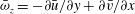 $\bar{\unicode[STIX]{x1D714}}_{z}=-\unicode[STIX]{x2202}\bar{u}/\unicode[STIX]{x2202}y+\unicode[STIX]{x2202}\bar{v}/\unicode[STIX]{x2202}x$
at probe locations, from left to right column,
$\bar{\unicode[STIX]{x1D714}}_{z}=-\unicode[STIX]{x2202}\bar{u}/\unicode[STIX]{x2202}y+\unicode[STIX]{x2202}\bar{v}/\unicode[STIX]{x2202}x$
at probe locations, from left to right column,
 $P1(3.0,0.5),P2(2.0,0.5)$
and close to the centre of the recirculation zone
$P1(3.0,0.5),P2(2.0,0.5)$
and close to the centre of the recirculation zone
 $P3(1.0,0.0)$
.
$P3(1.0,0.0)$
.

4.1.1 Unsteadiness on the three airfoils as a function of
$Re$
and
$AoA$


The onset of flow unsteadiness has been investigated for each of the three profiles in the ranges
 $150\leqslant Re\leqslant 300$
and
$150\leqslant Re\leqslant 300$
and
 $10^{\circ }\leqslant AoA\leqslant 20^{\circ }$
, within which massive separation and unsteadiness are expected. Table 3 presents a qualitative description of the state of the flow. On all airfoils, an increase of
$10^{\circ }\leqslant AoA\leqslant 20^{\circ }$
, within which massive separation and unsteadiness are expected. Table 3 presents a qualitative description of the state of the flow. On all airfoils, an increase of
 $Re$
or
$Re$
or
 $AoA$
promotes unsteadiness and a time-periodic flow is set up, the period of which will be characterized in § 4.4. At a given Reynolds number and low angle of attack, thickness promotes unsteadiness, as seen at
$AoA$
promotes unsteadiness and a time-periodic flow is set up, the period of which will be characterized in § 4.4. At a given Reynolds number and low angle of attack, thickness promotes unsteadiness, as seen at
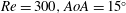 $Re=300,AoA=15^{\circ }$
for the NACA 0009 and 0015 airfoils. Close to stall, camber of the airfoil also promotes unsteadiness, as seen at
$Re=300,AoA=15^{\circ }$
for the NACA 0009 and 0015 airfoils. Close to stall, camber of the airfoil also promotes unsteadiness, as seen at
 $Re=220,AoA=18^{\circ }$
, where flow around the NACA 0015 is still steady while that in the wake of the NACA 4415 airfoil is time periodic.
$Re=220,AoA=18^{\circ }$
, where flow around the NACA 0015 is still steady while that in the wake of the NACA 4415 airfoil is time periodic.
Table 3. Unsteadiness as a function of
 $Re$
and
$Re$
and
 $AoA$
for three NACA airfoils. S: steady, Us: unsteady base flow.
$AoA$
for three NACA airfoils. S: steady, Us: unsteady base flow.

In view of the association of the level of recirculation in the nominally stationary laminar separation bubble (LSB) of the base flow with the appearance of absolute/global linear instability (Allen & Riley Reference Allen and Riley1995; Hammond & Redekopp Reference Hammond and Redekopp1998; Rist & Maucher Reference Rist and Maucher2002; Abdessemed et al.
Reference Abdessemed, Sherwin and Theofilis2009b
; Embacher & Fasel Reference Embacher and Fasel2014) the results of table 3 are quantified in table 4 in terms of the percentage of flow recirculation in the LSB. It is seen that in all airfoils an increase in
 $Re$
or in
$Re$
or in
 $AoA$
leads to an increased maximum recirculation level. At the same
$AoA$
leads to an increased maximum recirculation level. At the same
 $Re$
and
$Re$
and
 $AoA$
values, an increase in either airfoil thickness or camber also increases the level of recirculating flow. It is also noted that in most cases shown recirculation is less than the value of 7.5 % found by Rodríguez & Theofilis (Reference Rodríguez and Theofilis2010) to be necessary for amplification of the stationary three-dimensional global mode in the LSB created by an adverse pressure gradient on a flat plate; further discussion of this point will be provided in the next section.
$AoA$
values, an increase in either airfoil thickness or camber also increases the level of recirculating flow. It is also noted that in most cases shown recirculation is less than the value of 7.5 % found by Rodríguez & Theofilis (Reference Rodríguez and Theofilis2010) to be necessary for amplification of the stationary three-dimensional global mode in the LSB created by an adverse pressure gradient on a flat plate; further discussion of this point will be provided in the next section.
Table 4. Maximum recirculation,
 $|\bar{u}_{min}/\bar{u}_{max}\times 100|$
as a function of
$|\bar{u}_{min}/\bar{u}_{max}\times 100|$
as a function of
 $Re$
and
$Re$
and
 $AoA$
.
$AoA$
.

4.2 Modal stability analysis: solution of the eigenvalue problem
Results of modal instability analysis of flow around the three airfoils at selected combinations of the Reynolds number and angle of attack parameters shown in tables 3 and 4 are discussed in this section. Steady base flows are analysed by solution of the pertinent eigenvalue problem (2.5), whereby the spanwise spatial direction is considered homogeneous and is discretized by a Fourier ansatz, which introduces the wavenumber parameter
 $\unicode[STIX]{x1D6FD}=2\unicode[STIX]{x03C0}/L_{z}$
,
$\unicode[STIX]{x1D6FD}=2\unicode[STIX]{x03C0}/L_{z}$
,
 $L_{z}$
being the spanwise periodicity length, as discussed in § 2. The decomposition decouples the linearized problems to be solved for each
$L_{z}$
being the spanwise periodicity length, as discussed in § 2. The decomposition decouples the linearized problems to be solved for each
 $\unicode[STIX]{x1D6FD}$
from each other, and the full three-dimensional space is covered by varying the wavenumber in a range from
$\unicode[STIX]{x1D6FD}$
from each other, and the full three-dimensional space is covered by varying the wavenumber in a range from
 $\unicode[STIX]{x1D6FD}=0$
, i.e.
$\unicode[STIX]{x1D6FD}=0$
, i.e.
 $L_{z}\rightarrow \infty$
, corresponding to two-dimensional perturbations, to a finite number of discrete
$L_{z}\rightarrow \infty$
, corresponding to two-dimensional perturbations, to a finite number of discrete
 $\unicode[STIX]{x1D6FD}\neq 0$
values corresponding to progressively smaller periodicity lengths, until
$\unicode[STIX]{x1D6FD}\neq 0$
values corresponding to progressively smaller periodicity lengths, until
 $L_{z}=O(1)$
is reached. Modal instability analyses were performed using mesh sizes and spatial polynomial orders comparable to those used for the recovery of the base flow and convergence tests are shown in appendix A.
$L_{z}=O(1)$
is reached. Modal instability analyses were performed using mesh sizes and spatial polynomial orders comparable to those used for the recovery of the base flow and convergence tests are shown in appendix A.
Results have been obtained for all three airfoils, however discussion commences by focusing on the NACA 0015 airfoil at
 $Re=200,AoA=18^{\circ }$
, conditions at which previous analyses have produced contradictory predictions regarding which of the two instability scenarios prevails, namely two-dimensional oscillatory (Brehm & Fasel Reference Brehm and Fasel2011) or three-dimensional stationary (Kitsios et al.
Reference Kitsios, Rodríguez, Theofilis, Ooi and Soria2009; Rodríguez & Theofilis Reference Rodríguez and Theofilis2011). In order to cross-verify predictions, instability results are obtained at these conditions using the time stepping code nektar++ and the matrix-forming code FreeFEM++. The time stepping technique (Barkley et al.
Reference Barkley, Blackburn and Sherwin2008) initializes linear perturbations with a normalized unit vector and evolves them during a non-dimensional time interval of unity, using the same mesh and time step employed for the base flow computations. By contrast, the matrix-forming technique uses a weak formulation of the linearized equations of motion, first to solve for the base flow on a high-density unstructured mesh and subsequently to form the matrix entries corresponding to the eigenvalue problem. Both approaches proceed by constructing Krylov subspaces of orthonormal vectors and an Arnoldi algorithm is used to recover a small number of physically most significant eigenmodes (Theofilis Reference Theofilis2011). The leading two eigenmodes discovered in the wavenumber range
$Re=200,AoA=18^{\circ }$
, conditions at which previous analyses have produced contradictory predictions regarding which of the two instability scenarios prevails, namely two-dimensional oscillatory (Brehm & Fasel Reference Brehm and Fasel2011) or three-dimensional stationary (Kitsios et al.
Reference Kitsios, Rodríguez, Theofilis, Ooi and Soria2009; Rodríguez & Theofilis Reference Rodríguez and Theofilis2011). In order to cross-verify predictions, instability results are obtained at these conditions using the time stepping code nektar++ and the matrix-forming code FreeFEM++. The time stepping technique (Barkley et al.
Reference Barkley, Blackburn and Sherwin2008) initializes linear perturbations with a normalized unit vector and evolves them during a non-dimensional time interval of unity, using the same mesh and time step employed for the base flow computations. By contrast, the matrix-forming technique uses a weak formulation of the linearized equations of motion, first to solve for the base flow on a high-density unstructured mesh and subsequently to form the matrix entries corresponding to the eigenvalue problem. Both approaches proceed by constructing Krylov subspaces of orthonormal vectors and an Arnoldi algorithm is used to recover a small number of physically most significant eigenmodes (Theofilis Reference Theofilis2011). The leading two eigenmodes discovered in the wavenumber range
 $0\leqslant \unicode[STIX]{x1D6FD}\leqslant 10$
by the two approaches are shown in figure 3, from which results obtained using the time stepping code nek5000 are omitted, since they were identical with those produced by the nektar++ code. Analogous results were obtained for the other two airfoils at the same parameters, but are not shown here for brevity.
$0\leqslant \unicode[STIX]{x1D6FD}\leqslant 10$
by the two approaches are shown in figure 3, from which results obtained using the time stepping code nek5000 are omitted, since they were identical with those produced by the nektar++ code. Analogous results were obtained for the other two airfoils at the same parameters, but are not shown here for brevity.

Figure 3. Growth rate and Strouhal number of the least-damped modes of the NACA 0015 airfoil at
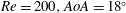 $Re=200,AoA=18^{\circ }$
, obtained by the nektar++ time stepping (open symbol) and the FreeFEM++ matrix-forming (full symbol) methodologies.
$Re=200,AoA=18^{\circ }$
, obtained by the nektar++ time stepping (open symbol) and the FreeFEM++ matrix-forming (full symbol) methodologies.
The agreement between the predictions of the time stepping and the matrix-forming approaches is remarkable, given that the results shown have been obtained using entirely different methodologies, both in terms of theoretical background and in terms of numerical implementation. Despite the quantitative differences in the damping rate results, both methodologies predict the existence of two dominant linear modal perturbations, namely a travelling eigenmode which predominates at relatively small
 $\unicode[STIX]{x1D6FD}$
(large
$\unicode[STIX]{x1D6FD}$
(large
 $L_{z}$
) values and a stationary eigenmode which is less damped than the travelling disturbance at larger
$L_{z}$
) values and a stationary eigenmode which is less damped than the travelling disturbance at larger
 $\unicode[STIX]{x1D6FD}$
(small
$\unicode[STIX]{x1D6FD}$
(small
 $L_{z}$
) values. The cutoff point at which the nature of instability changes at these conditions is found to be
$L_{z}$
) values. The cutoff point at which the nature of instability changes at these conditions is found to be
 $\unicode[STIX]{x1D6FD}\approx 2.5$
.
$\unicode[STIX]{x1D6FD}\approx 2.5$
.
Examination of the spatial structure of the eigenfunctions reveals that these modes correspond to the instabilities known from the earlier analyses of Kitsios et al. (Reference Kitsios, Rodríguez, Theofilis, Ooi and Soria2009) and Rodríguez & Theofilis (Reference Rodríguez and Theofilis2011). Figure 4 presents the amplitude functions of the perturbation velocity components at
 $\unicode[STIX]{x1D6FD}=1$
and
$\unicode[STIX]{x1D6FD}=1$
and
 $\unicode[STIX]{x1D6FD}=3$
, respectively corresponding to a mode akin to Kelvin–Helmholtz instability in the wake of bluff bodies and the NACA 0012 airfoil discussed in the introduction (Theofilis et al.
Reference Theofilis, Barkley and Sherwin2002), while at the higher wavenumber the mode corresponds to the stationary three-dimensional eigenmode of laminar separation bubbles discovered on the flat plate (Theofilis et al.
Reference Theofilis, Hein and Dallmann2000) and in a multitude of massively separated laminar flow configurations (e.g. Barkley, Gomes & Henderson Reference Barkley, Gomes and Henderson2002; Abdessemed et al.
Reference Abdessemed, Sherwin and Theofilis2009b
; Kitsios et al.
Reference Kitsios, Rodríguez, Theofilis, Ooi and Soria2009; Rodríguez & Theofilis Reference Rodríguez and Theofilis2011).
$\unicode[STIX]{x1D6FD}=3$
, respectively corresponding to a mode akin to Kelvin–Helmholtz instability in the wake of bluff bodies and the NACA 0012 airfoil discussed in the introduction (Theofilis et al.
Reference Theofilis, Barkley and Sherwin2002), while at the higher wavenumber the mode corresponds to the stationary three-dimensional eigenmode of laminar separation bubbles discovered on the flat plate (Theofilis et al.
Reference Theofilis, Hein and Dallmann2000) and in a multitude of massively separated laminar flow configurations (e.g. Barkley, Gomes & Henderson Reference Barkley, Gomes and Henderson2002; Abdessemed et al.
Reference Abdessemed, Sherwin and Theofilis2009b
; Kitsios et al.
Reference Kitsios, Rodríguez, Theofilis, Ooi and Soria2009; Rodríguez & Theofilis Reference Rodríguez and Theofilis2011).

Figure 4. NACA 0015 at
 $Re=200,AoA=18^{\circ }$
. Amplitude functions of the least-damped travelling (a) and stationary (b) perturbation velocity components at
$Re=200,AoA=18^{\circ }$
. Amplitude functions of the least-damped travelling (a) and stationary (b) perturbation velocity components at
 $\unicode[STIX]{x1D6FD}=1$
and
$\unicode[STIX]{x1D6FD}=1$
and
 $\unicode[STIX]{x1D6FD}=3$
, respectively. Normalized by the highest velocity component, from blue
$\unicode[STIX]{x1D6FD}=3$
, respectively. Normalized by the highest velocity component, from blue
 $-0.1$
to red 0.1.
$-0.1$
to red 0.1.
However, the present results differ from those reported by Kitsios et al. (Reference Kitsios, Rodríguez, Theofilis, Ooi and Soria2009) and Rodríguez & Theofilis (Reference Rodríguez and Theofilis2011) in two aspects. First, unlike the prediction of linear instability on the NACA 0015 airfoil at
 $Re=200,AoA=18^{\circ }$
in the earlier works, here only stable eigenvalues have been encountered at all
$Re=200,AoA=18^{\circ }$
in the earlier works, here only stable eigenvalues have been encountered at all
 $\unicode[STIX]{x1D6FD}$
values examined. Second, it is found that at
$\unicode[STIX]{x1D6FD}$
values examined. Second, it is found that at
 $\unicode[STIX]{x1D6FD}=1$
the leading flow eigenmode is the unsteady Kelvin–Helmholtz instability and not the stationary three-dimensional mode, as reported in the earlier work. As a matter of fact, the stationary mode did not become unstable in the range of Reynolds numbers examined, as will be discussed shortly. The stationary mode, which was shown by Rodríguez & Theofilis (Reference Rodríguez and Theofilis2011) to give rise to patterns akin to the stall-cells encountered at flight Reynolds numbers, does overtake the travelling instability at higher
$\unicode[STIX]{x1D6FD}=1$
the leading flow eigenmode is the unsteady Kelvin–Helmholtz instability and not the stationary three-dimensional mode, as reported in the earlier work. As a matter of fact, the stationary mode did not become unstable in the range of Reynolds numbers examined, as will be discussed shortly. The stationary mode, which was shown by Rodríguez & Theofilis (Reference Rodríguez and Theofilis2011) to give rise to patterns akin to the stall-cells encountered at flight Reynolds numbers, does overtake the travelling instability at higher
 $\unicode[STIX]{x1D6FD}$
values. This could be related with the appearance of stall-cell patterns in the low Reynolds number simulations of Taira & Colonius (Reference Taira and Colonius2009) on
$\unicode[STIX]{x1D6FD}$
values. This could be related with the appearance of stall-cell patterns in the low Reynolds number simulations of Taira & Colonius (Reference Taira and Colonius2009) on
 $O(1)$
aspect-ratio wings. However, it is unclear whether results of instability analysis on finite-span wings in that work can be related with those obtained on the present spanwise-periodic geometries. It is also worth noting, that the numerical integrity of the results previously reported by Kitsios et al. (Reference Kitsios, Rodríguez, Theofilis, Ooi and Soria2009) and Rodríguez & Theofilis (Reference Rodríguez and Theofilis2011) was already questioned by Kitsios (Reference Kitsios2010), who reported that the instability analyses presented had not entirely converged. Work is currently underway in order to identify the origin of the discrepancy with the results reported in the earlier analyses.
$O(1)$
aspect-ratio wings. However, it is unclear whether results of instability analysis on finite-span wings in that work can be related with those obtained on the present spanwise-periodic geometries. It is also worth noting, that the numerical integrity of the results previously reported by Kitsios et al. (Reference Kitsios, Rodríguez, Theofilis, Ooi and Soria2009) and Rodríguez & Theofilis (Reference Rodríguez and Theofilis2011) was already questioned by Kitsios (Reference Kitsios2010), who reported that the instability analyses presented had not entirely converged. Work is currently underway in order to identify the origin of the discrepancy with the results reported in the earlier analyses.
Attention is next turned to the dependence of the eigenvalues on the Reynolds number, keeping a constant value of
 $AoA=18^{\circ }$
. Figure 5 shows results for the three airfoils in the range
$AoA=18^{\circ }$
. Figure 5 shows results for the three airfoils in the range
 $150\leqslant Re\leqslant 230$
. In this and all subsequent figures results for the 0009, 0015 and 4415 airfoils will be presented using the circle, ○, square,
$150\leqslant Re\leqslant 230$
. In this and all subsequent figures results for the 0009, 0015 and 4415 airfoils will be presented using the circle, ○, square,
 $\Box$
and diamond, ♢ symbols, respectively. At all
$\Box$
and diamond, ♢ symbols, respectively. At all
 $Re$
values examined in the range
$Re$
values examined in the range
 $0\leqslant \unicode[STIX]{x1D6FD}\leqslant 5$
, the least-damped eigenmode corresponds to the Kelvin–Helmholtz instability, while the stationary three-dimensional eigenmode is substantially more damped. On all three airfoils Kelvin–Helmholtz instability in the wake is the strongest at
$0\leqslant \unicode[STIX]{x1D6FD}\leqslant 5$
, the least-damped eigenmode corresponds to the Kelvin–Helmholtz instability, while the stationary three-dimensional eigenmode is substantially more damped. On all three airfoils Kelvin–Helmholtz instability in the wake is the strongest at
 $\unicode[STIX]{x1D6FD}=0$
and more damped at
$\unicode[STIX]{x1D6FD}=0$
and more damped at
 $\unicode[STIX]{x1D6FD}>0$
. It is the strongest of the two instabilities until
$\unicode[STIX]{x1D6FD}>0$
. It is the strongest of the two instabilities until
 $\unicode[STIX]{x1D6FD}\approx 2.5$
. Beyond this wavenumber the three-dimensional stationary global mode is the dominant instability, albeit damped at all combinations of the
$\unicode[STIX]{x1D6FD}\approx 2.5$
. Beyond this wavenumber the three-dimensional stationary global mode is the dominant instability, albeit damped at all combinations of the
 $(Re,AoA)$
parameters examined. At
$(Re,AoA)$
parameters examined. At
 $\unicode[STIX]{x1D6FD}=0$
the instability analysis results shown are in agreement with the threshold of unsteadiness obtained through two-dimensional numerical simulations of flow around the airfoils. Instability analyses performed at
$\unicode[STIX]{x1D6FD}=0$
the instability analysis results shown are in agreement with the threshold of unsteadiness obtained through two-dimensional numerical simulations of flow around the airfoils. Instability analyses performed at
 $\unicode[STIX]{x1D6FD}\neq 0$
show that the Reynolds number has a quantitative but not a qualitative influence on the relative importance of the three-dimensional wake and stationary eigenmodes. Two sets of results, one at a lower and one at a higher Reynolds number are shown on the 0009 and 4415 airfoils and three such analyses are shown for the 0015 airfoil. As expected, increasing the Reynolds number leads to less stable flow, but does not change the qualitative picture described above, the Kelvin–Helmholtz mode being always less damped than the stationary eigenmode. The first unstable (Kelvin–Helmholtz) mode on the 0015 airfoil is found at
$\unicode[STIX]{x1D6FD}\neq 0$
show that the Reynolds number has a quantitative but not a qualitative influence on the relative importance of the three-dimensional wake and stationary eigenmodes. Two sets of results, one at a lower and one at a higher Reynolds number are shown on the 0009 and 4415 airfoils and three such analyses are shown for the 0015 airfoil. As expected, increasing the Reynolds number leads to less stable flow, but does not change the qualitative picture described above, the Kelvin–Helmholtz mode being always less damped than the stationary eigenmode. The first unstable (Kelvin–Helmholtz) mode on the 0015 airfoil is found at
 $Re=230$
. Figure 5 also documents the effect of Reynolds number on the frequency of the Kelvin–Helmholtz mode on all three airfoils within the
$Re=230$
. Figure 5 also documents the effect of Reynolds number on the frequency of the Kelvin–Helmholtz mode on all three airfoils within the
 $\unicode[STIX]{x1D6FD}$
range in which the Kelvin–Helmholtz is the dominant flow instability. It can be seen that the frequency on each airfoil is practically independent of
$\unicode[STIX]{x1D6FD}$
range in which the Kelvin–Helmholtz is the dominant flow instability. It can be seen that the frequency on each airfoil is practically independent of
 $Re$
and only a weak function of
$Re$
and only a weak function of
 $\unicode[STIX]{x1D6FD}$
, decaying slightly as the wavenumber increases and the corresponding periodicity length shortens.
$\unicode[STIX]{x1D6FD}$
, decaying slightly as the wavenumber increases and the corresponding periodicity length shortens.

Figure 5. Stability analysis of flow around the three airfoils at
 $AoA=18^{\circ }$
. (a) Growth rate of the leading eigenvalue, as function of spanwise wavenumber
$AoA=18^{\circ }$
. (a) Growth rate of the leading eigenvalue, as function of spanwise wavenumber
 $\unicode[STIX]{x1D6FD}$
. (b) Strouhal number dependence on wavenumber. ○: 0009 at
$\unicode[STIX]{x1D6FD}$
. (b) Strouhal number dependence on wavenumber. ○: 0009 at
 $Re=200$
and 220; ▫: 0015 at
$Re=200$
and 220; ▫: 0015 at
 $Re=200$
and 230; ♢: 4415 at
$Re=200$
and 230; ♢: 4415 at
 $Re=150$
and 200. The respective lower
$Re=150$
and 200. The respective lower
 $Re$
value results are denoted by open symbols, while those at the respective higher
$Re$
value results are denoted by open symbols, while those at the respective higher
 $Re$
value are presented by full symbols.
$Re$
value are presented by full symbols.

Figure 6. Stability analysis of flow around the three airfoils at
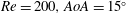 $Re=200,AoA=15^{\circ }$
(open symbols) and
$Re=200,AoA=15^{\circ }$
(open symbols) and
 $18^{\circ }$
(full symbols). (a) Growth rate of the leading eigenvalue, as function of spanwise wavenumber
$18^{\circ }$
(full symbols). (a) Growth rate of the leading eigenvalue, as function of spanwise wavenumber
 $\unicode[STIX]{x1D6FD}$
. (b) Strouhal number dependence on wavenumber. ○: 0009; ▫: 0015; ♢: 4415.
$\unicode[STIX]{x1D6FD}$
. (b) Strouhal number dependence on wavenumber. ○: 0009; ▫: 0015; ♢: 4415.
Figure 6 shows the effect on the global eigenmodes of changing the angle of attack while keeping a constant value of
 $Re=200$
. Results obtained at the value of
$Re=200$
. Results obtained at the value of
 $AoA=18^{\circ }$
previously examined, as well as those at a lower value
$AoA=18^{\circ }$
previously examined, as well as those at a lower value
 $AoA=15^{\circ }$
are shown, since angles of attack beyond the higher of the two lead to time-periodic flow. It can be seen that lowering the angle of attack strongly damps both the Kelvin–Helmholtz and the three-dimensional stationary mode on all three airfoils, although the relative importance of the two mechanisms remains the same. It can be anticipated that in the limit of even lower
$AoA=15^{\circ }$
are shown, since angles of attack beyond the higher of the two lead to time-periodic flow. It can be seen that lowering the angle of attack strongly damps both the Kelvin–Helmholtz and the three-dimensional stationary mode on all three airfoils, although the relative importance of the two mechanisms remains the same. It can be anticipated that in the limit of even lower
 $AoA$
values, the Kelvin–Helmholtz instability found by global analysis on the 0012 airfoil (Theofilis et al.
Reference Theofilis, Barkley and Sherwin2002) will also be present on the airfoils considered presently and will also be damped at this low Reynolds number value. It can further be anticipated that, in the limit of lower
$AoA$
values, the Kelvin–Helmholtz instability found by global analysis on the 0012 airfoil (Theofilis et al.
Reference Theofilis, Barkley and Sherwin2002) will also be present on the airfoils considered presently and will also be damped at this low Reynolds number value. It can further be anticipated that, in the limit of lower
 $AoA$
values Tollmien–Schlichting instabilities in the boundary layer around the airfoil will emerge in the eigenspectrum. However, the Reynolds number range examined is too low for such an instability to be active.
$AoA$
values Tollmien–Schlichting instabilities in the boundary layer around the airfoil will emerge in the eigenspectrum. However, the Reynolds number range examined is too low for such an instability to be active.
With regards to the three-dimensional stationary mode of laminar separation, it has been found to be damped on all three airfoils at all parameters examined, despite the existence of certain combinations of the
 $(Re,AoA)$
parameters at which the level of recirculation in the primary separation bubble exceeds the value of 7.5 %, predicted by Rodríguez & Theofilis (Reference Rodríguez and Theofilis2010) to be sufficient for this mode to be amplified on the flat plate. Present results suggest that higher levels of recirculation are required for instability of the stationary mode of laminar separation on any of the three airfoils analysed.
$(Re,AoA)$
parameters at which the level of recirculation in the primary separation bubble exceeds the value of 7.5 %, predicted by Rodríguez & Theofilis (Reference Rodríguez and Theofilis2010) to be sufficient for this mode to be amplified on the flat plate. Present results suggest that higher levels of recirculation are required for instability of the stationary mode of laminar separation on any of the three airfoils analysed.
The effect of thickness and camber on the characteristics of the eigenmodes discussed can be examined by reference to a set of parameters,
 $Re=200,AoA=18^{\circ }$
, at which results have been obtained for all three airfoils. It can be seen in figures 5 and 6 that thickness and camber introduce quantitative but not qualitative differences to the instability results. Increasing thickness in the symmetric airfoils while maintaining the same (zero) camber, results in a flow that is less stable against both Kelvin–Helmholtz and three-dimensional stationary modes. The same effect is found by an increase in camber while the airfoil thickness is maintained, namely a destabilization of both classes of global instabilities.
$Re=200,AoA=18^{\circ }$
, at which results have been obtained for all three airfoils. It can be seen in figures 5 and 6 that thickness and camber introduce quantitative but not qualitative differences to the instability results. Increasing thickness in the symmetric airfoils while maintaining the same (zero) camber, results in a flow that is less stable against both Kelvin–Helmholtz and three-dimensional stationary modes. The same effect is found by an increase in camber while the airfoil thickness is maintained, namely a destabilization of both classes of global instabilities.
4.3 Non-modal linear stability analysis
Linear stability analysis of steady base flows is completed in this section by studying the short-time evolution of small-amplitude three-dimensional perturbations superposed upon the two-dimensional base flows over the three NACA airfoils. Ample evidence can be found in the literature that substantial transient energy growth can be expected on both bluff bodies (Abdessemed et al.
Reference Abdessemed, Sharma, Sherwin and Theofilis2009a
) and lifting surfaces (Abdessemed et al.
Reference Abdessemed, Sherwin and Theofilis2009b
), while first non-modal stability analysis results of flow around airfoils at large angles of attack have also been obtained recently (Gioria et al.
Reference Gioria, He and Theofilis2014; Loh et al.
Reference Loh, Blackburn and Sherwin2014; Gioria et al.
Reference Gioria, He and Theofilis2015). The steady base flows shown in tables 3 and 4 are analysed with respect to their capacity to sustain transient energy growth at Reynolds numbers slightly below the primary transition to a periodic wake. For the analysis that follows the choice of range of spanwise wavenumbers monitored,
 $0\leqslant \unicode[STIX]{x1D6FD}\leqslant 2\unicode[STIX]{x03C0}$
, was based on results of Gioria et al. (Reference Gioria, He and Theofilis2015) and the direct-adjoint iteration procedure (Barkley et al.
Reference Barkley, Blackburn and Sherwin2008) is performed for time horizons
$0\leqslant \unicode[STIX]{x1D6FD}\leqslant 2\unicode[STIX]{x03C0}$
, was based on results of Gioria et al. (Reference Gioria, He and Theofilis2015) and the direct-adjoint iteration procedure (Barkley et al.
Reference Barkley, Blackburn and Sherwin2008) is performed for time horizons
 $\unicode[STIX]{x1D70F}$
long enough for the maximum of the gain function
$\unicode[STIX]{x1D70F}$
long enough for the maximum of the gain function
 $G(\unicode[STIX]{x1D70F})$
to be well defined at all spanwise wavenumbers
$G(\unicode[STIX]{x1D70F})$
to be well defined at all spanwise wavenumbers
 $\unicode[STIX]{x1D6FD}$
.
$\unicode[STIX]{x1D6FD}$
.
Figure 7 presents
 $G(\unicode[STIX]{x1D70F})$
results at spanwise wavenumber values
$G(\unicode[STIX]{x1D70F})$
results at spanwise wavenumber values
 $0\leqslant \unicode[STIX]{x1D6FD}\leqslant 2\unicode[STIX]{x03C0}$
for all three profiles. Higher
$0\leqslant \unicode[STIX]{x1D6FD}\leqslant 2\unicode[STIX]{x03C0}$
for all three profiles. Higher
 $\unicode[STIX]{x1D6FD}$
values were not analysed, since it is clear from the results shown that the largest transient energy growth is attained for two-dimensional perturbations (
$\unicode[STIX]{x1D6FD}$
values were not analysed, since it is clear from the results shown that the largest transient energy growth is attained for two-dimensional perturbations (
 $\unicode[STIX]{x1D6FD}=0$
). The results are qualitatively similar on all three airfoils and, in turn, analogous to those obtained on the circular cylinder (Abdessemed et al.
Reference Abdessemed, Sharma, Sherwin and Theofilis2009a
). Interestingly, flow corresponding to the smaller wavenumber values shown in the results on all three airfoils also exhibits relatively large transient growth, implying that low Reynolds number flow around large aspect ratio untapered and unswept wings may experience this linear instability mechanism if placed at high angles of attack to the oncoming flow. It should be noted that the
$\unicode[STIX]{x1D6FD}=0$
). The results are qualitatively similar on all three airfoils and, in turn, analogous to those obtained on the circular cylinder (Abdessemed et al.
Reference Abdessemed, Sharma, Sherwin and Theofilis2009a
). Interestingly, flow corresponding to the smaller wavenumber values shown in the results on all three airfoils also exhibits relatively large transient growth, implying that low Reynolds number flow around large aspect ratio untapered and unswept wings may experience this linear instability mechanism if placed at high angles of attack to the oncoming flow. It should be noted that the
 $\unicode[STIX]{x1D6FD}=0$
instability only overtakes its three-dimensional counterparts after a certain time has elapsed; this result can be seen in figure 8 and points to the fact that an appropriate range of time needs to be evaluated in the analysis, in order to establish which class of perturbations grows at most transiently. The times monitored presently point to three-dimensional effects being more relevant for time scales of
$\unicode[STIX]{x1D6FD}=0$
instability only overtakes its three-dimensional counterparts after a certain time has elapsed; this result can be seen in figure 8 and points to the fact that an appropriate range of time needs to be evaluated in the analysis, in order to establish which class of perturbations grows at most transiently. The times monitored presently point to three-dimensional effects being more relevant for time scales of
 $O(1)$
, corresponding to the advection time for a linear perturbation to travel the length of the airfoil chord, while the largest transient growth is attained through the Orr mechanism by two-dimensional perturbations, as they deform while being advected downstream along the wake.
$O(1)$
, corresponding to the advection time for a linear perturbation to travel the length of the airfoil chord, while the largest transient growth is attained through the Orr mechanism by two-dimensional perturbations, as they deform while being advected downstream along the wake.

Figure 7. Optimal gain
 $G(\unicode[STIX]{x1D70F})$
as a function of wavenumber
$G(\unicode[STIX]{x1D70F})$
as a function of wavenumber
 $\unicode[STIX]{x1D6FD}$
at
$\unicode[STIX]{x1D6FD}$
at
 $Re=200,AoA=18^{\circ }$
for the 0009 (○), 0015 (▫) and 4415 (♢) airfoils. Upper to lower curves:
$Re=200,AoA=18^{\circ }$
for the 0009 (○), 0015 (▫) and 4415 (♢) airfoils. Upper to lower curves:
 $\unicode[STIX]{x1D6FD}=0,\unicode[STIX]{x03C0}/8,\unicode[STIX]{x03C0}/4,\unicode[STIX]{x03C0}/2,\unicode[STIX]{x03C0}$
and
$\unicode[STIX]{x1D6FD}=0,\unicode[STIX]{x03C0}/8,\unicode[STIX]{x03C0}/4,\unicode[STIX]{x03C0}/2,\unicode[STIX]{x03C0}$
and
 $2\unicode[STIX]{x03C0}$
.
$2\unicode[STIX]{x03C0}$
.

Figure 8. Maximum gain,
 $G(\unicode[STIX]{x1D70F})$
at
$G(\unicode[STIX]{x1D70F})$
at
 $\unicode[STIX]{x1D6FD}=0$
(solid line),
$\unicode[STIX]{x1D6FD}=0$
(solid line),
 $\unicode[STIX]{x1D6FD}=\unicode[STIX]{x03C0}/4$
(– – –),
$\unicode[STIX]{x1D6FD}=\unicode[STIX]{x03C0}/4$
(– – –),
 $\unicode[STIX]{x1D6FD}=\unicode[STIX]{x03C0}/2$
(— ⋅ —) and
$\unicode[STIX]{x1D6FD}=\unicode[STIX]{x03C0}/2$
(— ⋅ —) and
 $\unicode[STIX]{x1D6FD}=\unicode[STIX]{x03C0}$
(
$\unicode[STIX]{x1D6FD}=\unicode[STIX]{x03C0}$
(
 $\cdots \cdots$
) for the 0015 airfoil at
$\cdots \cdots$
) for the 0015 airfoil at
 $Re=200,AoA=18^{\circ }$
at short time horizons in the range
$Re=200,AoA=18^{\circ }$
at short time horizons in the range
 $0\leqslant \unicode[STIX]{x1D70F}\leqslant 4$
.
$0\leqslant \unicode[STIX]{x1D70F}\leqslant 4$
.
At asymptotically large times, time integration of the linearized system of perturbations, as done in non-modal analysis, is expected to deliver the least-damped eigenmode results that modal theory delivers through solution of the eigenvalue problem. Figure 9 presents the initial optimal perturbation in terms of its three velocity components in the top row, followed by optimal linear perturbations at different, progressively larger time horizons
 $\unicode[STIX]{x1D70F}$
. The optimal initial conditions are strongly reminiscent of those found on the low pressure turbine (LPT) cascade analysis (Abdessemed et al.
Reference Abdessemed, Sherwin and Theofilis2009b
, figure 17) where structures inclined against the main shear were also observed. As time progresses, the perturbations evolve into the amplitude functions of the Kelvin–Helmholtz modal instability in the wake, shown in figure 4.
$\unicode[STIX]{x1D70F}$
. The optimal initial conditions are strongly reminiscent of those found on the low pressure turbine (LPT) cascade analysis (Abdessemed et al.
Reference Abdessemed, Sherwin and Theofilis2009b
, figure 17) where structures inclined against the main shear were also observed. As time progresses, the perturbations evolve into the amplitude functions of the Kelvin–Helmholtz modal instability in the wake, shown in figure 4.

Figure 9. Optimal perturbations of the flow past the NACA 0015 airfoil at
 $Re=200,AoA=18^{\circ },\unicode[STIX]{x1D6FD}=1$
. From (a–g),
$Re=200,AoA=18^{\circ },\unicode[STIX]{x1D6FD}=1$
. From (a–g),
 $\unicode[STIX]{x1D70F}=0,10,20,30,40,50$
and 60.
$\unicode[STIX]{x1D70F}=0,10,20,30,40,50$
and 60.
The dependence of the optimal gain on parameter changes is documented in figure 10. Figure 10(a,c,e) presents results of changes in Reynolds number at a fixed
 $AoA=18^{\circ }$
. Results at
$AoA=18^{\circ }$
. Results at
 $Re=150$
and
$Re=150$
and
 $200$
are shown for all three airfoils and, in addition, those at
$200$
are shown for all three airfoils and, in addition, those at
 $Re=220$
, at which the base flow is still steady, are presented for the 0009 and 0015 airfoils. Figure 10(b,d,f) shows the effect on
$Re=220$
, at which the base flow is still steady, are presented for the 0009 and 0015 airfoils. Figure 10(b,d,f) shows the effect on
 $G(\unicode[STIX]{x1D70F})$
of keeping
$G(\unicode[STIX]{x1D70F})$
of keeping
 $Re=200$
constant and varying the angle of attack parameter at the values
$Re=200$
constant and varying the angle of attack parameter at the values
 $AoA=10^{\circ },15^{\circ }$
and
$AoA=10^{\circ },15^{\circ }$
and
 $18^{\circ }$
. It can be seen that changes of
$18^{\circ }$
. It can be seen that changes of
 $O(20\,\%)$
in either parameter lead to up to three orders of magnitude increase of the maximum value of
$O(20\,\%)$
in either parameter lead to up to three orders of magnitude increase of the maximum value of
 $G(\unicode[STIX]{x1D70F})$
. This is consistent with the
$G(\unicode[STIX]{x1D70F})$
. This is consistent with the
 $G\sim O(10^{10})$
prediction of Loh et al. (Reference Loh, Blackburn and Sherwin2014) on the NACA 0012 airfoil at separated flow conditions, and analogously large gains found in other flows exhibiting large-scale laminar separation (e.g. Blackburn, Barkley & Sherwin Reference Blackburn, Barkley and Sherwin2008a
; Blackburn, Sherwin & Barkley Reference Blackburn, Sherwin and Barkley2008b
). Such large transient energy amplification values are also known from the related earlier works of Abdessemed et al. (Reference Abdessemed, Sherwin and Theofilis2009b
) and Sharma et al. (Reference Sharma, Abdessemed, Sherwin and Theofilis2011) in the wake of an LPT blade cascade, as well as from the analogous analysis of Abdessemed et al. (Reference Abdessemed, Sharma, Sherwin and Theofilis2009a
) in the circular cylinder wake. While the relevance of the strong transient growth in the LPT cascade to the present open flow results may be questioned on account of the transverse periodicity of the domain analysed, the results of figures 7 and 10 are entirely consistent with those in the wake of the cylinder: two-dimensional perturbations experience the strongest transient growth, while the relevance of this scenario is diminishing for increasingly large wavenumbers/short spanwise domain lengths.
$G\sim O(10^{10})$
prediction of Loh et al. (Reference Loh, Blackburn and Sherwin2014) on the NACA 0012 airfoil at separated flow conditions, and analogously large gains found in other flows exhibiting large-scale laminar separation (e.g. Blackburn, Barkley & Sherwin Reference Blackburn, Barkley and Sherwin2008a
; Blackburn, Sherwin & Barkley Reference Blackburn, Sherwin and Barkley2008b
). Such large transient energy amplification values are also known from the related earlier works of Abdessemed et al. (Reference Abdessemed, Sherwin and Theofilis2009b
) and Sharma et al. (Reference Sharma, Abdessemed, Sherwin and Theofilis2011) in the wake of an LPT blade cascade, as well as from the analogous analysis of Abdessemed et al. (Reference Abdessemed, Sharma, Sherwin and Theofilis2009a
) in the circular cylinder wake. While the relevance of the strong transient growth in the LPT cascade to the present open flow results may be questioned on account of the transverse periodicity of the domain analysed, the results of figures 7 and 10 are entirely consistent with those in the wake of the cylinder: two-dimensional perturbations experience the strongest transient growth, while the relevance of this scenario is diminishing for increasingly large wavenumbers/short spanwise domain lengths.

Figure 10. Maximum gain,
 $G(\unicode[STIX]{x1D70F})$
at
$G(\unicode[STIX]{x1D70F})$
at
 $\unicode[STIX]{x1D6FD}=0$
for the 0009 (○), 0015 (▫) and 4415 (♢) airfoils. (a,c,e) Effect of Reynolds number,
$\unicode[STIX]{x1D6FD}=0$
for the 0009 (○), 0015 (▫) and 4415 (♢) airfoils. (a,c,e) Effect of Reynolds number,
 $Re=150,200$
and 220 at
$Re=150,200$
and 220 at
 $AoA=18^{\circ }$
. (b,d,f) Effect of angle of attack,
$AoA=18^{\circ }$
. (b,d,f) Effect of angle of attack,
 $AoA=10^{\circ },15^{\circ }$
and
$AoA=10^{\circ },15^{\circ }$
and
 $18^{\circ }$
at
$18^{\circ }$
at
 $Re=200$
.
$Re=200$
.
Finally, figure 11 compares the maximum transient growth on the three airfoils at the respective optimal conditions. It can be seen that an increase in airfoil thickness for the two symmetric airfoils, as well as an increase in camber for the two thicker airfoils leads to increase in the maximal gain obtained. This result could be significant for applications such as wind turbine blades, in which airfoils substantially thicker than the ones examined presently are utilized.

Figure 11. Optimal gain at
 $Re=200,AoA=18^{\circ },\unicode[STIX]{x1D6FD}=0$
for the 0009 (○), 0015 (▫) and 4415 (♢) airfoils as a function of airfoil thickness and camber.
$Re=200,AoA=18^{\circ },\unicode[STIX]{x1D6FD}=0$
for the 0009 (○), 0015 (▫) and 4415 (♢) airfoils as a function of airfoil thickness and camber.
4.4 Instability analysis of periodic wakes on the three NACA airfoils
Time-periodic base flows were obtained by running two-dimensional laminar direct numerical simulations for sufficient time until well-defined periodic signals were obtained. The temporal dependence of integral quantities, such as the forces exerted on the airfoil surface, reached a periodic behaviour with a given frequency and its harmonics, while probes at random locations in the wake identified the (same) frequencies and (different) amplitudes related to the passage of vortices related with the periodic shedding at the leading and trailing edge. The non-dimensional Strouhal number,
 $St$
, associated with the shedding frequency of the periodic wave that arises from the first bifurcation examined in § 4.2, is shown in figure 12 in the range of Reynolds numbers considered in this study. Error bars are added to the results, reflecting the different methods used to estimate the signal frequency from the simulation results. The same pattern emerges for all three airfoils, namely that an increase of
$St$
, associated with the shedding frequency of the periodic wave that arises from the first bifurcation examined in § 4.2, is shown in figure 12 in the range of Reynolds numbers considered in this study. Error bars are added to the results, reflecting the different methods used to estimate the signal frequency from the simulation results. The same pattern emerges for all three airfoils, namely that an increase of
 $Re$
leads to almost quadratic increase of the perturbation frequency at the lower Reynolds numbers, while a trend of
$Re$
leads to almost quadratic increase of the perturbation frequency at the lower Reynolds numbers, while a trend of
 $St$
to saturate is observed at the highest
$St$
to saturate is observed at the highest
 $Re$
-values examined. Moreover, thickness and camber of the airfoil do not appear to have a strong influence on the
$Re$
-values examined. Moreover, thickness and camber of the airfoil do not appear to have a strong influence on the
 $St$
values obtained at each Reynolds number, although a steeper increase can be seen in the curve corresponding to the cambered airfoil compared to its symmetric counterparts.
$St$
values obtained at each Reynolds number, although a steeper increase can be seen in the curve corresponding to the cambered airfoil compared to its symmetric counterparts.

Figure 12. Dependence of the Strouhal number of the wake behind the 0009 (○), 0015 (▫) and 4415 (♢) airfoils as function on the Reynolds number considered in this work.
Thirty two snapshots are obtained from the periodic base flow in one period and are interpolated spectrally from the full domain onto a domain of smaller extent around the airfoil. The resulting high-resolution interpolated snapshots are then used in the subsequent linear temporal Floquet instability analysis, in which the wavenumber corresponding to the spanwise direction is fixed. The inflow and far-field boundary conditions on all perturbations are homogeneous Dirichlet for the velocity and homogeneous high-order boundary conditions for the pressure, while the outflow boundary conditions for velocity and pressure perturbations are homogeneous Neumann and homogeneous Dirichlet boundary conditions, respectively. The action of the linear operator over the amplitude function of the perturbations in the resolution of the Floquet analysis is obtained by direct integration of the linearized version of the Navier–Stokes equations.
The secondary instability arising when the time-periodic flow becomes unstable to three-dimensional perturbations is considered by examining the dependence of the modulus of the Floquet multipliers,
 $\unicode[STIX]{x1D707}$
, on the flow parameters
$\unicode[STIX]{x1D707}$
, on the flow parameters
 $Re$
and
$Re$
and
 $AoA$
, as well as on the geometric parameters of airfoil thickness and camber. Monitored are high values of the angle of attack and Reynolds numbers past the two-dimensional Hopf bifurcation, until two distinct three-dimensional perturbations have become unstable. Figure 13 presents the dependence of the modulus of the Floquet multiplier
$AoA$
, as well as on the geometric parameters of airfoil thickness and camber. Monitored are high values of the angle of attack and Reynolds numbers past the two-dimensional Hopf bifurcation, until two distinct three-dimensional perturbations have become unstable. Figure 13 presents the dependence of the modulus of the Floquet multiplier
 $\unicode[STIX]{x1D707}$
on the spanwise wavenumber
$\unicode[STIX]{x1D707}$
on the spanwise wavenumber
 $\unicode[STIX]{x1D6FD}$
for the three airfoils in the Reynolds number range
$\unicode[STIX]{x1D6FD}$
for the three airfoils in the Reynolds number range
 $400\leqslant Re\leqslant 600$
at
$400\leqslant Re\leqslant 600$
at
 $AoA=20^{\circ }$
. Starting from two-dimensional flow,
$AoA=20^{\circ }$
. Starting from two-dimensional flow,
 $\unicode[STIX]{x1D6FD}=0$
, discrete values of the spanwise wavenumber parameter are examined until linear three-dimensional instability is encountered in the examined wavenumber range
$\unicode[STIX]{x1D6FD}=0$
, discrete values of the spanwise wavenumber parameter are examined until linear three-dimensional instability is encountered in the examined wavenumber range
 $0\leqslant \unicode[STIX]{x1D6FD}\leqslant 20$
. Any three-dimensional instability is expected to be encountered in this range, since at high
$0\leqslant \unicode[STIX]{x1D6FD}\leqslant 20$
. Any three-dimensional instability is expected to be encountered in this range, since at high
 $\unicode[STIX]{x1D6FD}$
numbers the solution is dominated by viscous effects, for which multipliers are negative and proportional to
$\unicode[STIX]{x1D6FD}$
numbers the solution is dominated by viscous effects, for which multipliers are negative and proportional to
 $\text{e}^{-\unicode[STIX]{x1D6FD}^{2}}$
. It should be noted that the zero crossing of the Floquet multiplier in the vicinity of
$\text{e}^{-\unicode[STIX]{x1D6FD}^{2}}$
. It should be noted that the zero crossing of the Floquet multiplier in the vicinity of
 $\unicode[STIX]{x1D6FD}\rightarrow 0$
in the results of the NACA 0009 airfoil is a numerical artefact introduced by the increasingly stiff nature of the eigenvalue problem in this limit and should not be interpreted as a physical instability.
$\unicode[STIX]{x1D6FD}\rightarrow 0$
in the results of the NACA 0009 airfoil is a numerical artefact introduced by the increasingly stiff nature of the eigenvalue problem in this limit and should not be interpreted as a physical instability.

Figure 13. Maximum Floquet multiplier,
 $\unicode[STIX]{x1D707}$
, as function of wavenumber
$\unicode[STIX]{x1D707}$
, as function of wavenumber
 $\unicode[STIX]{x1D6FD}$
at
$\unicode[STIX]{x1D6FD}$
at
 $AoA=20^{\circ }$
. (a) NACA 0009 at (upper-to-lower)
$AoA=20^{\circ }$
. (a) NACA 0009 at (upper-to-lower)
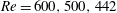 $Re=600,500,442$
and 400. (b) NACA 0015 at (upper-to-lower)
$Re=600,500,442$
and 400. (b) NACA 0015 at (upper-to-lower)
 $Re=600,500,474$
and 400. (c) NACA 4415 at (upper-to-lower)
$Re=600,500,474$
and 400. (c) NACA 4415 at (upper-to-lower)
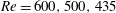 $Re=600,500,435$
and 400.
$Re=600,500,435$
and 400.
Results obtained are qualitatively analogous on all three profiles. At the lowest Reynolds number shown,
 $Re=400$
, all Floquet multipliers remain
$Re=400$
, all Floquet multipliers remain
 $|\unicode[STIX]{x1D707}|<1$
, implying stability of the corresponding periodic orbit: the two-dimensional time-periodic flow examined is also a solution of the three-dimensional equations of motion. Several intermediate Reynolds numbers were examined until the next Reynolds number values shown,
$|\unicode[STIX]{x1D707}|<1$
, implying stability of the corresponding periodic orbit: the two-dimensional time-periodic flow examined is also a solution of the three-dimensional equations of motion. Several intermediate Reynolds numbers were examined until the next Reynolds number values shown,
 $Re\approx 442$
, 474 and 435, for the NACA 0009, 0015 and 4415 profiles, respectively. At these Reynolds number values three-dimensional perturbations with
$Re\approx 442$
, 474 and 435, for the NACA 0009, 0015 and 4415 profiles, respectively. At these Reynolds number values three-dimensional perturbations with
 $\unicode[STIX]{x1D6FD}\approx 11$
reach
$\unicode[STIX]{x1D6FD}\approx 11$
reach
 $\unicode[STIX]{x1D707}\approx 1$
, namely the two-dimensional periodic orbits become unstable to three-dimensional perturbations that are spanwise periodic with a periodicity length of
$\unicode[STIX]{x1D707}\approx 1$
, namely the two-dimensional periodic orbits become unstable to three-dimensional perturbations that are spanwise periodic with a periodicity length of
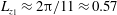 $L_{z_{1}}\approx 2\unicode[STIX]{x03C0}/11\approx 0.57$
chord lengths. The curves in figure 13 where the maximum value of
$L_{z_{1}}\approx 2\unicode[STIX]{x03C0}/11\approx 0.57$
chord lengths. The curves in figure 13 where the maximum value of
 $\unicode[STIX]{x1D707}$
of the short-wavelength modal perturbations is equal to unity correspond with the critical Reynolds number of this secondary flow eigenmode. When the Reynolds number is increased to
$\unicode[STIX]{x1D707}$
of the short-wavelength modal perturbations is equal to unity correspond with the critical Reynolds number of this secondary flow eigenmode. When the Reynolds number is increased to
 $Re=500$
and 600 the instability of the mode peaking around
$Re=500$
and 600 the instability of the mode peaking around
 $\unicode[STIX]{x1D6FD}=11$
becomes stronger and at a yet higher Reynolds number value a second peak appears around
$\unicode[STIX]{x1D6FD}=11$
becomes stronger and at a yet higher Reynolds number value a second peak appears around
 $\unicode[STIX]{x1D6FD}\approx 3$
, i.e. the two-dimensional periodic orbit becomes unstable to an additional spanwise-periodic eigenmode having a longer wavelength of
$\unicode[STIX]{x1D6FD}\approx 3$
, i.e. the two-dimensional periodic orbit becomes unstable to an additional spanwise-periodic eigenmode having a longer wavelength of
 $L_{z_{2}}\approx 2$
. At the same time, a shift towards lower wavenumber of the leading eigenmode is observed. This behaviour, namely the existence on all three stalled airfoils of a strong three-dimensional secondary instability at large wavenumbers (short spanwise wavelengths) and a weaker one at small wavenumber (long spanwise wavelengths) is the opposite to what is known about instability in the wake of the circular cylinder (Barkley & Henderson Reference Barkley and Henderson1996; Williamson Reference Williamson1996) where also two spanwise-periodic modes are identified but the long-wavelength one dominates.
$L_{z_{2}}\approx 2$
. At the same time, a shift towards lower wavenumber of the leading eigenmode is observed. This behaviour, namely the existence on all three stalled airfoils of a strong three-dimensional secondary instability at large wavenumbers (short spanwise wavelengths) and a weaker one at small wavenumber (long spanwise wavelengths) is the opposite to what is known about instability in the wake of the circular cylinder (Barkley & Henderson Reference Barkley and Henderson1996; Williamson Reference Williamson1996) where also two spanwise-periodic modes are identified but the long-wavelength one dominates.
The magnitude of the Floquet multipliers on the three airfoils can be compared at the same Reynolds number and angle of attack parameters in the results of figure 13. In all cases the short-wavelength mode is strongest on the NACA 4415 airfoil. Interestingly, the periodic wake of the thin symmetric NACA 0009 airfoil is less stable at
 $Re=400$
and more unstable at
$Re=400$
and more unstable at
 $Re=500$
than that of its thicker counterpart at the same angle of attack, although at the highest Reynolds number value examined,
$Re=500$
than that of its thicker counterpart at the same angle of attack, although at the highest Reynolds number value examined,
 $Re=600$
both short- and long-wavelength instabilities on the 0015 overtake their counterparts on the 0009 airfoil. The strong stabilizing effect of a small decrease in
$Re=600$
both short- and long-wavelength instabilities on the 0015 overtake their counterparts on the 0009 airfoil. The strong stabilizing effect of a small decrease in
 $AoA$
is shown in the results of figure 14, where the dependence of
$AoA$
is shown in the results of figure 14, where the dependence of
 $\unicode[STIX]{x1D707}$
on
$\unicode[STIX]{x1D707}$
on
 $\unicode[STIX]{x1D6FD}$
for all three airfoils is shown at
$\unicode[STIX]{x1D6FD}$
for all three airfoils is shown at
 $Re=500$
and two values of the angle of attack,
$Re=500$
and two values of the angle of attack,
 $AoA=18^{\circ }$
and
$AoA=18^{\circ }$
and
 $20^{\circ }$
. The interpretation of this result is that at the low values of the angle of attack typically examined in the literature, the Reynolds number must be substantially larger in order for three-dimensionalization of the wake on account of secondary instability to set in.
$20^{\circ }$
. The interpretation of this result is that at the low values of the angle of attack typically examined in the literature, the Reynolds number must be substantially larger in order for three-dimensionalization of the wake on account of secondary instability to set in.

Figure 14. Effect of the angle of attack on Floquet multiplier,
 $\unicode[STIX]{x1D707}$
, for the 0009 (○), 0015 (▫) and 4415 (♢) airfoils at
$\unicode[STIX]{x1D707}$
, for the 0009 (○), 0015 (▫) and 4415 (♢) airfoils at
 $Re=500$
and
$Re=500$
and
 $AoA=18^{\circ }$
(full symbols) and
$AoA=18^{\circ }$
(full symbols) and
 $20^{\circ }$
(open symbols).
$20^{\circ }$
(open symbols).
Table 5 presents estimates of the period of the base flow obtained by using two distinct methodologies: discrete Fourier transform (DFT) of the signal obtained from a single probe and tracking of the zero crossing of the relative lift force with respect the mean lift. In both cases the time integration was sufficiently long for well-defined periodicity to set in. As mentioned earlier, the differences in these estimates give rise to the error bars shown in figure 12. For these periodic base flows table 5 presents maximum values of
 $\unicode[STIX]{x1D707}$
and
$\unicode[STIX]{x1D707}$
and
 $\unicode[STIX]{x1D6FD}$
for the leading short-wavelength (SW) and long-wavelength (LW) instabilities as a function of
$\unicode[STIX]{x1D6FD}$
for the leading short-wavelength (SW) and long-wavelength (LW) instabilities as a function of
 $Re$
and
$Re$
and
 $AoA$
for a number of the intermediate parameters at which secondary instability on the three NACA airfoils was examined. The critical conditions for both the dominant SW instability and the second LW three-dimensional perturbation on all three airfoils are shown in table 6, calculated by cubic interpolation using the values described in table 5.
$AoA$
for a number of the intermediate parameters at which secondary instability on the three NACA airfoils was examined. The critical conditions for both the dominant SW instability and the second LW three-dimensional perturbation on all three airfoils are shown in table 6, calculated by cubic interpolation using the values described in table 5.
Table 5. Maximum Floquet multiplier,
 $\unicode[STIX]{x1D707}$
, and wavenumber,
$\unicode[STIX]{x1D707}$
, and wavenumber,
 $\unicode[STIX]{x1D6FD}$
, as function of
$\unicode[STIX]{x1D6FD}$
, as function of
 $Re$
and
$Re$
and
 $AoA$
for the three NACA airfoils; dash denotes than no unstable
$AoA$
for the three NACA airfoils; dash denotes than no unstable
 $\unicode[STIX]{x1D707}$
has been found at the respective parameters.
$\unicode[STIX]{x1D707}$
has been found at the respective parameters.

Table 6. Critical conditions for secondary instability of short-wavelength (SW) and long-wavelength (LW) instabilities in the wake of the three airfoils.

The representation of the Floquet multiplier as a complex number,
 $\unicode[STIX]{x1D707}=|\unicode[STIX]{x1D707}|\text{e}^{\pm \text{i}\unicode[STIX]{x1D703}}$
, introduces the phase function
$\unicode[STIX]{x1D707}=|\unicode[STIX]{x1D707}|\text{e}^{\pm \text{i}\unicode[STIX]{x1D703}}$
, introduces the phase function
 $\unicode[STIX]{x1D703}$
. The dependence of the normalized phase function
$\unicode[STIX]{x1D703}$
. The dependence of the normalized phase function
 $\unicode[STIX]{x1D703}/(2\unicode[STIX]{x03C0})$
on
$\unicode[STIX]{x1D703}/(2\unicode[STIX]{x03C0})$
on
 $\unicode[STIX]{x1D6FD}$
is shown in figure 15 for
$\unicode[STIX]{x1D6FD}$
is shown in figure 15 for
 $Re=400,500$
and 600, for the three airfoils considered in the present study. The dominant multiplier of the short-wavelength perturbations is real, while that corresponding to the long-wavelength perturbations is complex, appearing as a complex-conjugate pair. This corresponds to a Neimark–Sacker bifurcation which introduces a new temporal frequency,
$Re=400,500$
and 600, for the three airfoils considered in the present study. The dominant multiplier of the short-wavelength perturbations is real, while that corresponding to the long-wavelength perturbations is complex, appearing as a complex-conjugate pair. This corresponds to a Neimark–Sacker bifurcation which introduces a new temporal frequency,
 $1/T_{s}$
, where
$1/T_{s}$
, where
 $T_{s}=2~(\unicode[STIX]{x03C0}/\unicode[STIX]{x1D703})T$
and
$T_{s}=2~(\unicode[STIX]{x03C0}/\unicode[STIX]{x1D703})T$
and
 $T$
is the period of the first bifurcation, namely the inverse of the Strouhal number shown in figure 12. The corresponding three-dimensional long-wavelength solutions are quasiperiodic in time and the combination of the complex-conjugate pair could generate quasiperiodic standing or travelling-wave solutions. Since
$T$
is the period of the first bifurcation, namely the inverse of the Strouhal number shown in figure 12. The corresponding three-dimensional long-wavelength solutions are quasiperiodic in time and the combination of the complex-conjugate pair could generate quasiperiodic standing or travelling-wave solutions. Since
 $2\unicode[STIX]{x03C0}/\unicode[STIX]{x1D703}>2$
, then
$2\unicode[STIX]{x03C0}/\unicode[STIX]{x1D703}>2$
, then
 $T_{s}>2T$
and an interesting result obtained is that at low Reynolds numbers the value of
$T_{s}>2T$
and an interesting result obtained is that at low Reynolds numbers the value of
 $\unicode[STIX]{x1D703}/(2\unicode[STIX]{x03C0})$
converges monotonically to zero at around
$\unicode[STIX]{x1D703}/(2\unicode[STIX]{x03C0})$
converges monotonically to zero at around
 $\unicode[STIX]{x1D6FD}\approx 5$
, leading to very large associated frequency values in the vicinity of this value of the wavenumber parameter.
$\unicode[STIX]{x1D6FD}\approx 5$
, leading to very large associated frequency values in the vicinity of this value of the wavenumber parameter.

Figure 15. Ratio
 $\unicode[STIX]{x1D703}/(2\unicode[STIX]{x03C0})$
between the secondary and primary periods,
$\unicode[STIX]{x1D703}/(2\unicode[STIX]{x03C0})$
between the secondary and primary periods,
 $T_{s}$
and
$T_{s}$
and
 $T$
as function of
$T$
as function of
 $\unicode[STIX]{x1D6FD}$
at
$\unicode[STIX]{x1D6FD}$
at
 $AoA=20^{\circ }$
. In each plot lower to upper set of results correspond to
$AoA=20^{\circ }$
. In each plot lower to upper set of results correspond to
 $Re=400,500$
and 600.
$Re=400,500$
and 600.
Figure 16 shows the amplitude functions of the spanwise component,
 $\hat{\unicode[STIX]{x1D714}}_{z}$
, of the perturbation vorticity of the unstable three-dimensional SW and LW Floquet eigenmodes on the 4415 airfoil at
$\hat{\unicode[STIX]{x1D714}}_{z}$
, of the perturbation vorticity of the unstable three-dimensional SW and LW Floquet eigenmodes on the 4415 airfoil at
 $Re=500$
,
$Re=500$
,
 $AoA=20^{\circ }$
, while figure 17 shows a perspective view of the three-dimensional reconstruction of the base flow and either secondary perturbation. Similar reconstructions for these modes are obtained for the other two geometries considered in this study. The reconstruction of perturbations has used either of the following expressions
$AoA=20^{\circ }$
, while figure 17 shows a perspective view of the three-dimensional reconstruction of the base flow and either secondary perturbation. Similar reconstructions for these modes are obtained for the other two geometries considered in this study. The reconstruction of perturbations has used either of the following expressions
 $$\begin{eqnarray}\displaystyle \tilde{\boldsymbol{u}}=(\hat{u} \cos (\unicode[STIX]{x1D6FD}z),\hat{v}\cos (\unicode[STIX]{x1D6FD}z),{\hat{w}}\sin (\unicode[STIX]{x1D6FD}z))^{\text{T}}\quad \text{or}\quad \tilde{\boldsymbol{u}}=(\hat{u} \sin (\unicode[STIX]{x1D6FD}z),\hat{v}\sin (\unicode[STIX]{x1D6FD}z),{\hat{w}}\cos (\unicode[STIX]{x1D6FD}z))^{\text{T}}, & & \displaystyle \nonumber\\ \displaystyle & & \displaystyle\end{eqnarray}$$
where a half-mode model approach is assumed. The maximum modulus of the linear perturbations used for these reconstructions is
 ${\approx}0.05\,\%$
. The resulting images are reminiscent of the well-known Mode A and Mode B instabilities in the wake of the circular cylinder (Barkley & Henderson Reference Barkley and Henderson1996; Williamson Reference Williamson1996), however on all three airfoils the opposite instability scenario is seen to lead the two-dimensional wake to three-dimensional instability and transition: short-wavelength instability precedes linear amplification of the long-wavelength eigenmode on all three airfoils. In order to avoid confusion with the established literature on the modes of the cylinder, here reference is made to SW and LW global eigenmodes.
${\approx}0.05\,\%$
. The resulting images are reminiscent of the well-known Mode A and Mode B instabilities in the wake of the circular cylinder (Barkley & Henderson Reference Barkley and Henderson1996; Williamson Reference Williamson1996), however on all three airfoils the opposite instability scenario is seen to lead the two-dimensional wake to three-dimensional instability and transition: short-wavelength instability precedes linear amplification of the long-wavelength eigenmode on all three airfoils. In order to avoid confusion with the established literature on the modes of the cylinder, here reference is made to SW and LW global eigenmodes.

Figure 16. Isosurfaces of
 $\hat{\unicode[STIX]{x1D714}}_{z}$
. NACA 4415 airfoil at
$\hat{\unicode[STIX]{x1D714}}_{z}$
. NACA 4415 airfoil at
 $Re=500$
,
$Re=500$
,
 $AoA=20^{\circ }$
. (a) Long-wavelength instability at
$AoA=20^{\circ }$
. (a) Long-wavelength instability at
 $\unicode[STIX]{x1D6FD}=3$
. (b) Short-wavelength instability at
$\unicode[STIX]{x1D6FD}=3$
. (b) Short-wavelength instability at
 $\unicode[STIX]{x1D6FD}=11$
.
$\unicode[STIX]{x1D6FD}=11$
.

Figure 17. Three-dimensional reconstruction of the results of figure 16. (a) LW instability at
 $\unicode[STIX]{x1D6FD}=3$
. (b) SW instability at
$\unicode[STIX]{x1D6FD}=3$
. (b) SW instability at
 $\unicode[STIX]{x1D6FD}=11$
.
$\unicode[STIX]{x1D6FD}=11$
.
Figure 18 shows streamlines of the composite field which may be reconstructed by linear superposition of the base two-dimensional time-periodic flow and either of the two unstable secondary eigenmodes at
 $\unicode[STIX]{x1D716}=5\times 10^{-4}$
of the maximum streamwise base flow velocity, at a given time during the period. Interestingly, at the high
$\unicode[STIX]{x1D716}=5\times 10^{-4}$
of the maximum streamwise base flow velocity, at a given time during the period. Interestingly, at the high
 $AoA=20^{\circ }$
value to which these results correspond, a pattern akin to the ‘owl face’ structures seen at high Reynolds number turbulent flow may be seen to develop near the trailing edge of the airfoil on account of linear secondary amplification of the leading short-wavelength secondary perturbation. This pattern is present on all airfoils considered and is related to the fact that at this high
$AoA=20^{\circ }$
value to which these results correspond, a pattern akin to the ‘owl face’ structures seen at high Reynolds number turbulent flow may be seen to develop near the trailing edge of the airfoil on account of linear secondary amplification of the leading short-wavelength secondary perturbation. This pattern is present on all airfoils considered and is related to the fact that at this high
 $AoA$
value the short-wavelength mode is the leading perturbation. This may not be the case at other combinations of the
$AoA$
value the short-wavelength mode is the leading perturbation. This may not be the case at other combinations of the
 $(Re,AoA)$
parameters, as can be seen in the results of figure 13 corresponding to the slightly lower
$(Re,AoA)$
parameters, as can be seen in the results of figure 13 corresponding to the slightly lower
 $AoA=18^{\circ }$
value. At those conditions the peak of the short-wavelength eigenmodes has shifted toward higher
$AoA=18^{\circ }$
value. At those conditions the peak of the short-wavelength eigenmodes has shifted toward higher
 $\unicode[STIX]{x1D6FD}$
values, as has that of the long-wavelength mode, while a third instability is seen to develop on all three airfoils at intermediate
$\unicode[STIX]{x1D6FD}$
values, as has that of the long-wavelength mode, while a third instability is seen to develop on all three airfoils at intermediate
 $\unicode[STIX]{x1D6FD}$
values. In other words, the visual analogy of the owl face pattern resulting from linear secondary Floquet instability is valid for the high angles of attack examined. Analyses at higher Reynolds number will be necessary if the most amplified secondary mode is to be identified at lower values of the angle of attack.
$\unicode[STIX]{x1D6FD}$
values. In other words, the visual analogy of the owl face pattern resulting from linear secondary Floquet instability is valid for the high angles of attack examined. Analyses at higher Reynolds number will be necessary if the most amplified secondary mode is to be identified at lower values of the angle of attack.

Figure 18. Wall streamlines of the reconstructed flow field composed of two periods of the
 $\unicode[STIX]{x1D6FD}=3$
LW eigenmode (a) and the
$\unicode[STIX]{x1D6FD}=3$
LW eigenmode (a) and the
 $\unicode[STIX]{x1D6FD}=11$
SW eigenmode (b) perturbation superposed at
$\unicode[STIX]{x1D6FD}=11$
SW eigenmode (b) perturbation superposed at
 $\unicode[STIX]{x1D716}=5\times 10^{-4}$
upon the
$\unicode[STIX]{x1D716}=5\times 10^{-4}$
upon the
 $O(1)$
time-periodic base state.
$O(1)$
time-periodic base state.
Nevertheless, the scenario identified at
 $AoA=20^{\circ }$
is a new linear mechanism of modal growth, qualitatively delivering analogous structures to the observed owl face flow patterns. This mechanism is distinct to the previously reported linear amplification of the three-dimensional stationary spanwise-periodic eigenmode superposed upon the steady primary flow (Rodríguez & Theofilis Reference Rodríguez and Theofilis2011). The present secondary instability arises on account of a succession of two-dimensional unsteadiness of the primary steady laminar base flow, followed by three-dimensional exponential amplification of a spanwise periodic secondary instability. Both of these scenarios are still a long way from explaining the separated flow patterns in turbulent flow, or answering questions regarding their occasional appearance as quasi-steady flow structures. However the presently identified mechanism can be operative at substantially larger Reynolds numbers than those at which linear three-dimensional stationary mode of the primary laminar separation bubble would survive as the only amplified linear instability. Work is underway to further quantify the presently observed transition scenario at
$AoA=20^{\circ }$
is a new linear mechanism of modal growth, qualitatively delivering analogous structures to the observed owl face flow patterns. This mechanism is distinct to the previously reported linear amplification of the three-dimensional stationary spanwise-periodic eigenmode superposed upon the steady primary flow (Rodríguez & Theofilis Reference Rodríguez and Theofilis2011). The present secondary instability arises on account of a succession of two-dimensional unsteadiness of the primary steady laminar base flow, followed by three-dimensional exponential amplification of a spanwise periodic secondary instability. Both of these scenarios are still a long way from explaining the separated flow patterns in turbulent flow, or answering questions regarding their occasional appearance as quasi-steady flow structures. However the presently identified mechanism can be operative at substantially larger Reynolds numbers than those at which linear three-dimensional stationary mode of the primary laminar separation bubble would survive as the only amplified linear instability. Work is underway to further quantify the presently observed transition scenario at
 $AoA<20^{\circ }$
and (substantially) higher values of the Reynolds number, at which secondary instability of the time-periodic base flow can be identified.
$AoA<20^{\circ }$
and (substantially) higher values of the Reynolds number, at which secondary instability of the time-periodic base flow can be identified.
5 Discussion
Modal and non-modal linear global instability analysis of steady laminar massively spanwise-periodic three-dimensional separated flows around three airfoil profiles has been performed. Two physical mechanisms of linear modal instability have been identified around airfoils at low Reynolds numbers and large angles of attack. The first is a travelling Kelvin–Helmholtz mode which dominates flow instability at large spanwise periodicity wavelengths. The second is a three-dimensional stationary mode akin to that found in other laminar separation bubbles; it is active as the spanwise periodicity length diminishes and dominates flow instability at
 $O(1)$
airfoil aspect ratio. An increase of the angle of attack, while the flow is massively separated but still remains steady, promotes instability of both of the travelling and the stationary mode. On all three airfoils, independently of whether unsteadiness is the result of an increase in the flow Reynolds number or the angle of attack, the travelling Kelvin–Helmholtz mode becomes unstable first, with the
$O(1)$
airfoil aspect ratio. An increase of the angle of attack, while the flow is massively separated but still remains steady, promotes instability of both of the travelling and the stationary mode. On all three airfoils, independently of whether unsteadiness is the result of an increase in the flow Reynolds number or the angle of attack, the travelling Kelvin–Helmholtz mode becomes unstable first, with the
 $\unicode[STIX]{x1D6FD}=0$
(two-dimensional) mode being the least stable linear perturbation under any combination of parameters examined. In other words, flow becomes two-dimensionally unsteady prior to becoming three-dimensionally unstable. Conditions at which the stationary three-dimensional mode is unstable have not been identified in the parameter range examined.
$\unicode[STIX]{x1D6FD}=0$
(two-dimensional) mode being the least stable linear perturbation under any combination of parameters examined. In other words, flow becomes two-dimensionally unsteady prior to becoming three-dimensionally unstable. Conditions at which the stationary three-dimensional mode is unstable have not been identified in the parameter range examined.
Once the least-damped eigenmode of steady laminar two-dimensional flow around an airfoil at large angle of attack, which was identified as the
 $\unicode[STIX]{x1D6FD}=0$
perturbation, becomes linearly unstable, the ensuing time-periodic flow remains nominally homogeneous along the spanwise direction in a range of Reynolds number and angle of attack parameters which depends on the airfoil thickness and camber. Secondary instability analysis of the laminar time-periodic nominally two-dimensional base flows around the NACA 0009, 0015 and 4415 airfoils has delivered two unstable modes with well-separated spanwise wavenumber regions. Unlike the wake of the circular cylinder, at high
$\unicode[STIX]{x1D6FD}=0$
perturbation, becomes linearly unstable, the ensuing time-periodic flow remains nominally homogeneous along the spanwise direction in a range of Reynolds number and angle of attack parameters which depends on the airfoil thickness and camber. Secondary instability analysis of the laminar time-periodic nominally two-dimensional base flows around the NACA 0009, 0015 and 4415 airfoils has delivered two unstable modes with well-separated spanwise wavenumber regions. Unlike the wake of the circular cylinder, at high
 $AoA$
values as the Reynolds number is increased a short spanwise wavelength instability becomes unstable first and is followed by an additional, long-wavelength unstable eigenmode. The critical conditions,
$AoA$
values as the Reynolds number is increased a short spanwise wavelength instability becomes unstable first and is followed by an additional, long-wavelength unstable eigenmode. The critical conditions,
 $(Re_{crit},\unicode[STIX]{x1D6FD}_{crit})$
have been determined for both modes on all three airfoils.
$(Re_{crit},\unicode[STIX]{x1D6FD}_{crit})$
have been determined for both modes on all three airfoils.
Earlier work has associated stall cells with linear amplification of the primary three-dimensional stationary eigenmode of steady laminar separated flow (Rodríguez & Theofilis Reference Rodríguez and Theofilis2011). If at all relevant to high-Reynolds number flow, this mechanism cannot explain the appearance of ‘owl face’ streamline patterns on thin airfoils at low angles of attack, away from stall conditions (Elimelech Reference Elimelech2010). By contrast, the scenario identified in the present work, in which such streamline patterns arise from linear secondary amplification of a short-wavelength Floquet eigenmode, is related with the bluff body nature of the airfoil wake and it is worth examining whether they are present at angles of attack lower than those at which an airfoil stalls. In addition, the way in which flow turbulence may modify the secondary instabilities discussed in the present work needs to be clarified. Both of the latter points are under investigation and results will be reported elsewhere.
Acknowledgements
Effort sponsored by the Air Force Office of Scientific Research, Air Force Material Command, USAF, under grant no. FA9550-13-1-0059 Flow Physics of Stall- and Separation Cells and Their Control’, with Dr M. Amitay as Principal Investigator, VT as co-PI and Dr D. Smith as Program Officer. The US Government is authorized to reproduce and distribute reprints for Governmental purpose not withstanding any copyright notation thereon. Access to Copper Cray XE6m (https://www.ors.hpc.mil) has been provided by project AFVAW10102F62, with Dr N. Bisek as Principal Investigator, and is gratefully acknowledged. W.H. gratefully acknowledges partial support of the China Scholarship Council (CSC) and nuModelling SL. The work of J.M.P. was supported by Plan Nacional grant TRA2012-34148 and the EU Marie Curie grant PIRSES-GA-2009-247651. Part of this work was performed while V.T. was in receipt of the CNPq Ciência Sem Fronteiras grant no. 401605/2012-4 with Dr M. de Medeiros as Principal Investigator.
Appendix A. Convergence studies
A.1 Modal stability analysis
The effect of domain extent on the results of modal analysis is exemplified by the results shown in table 7 for the basic flow around the NACA 0015 airfoil at
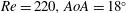 $Re=220,AoA=18^{\circ }$
and wavenumber
$Re=220,AoA=18^{\circ }$
and wavenumber
 $\unicode[STIX]{x1D6FD}=1$
. Shown are the damping rate and frequency of the leading Kelvin–Helmholtz mode at these conditions, obtained using the nektar++ time stepping code. It can be seen that an increase of the domain in the downstream direction in both the
$\unicode[STIX]{x1D6FD}=1$
. Shown are the damping rate and frequency of the leading Kelvin–Helmholtz mode at these conditions, obtained using the nektar++ time stepping code. It can be seen that an increase of the domain in the downstream direction in both the
 $x$
and the
$x$
and the
 $y$
spatial directions produces less stable flow. However, eigenvalue computations using the matrix-forming code FreeFEM++ and a fully unstructured grid, at convergence in any of the domains used by nektar++ code also produces a damped leading eigenvalue with characteristics analogous to those delivered by the time stepping code. Analogous results have been obtained on all three airfoils at different sets of parameters.
$y$
spatial directions produces less stable flow. However, eigenvalue computations using the matrix-forming code FreeFEM++ and a fully unstructured grid, at convergence in any of the domains used by nektar++ code also produces a damped leading eigenvalue with characteristics analogous to those delivered by the time stepping code. Analogous results have been obtained on all three airfoils at different sets of parameters.
Table 7. Effect of domain extent on the modal analysis for the basic flow at
 $Re=220,AoA=18^{\circ }$
and wavenumber
$Re=220,AoA=18^{\circ }$
and wavenumber
 $\unicode[STIX]{x1D6FD}=1$
.
$\unicode[STIX]{x1D6FD}=1$
.

A.2 Non-modal stability analysis
The numerical integrity of the transient growth analysis results has been checked also by repeating selected runs in domains of different extent. The three domains employed for this exercise are
 $D1:[-15,50]\times [-15,15]$
,
$D1:[-15,50]\times [-15,15]$
,
 $D2:[-40,50]\times [-15,15]$
and
$D2:[-40,50]\times [-15,15]$
and
 $D3:[-40,100]\times [-15,15]$
. In chord length units
$D3:[-40,100]\times [-15,15]$
. In chord length units
 $D1$
represents the domain on which most analyses were run with all airfoils,
$D1$
represents the domain on which most analyses were run with all airfoils,
 $D2$
is extended in the upstream spatial direction, in order to assess the degree by which the adjoint eigenvectors are captured and
$D2$
is extended in the upstream spatial direction, in order to assess the degree by which the adjoint eigenvectors are captured and
 $D3$
is the largest domain, which is extended in both the upstream and the downstream spatial directions. New meshes were generated for each of these analyses, base flows were run in the new meshes and the adjoint looping was performed in the same mesh used for the base flow calculation.
$D3$
is the largest domain, which is extended in both the upstream and the downstream spatial directions. New meshes were generated for each of these analyses, base flows were run in the new meshes and the adjoint looping was performed in the same mesh used for the base flow calculation.
The convergence in time of the transient growth results has been tested on the NACA 0015 airfoil at
 $Re=200,AoA=15^{\circ }$
at two distinct wavenumber values,
$Re=200,AoA=15^{\circ }$
at two distinct wavenumber values,
 $\unicode[STIX]{x1D6FD}=0$
and
$\unicode[STIX]{x1D6FD}=0$
and
 $\unicode[STIX]{x03C0}$
, after a short time in the direct-adjoint looping,
$\unicode[STIX]{x03C0}$
, after a short time in the direct-adjoint looping,
 $\unicode[STIX]{x1D70F}=0.1$
, using time steps of
$\unicode[STIX]{x1D70F}=0.1$
, using time steps of
 $\unicode[STIX]{x0394}t=1\times 10^{-3}$
and
$\unicode[STIX]{x0394}t=1\times 10^{-3}$
and
 $2\times 10^{-3}$
and polynomial orders
$2\times 10^{-3}$
and polynomial orders
 $p=5,7$
and 9. Results for
$p=5,7$
and 9. Results for
 $G(\unicode[STIX]{x1D70F})$
obtained after 50 and 100 time steps are identical up to the fifth significant digit.
$G(\unicode[STIX]{x1D70F})$
obtained after 50 and 100 time steps are identical up to the fifth significant digit.
The results of figure 19, obtained on the NACA 0015 at
 $Re=200,AoA=18^{\circ }$
and being typical of those obtained on the other two airfoils, show that the maximum gain associated with the
$Re=200,AoA=18^{\circ }$
and being typical of those obtained on the other two airfoils, show that the maximum gain associated with the
 $\unicode[STIX]{x1D6FD}=0$
wavenumber (two-dimensional flow) is somewhat reduced when the largest domain is used. However, the relative difference of the absolute values of
$\unicode[STIX]{x1D6FD}=0$
wavenumber (two-dimensional flow) is somewhat reduced when the largest domain is used. However, the relative difference of the absolute values of
 $G$
obtained at the same time
$G$
obtained at the same time
 $\unicode[STIX]{x1D70F}$
in the smallest and the largest domains is less than 20 % at its maximum, while the order of magnitude change in
$\unicode[STIX]{x1D70F}$
in the smallest and the largest domains is less than 20 % at its maximum, while the order of magnitude change in
 $G(\unicode[STIX]{x1D70F})$
at all times is well captured by the smallest domain. An analogous result (actually better in terms of maximum relative difference) is seen as regards the maximum singular values,
$G(\unicode[STIX]{x1D70F})$
at all times is well captured by the smallest domain. An analogous result (actually better in terms of maximum relative difference) is seen as regards the maximum singular values,
 $\unicode[STIX]{x1D70E}_{max}$
, obtained in the different domains. Since the cost of the numerical solutions obtained in domain
$\unicode[STIX]{x1D70E}_{max}$
, obtained in the different domains. Since the cost of the numerical solutions obtained in domain
 $D3$
is more than double that in
$D3$
is more than double that in
 $D1$
, the non-modal analyses discussed in the main body of the paper were performed in domain
$D1$
, the non-modal analyses discussed in the main body of the paper were performed in domain
 $D1$
.
$D1$
.

Figure 19. Dependence of
 $G(\unicode[STIX]{x1D70F})$
(a) and the maximum singular value
$G(\unicode[STIX]{x1D70F})$
(a) and the maximum singular value
 $\unicode[STIX]{x1D70E}_{max}$
(b) on the extent of the analysis domain for the 0015 airfoil at
$\unicode[STIX]{x1D70E}_{max}$
(b) on the extent of the analysis domain for the 0015 airfoil at
 $Re=200,AoA=18^{\circ }$
.
$Re=200,AoA=18^{\circ }$
.
A.3 Floquet analysis
Floquet analysis of flow around a NACA 0012 airfoil was performed by Tsiloufas et al. (Reference Tsiloufas, Gioria and Meneghini2009), whose results at
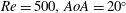 $Re=500,AoA=20^{\circ }$
have been used to validate the present work. First a time-periodic flow at these conditions is computed and subsequently the Floquet multiplier
$Re=500,AoA=20^{\circ }$
have been used to validate the present work. First a time-periodic flow at these conditions is computed and subsequently the Floquet multiplier
 $\unicode[STIX]{x1D707}$
is computed at each value of the spanwise wavenumber parameter
$\unicode[STIX]{x1D707}$
is computed at each value of the spanwise wavenumber parameter
 $\unicode[STIX]{x1D6FD}$
. The modulus of
$\unicode[STIX]{x1D6FD}$
. The modulus of
 $\unicode[STIX]{x1D707}$
determines whether the periodic orbit is stable or unstable. The Semtex code was used for the base flow computation, while its linearized version was employed to perform secondary Floquet instability analysis. The base flow was computed in domains of size
$\unicode[STIX]{x1D707}$
determines whether the periodic orbit is stable or unstable. The Semtex code was used for the base flow computation, while its linearized version was employed to perform secondary Floquet instability analysis. The base flow was computed in domains of size
 $x\in [-15,100]\times y\in [-20,20]$
, the oscillation period at each set of parameters was identified and the base flow results for one period were interpolated in the domain
$x\in [-15,100]\times y\in [-20,20]$
, the oscillation period at each set of parameters was identified and the base flow results for one period were interpolated in the domain
 $x\in [-3,16]\times y\in [-3,3]$
using up to 32 planes in order to ensure convergence of the Floquet multipliers. Gauss–Lobatto–Legendre basis functions have been employed for the spatial discretization of the
$x\in [-3,16]\times y\in [-3,3]$
using up to 32 planes in order to ensure convergence of the Floquet multipliers. Gauss–Lobatto–Legendre basis functions have been employed for the spatial discretization of the
 $Oxy$
macro-elements, while a Fourier expansion is used along the spanwise direction, as discussed in § 3, along with a polynomial order
$Oxy$
macro-elements, while a Fourier expansion is used along the spanwise direction, as discussed in § 3, along with a polynomial order
 $p=7$
on each macro-element described previously, a Krylov dimension
$p=7$
on each macro-element described previously, a Krylov dimension
 $=12$
, an eigenvalue convergence criterion of
$=12$
, an eigenvalue convergence criterion of
 $tol_{Arnoldi}=10^{-6}$
and a maximum number of Arnoldi iterations
$tol_{Arnoldi}=10^{-6}$
and a maximum number of Arnoldi iterations
 $N_{Arnoldi}=40$
. Figure 20 shows comparison of the results of Tsiloufas et al. (Reference Tsiloufas, Gioria and Meneghini2009) and the present computations. Note that the figure is symmetric with respect to a change of sign in
$N_{Arnoldi}=40$
. Figure 20 shows comparison of the results of Tsiloufas et al. (Reference Tsiloufas, Gioria and Meneghini2009) and the present computations. Note that the figure is symmetric with respect to a change of sign in
 $\unicode[STIX]{x1D6FD}$
. The rather good agreement obtained, despite the different codes and meshing strategies used, verifies the present methodology which has subsequently been applied to analyse time-periodic flow instability on the three NACA airfoils using the same parameters as those employed to analyse instability in the wake of the NACA 0012 profile.
$\unicode[STIX]{x1D6FD}$
. The rather good agreement obtained, despite the different codes and meshing strategies used, verifies the present methodology which has subsequently been applied to analyse time-periodic flow instability on the three NACA airfoils using the same parameters as those employed to analyse instability in the wake of the NACA 0012 profile.

Figure 20. Comparison of
 $\unicode[STIX]{x1D707}$
dependence on
$\unicode[STIX]{x1D707}$
dependence on
 $\unicode[STIX]{x1D6FD}$
, as obtained in the present work by Semtex for the NACA 0012 airfoil at
$\unicode[STIX]{x1D6FD}$
, as obtained in the present work by Semtex for the NACA 0012 airfoil at
 $Re=500,AoA=20^{\circ }$
, against literature results (Tsiloufas et al.
Reference Tsiloufas, Gioria and Meneghini2009).
$Re=500,AoA=20^{\circ }$
, against literature results (Tsiloufas et al.
Reference Tsiloufas, Gioria and Meneghini2009).
Additional cross-verifications of the secondary instability analysis results have been performed using the respective modules of the Semtex and nektar++ codes which, although they are based on the same theoretical concepts (Barkley et al.
Reference Barkley, Blackburn and Sherwin2008), follow entirely different implementation paths as regards meshing of the geometries in question. Selected runs have been performed using the NACA 4415 airfoil at
 $Re=500,AoA=20^{\circ }$
, which resulted in differences in the value of the leading Floquet multipliers,
$Re=500,AoA=20^{\circ }$
, which resulted in differences in the value of the leading Floquet multipliers,
 $\unicode[STIX]{x1D707}$
, obtained by the two codes in the fifth significant figure, implying a relative error of
$\unicode[STIX]{x1D707}$
, obtained by the two codes in the fifth significant figure, implying a relative error of
 ${\approx}0.3\,\%$
. Finally, selected direct simulations have been performed at
${\approx}0.3\,\%$
. Finally, selected direct simulations have been performed at
 $\unicode[STIX]{x1D6FD}=0$
in order to verify that the dominant mode has a value of
$\unicode[STIX]{x1D6FD}=0$
in order to verify that the dominant mode has a value of
 $\unicode[STIX]{x1D707}_{1}=1$
, and the value of the second Floquet multiplier is
$\unicode[STIX]{x1D707}_{1}=1$
, and the value of the second Floquet multiplier is
 $\unicode[STIX]{x1D707}_{2}<1$
. In all comparison cases, the origin of the largest differences between the two sets of results was found to be the estimate of the period, as discussed in § 4.4 and presented in table 5.
$\unicode[STIX]{x1D707}_{2}<1$
. In all comparison cases, the origin of the largest differences between the two sets of results was found to be the estimate of the period, as discussed in § 4.4 and presented in table 5.


