


1 Introduction
With the advent of supersonic and transonic aircraft, a particular type of flow separation that results from a strong interaction between shock waves and boundary layers attracted intense attention of researchers. Such shock wave/boundary layer interactions (SBLI) occur on many parts of aircraft such as wings, control surfaces, intakes etc. and can be quite detrimental to the performance of the aircraft. Many theoretical, numerical and experimental investigations have since been conducted to fully understand the phenomenon of SBLI for more than half a century. Especially well-known studies, which have contributed to our theoretical understanding of this problem, are by Lighthill (Reference Lighthill1953), Gadd (Reference Gadd1957), Chapman, Kuehn & Larson (Reference Chapman, Kuehn and Larson1958), Brown & Stewartson (Reference Brown and Stewartson1969), Neiland (Reference Neiland1969), Stewartson & Williams (Reference Stewartson and Williams1969), Messiter (Reference Messiter1970), Neiland (Reference Neiland1970) and Neiland (Reference Neiland1973). The major advance in understanding laminar SBLI and separation was made by Brown & Stewartson (Reference Brown and Stewartson1969), Neiland (Reference Neiland1969), Stewartson & Williams (Reference Stewartson and Williams1969) and Neiland (Reference Neiland1970). They developed a rigorous theory based on an asymptotic approach to the full Navier–Stokes equations in which the interacting boundary layer is divided into three layers (the ‘triple deck’); the viscous sublayer adjacent to the wall, the largely inviscid rotational flow in the main or middle layer and the outer inviscid irrotational (potential) flow. The triple-deck theory enables the effects of pressure perturbations caused by the shock wave on the boundary layer in each of these layers to be taken into account then by appropriately matching the boundary conditions of each layer, it yields a self-consistent set of equations which can be solved either numerically or analytically. The solutions then yield the characteristic parameters of laminar SBLI, such as separation, pressure plateau, peak pressures and the upstream influence. More elaborate interpretations of the subtleties of the separation and reattachment processes and the characteristics of laminar SBLI have been given by Smith (Reference Smith1986), Smith & Khorrami (Reference Smith and Khorrami1991) and Korolev, Gajjar & Ruban (Reference Korolev, Gajjar and Ruban2002). Although the triple-deck theory is an asymptotic theory strictly valid only for very high Reynolds number flows, it has been shown to give reasonable estimates of parameters even for the moderate Reynolds number flows encountered in many experimental situations (Rizzetta, Burggraf & Jenson Reference Rizzetta, Burggraf and Jenson1978; Burggraf et al. Reference Burggraf, Rizzetta, Werle and Vatsa1979; Katzer Reference Katzer1989).
Hypersonic SBLIs have attracted the attention of researchers since the seventies and eighties with the arrival of the age of the space shuttle and other space planes flying at hypersonic speeds. Major contributions to hypersonic SBLI have been due to Neiland (Reference Neiland1973), Brown, Stewartson & Williams (Reference Brown, Stewartson and Williams1975), Rizzetta et al. (Reference Rizzetta, Burggraf and Jenson1978), Gajjar & Smith (Reference Gajjar and Smith1983) and Smith & Khorrami (Reference Smith and Khorrami1991). Thermal effects in hypersonic boundary layers, particularly wall cooling and its effects on SBLI, have also been investigated in recent years and analysed in terms of triple-deck theory (Brown, Cheng & Lee Reference Brown, Cheng and Lee1990; Seddougui, Bowles & Smith Reference Seddougui, Bowles and Smith1991; Kerimbekov, Ruban & Walker Reference Kerimbekov, Ruban and Walker1994; Cassel, Ruban & Walker Reference Cassel, Ruban and Walker1995, Reference Cassel, Ruban and Walker1996; Neiland, Sokolov & Shvedchenko Reference Neiland, Sokolov and Shvedchenko2009; Shvedchenko Reference Shvedchenko2009). Moreover, Khorrami & Smith (Reference Khorrami and Smith1994) presented complete solutions to the hypersonic interactive boundary layer for a semi-infinite plate and thin airfoils, which included both the effects of wall enthalpy and the viscous interaction parameter on the upstream influence. They also looked at the effects of velocity slip and temperature jump. A comprehensive account of hypersonic SBLI and separation and application of triple-deck theory has been given in reviews by Stewartson (Reference Stewartson1974), Smith (Reference Smith1986), Sychev et al. (Reference Sychev, Ruban, Sychev and Korolev1998) and Neiland et al. (Reference Neiland, Boglepov, Dudin and Lipatov2008). An analytical solution for reattachment flow has been obtained in Smith (Reference Smith1988).
Herein, we present an investigation pertaining to hypersonic viscous interaction and separation using the so-called leading edge separation configuration. This particular configuration was first considered and investigated by Chapman et al. (Reference Chapman, Kuehn and Larson1958) at supersonic Mach numbers and moderate to high Reynolds numbers. The hypersonic SBLI on such a configuration does not appear to have been investigated in detail so far and was the motivation for the present study. Wall temperature effects on this type of separation are also considered.
2 Model geometry and flow conditions
In order to understand the basic characteristics of hypersonic flow separation, we consider a leading edge separation configuration. Chapman et al. (Reference Chapman, Kuehn and Larson1958), as mentioned earlier, first used this configuration as it is particularly well suited for theoretical analysis, and the authors used it as such to develop their isentropic recompression theory to predict base pressures behind bluff bodies. Their rationale in using this geometry was that it precludes the effects of a pre-existing boundary layer and hence made it easy to use laminar mixing layer theory. Chapman et al. (Reference Chapman, Kuehn and Larson1958) point out further that, in fact, the leading edge separation arrangement can be considered as a limiting case of both separation behind a base and compression corner, wherein the distance from the leading edge to separation point
 $\unicode[STIX]{x0394}s$
reduces to zero (figure 1). Later, Stewartson (Reference Stewartson1964) and Brown & Stewartson (Reference Brown and Stewartson1969) mentioned leading edge separation without taking it further except to say that it is worth exploring the assumptions, made by Chapman et al. (Reference Chapman, Kuehn and Larson1958) from a more rigorous standpoint. The investigation of Chapman et al. (Reference Chapman, Kuehn and Larson1958) was restricted to low to moderate supersonic Mach numbers and moderate to high Reynolds numbers. It is, therefore, of sufficient interest to examine the properties of such a separation under viscous flow conditions, when the Mach numbers are high and Reynolds numbers are low, as encountered during hypersonic flight at high altitude such as re-entry. The present investigation is restricted to two-dimensional steady hypersonic laminar separated flows.
$\unicode[STIX]{x0394}s$
reduces to zero (figure 1). Later, Stewartson (Reference Stewartson1964) and Brown & Stewartson (Reference Brown and Stewartson1969) mentioned leading edge separation without taking it further except to say that it is worth exploring the assumptions, made by Chapman et al. (Reference Chapman, Kuehn and Larson1958) from a more rigorous standpoint. The investigation of Chapman et al. (Reference Chapman, Kuehn and Larson1958) was restricted to low to moderate supersonic Mach numbers and moderate to high Reynolds numbers. It is, therefore, of sufficient interest to examine the properties of such a separation under viscous flow conditions, when the Mach numbers are high and Reynolds numbers are low, as encountered during hypersonic flight at high altitude such as re-entry. The present investigation is restricted to two-dimensional steady hypersonic laminar separated flows.

Figure 1. Evolution of separation in compression corners: (a) finite separation length; (b) leading edge separation (
 $\unicode[STIX]{x0394}s\rightarrow 0$
).
$\unicode[STIX]{x0394}s\rightarrow 0$
).
 $\unicode[STIX]{x0394}s$
is the distance from the leading edge to separation.
$\unicode[STIX]{x0394}s$
is the distance from the leading edge to separation.

Figure 2. Schematic of flow structure of hypersonic leading edge separation (baseline case) and geometry.
Figure 2 shows a schematic of the leading edge configuration used in the numerical study with main flow features. Here, the corner angle at
 $B$
is selected so that it is large enough to ensure separation at (or very near) the sharp leading edge at
$B$
is selected so that it is large enough to ensure separation at (or very near) the sharp leading edge at
 $A$
. This configuration is equivalent to a compression corner of deflection angle
$A$
. This configuration is equivalent to a compression corner of deflection angle
 $55^{\circ }$
, whose upstream plate
$55^{\circ }$
, whose upstream plate
 $AB$
has been tilted around the corner at a large positive incidence angle of
$AB$
has been tilted around the corner at a large positive incidence angle of
 $30^{\circ }$
, instead of being parallel to the free stream (see Chapman et al.
Reference Chapman, Kuehn and Larson1958). Ideally, after expansion, a thin shear layer, in which the velocity varies from zero to the local external stream value, emanates from
$30^{\circ }$
, instead of being parallel to the free stream (see Chapman et al.
Reference Chapman, Kuehn and Larson1958). Ideally, after expansion, a thin shear layer, in which the velocity varies from zero to the local external stream value, emanates from
 $A$
and reattaches at
$A$
and reattaches at
 $C$
. A large recirculation region is thus formed and bounded by
$C$
. A large recirculation region is thus formed and bounded by
 $ABC$
in which a shear layer
$ABC$
in which a shear layer
 $AC$
separates it from the outer inviscid flow. Under hypersonic conditions, due to strong viscous effects at the leading edge, the expansion is preceded by a weak leading edge shock wave.
$AC$
separates it from the outer inviscid flow. Under hypersonic conditions, due to strong viscous effects at the leading edge, the expansion is preceded by a weak leading edge shock wave.
Table 1 shows the flow conditions used in numerical simulations. These flow conditions were previously obtained from a free-piston-driven shock tunnel as per Park, Gai & Neely (Reference Park, Gai and Neely2010). In table 1,
 $h,T,p$
and
$h,T,p$
and
 $Re$
, denote the specific enthalpy, temperature, pressure, density and Reynolds number, respectively, whereas subscripts ‘
$Re$
, denote the specific enthalpy, temperature, pressure, density and Reynolds number, respectively, whereas subscripts ‘
 $o$
’ and
$o$
’ and
 $\infty$
refer to the reservoir and free-stream conditions, respectively. To investigate the effects of wall temperature
$\infty$
refer to the reservoir and free-stream conditions, respectively. To investigate the effects of wall temperature
 $T_{w}$
, three isothermal walls of 165, 300 and 800 K, and an adiabatic wall have been considered. The selection of wall temperatures essentially represent the free-stream temperature, a baseline, an intermediate and a limiting case of an adiabatic wall. These wall temperatures correspond, respectively, to wall to stagnation temperature ratios
$T_{w}$
, three isothermal walls of 165, 300 and 800 K, and an adiabatic wall have been considered. The selection of wall temperatures essentially represent the free-stream temperature, a baseline, an intermediate and a limiting case of an adiabatic wall. These wall temperatures correspond, respectively, to wall to stagnation temperature ratios
 $s_{w}$
of 0.05, 0.1, 0.25 and 0.88, and reflect a range varying from strong cooling to no heat flux into the wall.
$s_{w}$
of 0.05, 0.1, 0.25 and 0.88, and reflect a range varying from strong cooling to no heat flux into the wall.
Table 1. Nozzle reservoir and free-stream conditions (Park et al. Reference Park, Gai and Neely2010).
3 Theoretical considerations
3.1 The triple-deck structure of a compressible boundary layer
Figure 3 shows a basic triple-deck structure centred at a compression corner with a typical separation velocity profile as shown by the red dashed line. Here, the
 $x$
and
$x$
and
 $y$
coordinates express the streamwise and transverse directions, respectively, and
$y$
coordinates express the streamwise and transverse directions, respectively, and
 $\unicode[STIX]{x1D716}=Re^{-1/8}$
is the controlling parameter in the triple-deck theory, where
$\unicode[STIX]{x1D716}=Re^{-1/8}$
is the controlling parameter in the triple-deck theory, where
 $Re$
is a characteristic Reynolds number, assumed asymptotically large, based on the free stream and length
$Re$
is a characteristic Reynolds number, assumed asymptotically large, based on the free stream and length
 $L_{e}$
. The boundary layer profile in the interaction region is characterised in terms of a main, upper and lower deck, and each is assigned a thickness in terms
$L_{e}$
. The boundary layer profile in the interaction region is characterised in terms of a main, upper and lower deck, and each is assigned a thickness in terms
 $\unicode[STIX]{x1D716}$
. The main deck in which the fluid is largely inviscid and rotational is of the order
$\unicode[STIX]{x1D716}$
. The main deck in which the fluid is largely inviscid and rotational is of the order
 $\unicode[STIX]{x1D716}^{4}$
. The upper deck, where the fluid is inviscid and irrotational, is of the order
$\unicode[STIX]{x1D716}^{4}$
. The upper deck, where the fluid is inviscid and irrotational, is of the order
 $\unicode[STIX]{x1D716}^{3}$
. Finally, the lower deck, where viscous effects are dominant, is of the order
$\unicode[STIX]{x1D716}^{3}$
. Finally, the lower deck, where viscous effects are dominant, is of the order
 $\unicode[STIX]{x1D716}^{5}$
. The pressure (
$\unicode[STIX]{x1D716}^{5}$
. The pressure (
 $\unicode[STIX]{x0394}p$
) and velocity (
$\unicode[STIX]{x0394}p$
) and velocity (
 $\unicode[STIX]{x0394}u$
) perturbations are assumed to be of the order
$\unicode[STIX]{x0394}u$
) perturbations are assumed to be of the order
 $\unicode[STIX]{x1D716}^{2}$
and
$\unicode[STIX]{x1D716}^{2}$
and
 $\unicode[STIX]{x1D716}$
, respectively. The pressure and velocity perturbations are assumed to spread over a streamwise distance (
$\unicode[STIX]{x1D716}$
, respectively. The pressure and velocity perturbations are assumed to spread over a streamwise distance (
 $\unicode[STIX]{x0394}x$
) of the scale
$\unicode[STIX]{x0394}x$
) of the scale
 $\unicode[STIX]{x1D716}^{3}$
called the interaction region. The scaled value of the corner angle
$\unicode[STIX]{x1D716}^{3}$
called the interaction region. The scaled value of the corner angle
 $\unicode[STIX]{x1D6FC}$
is of the order
$\unicode[STIX]{x1D6FC}$
is of the order
 $\unicode[STIX]{x1D716}^{2}$
, and the normalised distance from the leading edge to the corner is 1.
$\unicode[STIX]{x1D716}^{2}$
, and the normalised distance from the leading edge to the corner is 1.

Figure 3. Triple-deck structure in corner flows. Dashed line is a separated velocity profile.
Analyses of laminar SBLI, based on triple-deck theory were given by Neiland (Reference Neiland1969), Stewartson & Williams (Reference Stewartson and Williams1969) and Neiland (Reference Neiland1970). The basis of this theory is that the whole interaction process is controlled by the lower deck, the equations of which are essentially those of the incompressible boundary layer. Neiland (Reference Neiland1970), Neiland (Reference Neiland1973), Stewartson (Reference Stewartson1975), Rizzetta et al. (Reference Rizzetta, Burggraf and Jenson1978), Gajjar & Smith (Reference Gajjar and Smith1983), Smith & Khorrami (Reference Smith and Khorrami1991) and Sychev et al. (Reference Sychev, Ruban, Sychev and Korolev1998) have since shown that the triple-deck approach, by using appropriate boundary conditions, is equally valid in hypersonic interactive boundary layers with (or without) wall cooling. In terms of scaled variables (Stewartson & Williams Reference Stewartson and Williams1969; Rizzetta et al. Reference Rizzetta, Burggraf and Jenson1978; Gajjar & Smith Reference Gajjar and Smith1983), the governing equations for a steady two-dimensional flow are,
 $$\begin{eqnarray}\displaystyle & \displaystyle \frac{\unicode[STIX]{x2202}U}{\unicode[STIX]{x2202}X}+\frac{\unicode[STIX]{x2202}V}{Y}=0, & \displaystyle\end{eqnarray}$$
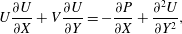 $$\begin{eqnarray}\displaystyle & \displaystyle U\frac{\unicode[STIX]{x2202}U}{\unicode[STIX]{x2202}X}+V\frac{\unicode[STIX]{x2202}U}{\unicode[STIX]{x2202}Y}=-\frac{\unicode[STIX]{x2202}P}{\unicode[STIX]{x2202}X}+\frac{\unicode[STIX]{x2202}^{2}U}{\unicode[STIX]{x2202}Y^{2}}, & \displaystyle\end{eqnarray}$$
 $$\begin{eqnarray}\displaystyle & \displaystyle \frac{\unicode[STIX]{x2202}P}{\unicode[STIX]{x2202}Y}=0, & \displaystyle\end{eqnarray}$$
where
 $U$
and
$U$
and
 $V$
are the streamwise and transverse velocities, respectively,
$V$
are the streamwise and transverse velocities, respectively,
 $X$
is the streamwise direction,
$X$
is the streamwise direction,
 $Y$
is the transverse direction and
$Y$
is the transverse direction and
 $P$
is the pressure. The governing boundary condition are as
$P$
is the pressure. The governing boundary condition are as
 $Y\rightarrow \infty$
,
$Y\rightarrow \infty$
,
 $U\rightarrow Y+A(X)$
, at the wall,
$U\rightarrow Y+A(X)$
, at the wall,
 $U=V=0$
, and as
$U=V=0$
, and as
 $X\rightarrow \infty$
,
$X\rightarrow \infty$
,
 $(U,V,P^{^{\prime }}A)\rightarrow (Y,0,0,0)$
, where the prime notation indicates the derivative in the streamwise direction. Here,
$(U,V,P^{^{\prime }}A)\rightarrow (Y,0,0,0)$
, where the prime notation indicates the derivative in the streamwise direction. Here,
 $A(X)$
is an arbitrary function describing the change in displacement thickness in a self-induced separation.
$A(X)$
is an arbitrary function describing the change in displacement thickness in a self-induced separation.
For a supersonic outer flow, the pressure perturbation in
 $P$
is obtained by invoking the Ackeret relation so that
$P$
is obtained by invoking the Ackeret relation so that
 $P(X)=-A^{^{\prime }}(X)$
. For hypersonic flow, the pressure–displacement relation is obtained through the tangent-wedge approximation as was first proposed by Neiland (Reference Neiland1970) and discussed in Stewartson (Reference Stewartson1975), Gajjar & Smith (Reference Gajjar and Smith1983) and Smith & Khorrami (Reference Smith and Khorrami1991). A more generalised expression, which includes the effects of wall cooling is given by Brown et al. (Reference Brown, Cheng and Lee1990) in the form,
$P(X)=-A^{^{\prime }}(X)$
. For hypersonic flow, the pressure–displacement relation is obtained through the tangent-wedge approximation as was first proposed by Neiland (Reference Neiland1970) and discussed in Stewartson (Reference Stewartson1975), Gajjar & Smith (Reference Gajjar and Smith1983) and Smith & Khorrami (Reference Smith and Khorrami1991). A more generalised expression, which includes the effects of wall cooling is given by Brown et al. (Reference Brown, Cheng and Lee1990) in the form,
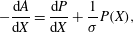 $$\begin{eqnarray}-\frac{\text{d}A}{\text{d}X}=\frac{\text{d}P}{\text{d}X}+\frac{1}{\unicode[STIX]{x1D70E}}P(X),\end{eqnarray}$$
where
 $\unicode[STIX]{x1D70E}$
is a parameter, which includes the effects of both hypersonic viscous interaction parameter
$\unicode[STIX]{x1D70E}$
is a parameter, which includes the effects of both hypersonic viscous interaction parameter
 $\bar{\unicode[STIX]{x1D712}}$
and wall cooling.
$\bar{\unicode[STIX]{x1D712}}$
and wall cooling.
 $\unicode[STIX]{x1D70E}$
is given in Brown et al. (Reference Brown, Cheng and Lee1990) as,
$\unicode[STIX]{x1D70E}$
is given in Brown et al. (Reference Brown, Cheng and Lee1990) as,
 $$\begin{eqnarray}\unicode[STIX]{x1D70E}=\left(\frac{s_{w}^{\ast }}{s_{w}}\right)^{4\unicode[STIX]{x1D714}+2},\end{eqnarray}$$
where
 $s_{w}$
is the wall temperature to stagnation temperature ratio
$s_{w}$
is the wall temperature to stagnation temperature ratio
 $T_{w}/T_{o}$
, and
$T_{w}/T_{o}$
, and
 $s_{w}^{\ast }$
is the critical wall temperature ratio defined in Cheng (Reference Cheng1993) as,
$s_{w}^{\ast }$
is the critical wall temperature ratio defined in Cheng (Reference Cheng1993) as,
 $$\begin{eqnarray}s_{w}^{\ast }\sim \frac{T^{\ast }}{T_{o}}\sim \left[\unicode[STIX]{x1D706}^{5}\unicode[STIX]{x1D6FE}^{-1/2}\left(\frac{2}{\unicode[STIX]{x1D6FE}-1}\right)^{2}\bar{\unicode[STIX]{x1D712}}\right]^{1/(4\unicode[STIX]{x1D714}+2)},\end{eqnarray}$$
where
 $\unicode[STIX]{x1D706}$
is a normalised undisturbed wall shear,
$\unicode[STIX]{x1D706}$
is a normalised undisturbed wall shear,
 $\unicode[STIX]{x1D6FE}$
is the specific heat ratio of air and
$\unicode[STIX]{x1D6FE}$
is the specific heat ratio of air and
 $\bar{\unicode[STIX]{x1D712}}$
is the hypersonic viscous interaction parameter evaluated at the corner.
$\bar{\unicode[STIX]{x1D712}}$
is the hypersonic viscous interaction parameter evaluated at the corner.
 $\unicode[STIX]{x1D714}$
is the viscosity index, which ranges from 0.5 to 1 and for strong wall cooling, the lower limit is usually taken (see Brown et al.
Reference Brown, Cheng and Lee1990). The term
$\unicode[STIX]{x1D714}$
is the viscosity index, which ranges from 0.5 to 1 and for strong wall cooling, the lower limit is usually taken (see Brown et al.
Reference Brown, Cheng and Lee1990). The term
 $2/(\unicode[STIX]{x1D6FE}-1)$
is called the Newtonian factor, and when
$2/(\unicode[STIX]{x1D6FE}-1)$
is called the Newtonian factor, and when
 $(\unicode[STIX]{x1D6FE}-1)/2\ll 1$
and
$(\unicode[STIX]{x1D6FE}-1)/2\ll 1$
and
 $M\gg 1$
, the use of tangent-wedge approximation of Neiland (Reference Neiland1970) is justified. If the boundary layer upstream of the interaction is a fully developed Blasius profile, then with
$M\gg 1$
, the use of tangent-wedge approximation of Neiland (Reference Neiland1970) is justified. If the boundary layer upstream of the interaction is a fully developed Blasius profile, then with
 $\unicode[STIX]{x1D6FE}$
= 1.4 and
$\unicode[STIX]{x1D6FE}$
= 1.4 and
 $\unicode[STIX]{x1D706}$
= 0.332, we get,
$\unicode[STIX]{x1D706}$
= 0.332, we get,
 $$\begin{eqnarray}\unicode[STIX]{x1D70E}\sim 0.085\bar{\unicode[STIX]{x1D712}}s_{w}^{-4},\end{eqnarray}$$
which shows that
 $\unicode[STIX]{x1D70E}$
is proportional to the hypersonic viscous interaction parameter, but more importantly, rapidly increases with decreasing wall temperature.
$\unicode[STIX]{x1D70E}$
is proportional to the hypersonic viscous interaction parameter, but more importantly, rapidly increases with decreasing wall temperature.
The hypersonic viscous interaction parameter usually defined as
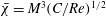 $\bar{\unicode[STIX]{x1D712}}=M^{3}(C/Re)^{1/2}$
(Hayes & Probstein Reference Hayes and Probstein1959) is based on the distance from the leading edge
$\bar{\unicode[STIX]{x1D712}}=M^{3}(C/Re)^{1/2}$
(Hayes & Probstein Reference Hayes and Probstein1959) is based on the distance from the leading edge
 $A$
to the corner
$A$
to the corner
 $B$
. Various authors, for example, Rizzetta et al. (Reference Rizzetta, Burggraf and Jenson1978), Smith & Khorrami (Reference Smith and Khorrami1991), Korolev et al. (Reference Korolev, Gajjar and Ruban2002), Neiland et al. (Reference Neiland, Sokolov and Shvedchenko2009) and Shvedchenko (Reference Shvedchenko2009) have used the distance from the leading edge to the compression corner as the characteristic dimension of the problem. Brown et al. (Reference Brown, Cheng and Lee1990), on the other hand, have taken the distance from the plate leading edge to the beginning of interaction as the characteristic length, while Katzer (Reference Katzer1989) used the distance from the leading edge to the point of shockwave impingement on a plate as the characteristic dimension. Herein, to be consistent, we use the distance from the leading edge to the corner (length
$B$
. Various authors, for example, Rizzetta et al. (Reference Rizzetta, Burggraf and Jenson1978), Smith & Khorrami (Reference Smith and Khorrami1991), Korolev et al. (Reference Korolev, Gajjar and Ruban2002), Neiland et al. (Reference Neiland, Sokolov and Shvedchenko2009) and Shvedchenko (Reference Shvedchenko2009) have used the distance from the leading edge to the compression corner as the characteristic dimension of the problem. Brown et al. (Reference Brown, Cheng and Lee1990), on the other hand, have taken the distance from the plate leading edge to the beginning of interaction as the characteristic length, while Katzer (Reference Katzer1989) used the distance from the leading edge to the point of shockwave impingement on a plate as the characteristic dimension. Herein, to be consistent, we use the distance from the leading edge to the corner (length
 $AB$
in figure 2) as the characteristic dimension for the evaluation of
$AB$
in figure 2) as the characteristic dimension for the evaluation of
 $\bar{\unicode[STIX]{x1D712}}$
. In the expression for
$\bar{\unicode[STIX]{x1D712}}$
. In the expression for
 $\bar{\unicode[STIX]{x1D712}}$
,
$\bar{\unicode[STIX]{x1D712}}$
,
 $C$
is the Chapman–Rubesin constant.
$C$
is the Chapman–Rubesin constant.
It has been shown by Gajjar & Smith (Reference Gajjar and Smith1983) that in the special case of
 $\unicode[STIX]{x1D70E}\rightarrow \infty$
, the expression
$\unicode[STIX]{x1D70E}\rightarrow \infty$
, the expression
 $P(X)=-A(X)$
reduces to simple hypersonic free interaction that exhibits power-law growth of pressure with
$P(X)=-A(X)$
reduces to simple hypersonic free interaction that exhibits power-law growth of pressure with
 $X$
. Brown et al. (Reference Brown, Cheng and Lee1990) point out that for large (but finite) value of
$X$
. Brown et al. (Reference Brown, Cheng and Lee1990) point out that for large (but finite) value of
 $\unicode[STIX]{x1D70E}$
, a plateau in
$\unicode[STIX]{x1D70E}$
, a plateau in
 $P$
(for large
$P$
(for large
 $X$
) is possible. Their numerical calculations, however, did not indicate a plateau for
$X$
) is possible. Their numerical calculations, however, did not indicate a plateau for
 $\unicode[STIX]{x1D70E}>10$
. Gajjar & Smith (Reference Gajjar and Smith1983) also showed that
$\unicode[STIX]{x1D70E}>10$
. Gajjar & Smith (Reference Gajjar and Smith1983) also showed that
 $P(X)=-A(X)$
can equally describe a supercritical hydraulic jump in a shallow liquid layer down an inclined plane.
$P(X)=-A(X)$
can equally describe a supercritical hydraulic jump in a shallow liquid layer down an inclined plane.
A somewhat different approach was taken by Neiland (Reference Neiland1973) and his associates (see for example, Kerimbekov et al. Reference Kerimbekov, Ruban and Walker1994, Cassel et al. Reference Cassel, Ruban and Walker1995 and Cassel et al. Reference Cassel, Ruban and Walker1996). Kerimbekov et al. (Reference Kerimbekov, Ruban and Walker1994) describes the interactive equation as,
 $$\begin{eqnarray}-\frac{\text{d}A}{\text{d}X}=P(X)-N^{3/4}\frac{\text{d}P}{\text{d}X},\end{eqnarray}$$
where
 $N$
is the Nieland number (Cassel et al.
Reference Cassel, Ruban and Walker1996), defined as,
$N$
is the Nieland number (Cassel et al.
Reference Cassel, Ruban and Walker1996), defined as,
 $$\begin{eqnarray}N=S|{\mathcal{L}}|^{4/3}.\end{eqnarray}$$
When
 $N\ll 1$
, the flow is subcritical (wall cooling), supercritical (wall heating) when
$N\ll 1$
, the flow is subcritical (wall cooling), supercritical (wall heating) when
 $N\gg 1$
, and transcritical (approaching adiabatic) when
$N\gg 1$
, and transcritical (approaching adiabatic) when
 $N\sim O(1)$
. This is equivalent to
$N\sim O(1)$
. This is equivalent to
 $s_{w}^{\ast }/s_{w}\ll 1$
,
$s_{w}^{\ast }/s_{w}\ll 1$
,
 $s_{w}^{\ast }/s_{w}\gg 1$
and
$s_{w}^{\ast }/s_{w}\gg 1$
and
 $s_{w}^{\ast }/sw\sim O(1)$
, respectively, in Brown et al. (Reference Brown, Cheng and Lee1990) terminology.
$s_{w}^{\ast }/sw\sim O(1)$
, respectively, in Brown et al. (Reference Brown, Cheng and Lee1990) terminology.
Numerical calculations on a compression corner in hypersonic flow carried out by Cassel et al. (Reference Cassel, Ruban and Walker1996), based on Neiland’s approach, show that a pressure plateau exists, for all values of
 $N$
, after separation and downstream of the corner, in contrast to Brown et al. (Reference Brown, Cheng and Lee1990). They, also, found that increasing
$N$
, after separation and downstream of the corner, in contrast to Brown et al. (Reference Brown, Cheng and Lee1990). They, also, found that increasing
 $N$
(equivalently
$N$
(equivalently
 $\unicode[STIX]{x1D70E}$
) causes the separation point to move towards the corner. The separation region extent
$\unicode[STIX]{x1D70E}$
) causes the separation point to move towards the corner. The separation region extent
 $\unicode[STIX]{x0394}x$
, as shown by Neiland et al. (Reference Neiland, Sokolov and Shvedchenko2009), also decreases with decreasing
$\unicode[STIX]{x0394}x$
, as shown by Neiland et al. (Reference Neiland, Sokolov and Shvedchenko2009), also decreases with decreasing
 $s_{w}$
(increasing
$s_{w}$
(increasing
 $N$
), since,
$N$
), since,
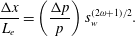 $$\begin{eqnarray}\frac{\unicode[STIX]{x0394}x}{L_{e}}=\left(\frac{\unicode[STIX]{x0394}p}{p}\right)s_{w}^{(2\unicode[STIX]{x1D714}+1)/2}.\end{eqnarray}$$
These hypersonic triple-deck theories are based on certain important assumptions. Firstly, they are asymptotic theories valid at high Reynolds numbers, and generally assume
 $\bar{\unicode[STIX]{x1D712}}\sim O(1)$
or less. The Newtonian approximation that
$\bar{\unicode[STIX]{x1D712}}\sim O(1)$
or less. The Newtonian approximation that
 $(\unicode[STIX]{x1D6FE}-1)/2\ll 1$
, and
$(\unicode[STIX]{x1D6FE}-1)/2\ll 1$
, and
 $M\gg 1$
is, in general, required to hold. It is assumed, therein, that prior to the interaction with a sudden pressure disturbance (typically, a compression corner or an incident shock wave), the boundary layer is fully developed, and the separation process resulting from the interaction is ‘free’ and spontaneous (Chapman et al.
Reference Chapman, Kuehn and Larson1958; Neiland Reference Neiland1969; Stewartson & Williams Reference Stewartson and Williams1969). Such interaction is not influenced by downstream conditions and is independent of the agency provoking separation. Finally, it is assumed that the interaction region is small (
$M\gg 1$
is, in general, required to hold. It is assumed, therein, that prior to the interaction with a sudden pressure disturbance (typically, a compression corner or an incident shock wave), the boundary layer is fully developed, and the separation process resulting from the interaction is ‘free’ and spontaneous (Chapman et al.
Reference Chapman, Kuehn and Larson1958; Neiland Reference Neiland1969; Stewartson & Williams Reference Stewartson and Williams1969). Such interaction is not influenced by downstream conditions and is independent of the agency provoking separation. Finally, it is assumed that the interaction region is small (
 ${\sim}Re^{-3/8}$
), and separation is small enough to be contained within it. In recent years, however, there have been attempts to study large-scale separations within the general framework of hypersonic triple-deck theory by Neiland (Reference Neiland1973), Brown et al. (Reference Brown, Stewartson and Williams1975), Brown et al. (Reference Brown, Cheng and Lee1990), Smith & Khorrami (Reference Smith and Khorrami1991), Sychev et al. (Reference Sychev, Ruban, Sychev and Korolev1998), Neiland et al. (Reference Neiland, Sokolov and Shvedchenko2009) and Shvedchenko (Reference Shvedchenko2009), with some success.
${\sim}Re^{-3/8}$
), and separation is small enough to be contained within it. In recent years, however, there have been attempts to study large-scale separations within the general framework of hypersonic triple-deck theory by Neiland (Reference Neiland1973), Brown et al. (Reference Brown, Stewartson and Williams1975), Brown et al. (Reference Brown, Cheng and Lee1990), Smith & Khorrami (Reference Smith and Khorrami1991), Sychev et al. (Reference Sychev, Ruban, Sychev and Korolev1998), Neiland et al. (Reference Neiland, Sokolov and Shvedchenko2009) and Shvedchenko (Reference Shvedchenko2009), with some success.
In what follows, the leading edge separation problem will be investigated and analysed in the context of hypersonic triple-deck framework and large separated regions.
4 Computational approach
4.1 General description of numerical solver and assumptions
The numerical simulations were carried out using the compressible Navier–Stokes solver, US3D. The code was developed by Candler and his associates at the University of Minnesota (Nompelis & Candler Reference Nompelis and Candler2014; Candler et al. Reference Candler, Johnson, Nompelis, Gidzak, Subbareddy and Barnhardt2015), and is capable of modelling both perfect and real gases. The code has been validated for simple and complex geometries (Drayna, Nompelis & Candler Reference Drayna, Nompelis and Candler2006; Holden et al. Reference Holden, Wadhams, MacLean and Dufrene2013; Candler, Subbareddy & Brock Reference Candler, Subbareddy and Brock2014) at hypersonic speeds. In the real gas simulations, the code solves the conservation equations by using law of mass action for chemical species, whereas reaction rates are given in the Arrhenius form. Equilibrium constants are determined by using the NASA Lewis CEA database. The code uses the two-temperature kinetic model of Park (Reference Park1993), but in this instance, a combined translational–rotational and vibrational temperature is used for the perfect gas. The energy exchange is based on the Landau–Teller equation, and vibrational relaxation times are based on Millikan & White (Reference Millikan and White1963) empirical correlations.
The code uses a finite volume method to solve three-dimensional Navier–Stokes equations, and is capable of both steady-state and transient solutions. The steady-state solution is obtained by using the modified Steger–Warming flux vector splitting method (Candler et al. Reference Candler, Johnson, Nompelis, Gidzak, Subbareddy and Barnhardt2015), and monotone-upstream-conservative-limited scheme (Van Leer Reference Van Leer1979) to obtain higher-order spatial accuracy. To maintain low dissipation, as it is necessary in hypersonic simulations, the code uses the Osher limiter by default (Nompelis & Candler Reference Nompelis and Candler2014). To achieve faster convergence, the code uses the data-parallel-line-relaxation approach (Wright, Candler & Bose Reference Wright, Candler and Bose1998), and in the present study, the implicit scheme is used.
The simulations assumed perfect gas air with constant specific heat ratio
 $\unicode[STIX]{x1D6FE}$
of 1.4, and transport properties were evaluated using Wilke’s mixing rule (Wilke Reference Wilke1950; Blottner, Johnson & Ellis Reference Blottner, Johnson and Ellis1971). For the flow conditions given in table 1, air is assumed to be a continuum, laminar and without slip or temperature jump at the wall. Further, the wall is assumed to be non-catalytic.
$\unicode[STIX]{x1D6FE}$
of 1.4, and transport properties were evaluated using Wilke’s mixing rule (Wilke Reference Wilke1950; Blottner, Johnson & Ellis Reference Blottner, Johnson and Ellis1971). For the flow conditions given in table 1, air is assumed to be a continuum, laminar and without slip or temperature jump at the wall. Further, the wall is assumed to be non-catalytic.
4.2 Grid generation and boundary conditions
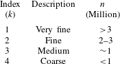
In the present study, structured grids were generated for all wall temperatures to carry out a grid independence study. Table 2 describes these grids based on their number of cells
 $n$
and overall quality. Here, ‘coarse’ is used to describe grids with
$n$
and overall quality. Here, ‘coarse’ is used to describe grids with
 $n<1$
million, ‘medium’, for grids with
$n<1$
million, ‘medium’, for grids with
 $n\sim 1$
million, ‘fine’, for grids with
$n\sim 1$
million, ‘fine’, for grids with
 $n$
between 2 and 3 million and finally, ‘very fine’, for grids with
$n$
between 2 and 3 million and finally, ‘very fine’, for grids with
 $n$
much greater than 3 million.
$n$
much greater than 3 million.
Table 2. Description of grids used in the simulations where
 $n$
is the number of cells.
$n$
is the number of cells.
In figure 4, the coarse grid of the baseline case (
 $s_{w}=0.1$
) is shown. The blue line defines the computational domain boundaries. In the solver, the boundary conditions were the same for all the grids used, except for minor differences in the specification of wall temperature. The domain boundaries are labelled in figure 4 and correspond to the appropriate boundary condition. Edges 1 and 2 are the supersonic velocity inlets, edges 3 and 6 are the outflow, edges 4–6 are the walls specified either as isothermal walls as in
$s_{w}=0.1$
) is shown. The blue line defines the computational domain boundaries. In the solver, the boundary conditions were the same for all the grids used, except for minor differences in the specification of wall temperature. The domain boundaries are labelled in figure 4 and correspond to the appropriate boundary condition. Edges 1 and 2 are the supersonic velocity inlets, edges 3 and 6 are the outflow, edges 4–6 are the walls specified either as isothermal walls as in
 $s_{w}=0.05$
, 0.1 and 0.25, or adiabatic as in
$s_{w}=0.05$
, 0.1 and 0.25, or adiabatic as in
 $s_{w}=0.88$
. Given the critical flow features near the leading edge, corner and reattachment, cells in these regions were clustered as necessary. To ensure a good flow resolution near the walls, a constant first cell height
$s_{w}=0.88$
. Given the critical flow features near the leading edge, corner and reattachment, cells in these regions were clustered as necessary. To ensure a good flow resolution near the walls, a constant first cell height
 $\unicode[STIX]{x0394}s_{w}$
of
$\unicode[STIX]{x0394}s_{w}$
of
 $1~\unicode[STIX]{x03BC}\text{m}$
was used for all grids. A Courant–Friedrichs–Lewy number larger than 200 was possible for most simulations. Starting from the coarse grid, grid refinement was achieved by successively increasing the number of cells
$1~\unicode[STIX]{x03BC}\text{m}$
was used for all grids. A Courant–Friedrichs–Lewy number larger than 200 was possible for most simulations. Starting from the coarse grid, grid refinement was achieved by successively increasing the number of cells
 $n$
by a factor of
$n$
by a factor of
 ${\sim}2.1$
on average.
${\sim}2.1$
on average.

Figure 4. Baseline grid. The blue line defines the computational domain boundaries. Numbers seen on the edges refer to the boundary conditions. Edge 5 is 20 mm for all grids. To accommodate the increase in separation length due to wall temperature, edge 4 was extended to 80 mm and 100 mm for
 $s_{w}=0.25$
and
$s_{w}=0.25$
and
 $s_{w}=0.88$
, respectively.
$s_{w}=0.88$
, respectively.
4.3 Convergence studies
To verify the accuracy of the numerical solver, grid solutions were checked for both iterative and overall grid convergence. Iterative convergence is typically done by monitoring residuals as reported by the solver, and the solution is said to be iteratively converged if the residuals drop by at least 5 orders of magnitude. Overall grid convergence is determined by using an appropriate grid error analysis method. Additional convergence checks were made by checking changes in surface parameters as they settle to their steady-state values with successive iterations. In the present case, the parameters of interest are the shear stress
 $\unicode[STIX]{x1D70F}_{w}^{\ast }$
, pressure
$\unicode[STIX]{x1D70F}_{w}^{\ast }$
, pressure
 $p_{w}^{\ast }$
and heat flux
$p_{w}^{\ast }$
and heat flux
 $q_{w}^{\ast }$
. Superscript ‘*’ refers to normalised quantities of the dimensional shear stress and surface pressure by the dynamic pressure
$q_{w}^{\ast }$
. Superscript ‘*’ refers to normalised quantities of the dimensional shear stress and surface pressure by the dynamic pressure
 $0.5\unicode[STIX]{x1D70C}U_{\infty }^{2}$
, dimensional heat flux by
$0.5\unicode[STIX]{x1D70C}U_{\infty }^{2}$
, dimensional heat flux by
 $0.5\unicode[STIX]{x1D70C}U_{\infty }^{3}$
and
$0.5\unicode[STIX]{x1D70C}U_{\infty }^{3}$
and
 $s^{\ast }$
is the distance along the wall normalised by the expansion length
$s^{\ast }$
is the distance along the wall normalised by the expansion length
 $AB$
. In figure 5(a,c,e), these quantities are shown only for
$AB$
. In figure 5(a,c,e), these quantities are shown only for
 $s_{w}=0.1$
, 0.25 and 0.88. For
$s_{w}=0.1$
, 0.25 and 0.88. For
 $s_{w}=0.05$
, convergence was justifiably deduced from the baseline grid (
$s_{w}=0.05$
, convergence was justifiably deduced from the baseline grid (
 $s_{w}=0.1$
) by showing similar separation characteristics. Based on these figures, we first note that there are no visible changes in surface parameters, starting from the medium grids towards finer grids. These grids also showed consistent flow features and an overall increase in the size of separation with grid refinement. Details near the corner (figure 5
b,f), and near the leading edge (figure 5
d), also show similar flow features in terms of the boundary layer length and resolution of corner eddies. Based on these observations, grids with
$s_{w}=0.1$
) by showing similar separation characteristics. Based on these figures, we first note that there are no visible changes in surface parameters, starting from the medium grids towards finer grids. These grids also showed consistent flow features and an overall increase in the size of separation with grid refinement. Details near the corner (figure 5
b,f), and near the leading edge (figure 5
d), also show similar flow features in terms of the boundary layer length and resolution of corner eddies. Based on these observations, grids with
 $n$
more than 1 million cells can be said to have achieved convergence. Interpretations of these flow features will be presented in the results and discussion section.
$n$
more than 1 million cells can be said to have achieved convergence. Interpretations of these flow features will be presented in the results and discussion section.

Figure 5. Convergence data for (a) global shear stress
 $\unicode[STIX]{x1D70F}_{w}^{\ast }$
; (b) shear stress near the corner; (c) global surface pressure
$\unicode[STIX]{x1D70F}_{w}^{\ast }$
; (b) shear stress near the corner; (c) global surface pressure
 $p_{w}^{\ast }$
; (d) pressure near the leading edge; (e) global heat flux
$p_{w}^{\ast }$
; (d) pressure near the leading edge; (e) global heat flux
 $q_{w}^{\ast }$
; (f) heat flux near the corner. Black line:
$q_{w}^{\ast }$
; (f) heat flux near the corner. Black line:
 $s_{w}=0.1$
; red line:
$s_{w}=0.1$
; red line:
 $s_{w}=0.25$
; blue line:
$s_{w}=0.25$
; blue line:
 $s_{w}=0.88$
. Long-dashed line: grid 1; solid line: grid 2; dashed line: grid 3; dotted line: grid 4. (see table 2).
$s_{w}=0.88$
. Long-dashed line: grid 1; solid line: grid 2; dashed line: grid 3; dotted line: grid 4. (see table 2).
4.4 Grid error analysis
In the present study, the mixed-order method was used to carry out the grid error analysis. The method is considered appropriate for flows with discontinuities such as shock waves (Roy Reference Roy2003). Starting with the series solution of the discretisation error,
 $$\begin{eqnarray}f=f_{exact}+g_{1}h+g_{2}h^{2}+O(h^{3}).\end{eqnarray}$$
Here,
 $f$
denotes the grid solution,
$f$
denotes the grid solution,
 $h$
is the cell size,
$h$
is the cell size,
 $f_{exact}$
is the solution as
$f_{exact}$
is the solution as
 $h\rightarrow 0$
, the values of
$h\rightarrow 0$
, the values of
 $g$
are the order coefficients, and subscripts ‘1’ and ‘2’ are the orders of the error. Equation (4.1) requires that the solution to be within the asymptotic range and to contain no discontinuities. The mixed-order method, then, can be achieved by keeping the first- and second-order terms in (4.1), and expanding (4.1) for at least three grids. For an arbitrary mesh,
$g$
are the order coefficients, and subscripts ‘1’ and ‘2’ are the orders of the error. Equation (4.1) requires that the solution to be within the asymptotic range and to contain no discontinuities. The mixed-order method, then, can be achieved by keeping the first- and second-order terms in (4.1), and expanding (4.1) for at least three grids. For an arbitrary mesh,
 $f_{exact}$
can be obtained by using,
$f_{exact}$
can be obtained by using,
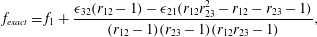 $$\begin{eqnarray}f_{exact}=f_{1}+\frac{\unicode[STIX]{x1D716}_{32}(r_{12}-1)-\unicode[STIX]{x1D716}_{21}(r_{12}r_{23}^{2}-r_{12}-r_{23}-1)}{(r_{12}-1)(r_{23}-1)(r_{12}r_{23}-1)},\end{eqnarray}$$
where,
 $\unicode[STIX]{x1D716}_{32}=f_{3}-f_{2}$
,
$\unicode[STIX]{x1D716}_{32}=f_{3}-f_{2}$
,
 $\unicode[STIX]{x1D716}_{21}=f_{2}-f_{1}$
,
$\unicode[STIX]{x1D716}_{21}=f_{2}-f_{1}$
,
 $r_{12}=h_{1}/h_{2}$
,
$r_{12}=h_{1}/h_{2}$
,
 $r_{23}=h_{2}/h_{3}$
.
$r_{23}=h_{2}/h_{3}$
.
It is critical to point out that (4.2) is still an approximation, which is accurate to third order.
 $f_{exact}$
is calculated at separation and reattachment to obtain the spatial error,
$f_{exact}$
is calculated at separation and reattachment to obtain the spatial error,
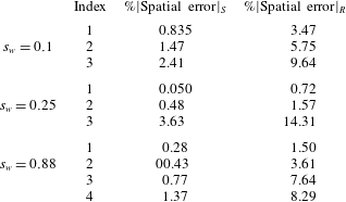
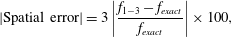 $$\begin{eqnarray}|\text{Spatial error}|=3\left|\frac{f_{1-3}-f_{exact}}{f_{exact}}\right|\times 100,\end{eqnarray}$$
noting that at separation, the expansion length
 $L_{e}$
is more appropriate in the denominator of (4.3) to avoid any division near zero (Roy Reference Roy2003). The factor ‘3’ is a safety factor to obtain conservative estimate of the error. Table 3 shows the error values in per cent at separation (subscript ‘
$L_{e}$
is more appropriate in the denominator of (4.3) to avoid any division near zero (Roy Reference Roy2003). The factor ‘3’ is a safety factor to obtain conservative estimate of the error. Table 3 shows the error values in per cent at separation (subscript ‘
 $S$
’) and reattachment (subscript ‘
$S$
’) and reattachment (subscript ‘
 $R$
’), and also at different wall temperatures. A systematic drop in the error with grid refinement can be seen and indicate grid convergence. The spatial errors also seem to be maintained within
$R$
’), and also at different wall temperatures. A systematic drop in the error with grid refinement can be seen and indicate grid convergence. The spatial errors also seem to be maintained within
 $4\,\%$
and
$4\,\%$
and
 $15\,\%$
at separation and reattachment, respectively, for all grids. The results presented in § 4 are based on the fine grid solutions (Index 2).
$15\,\%$
at separation and reattachment, respectively, for all grids. The results presented in § 4 are based on the fine grid solutions (Index 2).
Table 3. Spatial errors evaluated at separation and reattachment (see (4.3)).
5 Results and discussion
5.1 Basic features of wall temperatures effects on laminar hypersonic leading edge separation
Figures 6–8 show the shear stress, pressure and heat flux distributions, where the superscript ‘
 $\ast$
’ again denotes the values normalised by
$\ast$
’ again denotes the values normalised by
 $0.5\unicode[STIX]{x1D70C}_{\infty }U^{2}$
for the shear stress and pressure, and
$0.5\unicode[STIX]{x1D70C}_{\infty }U^{2}$
for the shear stress and pressure, and
 $0.5\unicode[STIX]{x1D70C}_{\infty }U^{3}$
for the heat flux against the normalised distance
$0.5\unicode[STIX]{x1D70C}_{\infty }U^{3}$
for the heat flux against the normalised distance
 $s^{\ast }=s/L_{e}$
, where
$s^{\ast }=s/L_{e}$
, where
 $s$
is the wetted distance and
$s$
is the wetted distance and
 $L_{e}$
is the length of the expansion surface. The results are shown for the four temperature ratios under consideration (
$L_{e}$
is the length of the expansion surface. The results are shown for the four temperature ratios under consideration (
 $s_{w}$
of 0.05, 0.1, 0.25 and 0.88).
$s_{w}$
of 0.05, 0.1, 0.25 and 0.88).
Considering the shear stress first, near the leading edge (figure 6
a), separation (indicated by filled circles) is evidenced by the shear stress crossing the zero line (or changing sign), which occurs within a distance of less than
 $10\,\%$
from the leading edge, for all wall temperatures. We also note that separation is pushed upstream towards the leading edge as
$10\,\%$
from the leading edge, for all wall temperatures. We also note that separation is pushed upstream towards the leading edge as
 $s_{w}$
is increased. The steep fall in shear stress prior to separation is due to the leading edge singularity. The open circles in figure 6(a) show locations of beginning of interaction,
$s_{w}$
is increased. The steep fall in shear stress prior to separation is due to the leading edge singularity. The open circles in figure 6(a) show locations of beginning of interaction,
 $s_{1}^{\ast }$
. In the shear stress curve, the pressure rise appears to coincide with a ‘knee’ for
$s_{1}^{\ast }$
. In the shear stress curve, the pressure rise appears to coincide with a ‘knee’ for
 $s_{w}=0.05$
–0.25 that becomes less obvious for the adiabatic wall, and the distance from the leading edge to
$s_{w}=0.05$
–0.25 that becomes less obvious for the adiabatic wall, and the distance from the leading edge to
 $s_{1}^{\ast }$
becomes less with increased wall temperature.
$s_{1}^{\ast }$
becomes less with increased wall temperature.

Figure 6. Wall temperature effect on shear stress: (a) close up near the leading edge and (b) global shear stress. Dashed green line:
 $s_{w}=0.05$
; solid black line:
$s_{w}=0.05$
; solid black line:
 $s_{w}=0.1$
; dotted red line:
$s_{w}=0.1$
; dotted red line:
 $s_{w}=0.25$
; long-dashed blue line:
$s_{w}=0.25$
; long-dashed blue line:
 $s_{w}=0.88$
. Closed circles: separation; open circles: beginning of interaction; squares: reattachment.
$s_{w}=0.88$
. Closed circles: separation; open circles: beginning of interaction; squares: reattachment.
In figure 6(b), within the separated region, we see two minima in the shear stress distribution. The first minimum occurs soon after separation (closed circles), and the second is immediately followed by reattachment (open squares). The minimum before reattachment is found to be greater in magnitude than that after separation. The occurrence of two minima is typical of SBLI with large separated regions. Rizzetta et al. (Reference Rizzetta, Burggraf and Jenson1978), Bodonyi & Smith (Reference Bodonyi and Smith1986), Elliott & Smith (Reference Elliott and Smith1986), Smith (Reference Smith1988), Katzer (Reference Katzer1989) and Smith & Khorrami (Reference Smith and Khorrami1991) have investigated this feature of SBLI in detail and attributed the second minimum to a reverse flow singularity/breakdown. Subsequently, Korolev et al. (Reference Korolev, Gajjar and Ruban2002) and Neiland et al. (Reference Neiland, Sokolov and Shvedchenko2009) have shown that there need not be such a restriction (of a singularity) prior to reattachment in large-scale separations in terms of some critical scaled angle
 $\unicode[STIX]{x1D703}Re^{-1/4}$
, where
$\unicode[STIX]{x1D703}Re^{-1/4}$
, where
 $\unicode[STIX]{x1D703}$
typically represents an incident shock or some other compressive disturbance such as a compression corner. Our results further showed that the flow transitions smoothly from separation to reattachment without any breakdown, and the second minimum becomes progressively shallower and more negative with increasing wall temperature (figure 6
b).
$\unicode[STIX]{x1D703}$
typically represents an incident shock or some other compressive disturbance such as a compression corner. Our results further showed that the flow transitions smoothly from separation to reattachment without any breakdown, and the second minimum becomes progressively shallower and more negative with increasing wall temperature (figure 6
b).
Continuing with figure 6(b), after reattachment (indicated by open squares), we note that the shear stress reaches a maximum, and depending on the wall temperature, shows double peaks. This double peak is most prominent for the temperature ratios of 0.05 and 0.1. The first peak appears only slightly higher than the second at
 $s_{w}=0.05$
, whereas with
$s_{w}=0.05$
, whereas with
 $s_{w}=0.1$
, the second peak higher than the first. With moderate cooling at
$s_{w}=0.1$
, the second peak higher than the first. With moderate cooling at
 $s_{w}=0.25$
, the difference between the first and second peaks appear to be the greatest. Finally, in the adiabatic case (
$s_{w}=0.25$
, the difference between the first and second peaks appear to be the greatest. Finally, in the adiabatic case (
 $s_{w}$
= 0.88), the first peak is absent and only a single sharp peak is seen with a lower magnitude than the other wall temperatures. The first peak, when examined, coincides with the minimum neck area during recompression and the second peak with the triple point of separation and recompression shocks.
$s_{w}$
= 0.88), the first peak is absent and only a single sharp peak is seen with a lower magnitude than the other wall temperatures. The first peak, when examined, coincides with the minimum neck area during recompression and the second peak with the triple point of separation and recompression shocks.
The presence of these peaks immediately following reattachment is due, firstly, to the formation of a neck (because of the sonic line being very close to the surface in the reattached boundary layer at high Mach numbers) preceding the intersection of separation and recompression shock system forming a triple point, also close to the surface springing an expansion fan leading to high shear stress. The double peak seems to be a feature of high Mach number hypersonic SBLI and this feature is confirmed at these flow conditions in the computations done by R. Hillier (Private communication, 2015) using a different numerical code.
Figure 7 shows the corresponding surface pressure near the leading edge (a) and global surface pressure (b). Near the leading edge, the pressures, on reaching a minimum soon after the leading edge, show a sudden rise towards separation in which its slope rises with rising wall temperature. Further, the boundary layer extent prior to separation can be determined from the distance from the leading edge to the beginning of interaction. In the case of the coldest wall considered,
 $s_{w}=0.05$
, the boundary layer reaches
$s_{w}=0.05$
, the boundary layer reaches
 $8\,\%$
of the distance from the leading edge and reduces to nearly
$8\,\%$
of the distance from the leading edge and reduces to nearly
 $4\,\%$
for the adiabatic wall. These results are consistent with the findings of Khorrami & Smith (Reference Khorrami and Smith1994), who showed that the upstream influence distance for hypersonic flow over a semi-infinite flat plate is reduced by both a higher wall temperature and lower viscous interaction parameter (defined as
$4\,\%$
for the adiabatic wall. These results are consistent with the findings of Khorrami & Smith (Reference Khorrami and Smith1994), who showed that the upstream influence distance for hypersonic flow over a semi-infinite flat plate is reduced by both a higher wall temperature and lower viscous interaction parameter (defined as
 $M/Re^{1/6}$
). They looked at various wall temperatures and cases where the viscous interaction parameter, as per their definition, is equal to or greater than 2. The viscous interaction parameter calculated for the present wall temperatures varies between 2.6 for
$M/Re^{1/6}$
). They looked at various wall temperatures and cases where the viscous interaction parameter, as per their definition, is equal to or greater than 2. The viscous interaction parameter calculated for the present wall temperatures varies between 2.6 for
 $s_{w}$
0.05, and 3 for the
$s_{w}$
0.05, and 3 for the
 $s_{w}$
0.88. Here, the effect of increasing wall temperature, in reducing the upstream influence distance, appears to outweigh the effect of viscous interaction parameter. The greater drop in pressure with wall temperature is also in accordance with Khorrami and Smith’s (Reference Khorrami and Smith1994) findings. Neiland et al. (Reference Neiland, Sokolov and Shvedchenko2009) and Shvedchenko (Reference Shvedchenko2009) have further noted that the leading edge has no critical effect on the solution downstream and disturbances dissipate quite rapidly with distance downstream. After separation, the pressures reach a plateau that spans over the whole expansion surface. With the increase in wall temperature, we see that the magnitude of the plateau and length of the separated region are increased. Compared to the length of the separated region (the straight distance between
$s_{w}$
0.88. Here, the effect of increasing wall temperature, in reducing the upstream influence distance, appears to outweigh the effect of viscous interaction parameter. The greater drop in pressure with wall temperature is also in accordance with Khorrami and Smith’s (Reference Khorrami and Smith1994) findings. Neiland et al. (Reference Neiland, Sokolov and Shvedchenko2009) and Shvedchenko (Reference Shvedchenko2009) have further noted that the leading edge has no critical effect on the solution downstream and disturbances dissipate quite rapidly with distance downstream. After separation, the pressures reach a plateau that spans over the whole expansion surface. With the increase in wall temperature, we see that the magnitude of the plateau and length of the separated region are increased. Compared to the length of the separated region (the straight distance between
 $S$
and
$S$
and
 $R$
) of the adiabatic wall, the separation length at the lower wall temperatures,
$R$
) of the adiabatic wall, the separation length at the lower wall temperatures,
 $s_{w}=0.25$
, 0.1 and 0.05 is reduced by
$s_{w}=0.25$
, 0.1 and 0.05 is reduced by
 $32\,\%$
,
$32\,\%$
,
 $39.5\,\%$
and
$39.5\,\%$
and
 $43.5\,\%$
, respectively. These features are consistent with those found by Neiland et al. (Reference Neiland, Sokolov and Shvedchenko2009).
$43.5\,\%$
, respectively. These features are consistent with those found by Neiland et al. (Reference Neiland, Sokolov and Shvedchenko2009).

Figure 7. Wall temperature effect on surface pressure: (a) close-up near the leading edge and (b) global surface pressure. Dashed green line:
 $s_{w}=0.05$
; solid black line:
$s_{w}=0.05$
; solid black line:
 $s_{w}=0.1$
; dotted red line:
$s_{w}=0.1$
; dotted red line:
 $s_{w}=0.25$
; long-dashed blue line:
$s_{w}=0.25$
; long-dashed blue line:
 $s_{w}=0.88$
. Closed circles: separation; open circles: beginning of interaction; squares: reattachment.
$s_{w}=0.88$
. Closed circles: separation; open circles: beginning of interaction; squares: reattachment.
Examination of pressure distributions in figure 7(b) further reveals additional features. For instance, prior to reattachment, the pressure shows a perceptible decrease from the plateau value before rising again. This ‘dip’ in the plateau pressure is indicative of a secondary separation near the corner. This has been noted and commented upon previously by Smith & Khorrami (Reference Smith and Khorrami1991) and more recently by Korolev et al. (Reference Korolev, Gajjar and Ruban2002). Shvedchenko (Reference Shvedchenko2009) has also noted that while this dip in pressure is sharp and rapid at high Reynolds numbers, there is a ‘smearing’ effect at lower Reynolds numbers. In the present instance, the Reynolds numbers are of the order of
 $1\times 10^{3}$
so that these features are spread out and diffused. Another aspect is that in post-reattachment the pressures show similar double peaks as in the shear stress distribution, in which the first is associated with the neck region and second with the triple point of the separation and reattachment shocks along with an emanating expansion wave and a slip line. The intersection of separation and reattachment shocks accompanied by an expansion and a slip line is usually referred to as Edney type VI shock/shock interference (Edney Reference Edney1968).
$1\times 10^{3}$
so that these features are spread out and diffused. Another aspect is that in post-reattachment the pressures show similar double peaks as in the shear stress distribution, in which the first is associated with the neck region and second with the triple point of the separation and reattachment shocks along with an emanating expansion wave and a slip line. The intersection of separation and reattachment shocks accompanied by an expansion and a slip line is usually referred to as Edney type VI shock/shock interference (Edney Reference Edney1968).
Effects of wall temperature on overall heat flux in (b) and in the vicinity of the leading edge (a) are shown in figure 8. We observe that with decreasing wall temperature, the heat flux increases as expected and is zero for the adiabatic case. The maximum heat flux is seen in figure 8(b) as a single sharp peak with no obvious second peak, as in shear stress and pressure, although at
 $s_{w}=0.25$
, there is a hint of a ‘knee’ shortly after the peak. The decrease in peak heat flux with increase in wall temperature seems to be a strongly nonlinear function of wall temperature. With increase in
$s_{w}=0.25$
, there is a hint of a ‘knee’ shortly after the peak. The decrease in peak heat flux with increase in wall temperature seems to be a strongly nonlinear function of wall temperature. With increase in
 $s_{w}$
from 0.05 to 0.1, it decreases by 7.5 % but at
$s_{w}$
from 0.05 to 0.1, it decreases by 7.5 % but at
 $s_{w}$
at 0.25, it has decreased by approximately 40 %. A ‘knee’ also appears for
$s_{w}$
at 0.25, it has decreased by approximately 40 %. A ‘knee’ also appears for
 $s_{w}$
0.05 and 0.1 at separation (closed circles in figure 8
a). The beginning of interaction is less distinguishable for the heat flux and is thus not shown.
$s_{w}$
0.05 and 0.1 at separation (closed circles in figure 8
a). The beginning of interaction is less distinguishable for the heat flux and is thus not shown.

Figure 8. Wall temperature effect on heat flux: (a) close-up near the leading edge and (b) global heat flux. Dashed green line:
 $s_{w}=0.05$
; solid black line:
$s_{w}=0.05$
; solid black line:
 $s_{w}=0.1$
; dotted red line:
$s_{w}=0.1$
; dotted red line:
 $s_{w}=0.25$
; long-dashed blue line:
$s_{w}=0.25$
; long-dashed blue line:
 $s_{w}=0.88$
. Closed circles: separation; open circles: beginning of interaction; squares: reattachment.
$s_{w}=0.88$
. Closed circles: separation; open circles: beginning of interaction; squares: reattachment.
Lastly, figure 9 shows the effect of wall temperature, expressed in terms of
 $s_{w}$
, on the locations of separation and reattachment (figure 9
a), separation, reattachment and plateau pressures (figure 9
b) and peak heat flux,
$s_{w}$
, on the locations of separation and reattachment (figure 9
a), separation, reattachment and plateau pressures (figure 9
b) and peak heat flux,
 $q_{w,max}^{\ast }$
(figure 9
c). It is important to note that in order to show these figures on the same scale, we have lowered the order of the reattachment values (location and pressure) by a factor of 10 whilst the others remain unchanged. This exercise is interesting because, due to a dominant nonlinear behaviour, two distinct regions of wall temperature are apparent. First, for
$q_{w,max}^{\ast }$
(figure 9
c). It is important to note that in order to show these figures on the same scale, we have lowered the order of the reattachment values (location and pressure) by a factor of 10 whilst the others remain unchanged. This exercise is interesting because, due to a dominant nonlinear behaviour, two distinct regions of wall temperature are apparent. First, for
 $s_{w}<0.25$
, the effect of wall cooling is greater on separation, and to a lesser degree on the reattachment pressure. And second, for
$s_{w}<0.25$
, the effect of wall cooling is greater on separation, and to a lesser degree on the reattachment pressure. And second, for
 $s_{w}>0.25$
, these features drop towards the adiabatic value, while the reattachment pressure increases towards the adiabatic value. These features seem to indicate the wall temperature effects are greater on reattachment, plateau pressure and maximum heat flux than on separation.
$s_{w}>0.25$
, these features drop towards the adiabatic value, while the reattachment pressure increases towards the adiabatic value. These features seem to indicate the wall temperature effects are greater on reattachment, plateau pressure and maximum heat flux than on separation.

Figure 9. Effects of
 $s_{w}$
on (a) onset of separation (green circles) and reattachment (black diamonds), (b) pressure at separation (red squares); pressure plateau (black diamonds); reattachment (green circles) and (c) peak heat flux,
$s_{w}$
on (a) onset of separation (green circles) and reattachment (black diamonds), (b) pressure at separation (red squares); pressure plateau (black diamonds); reattachment (green circles) and (c) peak heat flux,
 $q_{w,max}^{\ast }$
.
$q_{w,max}^{\ast }$
.
5.2 Flow near the corner
Figure 10(a) shows the shear stress distribution in the vicinity of the corner between
 $0.4\leqslant s^{\ast }\leqslant 2.1$
. The corresponding heat flux and pressure are shown in figure 10(b,c). We note that the shear stress crosses zero, becoming positive, then goes to zero at the vertex after reaching a peak. This is true for all wall temperature studied here. The shear stress then becomes positive again only to reach another peak before becoming negative. This double loop within the main separation bubble is due to the discontinuity at the vertex, where the shear stress must go to zero. The double loop is a manifestation of a secondary corner eddy. The shape and size of this eddy seems to be dependent on the wall temperature.
$0.4\leqslant s^{\ast }\leqslant 2.1$
. The corresponding heat flux and pressure are shown in figure 10(b,c). We note that the shear stress crosses zero, becoming positive, then goes to zero at the vertex after reaching a peak. This is true for all wall temperature studied here. The shear stress then becomes positive again only to reach another peak before becoming negative. This double loop within the main separation bubble is due to the discontinuity at the vertex, where the shear stress must go to zero. The double loop is a manifestation of a secondary corner eddy. The shape and size of this eddy seems to be dependent on the wall temperature.
At
 $s_{w}=0.05$
, the corner eddy is small (and slightly asymmetric) with respect to the vertex. A feature to note here is the emergence of a small third eddy in the region
$s_{w}=0.05$
, the corner eddy is small (and slightly asymmetric) with respect to the vertex. A feature to note here is the emergence of a small third eddy in the region
 $0.4\leqslant s^{\ast }\leqslant 0.6$
. At
$0.4\leqslant s^{\ast }\leqslant 0.6$
. At
 $s_{w}=0.1$
there is a single corner eddy, which has grown to a length nearly half that of the expansion surface, and crosses the corner towards the compression surface. The small third eddy seen at
$s_{w}=0.1$
there is a single corner eddy, which has grown to a length nearly half that of the expansion surface, and crosses the corner towards the compression surface. The small third eddy seen at
 $s_{w}=0.05$
, however, seems to have been swallowed by the larger corner eddy. This is due to the interaction between diffusion and convection of vorticity resulting in stretching of filaments of vorticity at the corner, and the smaller eddy (Burggraf Reference Burggraf1966). The main vortex has moved downstream with its centre towards the compression surface. At
$s_{w}=0.05$
, however, seems to have been swallowed by the larger corner eddy. This is due to the interaction between diffusion and convection of vorticity resulting in stretching of filaments of vorticity at the corner, and the smaller eddy (Burggraf Reference Burggraf1966). The main vortex has moved downstream with its centre towards the compression surface. At
 $s_{w}=0.25$
, we again notice other significant changes: first, the corner eddy has grown much bigger with its centre now almost symmetrically disposed with respect to the vertex, and the main vortex meanwhile has shifted downstream being stretched further. With the adiabatic wall (
$s_{w}=0.25$
, we again notice other significant changes: first, the corner eddy has grown much bigger with its centre now almost symmetrically disposed with respect to the vertex, and the main vortex meanwhile has shifted downstream being stretched further. With the adiabatic wall (
 $s_{w}=0.88$
), both the main vortex and the corner eddy are both stretched and located predominantly on the compression side.
$s_{w}=0.88$
), both the main vortex and the corner eddy are both stretched and located predominantly on the compression side.

Figure 10. Flow near the corner: (a) shear stress, (b) heat flux and (c) pressure. Dashed green line:
 $s_{w}=0.05$
; solid black line:
$s_{w}=0.05$
; solid black line:
 $s_{w}=0.1$
; dotted red line:
$s_{w}=0.1$
; dotted red line:
 $s_{w}=0.25$
; long-dashed blue line:
$s_{w}=0.25$
; long-dashed blue line:
 $s_{w}=0.88$
.
$s_{w}=0.88$
.
It seems clear that both the size and shape of the corner and the main vortex are strongly dependent on the wall temperature and there seems to be a shift downstream with increase in wall temperature. As pointed out by Burggraf (Reference Burggraf1966), the dependence of vorticity and its distribution in the recirculating region seems clearly related to the thermal energy distribution.
Presence of multiple eddies embedded within the main vortex, in a large separated flow, has been noted previously in numerical studies by Neiland et al. (Reference Neiland, Sokolov and Shvedchenko2009) and Shvedchenko (Reference Shvedchenko2009) on ramp-induced separations at large angles (
 $10^{\circ }$
–
$10^{\circ }$
–
 $20^{\circ }$
). Shvedchenko (Reference Shvedchenko2009) identifies a scaled ramp angle as the critical parameter for the occurrence of these multiple vortices independent of the wall temperature. This scaled ramp angle
$20^{\circ }$
). Shvedchenko (Reference Shvedchenko2009) identifies a scaled ramp angle as the critical parameter for the occurrence of these multiple vortices independent of the wall temperature. This scaled ramp angle
 $\unicode[STIX]{x1D709}_{o}$
is defined as
$\unicode[STIX]{x1D709}_{o}$
is defined as
 $\unicode[STIX]{x1D703}Re^{1/4}$
, where
$\unicode[STIX]{x1D703}Re^{1/4}$
, where
 $\unicode[STIX]{x1D703}$
is the geometric angle. Neiland et al. (Reference Neiland, Sokolov and Shvedchenko2009) and Shvedchenko (Reference Shvedchenko2009) show that separation size and occurrence of multiple vortices is a strong function of both
$\unicode[STIX]{x1D703}$
is the geometric angle. Neiland et al. (Reference Neiland, Sokolov and Shvedchenko2009) and Shvedchenko (Reference Shvedchenko2009) show that separation size and occurrence of multiple vortices is a strong function of both
 $\unicode[STIX]{x1D709}_{o}$
and
$\unicode[STIX]{x1D709}_{o}$
and
 $s_{w}$
, and that with increase of both, the separation is pushed upstream towards the leading edge of the plate and the reattachment downstream on the ramp. For angles
$s_{w}$
, and that with increase of both, the separation is pushed upstream towards the leading edge of the plate and the reattachment downstream on the ramp. For angles
 $\unicode[STIX]{x1D703}\geqslant 20^{\circ }$
, separation occurs at the leading edge. Shvedchenko (Reference Shvedchenko2009) delineates various separation stages based on the value of
$\unicode[STIX]{x1D703}\geqslant 20^{\circ }$
, separation occurs at the leading edge. Shvedchenko (Reference Shvedchenko2009) delineates various separation stages based on the value of
 $\unicode[STIX]{x1D709}_{o}$
with the wall temperature having a small or no effect. For example, for small steady separation at the ramp corner,
$\unicode[STIX]{x1D709}_{o}$
with the wall temperature having a small or no effect. For example, for small steady separation at the ramp corner,
 $2\leqslant \unicode[STIX]{x1D709}_{o}\leqslant 3$
for cooled and adiabatic walls alike. For steady secondary separation,
$2\leqslant \unicode[STIX]{x1D709}_{o}\leqslant 3$
for cooled and adiabatic walls alike. For steady secondary separation,
 $5\leqslant \unicode[STIX]{x1D709}_{o}\leqslant 6$
with no effect of the wall temperature. When
$5\leqslant \unicode[STIX]{x1D709}_{o}\leqslant 6$
with no effect of the wall temperature. When
 $\unicode[STIX]{x1D709}_{o}\leqslant 7$
, Shvedchenko (Reference Shvedchenko2009) shows that instability arises in secondary separation giving way to multiple small-scale eddies, and the secondary separation becomes completely unsteady for
$\unicode[STIX]{x1D709}_{o}\leqslant 7$
, Shvedchenko (Reference Shvedchenko2009) shows that instability arises in secondary separation giving way to multiple small-scale eddies, and the secondary separation becomes completely unsteady for
 $\unicode[STIX]{x1D709}_{o}\geqslant 10$
. It should be pointed out here that
$\unicode[STIX]{x1D709}_{o}\geqslant 10$
. It should be pointed out here that
 $\unicode[STIX]{x1D709}_{o}$
as defined by Shvedchenko (Reference Shvedchenko2009) is slightly different from that of Rizzetta (Reference Rizzetta1976), who define the scaled corner angle
$\unicode[STIX]{x1D709}_{o}$
as defined by Shvedchenko (Reference Shvedchenko2009) is slightly different from that of Rizzetta (Reference Rizzetta1976), who define the scaled corner angle
 $\unicode[STIX]{x1D6FC}$
in terms of the triple-deck scales,
$\unicode[STIX]{x1D6FC}$
in terms of the triple-deck scales,
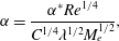 $$\begin{eqnarray}\unicode[STIX]{x1D6FC}=\frac{\unicode[STIX]{x1D6FC}^{\ast }Re^{1/4}}{C^{1/4}\unicode[STIX]{x1D706}^{1/2}M_{e}^{1/2}},\end{eqnarray}$$
which includes the effects of viscosity
 $C$
, wall shear
$C$
, wall shear
 $\unicode[STIX]{x1D706}$
and the Mach number
$\unicode[STIX]{x1D706}$
and the Mach number
 $M_{e}$
at the edge of the boundary layer taking into account all components of the interaction.
$M_{e}$
at the edge of the boundary layer taking into account all components of the interaction.
 $\unicode[STIX]{x1D6FC}^{\ast }$
is the geometric angle in their notation.
$\unicode[STIX]{x1D6FC}^{\ast }$
is the geometric angle in their notation.
A similar expression has been used by Korolev et al. (Reference Korolev, Gajjar and Ruban2002) to identify primary and secondary vortices. They define it as a controlling similarity parameter for the ramp-induced SBLI. According to this criterion, secondary separation occurs when
 $\unicode[STIX]{x1D6FC}\approx 5$
. Our data, based on
$\unicode[STIX]{x1D6FC}\approx 5$
. Our data, based on
 $C$
and
$C$
and
 $\unicode[STIX]{x1D706}$
evaluated for the various wall temperatures, show that the secondary eddy appears in the range of
$\unicode[STIX]{x1D706}$
evaluated for the various wall temperatures, show that the secondary eddy appears in the range of
 $\unicode[STIX]{x1D6FC}$
3–6, the higher value signifying the lowest wall temperature and the lower value the adiabatic wall temperature thereby showing a somewhat higher effect of the wall temperature.
$\unicode[STIX]{x1D6FC}$
3–6, the higher value signifying the lowest wall temperature and the lower value the adiabatic wall temperature thereby showing a somewhat higher effect of the wall temperature.
The heat flux distribution near the corner is shown in figure 10(b). As expected,
 $q_{w}^{\ast }$
goes to zero at the corner vertex and decreases with
$q_{w}^{\ast }$
goes to zero at the corner vertex and decreases with
 $s_{w}$
until it reaches zero for the adiabatic wall. The heat flux distribution for
$s_{w}$
until it reaches zero for the adiabatic wall. The heat flux distribution for
 $s_{w}=0.05$
shows the maximum variation, and the presence of the corner eddy has the effect of reducing
$s_{w}=0.05$
shows the maximum variation, and the presence of the corner eddy has the effect of reducing
 $q_{w}^{\ast }$
for the isothermal walls. The latter is evidenced by the sudden drop near
$q_{w}^{\ast }$
for the isothermal walls. The latter is evidenced by the sudden drop near
 $s^{\ast }=0.4$
for
$s^{\ast }=0.4$
for
 $s_{w}=0.1$
and
$s_{w}=0.1$
and
 $s_{w}=0.25$
, and soon after the nascent eddy (
$s_{w}=0.25$
, and soon after the nascent eddy (
 $s_{w}^{\ast }=0.75$
) at
$s_{w}^{\ast }=0.75$
) at
 $s_{w}=0.05$
. The heat flux also appears to be a mirror image of the shear stress (excluding the adiabatic wall), in the sense that an increase in shear stress is associated with a decrease in the heat flux, and the maxima in shear stress are seen as minima in the heat flux (and vice versa). Figure 10(c), similarly, shows the pressure distribution in the corner region. Though the pressure appears largely constant for all values of
$s_{w}=0.05$
. The heat flux also appears to be a mirror image of the shear stress (excluding the adiabatic wall), in the sense that an increase in shear stress is associated with a decrease in the heat flux, and the maxima in shear stress are seen as minima in the heat flux (and vice versa). Figure 10(c), similarly, shows the pressure distribution in the corner region. Though the pressure appears largely constant for all values of
 $s_{w}$
, we observe a slight drop near the corner. This drop is reduced with the increase in
$s_{w}$
, we observe a slight drop near the corner. This drop is reduced with the increase in
 $s_{w}$
, and reaches a maximum (6.5 %) for
$s_{w}$
, and reaches a maximum (6.5 %) for
 $s_{w}=0.05$
. Downstream, we notice an inflection point coinciding with the onset of the corner eddy, and at
$s_{w}=0.05$
. Downstream, we notice an inflection point coinciding with the onset of the corner eddy, and at
 $s^{\ast }=1.35$
, 1.6 and 1.75 for
$s^{\ast }=1.35$
, 1.6 and 1.75 for
 $s_{w}=0.05$
, 0.1 and 0.25 (not seen in the adiabatic wall), the dip indicating the beginning of the recompression process and the neck region is clearly seen. Essentially, this shows that as the wall temperature increases, the recompression process is delayed and as a result, these corner eddies are dragged downstream onto the compression surface. Neiland et al. (Reference Neiland, Sokolov and Shvedchenko2009) relates the movement of reattachment to the centre of pressure hence the static stability. Nieland and his associates showed that for such a case of large separation, as the centre of pressure as seen by the stretching of pressure plateau towards the compression surface, the static stability improves, as opposed to small separations where it worsens.
$s_{w}=0.05$
, 0.1 and 0.25 (not seen in the adiabatic wall), the dip indicating the beginning of the recompression process and the neck region is clearly seen. Essentially, this shows that as the wall temperature increases, the recompression process is delayed and as a result, these corner eddies are dragged downstream onto the compression surface. Neiland et al. (Reference Neiland, Sokolov and Shvedchenko2009) relates the movement of reattachment to the centre of pressure hence the static stability. Nieland and his associates showed that for such a case of large separation, as the centre of pressure as seen by the stretching of pressure plateau towards the compression surface, the static stability improves, as opposed to small separations where it worsens.
Evolution of the corner eddy and displacement of vortices with changing wall temperature ratio can be seen in figure 11. Here, the streamline patterns superimposed on temperature contours are shown. We see that, while the outer flow is mainly dominated by low temperature, as the wall temperature is increased, the temperature gradients are relieved within the recirculating region with the tertiary eddy at
 $s_{w}=0.05$
possibly amalgamated with the corner eddy.
$s_{w}=0.05$
possibly amalgamated with the corner eddy.

Figure 11. Streamlines and temperature contours (in K) show the effect of temperature distribution on the evolution of corner eddies. (a)
 $s_{w}=0.05$
, (b)
$s_{w}=0.05$
, (b)
 $s_{w}=0.1$
, (c)
$s_{w}=0.1$
, (c)
 $s_{w}=0.25$
, (d)
$s_{w}=0.25$
, (d)
 $s_{w}=0.88$
.
$s_{w}=0.88$
.
Presence of secondary eddies have been previously noted and studied at low speeds (Burggraf Reference Burggraf1966; Higdon Reference Higdon1985), supersonic (Mohri & Hillier Reference Mohri and Hillier2011; Sridhar, Gai & Kleine Reference Sridhar, Gai and Kleine2016), and hypersonic Mach numbers (Jackson, Hillier & Soltani Reference Jackson, Hillier and Soltani2001) in convergent channels and rectangular cavities. Moffatt (Reference Moffatt1964) has explained the existence of such eddies as due to the effects of viscosity and low local velocities at the corner. The theoretical reasoning given by Moffatt is that, provided the included angle of the corner is less than
 $146^{\circ }$
, an infinite number of eddies can exist. However, because of dissipative effect of viscosity, their number and intensity decrease rapidly in geometric progression as the corner is approached so that, in effect, a single stable eddy may exist. In their study of step-induced separation in hypersonic low density flow, Leite & Santos (Reference Leite and Santos2015) attributed the existence of a secondary corner eddy to a Moffatt-type eddy. In the present instance, as the included angle is within the limits set by Moffatt, such a possibility cannot be excluded.
$146^{\circ }$
, an infinite number of eddies can exist. However, because of dissipative effect of viscosity, their number and intensity decrease rapidly in geometric progression as the corner is approached so that, in effect, a single stable eddy may exist. In their study of step-induced separation in hypersonic low density flow, Leite & Santos (Reference Leite and Santos2015) attributed the existence of a secondary corner eddy to a Moffatt-type eddy. In the present instance, as the included angle is within the limits set by Moffatt, such a possibility cannot be excluded.
The reason advanced by Neiland et al. (Reference Neiland, Sokolov and Shvedchenko2009) for the existence of multiple vortices in large separated flows (their maximum included angle is
 $160^{\circ }$
) and with increasing wall temperature is that, as a result of separation of the reverse flow boundary layer (Burggraf Reference Burggraf1973; Stewartson & Williams Reference Stewartson and Williams1973; Burggraf Reference Burggraf1975; Rizzetta Reference Rizzetta1976), the normal pressure gradient is no longer negligible in the separated region. To examine this aspect, figure 12(a–c) shows the pressure variation normalised here with respect
$160^{\circ }$
) and with increasing wall temperature is that, as a result of separation of the reverse flow boundary layer (Burggraf Reference Burggraf1973; Stewartson & Williams Reference Stewartson and Williams1973; Burggraf Reference Burggraf1975; Rizzetta Reference Rizzetta1976), the normal pressure gradient is no longer negligible in the separated region. To examine this aspect, figure 12(a–c) shows the pressure variation normalised here with respect
 $p_{\infty }$
at three locations: beginning of interaction, at the corner and in the reattachment region, respectively.
$p_{\infty }$
at three locations: beginning of interaction, at the corner and in the reattachment region, respectively.
 $n^{\ast }$
denotes the normal distance to the wall.
$n^{\ast }$
denotes the normal distance to the wall.

Figure 12. Normal pressure distribution at various locations: (a) at the beginning of interaction; (b) near the corner; (c) near reattachment.
 $p^{\ast }$
is normalised by the free-stream pressure. Dotted green line:
$p^{\ast }$
is normalised by the free-stream pressure. Dotted green line:
 $s_{w}=0.05$
; black solid line:
$s_{w}=0.05$
; black solid line:
 $s_{w}=0.1$
; dash-dotted red line:
$s_{w}=0.1$
; dash-dotted red line:
 $s_{w}=0.25$
; dashed blue line:
$s_{w}=0.25$
; dashed blue line:
 $s_{w}=0.88$
.
$s_{w}=0.88$
.
We first note that variations in the pressure normal to the surface
 $n^{\ast }$
become more significant with increasing wall temperature, particularly at the beginning of the interaction and at reattachment. This holds valid at the three locations examined. As the boundary layer separates near the leading edge, pressure gradients (figure 12
a) exist and are maximum for the adiabatic wall (earlier separation) and minimum for
$n^{\ast }$
become more significant with increasing wall temperature, particularly at the beginning of the interaction and at reattachment. This holds valid at the three locations examined. As the boundary layer separates near the leading edge, pressure gradients (figure 12
a) exist and are maximum for the adiabatic wall (earlier separation) and minimum for
 $s_{w}^{\ast }=0.05$
(approaching the Blasius boundary layer). In figure 12(b), on the other hand, the pressure variations in the corner region indicate visible differences, but much less in comparison to those at the beginning of the interaction. With the steady corner eddy with an adiabatic wall, the normal pressure (thus gradient), do not seem to vary much until the flow reaches the dividing streamline. In the reattachment region, figure 12(c), the pressure gradient
$s_{w}^{\ast }=0.05$
(approaching the Blasius boundary layer). In figure 12(b), on the other hand, the pressure variations in the corner region indicate visible differences, but much less in comparison to those at the beginning of the interaction. With the steady corner eddy with an adiabatic wall, the normal pressure (thus gradient), do not seem to vary much until the flow reaches the dividing streamline. In the reattachment region, figure 12(c), the pressure gradient
 $\text{d}p/\text{d}n$
is again significant, as expected.
$\text{d}p/\text{d}n$
is again significant, as expected.
The corresponding temperature profiles are shown in figure 13(a–c). The temperature,
 $T$
, is normalised with respect to the free-stream value and
$T$
, is normalised with respect to the free-stream value and
 $n^{\ast }$
is again the normal distance from the wall. Similar observations in the temperature gradient
$n^{\ast }$
is again the normal distance from the wall. Similar observations in the temperature gradient
 $\text{d}T/\text{d}n$
are seen as in the pressure gradient, except that in the separation region (figure 13
b), the temperature gradients are more pronounced. Comparison of these profiles at various wall temperatures also gives an indication to the nonlinear behaviour of heat flux as discussed earlier with reference to figure 9(c).
$\text{d}T/\text{d}n$
are seen as in the pressure gradient, except that in the separation region (figure 13
b), the temperature gradients are more pronounced. Comparison of these profiles at various wall temperatures also gives an indication to the nonlinear behaviour of heat flux as discussed earlier with reference to figure 9(c).

Figure 13. Normal temperature distribution at various locations: (a) at the beginning of interaction; (b) near the corner; (c) near reattachment.
 $p^{\ast }$
is normalised by the free stream. Dotted green line:
$p^{\ast }$
is normalised by the free stream. Dotted green line:
 $s_{w}=0.05$
; black solid line:
$s_{w}=0.05$
; black solid line:
 $s_{w}=0.1$
; dash-dotted red line:
$s_{w}=0.1$
; dash-dotted red line:
 $s_{w}=0.25$
; dashed blue line:
$s_{w}=0.25$
; dashed blue line:
 $s_{w}=0.88$
.
$s_{w}=0.88$
.
5.3 Interpretation in terms of triple-deck scales
Having established the basic characteristics of laminar hypersonic leading edge separation under cold and adiabatic wall conditions, it is tempting to seek to express all the data in terms of the universal curve as discussed in Lewis, Kubota & Lees (Reference Lewis, Kubota and Lees1968) and Stewartson & Williams (Reference Stewartson and Williams1969). However, it turned out to be not very meaningful as the boundary layer before separation seen in the present case is not a fully developed boundary as assumed in standard triple-deck problems. In terms of Stewartson and Williams scales, we have,
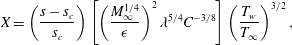 $$\begin{eqnarray}X=\left(\frac{s-s_{c}}{s_{c}}\right)\left[\left(\frac{M_{\infty }^{1/4}}{\unicode[STIX]{x1D716}}\right)^{2}\unicode[STIX]{x1D706}^{5/4}C^{-3/8}\right]\left(\frac{T_{w}}{T_{\infty }}\right)^{3/2},\end{eqnarray}$$
and,
 $$\begin{eqnarray}P=\left(\frac{p-p_{\infty }}{p_{\infty }}\right)\left[\left(\frac{M_{\infty }^{1/4}}{\unicode[STIX]{x1D716}}\right)^{2}\frac{\unicode[STIX]{x1D706}^{-1/2}C^{-1/4}}{\unicode[STIX]{x1D6FE}M_{\infty }^{2}}\right].\end{eqnarray}$$
For given free-stream conditions, wall temperatures and an unperturbed fully developed boundary layer, all the parameters inside the square brackets in (5.2) and (5.3) become constants so that the triple-deck theory suggests a universal curve seen in previous SBLI studies, and also shown to be experimentally valid by Lewis et al. (Reference Lewis, Kubota and Lees1968). However, in the presence of a leading edge separation, the boundary layer is growing under an adverse pressure gradient so that the Mach number,
 $\unicode[STIX]{x1D716}$
and
$\unicode[STIX]{x1D716}$
and
 $\unicode[STIX]{x1D706}$
are no longer constants, and even
$\unicode[STIX]{x1D706}$
are no longer constants, and even
 $C$
was seen to be varying slightly depending on the wall temperature. As noted earlier, separation pressures seem no longer independent of wall temperatures as has been the case of interactions with well-developed boundary layers prior to separation.
$C$
was seen to be varying slightly depending on the wall temperature. As noted earlier, separation pressures seem no longer independent of wall temperatures as has been the case of interactions with well-developed boundary layers prior to separation.

Figure 14. Deviation of the present data from the Blasius boundary layer in the triple-deck theory; (a,b) take into account the effects of varying flow conditions at the edge of the boundary layer with wall temperature as opposed to the standard triple-deck formulation.
The discrepancy in the scales of
 $X$
and
$X$
and
 $P$
between the present case and the SBLI with a prior well-developed boundary layer is illustrated in figure 14.
$P$
between the present case and the SBLI with a prior well-developed boundary layer is illustrated in figure 14.
 $a/a_{bl}$
represents the present values in the square brackets in (5.2) normalised by
$a/a_{bl}$
represents the present values in the square brackets in (5.2) normalised by
 $M_{\infty }$
,
$M_{\infty }$
,
 $Re_{\infty ,L_{e}}$
,
$Re_{\infty ,L_{e}}$
,
 $\unicode[STIX]{x1D706}$
and
$\unicode[STIX]{x1D706}$
and
 $C$
. Similarly, the parameter
$C$
. Similarly, the parameter
 $b/b_{bl}$
represents the deviation of
$b/b_{bl}$
represents the deviation of
 $P$
from the Blasius values. We immediately see that, firstly, the discrepancy in the
$P$
from the Blasius values. We immediately see that, firstly, the discrepancy in the
 $X$
scaling is much more than that of
$X$
scaling is much more than that of
 $P$
, as expected. We see that with moderate to no cooling (adiabatic), the discrepancy increases by more than a factor of 2 in the case of
$P$
, as expected. We see that with moderate to no cooling (adiabatic), the discrepancy increases by more than a factor of 2 in the case of
 $X$
. On the other hand, with the two coldest wall cases (where the boundary layer growth is considerably larger), the deviation is much less in the case of both
$X$
. On the other hand, with the two coldest wall cases (where the boundary layer growth is considerably larger), the deviation is much less in the case of both
 $X$
and
$X$
and
 $P$
. Another point to note is that the deviation in
$P$
. Another point to note is that the deviation in
 $P$
from the coldest to adiabatic wall is increased by nearly
$P$
from the coldest to adiabatic wall is increased by nearly
 $80\,\%$
.
$80\,\%$
.
6 Summary and conclusions
Hypersonic leading edge separation along with effects of wall temperature on separation have been studied numerically. Such a geometry was first used by Chapman et al. (Reference Chapman, Kuehn and Larson1958) to propose their isentropic recompression theory, which is shown to be generally valid at high Reynolds numbers and low Mach numbers with no pre-existing boundary layer. The present hypersonic results show that due to strong viscous effects, separation occurs not at the leading edge but slightly downstream of it (within 10 % of the distance from the leading edge) and shown to have strong dependence on wall temperature. The higher the wall temperature, the closer was the separation location to the leading edge. In all cases, however, there was a discernible growth of the boundary layer before interaction and separation. In the range of wall temperatures studied, the flow was mainly in the subcritical range (large Neiland number) and only in the case of adiabatic wall it was seen to be nearly transcritical (Neiland number of the order unity).
The existence of multiple vortices embedded in large separated flows, as previously seen in the investigations of Neiland and his co-researchers, has been verified. In the present investigation, the separated flow was found to consist of a main vortex and an embedded corner eddy. For colder wall temperatures, both the main vortex and the corner eddy were predominantly disposed towards the expansion surface. They migrated downstream towards the compression surface with increase in wall temperature. Another feature of the corner eddy found in this investigation was its double-loop nature which is attributed to the discontinuity at the vertex.
Although the hypersonic leading edge separation showed many features of free interaction, there were significant differences due to strong effect of the leading edge which inhibits the Blasius-type constant pressure boundary layer before interaction. These differences are accentuated with increase in wall temperature causing separation to move upstream towards the leading edge. These are highlighted and discussed. The study has clearly shown the need for more numerical studies as well as benchmark experimental data.
Acknowledgements
The authors are grateful to the Australian research Council for their support under grant (DP-140100842). They would also like to acknowledge National Facility Systems (NCI) for computer resources, and the US Office of Aerospace Research and Development (AOARD) for their support. Finally but by no means least, our sincere thanks are due to Professor G. Candler, of the University of Minnesota, for permission to use his US3D code for this investigation. We would like to thank the referees for their helpful comments and criticism, which have helped improve the paper.


