2.1. Linear models

For small-amplitude waves, the boundary conditions (2.1) can be linearized to

(2.2a,b)\begin{equation} \zeta_t=W_i, \quad {{\varPhi_i}_{t}} + g\zeta ={-}{P_i/\rho_i}. \end{equation}

Here, $\varPhi _i$ and $W_i$ can be approximated by those evaluated at the mean interface ($z=0$) so that $\varPhi _i (\boldsymbol x,t)\simeq \phi _i(\boldsymbol x,0,t) = \phi _{i_0}(\boldsymbol x,t)$ and $W_i(\boldsymbol x,t) \simeq \partial {\phi _i}/\partial z\vert _{z=0} =w_{i_0}(\boldsymbol x,t)$.

When the three-dimensional Laplace equations are solved for $\phi _i$ $(i=1,2)$ with the top and bottom boundary conditions given by $\partial \phi _1/\partial z\vert _{z=h_1} = 0$ and $\partial \phi _2/\partial z\vert _{z=-h_2} = 0$, respectively, their solutions can be written, in Fourier space, as

(2.3)\begin{equation} \hat{\phi}_i(\boldsymbol k,z,t)= \{\cosh [k(z+({-}1)^ih_i)]/\cosh(kh_i) \} \hat \phi_{i_0} (\boldsymbol k,t), \end{equation}

where $\hat f (\boldsymbol k,z,t)$ is the Fourier transform of $f(\boldsymbol x,z,t)$, $k=\vert \boldsymbol k\vert$ with $\boldsymbol k$ being the two-dimensional wavenumber vector and $h_1$ and $h_2$ are the thicknesses of the upper and lower layers, respectively. Then, from (2.3), one can obtain

(2.4)\begin{equation} \hat w_{i_0}(\boldsymbol k,t)=({-}1)^i(k\tanh kh_i) \hat \phi_{i_0}(\boldsymbol k,t), \end{equation}

from which the approximate expressions for $W_i\simeq w_{i_0}$ are given, in terms of $\varPhi _i\simeq \phi _{i_0}$, by

(2.5)\begin{equation} \hat W_i(\boldsymbol k,t)\simeq ({-}1)^i (k\tanh kh_i) \hat \varPhi_i(\boldsymbol k,t). \end{equation}

Finally, after taking the Fourier transform of (2.2) and using (2.5), the four linear equations for $\zeta$, $\varPhi _i$ ($i=1,2$) and $P$ are given, in Fourier space, by

(2.6a,b)\begin{equation} \hat \zeta_t=({-}1)^i(k\tanh kh_i) \hat \varPhi_i, \quad \hat \varPhi_{i_t }+ g\hat \zeta ={-}\hat P/\rho_i. \end{equation}

Assuming $(\hat \zeta, \hat \varPhi _i, \hat P) \sim \exp (-{\rm i}\omega t)$, the coupled system (2.6) yields the full linear dispersion relation for internal gravity waves (Lamb Reference Lamb1932)

(2.7)\begin{equation} \omega^2=\frac{(\rho_2-\rho_1)gk\tanh kh_1\tanh kh_2}{\rho_1 \tanh kh_2+\rho_2 \tanh kh_1}, \end{equation}

where the wave frequency $\omega$ is always real.

For long waves in shallow water with $kh_i\ll 1$ and $h_1/h_2=O(1)$, one can expand ${T_i}=\tanh kh_i$ as

(2.8)\begin{equation} {T}_i= \sum_{n=0}^\infty \frac{2^{2n+2}(2^{2n+2}-1)B_{2n+2}}{(2n+2)!} (kh_i)^{2n+1}, \end{equation}

where $B_{2n}$ are the Bernoulli numbers given by $B_0=1$, $B_2=1/6$, $B_4=-1/30$, $B_6=1/42$, $\cdots$.

When the upper limit for the summation in (2.8) is replaced by an integer $M\, (\ge 0)$, one can find a truncated linear system given, from (2.6), by

(2.9a,b)\begin{equation} \hat \zeta_t=({-}1)^i k{T}_{i,M} \hat \varPhi_i, \quad {\hat \varPhi}_{i_t}+ g\hat \zeta ={-}\hat P/\rho_i, \end{equation}

where ${T}_{i,M}$ represents the $M$th-order long-wave approximation of ${T}_i$ valid to $O(\beta ^{2M+1})$ with $kh_i=O(\beta )$. The linear dispersion relation of this truncated system can be found as

(2.10)\begin{equation} \omega^2=\frac{(\rho_2-\rho_1) gk T_{1,M} T_{2,M}}{\rho_1 T_{2,M} +\rho_2 T_{1,M}} . \end{equation}

For example, for $M=2$, the dispersion relation is given by

(2.11)\begin{equation} \omega^2=\frac{ (\rho_2-\rho_1) gk^2h_1h_2 [1-\frac{1}{3}(kh_1)^2+\frac{2}{15} (kh_1)^4][1-\frac{1}{3}(kh_2)^2+\frac{2}{15} (kh_2)^4]} {\rho_2h_1[1-\frac{1}{3}(kh_1)^2+\frac{2}{15} (kh_1)^4] +\rho_1h_2[1-\frac{1}{3}(kh_2)^2+\frac{2}{15} (kh_2)^4]}, \end{equation}

whose right-hand side is positive so that $\omega$ is always real. On the other hand, under the leading-order approximation ($M=1$), or by neglecting terms proportional to $(kh_i)^4$ in (2.11), its right-hand side becomes negative for large $k$ values. If this happens, $\omega$ is purely imaginary so that the system is unstable and its imaginary part represents the growth rate. In general, the system for the interface potentials $\varPhi _i$ is stable for even $M$ while that for odd $M$ is unstable. The same observation was made for surface waves in Choi (Reference Choi2022).

It should be stressed that this discussion about stability of the linear system (2.6) or its long-wave approximation (2.9) is limited to perturbations to the flat interface without background currents. When the interface is no longer flat, different horizontal velocities are induced in the top and bottom layers. Due to this velocity discontinuity across the interface, short-wavelength disturbances are expected to grow by the KH instability mechanism (Jo & Choi Reference Jo and Choi2002). As we are interested in large-amplitude internal waves, the stability of a deformed interface should be examined, but its analysis will be postponed until a high-order long-wave model is obtained.

Instead of the interface potentials, the long-wave model, such as the MCC model, is often written in terms of the layer-mean velocities $\bar {\boldsymbol u}_i$ defined by

(2.12a,b)\begin{equation} \bar{\boldsymbol u}_1=\frac{1}{(h_1-\zeta)}\int_{\zeta}^{h_1}\boldsymbol{\nabla} \phi_1\, {\rm d} z ,\quad \bar{\boldsymbol u}_2=\frac{1}{(h_2+\zeta)}\int_{{-}h_2}^{\zeta}\boldsymbol{\nabla} \phi_2\, {\rm d} z . \end{equation}

For small-amplitude waves, after replacing $\zeta$ by $0$ in the limit of the integration and using (2.3), the Fourier transforms of $\bar {\boldsymbol u}_i$ can be approximated by $\hat {\bar {\boldsymbol u}}_i \simeq -{\rm i} \boldsymbol k \tanh kh_i/(kh_i) \hat \varPhi _i$, from which we have $h_i \widehat {\boldsymbol {\nabla } \boldsymbol {\cdot} \bar {\boldsymbol u}_i} \simeq -k\tanh kh_i \hat {\varPhi }_i$. Then, from (2.9), the linear system for $\zeta$, $\bar {\boldsymbol u}_i$ and $P$ can be found, in Fourier space, as

(2.13a,b)\begin{equation} \hat \zeta_t = ({-}1)^{i+1} h_i\widehat{\boldsymbol{\nabla} \boldsymbol{\cdot} \bar{\boldsymbol u}_i}, \quad kh_i\coth kh_i \hat{\bar{\boldsymbol u}}_{i_t} +g\widehat{\boldsymbol{\nabla} \zeta}={-} \widehat{\boldsymbol{\nabla} P}/\rho_i. \end{equation}

Once again, for long waves, when truncated at $O(\beta ^{2M})$, the linear system (2.13) yields the following dispersion relation:

(2.14)\begin{equation} (\rho_1h_2 K_{1,M}+\rho_2 h_1K_{2,M})\omega^2=(\rho_2-\rho_1)gk^2h_1h_2, \end{equation}

where $K_{i,M}$ are the truncated series of $K_i=kh_i\coth kh_i$ given by

(2.15)\begin{equation} K_{i,M}=\left[1+\frac{1}{3}(kh_i)^2-\frac{1}{45}(kh_i)^4+\cdots +\frac{2^{2M}B_{2M}}{(2M)!} (kh_i)^{2M}\right] . \end{equation}

Contrary to the system for the surface velocity potentials $\varPhi _i$, the system for the layer-mean velocities $\bar {\boldsymbol u}_i$ is stable for odd $M$, but is unstable for even $M$.

To regularize the MCC model that is ill posed when the interface is deformed, Choi et al. (Reference Choi, Barros and Jo2009) used the velocity potentials at the top and bottom boundaries in the long-wave model. For small-amplitude waves, the interface potentials $\varPhi _i$ and the velocity potentials evaluated at the rigid top and bottom boundaries $\varphi _i (\boldsymbol x,t) =\phi _i(\boldsymbol x,z=(-1)^{i+1} h_i ,t)$ are related, from (2.3), as

(2.16)\begin{equation} \hat\varPhi_i\simeq \hat \phi_{i_0} (\boldsymbol k,t) =\cosh(kh_i) \hat\varphi_i (\boldsymbol k,t). \end{equation}

Then, from (2.6) with (2.16), the four linear equations for $\hat \zeta$, $\hat \varphi _i$ ($i=1,2$) and $\hat P$ can be obtained as

(2.17a,b)\begin{equation} \hat \zeta_t=({-}1)^i (k \sinh kh_i) \hat \varphi_i, \quad ( \cosh kh_i)\hat \varphi_{i_t }+ g\hat \zeta ={-}\hat P/\rho_i. \end{equation}

For $kh_i=O(\beta )\ll 1$, when the expansions for $C_i=\cosh kh_i$ and $S_i=\sinh kh_i$ are truncated at $O(\beta ^{2M})$, as before, the dispersion relation for (2.17) is given by

(2.18)\begin{equation} \omega^2=\frac{(\rho_2-\rho_1) gk S_{1,M}S_{2,M}}{\rho_1C_{1,M} S_{2,M}+\rho_2S_{1,M} C_{2,M}}, \end{equation}

where $C_{i,M}$ and $S_{i,M}$ are the truncated series of $C_i$ and $S_i$, respectively, given by

(2.19a)\begin{gather} C_{i,M}=\left [1+\frac{(kh_i)^2}{2!}+\cdots +\frac{(kh_i)^{2M}}{(2M)!}\right ] , \end{gather}

(2.19b)\begin{gather}S_{i,M}=kh_i\left [1+\frac{(kh_i)^2}{3!}+\cdots +\frac{(kh_i)^{2M}}{(2M+1)!}\right ]. \end{gather}

As the right-hand side of (2.18) is always positive for any values of $k$ and $M$, the wave frequency $\omega$ is always real. Unlike that for the interface velocity potentials $\varPhi _i$ or the layer-mean velocities $\bar {\boldsymbol u}_i$, the system for the top and bottom velocity potentials $\varphi _i$ given by (2.17) is stable, at any order of approximation, to all small disturbances on the flat surface. Therefore, the top and bottom velocity potentials $\varphi _i$ are chosen to write a high-order long-wave system.

2.2. Nonlinear models

Similarly to Choi (Reference Choi2022), we sketch briefly the derivation of a high-order long-wave model for $\varphi _i$. First we expand the three-dimensional velocity potentials $\phi _i(\boldsymbol x,z,t)$ $(i=1,2)$ in Taylor series about fixed vertical levels, or $z=z_{i_\alpha }$

(2.20)\begin{align} \phi_i(\boldsymbol x, z,t) &=\left.\sum_{j=0}^\infty \frac{({-}1)^j (z-z_{i_\alpha})^{2j}}{(2j)!}\nabla^{2j} \phi_i \right\vert_{z=z_{i_\alpha}}\nonumber\\ &\quad +\sum_{j=0}^\infty \frac{({-}1)^j (z-z_{i_\alpha})^{2j+1}}{ (2j+1)!}\nabla^{2j+1}\boldsymbol{\cdot}\nabla^{{-}1} \left. \frac{\partial \phi_i}{\partial z}\right\vert_{z=z_{i_\alpha}}. \end{align}

By introducing in (2.20)

(2.21a,b)\begin{equation} {{\phi_i}_{\alpha}}= \phi_i\vert_{z=z_{i_\alpha}},\quad {{w_i}_{\alpha}}= {\partial \phi_i/\partial z} \vert_{z=z_{i_\alpha}}, \end{equation}

$\phi _i(\boldsymbol x, z,t)$ and $w_i(\boldsymbol x, z,t)= {\partial \phi _i/\partial z}$ can be written (Madsen et al. Reference Madsen, Bingham and Liu2002; Choi Reference Choi2022) as

(2.22a)\begin{gather} \phi_i=\cos[(z-z_{i_\alpha}) \nabla] {{\phi_i}_{\alpha}} +\sin [(z-z_{i_\alpha}) \nabla] \boldsymbol{\cdot} \nabla^{{-}1} {{w_i}_{\alpha}}, \end{gather}

(2.22b)\begin{gather}w_i={-}\sin [(z-z_{i_\alpha}) \nabla]\boldsymbol{\cdot}\nabla{\phi_i}_\alpha +\cos [(z-z_{i_\alpha}) \nabla] {w_i}_\alpha. \end{gather}

For finite-amplitude long waves in shallow water, when we choose $z_{i_\alpha }=h_1$ and $-h_2$ for $i=1$ and $2$, respectively, (2.22) can be rewritten, with $w_{i_\alpha }=0$ at the flat top and bottom boundaries, as

(2.23a,b)\begin{equation} \phi_i(\boldsymbol x, z,t)=\cos[(z+({-}1)^i h_i) \nabla] \varphi_i,\quad w_i(\boldsymbol x, z,t)={-}\sin [(z+({-}1)^i h_i) \nabla]\boldsymbol{\cdot}\nabla \varphi_i, \end{equation}

where $\varphi _1(\boldsymbol x,t)$ and $\varphi _2(\boldsymbol x,t)$ are the velocity potentials evaluated at the top and bottom boundaries, respectively. When $z=\zeta$ is substituted into (2.23), $\varPhi _i$ and $W_i$ can be expressed, in terms of $\zeta$ and $\varphi _i$, as

(2.24a,b)\begin{equation} \varPhi_i=\cos [(\zeta+({-}1)^i h_i) \nabla] \varphi_i ,\quad W_i={-}\sin [(\zeta+({-}1)^i h_i) \nabla]\boldsymbol{\cdot}\nabla \varphi_i . \end{equation}

Then, substituting (2.24) into (2.1) yields formally a system of nonlinear evolution equations for $\zeta$ and $\varphi _i$ ($i=1,2$) along with an additional unknown $P$, although the cosine and sine functions in (2.24) need to be expanded in infinite series and, then, truncated to a certain order in $\beta ^2$ for practical applications, as discussed in § 3.

Once the high-order long-wave model for $\varphi _i$ is found, one can obtain a similar model for the interface velocity potentials $\varPhi _i$ or for the layer-mean velocities $\bar {\boldsymbol u}_i$ using the relationships between these variables, as shown in Appendices A and B. However, as mentioned previously, the long-wave model for $\varPhi _i$ or $\bar {\boldsymbol u}_i$ should be used with care as it is stable about the zero states only when truncated at even or odd orders in $\beta ^2$, respectively. Furthermore, when the interface is deformed, both models suffer from the KH instability.

3.1. Expansion in terms of the top and bottom velocity potentials

Following Choi (Reference Choi2022), by expanding the cosine and sine functions in (2.24), $\varPhi _i$ and $W_i$ can be expressed, in terms of $\zeta$ and $\varphi _i$, as

(3.1a,b)\begin{gather} \varPhi_i=\sum_{m=0}^\infty \varPhi_{i,{2m}} ,\quad \varPhi_{i,{2m}}= \frac{({-}1)^m}{(2m)!} \eta_i^{2m} \nabla^{2m} \varphi_i, \end{gather}

(3.2a,b)\begin{gather}W_i=\sum_{m=0}^\infty W_{i,{2m}} ,\quad W_{i,{2m}}=({-}1)^i \frac{({-}1)^{m+1}}{(2m+1)!} \eta_i^{2m+1} \nabla^{2(m+1)} \varphi_i , \end{gather}

where both $\varPhi _{i,{2m}}$ and $W_{i,{2m}}$ explicitly depend only on $\zeta$ and $\varphi _i$, and $\eta _i$ $(i=1,2)$ are defined by

(3.3)\begin{equation} \eta_i=h_i+({-}1)^i\zeta. \end{equation}

Assuming that $\eta _i \nabla =O(h_i/\lambda )=O(\beta )\ll 1$ with $\zeta /h_i=O(a/h_i)=O(\alpha )=O(1)$, one can notice that $\varPhi _{i,{2m}}/\varPhi _i=O(\beta ^{2m})$ and $W_{i,{2m}}/\vert \nabla \varPhi _i\vert =O(\beta ^{2m+1})$ for $m\ge 0$. Although no small parameter is explicitly introduced, these series can be considered asymptotic series in $\beta ^2$ when truncated.

3.2. System of nonlinear evolution equations

By substituting (3.1)–(3.2) into (2.1), the nonlinear evolution equations for $\zeta$, $P$ and $\varphi _i$ can be obtained as

(3.4a,b)\begin{equation} \zeta_t=\sum_{m=0}^\infty {\rm Q}_{i,{2m}}(\zeta,\varphi_i),\quad {{\varPhi_i}_{t}}={-}P/\rho_i+\sum_{m=0}^\infty {\rm R}_{i,{2m}}(\zeta,\varphi_i), \end{equation}

where $\varPhi _i$ are given, in terms of $\zeta$ and $\varphi _i$, by (3.1). In (3.4), ${\rm Q}_{i,{2m}}$ ($m\ge 0$) are given by

(3.5a)\begin{gather} {\rm Q}_{i,0}={-}\boldsymbol{\nabla}\zeta \boldsymbol{\cdot} \boldsymbol{\nabla} \varPhi_{i,0}+W_{i,0}, \end{gather}

(3.5b)\begin{gather}{\rm Q}_{i,{2m}}={-}\boldsymbol{\nabla}\zeta \boldsymbol{\cdot} \boldsymbol{\nabla} \varPhi_{i,{2m}}+W_{i,{2m}}+\vert\boldsymbol{\nabla} \zeta\vert^2 W_{i,{2(m-1)}}\quad \text{for } m\ge 1, \end{gather}

while ${\rm R}_{i,{2m}}$ ($m\ge 0$) are given by

(3.6a,b)$$\begin{gather} {\rm R}_{i,0}={-}g\zeta-\frac{1}{2}\vert\boldsymbol{\nabla} \varPhi_{i,0}\vert^2,\quad {\rm R}_{i,2}={-}\boldsymbol{\nabla} \varPhi_{i,0}\boldsymbol{\cdot} \boldsymbol{\nabla} \varPhi_{i,2} + \frac{1}{2}({W_{i,0}})^2, \end{gather}$$

(3.6c)$$\begin{gather}{\rm R}_{i,{2m}}={-}\frac{1}{2}\sum_{j=0}^{m} \boldsymbol{\nabla} \varPhi_{i,{2j}}\boldsymbol{\cdot} \boldsymbol{\nabla} \varPhi_{i,{2(m-j)}} +\frac{1}{2}\sum_{j=0}^{m-1}{W}_{i,{2j}}{W}_{i,{2(m-j-1)}}\nonumber\\ +\frac{1}{2}\vert\boldsymbol{\nabla} \zeta\vert^2\sum_{j=0}^{m-2}W_{i,{2j}} W_{i,{2(m-j-2)}} \quad \mbox{for $m\ge 2$} . \end{gather}$$

In (3.4), both $Q_{i,{2m}}$ and $R_{i,{2m}}$ are $O(\beta ^{2m})$ for $m\ge 0$.

When the expressions for $\varPhi _{i,{2m}}$ and $W_{i,{2m}}$ given by (3.1)–(3.2) are substituted into (3.5)–(3.6), one can find the explicit expressions of $Q_{i,{2m}}$ and $R_{i,{2m}}$ in terms of $\zeta$ and $\varphi _i$. In particular, it is useful to notice that ${\rm Q}_{i,{2m}}$ can be rewritten as

(3.7)\begin{equation} {\rm Q}_{i,{2m}}=({-}1)^i\boldsymbol{\nabla}\boldsymbol{\cdot}\left [\frac{({-}1)^{m+1}}{(2m+1)!} \eta_i^{2~m+1}\nabla^{2m}\boldsymbol{\nabla}\varphi_i\right ] \quad \text{for } m\ge 0. \end{equation}

As (3.4b) is the evolution equation for $\varPhi _i$, an additional step is necessary to find $\varphi _i$ from $\varPhi _i$. When the infinite series for $\varPhi _i$ in (3.1) are inverted, $\varphi _i$ can be expressed, in terms of $\zeta$ and $\varPhi _i$, as

(3.8a,b)\begin{gather} \varphi_i =\sum_{m=0}^\infty \varphi_{i,{2m}},\quad \varphi_{i,0}=\varPhi_i, \end{gather}

(3.8c)\begin{gather}\varphi_{i,{2m}}=\sum_{j=1}^m \frac{({-}1)^{j+1}}{(2j)!} \eta_i^{2j} \nabla^{2j} \varphi_{i,{2(m-j)}}\quad \text{for } m\ge 1. \end{gather}

3.3. Energy

After eliminating the pressure at the interface $P$, (3.4) can be rewritten as

(3.9a,b)\begin{equation} \zeta_t= \sum_{m=0}^\infty {\rm Q}_{2,{2m}}(\zeta,\varphi_2),\quad \varPsi_t=\sum_{i=1}^2({-}1)^i \rho_i \sum_{m=0}^\infty {\rm R}_{i,{2m}}(\zeta,\varphi_i), \end{equation}

along with

(3.10)\begin{equation} \sum_{m=0}^\infty {\rm Q}_{1,{2m}}(\zeta,\varphi_1) =\sum_{m=0}^\infty {\rm Q}_{2,{2m}}(\zeta,\varphi_2), \end{equation}

where $\varPsi$ is defined by

(3.11)\begin{equation} \varPsi=\rho_2\varPhi_2-\rho_1\varPhi_1. \end{equation}

In Benjamin & Bridges (Reference Benjamin and Bridges1997), it has been shown that the system given by (2.1) can be written as Hamilton's equations

(3.12a,b)\begin{equation} \zeta_t=\frac{\delta E }{\delta \varPsi},\quad \varphi_t={-}\frac{\delta E}{\delta \zeta}, \end{equation}

where $\delta E/\delta \zeta$ and $\delta E/\delta \varPsi$ represent the functional derivatives of the total energy $E$ with respect to $\zeta$ and $\varPsi$, respectively. Then, the system (3.12) conserves the total energy $E$ given by

(3.13)\begin{equation} E=\frac{1}{2} \int[ (\rho_2-\rho_1)g\zeta^2+\varPsi\zeta_t]\, {\rm d}\kern0.06em {\boldsymbol x} . \end{equation}

After substituting (3.4a) with (3.7) for $\zeta _t$ into (3.13) and using (3.11) for $\varPsi$ with (3.1) for the expressions for $\varPhi _i$, the total energy $E$ can be expanded as

(3.14)\begin{equation} E=\sum_{m=0}^\infty {E}_{2m} (\zeta,\varphi_1,\varphi_2),\end{equation}

where ${E}_{2m}=O(\beta ^{2m})$ for $m\ge 0$ are given by

(3.15a)\begin{gather} {E}_0=\frac{1}{2} \int [(\rho_2-\rho_1)g\zeta^2 +\rho_1\eta_1\boldsymbol{\nabla}\varphi_1\boldsymbol{\cdot} \boldsymbol{\nabla}\varphi_1+\rho_2\eta_2\boldsymbol{\nabla}\varphi_2\boldsymbol{\cdot} \boldsymbol{\nabla}\varphi_2]\, {\rm d}\kern0.06em {\boldsymbol x}, \end{gather}

(3.15b)\begin{gather}{E}_{2m}=\frac{1}{2} \sum_{i=1}^2 \sum_{j=0}^{m} \int \left [({-}1)^{i +m}\rho_i \frac{\eta_i^{2j+1}\nabla^{2j}(\boldsymbol{\nabla}\varphi_i)\boldsymbol{\cdot} \boldsymbol{\nabla} (\eta_i^{2(m-j)}\nabla^{2(m-j)}\varphi_i)} {(2j+1)!(2(m-j))!}\right ] \, {\rm d}\kern0.06em {\boldsymbol x} . \end{gather}

3.4. Truncated models

The infinite series on the right-hand sides of the system given by (3.4) need to be truncated for numerical computations. The governing equations for $\zeta$, $\varphi _i$ and $P$ correct to $O(\beta ^{2M})$ are then given by

(3.16a,b)\begin{gather} \zeta_t= \sum_{m=0}^M {\rm Q}_{i,{2m}}(\zeta,\varphi_i) ,\quad {{\varPhi_i}_{t}}={-}P/\rho_i+\sum_{m=0}^M {\rm R}_{i,{2m}}(\zeta,\varphi_i), \end{gather}

(3.16c)\begin{gather}\varPhi_i=\sum_{m=0}^M {\varPhi}_{i,{2m}}(\zeta,\varphi_i), \end{gather}

where ${\varPhi }_{i,{2m}}$, ${\rm Q}_{i,{2m}}$ and ${\rm R}_{i,{2m}}$ given by (3.1), (3.5) and (3.6), respectively, are all $O(\beta ^{2m})$. This system will be referred to as the $M$th-order system. As mentioned previously, after solving for $\varPhi _i$ (3.16b), $\varphi _i$ can be obtained from (3.16c), which can be inverted asymptotically, as shown in (3.8), or numerically using an iterative scheme introduced in Choi et al. (Reference Choi, Goullet and Jo2011). For a low-order approximation ($M=1$ or 2), the numerical approach is preferable as the asymptotic inversion is less accurate.

Under the small-amplitude assumption of $\zeta /h_i=O(a/h_i)\ll 1$, the truncated system (3.16) can be linearized to

(3.17a,b)\begin{equation} \zeta_t = ({-}1)^i {S}_{i,M}[\varphi_i],\quad {C}_{i,M}[{{\varphi_i}_{t}}]={-}P/\rho_i-g\zeta, \end{equation}

where the linear operators ${C}_{i,M}$ and ${S}_{i,M}$ are defined in (2.19). Notice that ${C}_{i,M} [\varphi _i ]$ and ${S}_{i,M} [\varphi _i ]$ are the linear approximations to $\varPhi _i$ and $W_i$. The linear dispersion relation for (3.17) is then given by (2.18), which shows that the wave frequency is always real for any choice of $k$ and $M$.

When the zeroth-order ($M=0$) approximation is made to (3.16), we have

(3.18a,b)\begin{equation} \zeta_t+({-}1)^{{-}i}\boldsymbol{\nabla}\boldsymbol{\cdot}(\eta_i\boldsymbol{\nabla}\varphi_i)=0,\quad {{\varphi_i}_{t}}+g\zeta +\tfrac{1}{2}\vert\boldsymbol{\nabla} \varphi_i\vert^2 ={-}P/\rho_i, \end{equation}

which are the (non-dispersive) shallow-water equations for a two-layer system.

3.4.1. First-order model

When the leading-order dispersive terms of $O(\beta ^2)$ are included, (3.16) can be reduced to the first-order ($M=1$) system given by

(3.19a)\begin{gather} \zeta_t +({-}1)^i\boldsymbol{\nabla}\boldsymbol{\cdot} \left [\left (\eta_i-\frac{\eta_i^3}{3!}\nabla^2\right )\boldsymbol{\nabla}\varphi_i\right ]=0, \end{gather}

(3.19b)\begin{gather}\left [ \left (1-\frac{\eta_i^2}{2!}\nabla^2\right )\varphi_i\right ]_t +g\zeta+\frac{1}{ 2}\boldsymbol{\nabla}\varphi_i\boldsymbol{\cdot} \boldsymbol{\nabla}\varphi_i ={-}\frac{P}{\rho_i}+ \boldsymbol{\nabla}\boldsymbol{\cdot}\left ( \frac{\eta_i^2} {2!}\nabla^2\varphi_i \boldsymbol{\nabla}\varphi_i\right ). \end{gather}

After taking the gradient, the first-order system (3.19) can be written, in terms of the bottom velocity $\boldsymbol v_i=\boldsymbol {\nabla }\varphi _i$, as

(3.20a)\begin{gather} \zeta_t +({-}1)^i\boldsymbol{\nabla}\boldsymbol{\cdot} \left [\left (\eta_i-\frac{\eta_i^3}{3!}\nabla^2\right )\boldsymbol v_i\right ]=0, \end{gather}

(3.20b)\begin{gather}\left[\boldsymbol v_i-\boldsymbol{\nabla} \left (\frac{\eta^2}{2!}\boldsymbol{\nabla}\boldsymbol{\cdot} \boldsymbol v_i\right )\right ]_t +\boldsymbol{\nabla} \left (g\zeta+\frac{1}{2}\boldsymbol v_i\boldsymbol{\cdot} \boldsymbol v_i\right ) ={-}\frac{P}{\rho_i}+\boldsymbol{\nabla} \left [\boldsymbol{\nabla}\boldsymbol{\cdot}\left \{ \frac{\eta_i^2}{2!} (\boldsymbol{\nabla}\boldsymbol{\cdot}\boldsymbol v_i) \boldsymbol v_i\right \}\right ]. \end{gather}

This is the regularized long-wave model of Choi et al. (Reference Choi, Barros and Jo2009) that is asymptotically equivalent to the strongly nonlinear long-wave model for the layer-mean velocities, or the MCC equations. Using the relationship between the bottom velocities $\boldsymbol v_i$ and the layer-mean velocities $\bar {\boldsymbol u}_i$ given, from (B2), by

(3.21)\begin{equation} \boldsymbol v_i = \bar{\boldsymbol u}_i+\frac{\eta_i^2}{3!}\nabla^2\bar{\boldsymbol u}_i+O(\beta^4), \end{equation}

one can show that the system given by (3.20) becomes the MCC equations for the layer-mean velocities $\bar {\boldsymbol u}_i$

(3.22a)\begin{gather} \zeta_t+({-}1)^i\boldsymbol{\nabla}\boldsymbol{\cdot} (\eta_i\bar{{\boldsymbol u}_{i}})=0, \end{gather}

(3.22b)\begin{gather}{\bar{{\boldsymbol u}_{i}}}_t+\bar{\boldsymbol u}_i\boldsymbol{\cdot}\nabla \bar{\boldsymbol u}_i+g\boldsymbol{\nabla}\zeta ={-}\frac{P}{\rho_i}+ \frac{1}{\eta_i}\nabla \left[\frac{\eta_i^3}{3}\{ \boldsymbol{\nabla}\boldsymbol{\cdot} {\bar{{\boldsymbol u}_i}_{t}} +\bar{\boldsymbol u}_i\boldsymbol{\cdot}\boldsymbol{\nabla} (\boldsymbol{\nabla}\boldsymbol{\cdot} \bar{{\boldsymbol u}_{i}})-(\boldsymbol{\nabla}\boldsymbol{\cdot} \bar{{\boldsymbol u}_{i}})^2\}\right ]. \end{gather}

Here, we have used $\nabla (\nabla \boldsymbol {\cdot} \bar {\boldsymbol u}_i)=\nabla ^2 \bar {\boldsymbol u}_i+O(\beta ^2)$ from $\nabla \times \bar {\boldsymbol u}_i=O(\beta ^2)$, which can be seen from (3.21).

3.4.2. Second-order model

The second-order ($M=2$) model correct to $O(\beta ^4)$ can be written explicitly, from (3.16), as

(3.23a)\begin{equation} \zeta_t +({-}1)^i\boldsymbol{\nabla}\boldsymbol{\cdot} \left [\left \{\eta_i-\frac{\eta_i^3}{3!}\nabla^2+ \frac{\eta_i^5} {5!}(\nabla^2)^2\right \}\boldsymbol{\nabla}\varphi_i\right ]=0, \end{equation}

(3.23b)\begin{align} &\left [ \left \{1-\frac{\eta_i^2}{2!}\nabla^2+\frac{\eta_i^4}{4!}(\nabla^2)^2\right \}\varphi_i\right ]_t +g\zeta+\frac{1}{2}\boldsymbol{\nabla}\varphi_i\boldsymbol{\cdot} \boldsymbol{\nabla}\varphi_i \nonumber\\ &\quad ={-}\frac{P}{\rho_i}+ \boldsymbol{\nabla}\boldsymbol{\cdot}\left ( \frac{\eta_i^2}{2!} \nabla^2\varphi_i \boldsymbol{\nabla}\varphi_i\right ) -\boldsymbol{\nabla}\boldsymbol{\cdot}\left [\frac{\eta_i^4}{4!} \boldsymbol{\nabla}\varphi_i (\nabla^2)^2 \varphi_i +\frac{\eta_i^4}{16} \boldsymbol{\nabla}(\nabla^2\varphi_i)^2\right ] . \end{align}

The total energy truncated at $O (\beta ^4 )$ is given by $E=E_0+E_2+E_4$ with $E_{2m}$ $(m=0,1,2)$ defined, from (3.14)–(3.15), by

(3.24a)\begin{gather} {E}_0=\frac{1}{2} \int [(\rho_2-\rho_1)g\zeta^2 +\rho_1\eta_1\boldsymbol{\nabla}\varphi_1\boldsymbol{\cdot} \boldsymbol{\nabla}\varphi_1+\rho_2\eta_2\boldsymbol{\nabla}\varphi_2\boldsymbol{\cdot} \boldsymbol{\nabla}\varphi_2]\, {\rm d}\kern0.06em {\boldsymbol x}, \end{gather}

(3.24b)\begin{gather}{E}_{2} =\frac{1}{3!} \sum_{i=1}^2 ({-}1)^{i}\rho_i \int\eta_i^3 [(\nabla^2\varphi_i)^2-\boldsymbol{\nabla} \varphi_i\boldsymbol{\cdot}\nabla^2\boldsymbol{\nabla}\varphi_i]\, {\rm d}\kern0.06em {\boldsymbol x}, \end{gather}

(3.24c)\begin{gather}E_4 =\frac{1}{5!} \sum_{i=1}^2 ({-}1)^i \rho_i \int \eta_i^5[3\nabla^2(\boldsymbol{\nabla}\varphi_i)\boldsymbol{\cdot} \nabla^2(\boldsymbol{\nabla}\varphi_i)\nonumber\\\hspace{38pt}-4(\nabla^4\varphi_i)(\nabla^2\varphi_i) +\boldsymbol{\nabla} \varphi_i\boldsymbol{\cdot}\nabla^4\boldsymbol{\nabla}\varphi_i ]\, {\rm d}\kern0.06em {\boldsymbol x}. \end{gather}

It should be mentioned that, unlike that for the surface velocity potentials or the layer-mean velocities, the truncated system given by (3.23) conserves the truncated total energy only asymptotically.

4.1. Wave profile

For one-dimensional travelling waves, after introducing $X=x-ct$ with $c$ being the solitary wave speed, (3.4a) with (3.7) can be integrated into

(4.1)\begin{equation} -c\zeta=({-}1)^i\sum_{m=0}^\infty \frac{({-}1)^{m+1}}{(2m+1)!} \eta_i^{2m+1}D^{2m}[v_i] \quad \text{for } m\ge 0, \end{equation}

where $D={{\rm d}/{\rm d} X}$ and $v_i(X)=D{\varphi _i}$. As the right-hand side of (4.1) is equivalent to $(-1)^{i+1}\eta _i {\bar u}_i$, it can be seen that we have imposed $(\zeta, {\bar u}_i)\to 0$ as $X\to -\infty$ to obtain (4.1).

Note that (4.1) can be inverted to find the expressions for $v_i$, in terms of $\zeta$, as

(4.2a,b)\begin{gather} v_i=\sum_{m=0}^\infty v_{i,{2m}}^s,\quad v_{i,0}^s=({-}1)^i \frac{c\zeta}{\eta_i}, \end{gather}

(4.2c)\begin{gather}v_{i,{2m}}^s=\sum_{j=1}^m \frac{({-}1)^{j+1}}{(2j+1)!}\eta_i^{2j} D^{2j}[v_{i,{2(m-j)}}^s] \quad m\ge 1. \end{gather}

Then, from (3.1)–(3.2), the new expressions for $\varPhi _i$ and $W_i$ can be found, in terms of $\zeta$, as

(4.3a,b)\begin{gather} \varPhi_i=\sum_{m=0}^\infty \varPhi^s_{i,{2m}} ,\quad \varPhi^s_{i,{2m}}=\sum_{j=0}^m \frac{({-}1)^j}{(2j)!} \eta_i^{2j} D^{2j-1} [v_{i,{2(m-j)}}^s] , \end{gather}

(4.4a,b)\begin{gather}W_i=\sum_{m=0}^\infty W^s_{i,{2m}},\quad W^s_{i,{2m}}=({-}1)^i \sum_{j=0}^m\frac{({-}1)^{j+1}}{(2j+1)!} \eta_i^{2j+1} D^{2j+1} [v_{i,{2(m-j)}}^s] . \end{gather}

After substituting these into the steady form of (3.4b) given by

(4.5)\begin{equation} -c\rho_i{\varPhi_i}_X={-}P+\rho_i\sum_{m=0}^\infty {\rm R}_{i,{2m}}^s(\zeta,\varphi_i), \end{equation}

and subtracting these two equations $(i=1,2)$ from each other to eliminate $P$, one can find an ordinary differential equation for $\zeta (X)$ as

(4.6a,b)\begin{equation} \sum_{i=1}^2 \sum_{m=0}^\infty ({-}1)^i\rho_i {\rm F}_{i,{2m}}(\zeta;c)=0, \quad {\rm F}_{i,{2m}}(\zeta;c)= cD[\varPhi^s_{i,{2m}}] + {\rm R}^s_{i,{2m}} , \end{equation}

where ${\rm F}_{i,{2m}}=O(\beta ^{2m})$ with ${\rm R}^s_{i,{2m}}$ given, from (3.6), by

(4.7a,b)\begin{gather} {\rm R}^s_{i,0}={-}g\zeta-\tfrac{1}{2}(D[\varPhi^s_{i,0}])^2,\quad {\rm R}^s_{i,2}={-}(D[\varPhi^s_{i,0}]) (D [\varPhi^s_{i,2}]) + \tfrac{1}{2} ({W^s_{i,0}})^2,\end{gather}

(4.7c)\begin{gather}{\rm R}^s_{i,{2m}}={-}\frac{1}{2} \sum_{j=0}^{m} (D[\varPhi^s_{i,{2j}}]) (D [\varPhi^s_{i,{2(m-j)}}] )+\frac{1}{2} \sum_{j=0}^{m-1}W^s_{i,{2j}}W^s_{i,{2(m-j-1)}}\nonumber\\ \hspace{-15pt}+\frac{1}{2} (D[\zeta])^2\sum_{j=0}^{m-2}W^s_{i,{2j}} W^s_{i,{2(m-j-2)}} \quad \text{for } m\ge 2 . \end{gather}

For $m=0,1,2$, the explicit expressions for ${\rm F}_{2,{2m}}$ in (4.6) are given by

(4.8a)\begin{gather} {\rm F}_{2,0}(\zeta;c) = \frac{1}{2} \zeta \left(\frac{2 c^2}{\eta_2}-\frac{c^2 \zeta}{\eta_2^2}-2g\right), \end{gather}

(4.8b)\begin{gather}{\rm F}_{2,2}(\zeta;c)= \frac{c^2 h_2^2}{6 \eta_2^2}(\zeta'^2 -2\eta_2\zeta''), \end{gather}

(4.8c)\begin{gather}{\rm F}_{2,4}(\zeta;c) ={-}\frac{c^2 h_2^2}{90 \eta_2^2} ( 12 \zeta'^4-48 \eta_2 \zeta'' \zeta'^2 +4\eta_2^2\zeta'''\zeta' +2\eta_2^3 \zeta'''' +3\eta_2^2 \zeta''^2 ). \end{gather}

The expressions for ${\rm F}_{1,{2m}}(\zeta ;c)$ ($m=0,1,2$) can be found from (4.8) by replacing $(g,\zeta,h_2)$ by $(-g,-\zeta,h_1)$.

After multiplying by $\zeta '$, (4.6) can be integrated once with respect to $X$ to have the following nonlinear ordinary differential equation

(4.9a,b)\begin{equation} \sum_{i=1}^2 \sum_{m=0}^\infty ({-}1)^i\rho_i {\rm N}_{i,{2m}}(\zeta;c)=0,\quad {\rm N}_{i,{2m}}(\zeta;c,h_i)=\int_{-\infty}^X {\rm F}_{i,{2m}}(\zeta;c)\zeta_{X'}\,{\rm d} X'. \end{equation}

Once again, the explicit expressions for ${\rm N}_{2,{2m}}$ ($m=0,1,2$) are given by

(4.10a)\begin{gather} {\rm N}_{2,0}(\zeta;c)=\frac{\zeta^2}{2\eta_2}(c^2-g\eta_2) , \end{gather}

(4.10b)\begin{gather}{\rm N}_{2,2}(\zeta;c)={-}\frac{c^2h_2^2}{6 \eta_2}{\zeta'^2}, \end{gather}

(4.10c)\begin{gather}{\rm N}_{2,4}(\zeta;c)={-}\frac{c^2 h_2^2}{90\eta_2} (2\eta_2^2 \zeta'\zeta''' -\eta_2^2 \zeta''^2+2\eta_2 \zeta'^2 \zeta''-12 \zeta'^4 ), \end{gather}

where we have imposed $\zeta ^{(n)}\to 0$ as $X\to -\infty$ for $n\ge 0$. Note that ${\rm N}_{1,{2m}}$ can be found by multiplying ${\rm N}_{2,{2m}}$ by -1 and replacing $(g,\zeta,\eta _2,h_2)$ by $(-g,-\zeta,\eta _1,h_1)$.

To find an asymptotic solitary wave solution, we expand $c$ and $\zeta$ as

(4.11a,b)\begin{equation} c=\sum_{m=0}^{\infty} c_{2m}, \quad \zeta=\sum_{m=0}^{\infty}\zeta_{2m}(X), \end{equation}

where both $c_{2m}$ and $\zeta _{2m}$ are assumed to be $O(\beta ^{2m})$. When these expansions are substituted into (4.9), the zeroth-order approximation, or $\sum _{i=1}^2(-1)^i \rho _i {\rm N}_{i,0}(\zeta ;c)=0$, yields a trivial solution, or $\zeta =0$ by imposing the zero boundary conditions at $X=-\infty$. This implies that $-\rho _1 {\rm N}_{1,0}(\zeta ;c)+\rho _2{\rm N}_{2,0}(\zeta ;c)=O(\beta ^2)$ and, therefore, one should include the $O(\beta ^2)$-terms for a non-trivial solution of (4.9).

4.1.1. First-order solution

The ordinary differential equation that appears at $O(\beta ^2)$ is given, from (4.9), by

(4.12)\begin{equation} \sum_{i=1}^2({-}1)^i\rho_i [{\rm N}_{i,0}(\zeta_0;c_0)+{\rm N}_{i,2}(\zeta_0;c_0) ]=0, \end{equation}

or

(4.13)\begin{equation} {\zeta_0'}^2=\frac{3\zeta_0^2 [(\rho_1\eta_{2_0}+\rho_2\eta_{1_0})c_0^2 -(\rho_2-\rho_1)g\eta_{1_0}\eta_{2_0}]}{ (\rho_1h_1^2\eta_{2_0}+\rho_2h_2^2\eta_{1_0})c_0^2}\equiv G(\zeta_0), \end{equation}

where $\zeta _0$ and $c_0$ will be referred to as the first-order solutions, and $\eta _{i_0}$ $(i=1,2)$ are defined by

(4.14)\begin{equation} \eta_{i_0}=h_i+({-}1)^i\zeta_0. \end{equation}

Equation (4.13) is the steady version of the MCC equations. From $\zeta _0'=0$ at $\zeta _0=a$, the leading-order wave speed $c_0$ and the amplitude $a$ are related (Choi & Camassa Reference Choi and Camassa1999) as

(4.15)\begin{equation} c_0^2= \frac{(\rho_2-\rho_1)g(h_1-a)(h_2+a)}{\rho_1(h_2+a)+\rho_2(h_1-a)}, \end{equation}

from which the linear long-wave speed $c_{lin}$ can be found, with $a=0$, as

(4.16)\begin{equation} c_{lin}^2=\frac{(\rho_2-\rho_1)g h_1 h_2}{\rho_1 h_2 +\rho_2 h_1}. \end{equation}

For the one-layer case with $\rho _1=0$, (4.13) can be reduced to

(4.17)\begin{equation} {\zeta_0'}^2=\left (\frac{3g}{c_0^2h_2^2}\right ) \zeta_0^2\left [\frac{c_0^2} {g}-(h_2+\zeta_0)\right ]. \end{equation}

As shown in Choi (Reference Choi2022), this is the first-order equation for solitary waves on the surface of a single layer of thickness $h_2$ first obtained by Rayleigh (Reference Rayleigh1876) and its solution is given by $\zeta (X)=a\,{\rm sech}^2(k_sX)$ and $c_0^2=g(h_2+a)$, where $(k_sh_2)^2=3a/[4(h_2+a)]$ with $a$ being the wave amplitude.

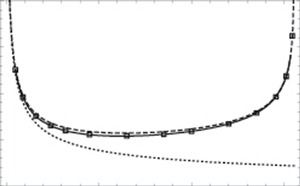
It was shown in Choi & Camassa (Reference Choi and Camassa1999) that the width of the internal solitary wave solution increases with the wave amplitude and a front solution appears at the maximum amplitude $a_m$ satisfying

(4.18a,b)\begin{equation} \rho_1(h_2+a_m)^2=\rho_2(h_1-a_m)^2,\quad \text{or, explicitly,}\quad a_{m}=\frac{ h_1\sqrt{\rho_2/\rho_1}- h_2}{\sqrt{\rho_2/\rho_1}+1}, \end{equation}

for which the maximum wave speed is given, from (4.10c), by

(4.19)\begin{equation} c_{m}^2=g( h_1+ h_2) \left (\frac{\sqrt{\rho_2/\rho_1}-1}{\sqrt{\rho_2/\rho_1}+1}\right ). \end{equation}

Note that the front solution for $a=a_m$ represents a heteroclinic orbit that connects two fixed points of (4.13) located at $\zeta _0=0$ and $a_m$.

4.1.2. Second-order solution

By substituting (4.11) into (4.9) and collecting terms of $O(\beta ^{2m})$, one can find an equation for $\zeta _{2m}$ $(m\ge 1)$ as

(4.20)\begin{equation} f_{1}(X)\zeta_{2m}' +f_{2}(X)\zeta_{2m}= f_{3}(X)c_{2m}+f_4(X), \end{equation}

where $f_4$ is a known function of $\zeta _{2l}$ and $c_{2l}$ $(l=0,1,\ldots, m-1)$ while $f_j$ ($j=1,2,3$), depending only on the leading-order solutions ($\zeta _0$ and $c_0$), are given by

(4.21a–c)\begin{equation} f_1=\sum_{i=1}^2 ({-}1)^i \rho_i \left. \frac{\partial {\rm N}_{i}}{\partial \zeta'}\right\vert_{0},\quad f_2=\sum_{i=1}^2 ({-}1)^i \rho_i \left. \frac{\partial {\rm N}_{i}}{\partial \zeta}\right\vert_0,\quad f_3=\sum_{i=1}^2 ({-}1)^i \rho_i \left. \frac{\partial {\rm N}_{i}}{\partial c}\right\vert_0, \end{equation}

with ${\rm N}_i={\rm N}_{i,0}+{\rm N}_{i,2}$ and subscript $0$ representing evaluation at $(\zeta,c)=(\zeta _0,c_0)$. Using (4.10a)–(4.10b) for ${\rm N}_{2,0}$ and ${\rm N}_{2,2}$ and the similar expressions for ${\rm N}_{1,0}$ and ${\rm N}_{1,2}$, one can find explicitly the following expressions for $f_j$ ($j=1,2,3$)

(4.22a)\begin{equation} {\zeta_0'}f_1 ={-}\zeta_0^2[( \rho_1\eta_{2_0}+\rho_2\eta_{1_0} )c_0^2-(\rho_2-\rho_1)g\eta_{1_0}\eta_{2_0} ] , \end{equation}

(4.22b)\begin{align} f_2&={-}\tfrac{1}{6}c_0^2(\rho_1h_1^2-\rho_2h_2^2) G(\zeta_0) +c_0^2(\rho_1h_2+\rho_2h_1)\zeta_0-\tfrac{3}{2}c_0^2(\rho_2-\rho_1)\zeta_0^2 \nonumber\\ &\quad -(\rho_2-\rho_1)gh_1h_2\zeta_0+\tfrac{3}{2}(\rho_2-\rho_1)g(h_2-h_1)\zeta_0^2 +2(\rho_2-\rho_1)g\zeta_0^3, \end{align}

(4.22c)\begin{equation} f_3 ={-}(\rho_2-\rho_1)g\eta_{1_0}\eta_{2_0}\zeta_0^2/c_0. \end{equation}

The solution of (4.20) is formally given by

(4.23a,b)\begin{equation} \zeta_{2m}=\frac{1}{f_{0}}\int_0^X f_{0}\left (\frac{f_{3}}{f_{1}}c_2 +\frac{f_4}{f_{1}}\right ){\rm d} X' +\frac{C}{f_0},\quad f_{0}(X)=\exp\left [\int(f_{2}/f_{1})\, {\rm d} X \right ], \end{equation}

where the integrating factor $f_0$ can be found, from (4.23b) with (4.22), as

(4.24)\begin{equation} f_0 ={1/ \zeta_0'} . \end{equation}

As the solitary wave is assumed to be an even function decaying to zero as $X\to \pm \infty$ (except for $a=a_m$, for which the front solution is found), the homogeneous solution of (4.20) given by $C\zeta _0'$ is an odd function decaying at infinities and will be therefore neglected. Note that $X=0$ is chosen for the lower limit of the integration in (4.23a). With this choice, $\zeta _{2m}$ are always zero at $X=0$ and the solitary wave amplitude $a$ remains unchanged with the order of approximation.

At $O(\beta ^2)$, the expression for $f_4$ that depends on $\zeta _0$ and $c_0$ is given by

(4.25)\begin{equation} f_4=[\rho_1N_{1_4}(\zeta_0,c_0)-\rho_2N_{2_4}(\zeta_0,c_0) ]\eta_{1_0}\eta_{2_0}, \end{equation}

where $N_{i_4}$ are given by (4.10c) for $i=2$ and the similar expression for $i=1$, as explained previously. In evaluating $f_4$, the following expressions for the derivatives of $\zeta _0$ would be useful

(4.26a–c)\begin{equation} {\zeta_0'}^2=G(\zeta_0),\quad \zeta_0''=\tfrac{1}{2}G'(\zeta_0),\quad \zeta_0'''=\tfrac{1}{2} \zeta_0' G'' (\zeta_0) , \end{equation}

where $G'(\zeta _0)={{\rm d} G/{\rm d}\zeta _0}$ and $G''(\zeta _0)={{\rm d}^2 G/{\rm d}\zeta _0^2}$ with $G(\zeta _0)$ defined by (4.13). Unlike the surface wave case in Choi (Reference Choi2022), this expression for $f_4$ is so complex that (4.23a) needs to be evaluated numerically.

After rewriting (4.23) with $C=0$ and ${\rm d} \zeta _0=\zeta _0'\,{\rm d} X$ as

(4.27)\begin{equation} \zeta_{2m}=\frac{1}{f_{0}}\int_a^{\zeta_0} f_{0} \left (\frac{f_{3}}{f_{1}}{c_2} + \frac{f_4}{f_{1}}\right )\frac{{\rm d}\zeta_0}{{\zeta_0'}} , \end{equation}

we first determine $c_2$ by removing the (non-integrable) singularity of the integrand at the lower limit, or $\zeta _0= a$. From the following asymptotic behaviour of the integrand near $\zeta _0=a$

(4.28)\begin{equation} \left (\frac{f_{0} f_{3}}{{\zeta_0'} f_{1}}, \frac{f_{0} f_4}{{\zeta_0'} f_{1}}\right ) =\frac{({\mu_1},\nu_1)}{|\zeta_0-a |^{3/2}} +\frac{({\mu_2},\nu_2)}{| \zeta_0-a |^{1/2}}+O(|\zeta_0-a|^{1/2}), \end{equation}

with $\mu _j$ and $\nu _j$ $(j=1,2)$ being constants, the leading-order singularity at $\zeta _0=a$ can be removed by choosing $c_2$ to be $c_2=-{\nu _1}/{\mu _1}$, which can be found explicitly as

(4.29)\begin{equation} \frac{c_2}{c_0}={-}\frac{a^2(\rho_1 h_1^2\eta_{1_a}+\rho_2 h_2^2\eta_{2_a}) (\rho_1\eta_{2_a}^2-\rho_2 \eta_{1_a}^2)^2} {40\eta_{1_a}\eta_{2_a}(\rho_1\eta_{2_a}+\rho_2\eta_{1_a}) (\rho_1h_1^2\eta_{2_a}+\rho_2h_2^2\eta_{1_a})^2}, \end{equation}

where $\eta _{i_a}=h_i+(-1)^ia$ ($i=1,2$). As $\rho _1\to 0$, this can be reduced to the result for surface waves on a single layer with the thickness $h_2$ (Choi Reference Choi2022)

(4.30)\begin{equation} \frac{c_2}{c_0}={-}\frac{a(h_2+a)}{40 h_2^2}\gamma, \end{equation}

where $c_0=[g(h_2+a)]^{1/2}$ and $\gamma =a/(h_2+a)$ is the smallness parameter used in the expansion.

Notice that $c_2$ in (4.29) vanishes at the maximum wave amplitude $a=a_m$, for which $\rho _1\eta _{2_a}^2-\rho _2 \eta _{1_a}^2=0$. This implies that the maximum wave speed predicted by the first-order (MCC) equations is indeed the exact solution of the Euler equations, as shown in Choi & Camassa (Reference Choi and Camassa1999). Although no correction to the wave speed $c_0$ at $a=a_m$ is necessary so that $c_{2m}=0$, the corresponding MCC solution for the wave profile is different from the exact solution of the Euler equations, in particular, in the transition region between the two constant states ($\zeta =0$ and $\zeta =a_m$).

Figure 2 shows the variation of the wave speed $c$ with the amplitude $\vert a\vert$ for the density and depth ratios given by $\rho _2/\rho _1= 1.022$ and $h_2/h_1=4.132$, respectively. These physical parameters were used to compute the solitary wave profiles in Camassa et al. (Reference Camassa, Choi, Michallet, Rusas and Sveen2006) to validate the MCC solution with the numerical solution of the Euler equations for the shallow configuration. The improvement for the wave speed by the second-order solution is relatively small as the first-order MCC solution $c_0$ given by (4.10c) predicts well the wave speed for the entire range of wave amplitudes, $0\le \vert a\vert \le \vert a_{m}\vert$, where the maximum amplitude $a_m/h_1$ is approximately $-$1.552. Nevertheless, one can see that the first-order solution slightly overpredicts the wave speed, and the second-order solution $c=c_0+c_2+O(\beta ^4)$ with $c_2$ given explicitly by (4.29) clearly improves the comparison with the Euler solution.

Figure 2. Solitary wave speed $c$ vs amplitude $\vert a\vert$. The second-order (solid line) solution $c=c_0+c_2+O(\beta ^4)$ is compared with the Euler solution (Camassa et al. Reference Camassa, Choi, Michallet, Rusas and Sveen2006) (open squares) and the first-order solution (dashed line) $c=c_0+O(\beta ^2)$, where $c_0$ and $c_2$ are given by (4.10c) and (4.29), respectively. Here, $c_{lin}$ is the linear wave speed given by (4.11a,b), the density and depth ratios are given by 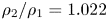$\rho _2/\rho _1= 1.022$ and $h_2/h_1=4.132$, respectively, and the maximum amplitude is $\vert a_m\vert /h_1\simeq 1.552$.

To find $\zeta _2$, (4.27) with $c_2$ given by (4.29) needs to be computed numerically. To accurately evaluate the integral, we rewrite (4.27) as

(4.31a)\begin{gather} \zeta_{2}=\frac{1}{f_{0}}\left [ 2(\mu_2c_2+\nu_2)\sqrt{\vert\Delta a\vert}+ \int_{a-\Delta a}^{\zeta_0} F(z) \,{{\rm d} z}\right ] , \end{gather}

(4.31b)\begin{gather}F(\zeta_0)= \frac{f_{0}}{{\zeta_0'}} \left (\frac{f_{3}}{f_{1}}{c_2} + \frac{f_4}{f_{1}}\right ) , \end{gather}

where the first term is $O(\vert \Delta a\vert ^{1/2})$ and represents the (approximate) evaluation of the integral from $z=a$ to $z=a-\Delta a$ with $\vert \Delta a/a\vert \ll 1$, where $\Delta a$ is a small shift away from a (integrable) singularity at $z=a$. The integration in (4.31a) is evaluated numerically with $\vert \Delta a\vert /h_1=10^{-10}$ using an integration routine ‘NIntegrate’ in the Mathematica (Wolfram Research, Inc., v.12). The computed $\zeta _2$ as a function of $\zeta _0$ is shown in figure 3 for four different wave amplitudes. Similarly to the wave speed, the second-order correction is still small. For $\vert a\vert /h_1=0.36$, 0.65 and 1.23, as $\zeta _2$ is positive while $\zeta _0$ is negative for solitary waves of depression, the second-order solution would lie above the first-order solution except for $\zeta _0=0$ and $\zeta _0=a$, where $\zeta _2=0$. On the other hand, for $\vert a\vert /h_1=1.51$ close to the maximum wave amplitude, $\zeta _2$ is positive for smaller values of $\vert \zeta _0\vert$, but is negative near the maximal displacement at $\zeta _0=a$.

Figure 3. Numerical evaluation of (4.27) for $\zeta _2$ parameterized by $\zeta _0$ for four different solitary wave amplitudes of depression: $\vert a\vert /h_1=0.36$ (dotted), 0.65 (dashed); 1.23 (dot-dashed); 1.51 (solid). Here, the density and depth ratios are given by $\rho _2/\rho _1= 1.022$ and $h_2/h_1=4.132$, respectively.

The computed second-order wave profiles given by $\zeta =\zeta _0+\zeta _2+O(\beta ^4)$ for $\vert a\vert /h_1=0.36, 0.65, 1.23, 1.51$ are shown in figure 4 and are indistinguishable from the Euler solutions. As shown in Choi & Camassa (Reference Choi and Camassa1999) and Camassa et al. (Reference Camassa, Choi, Michallet, Rusas and Sveen2006), the first-order MCC solutions are close to the Euler solutions over a wide range of wave amplitudes, but the improvement made by $\zeta _2$ can be clearly seen for intermediate wave amplitudes.

Figure 4. Comparison of internal solitary wave profiles for four different wave amplitudes: (a) $a/h_1=-0.36$; (b) $-$0.65; (c) $-$1.23; (d) $-$1.51. The second-order solitary wave solution (solid) given by $\zeta =\zeta _0+\zeta _2+O(\beta ^4)$ is compared with the Euler solution (Camassa et al. Reference Camassa, Choi, Michallet, Rusas and Sveen2006) (open squares), the first-order (MCC) solution $\zeta _0$ (dashed) and the weakly nonlinear (Koretweg–de Vries, KdV) solution (dotted). Here, the density and depth ratios are given by $\rho _2/\rho _1= 1.022$ and $h_2/h_1=4.132$, respectively.

Figure 5 shows the effective wavelength $\lambda$ defined by

(4.32)\begin{equation} \lambda= \left \vert \frac{1}{a} \int_0^\infty \zeta(X) \,{\rm d} X \right \vert =\lambda_0+\lambda_2+O(\beta^4), \end{equation}

where $\lambda _{2m}$ ($m=0,1$) are given by

(4.33)\begin{equation} \lambda_{2m}= \left \vert \frac{1}{a} \int_a^0 {\zeta_{2m}}({\rm d} \zeta_0/\zeta_0') \right \vert. \end{equation}

While $\lambda _0$ can be explicitly expressed in terms of complete elliptic functions, as shown in Choi & Camassa (Reference Choi and Camassa1999), $\lambda _2$ needs to be computed numerically. Using (4.27) and (4.33) for $m=1$, the expression for $\lambda _2$ can be obtained as

(4.34)\begin{equation} \lambda_{2}=\left \vert \frac{1}{a} \int_a^0 \int_a^{\zeta_0} F(z) \,{\rm d} z\,{\rm d} \zeta_0 \right \vert, \end{equation}

where $F(z)$ is given by (4.31b) with $f_0=1/\zeta _0'$. Once again, the ‘NIntegrate’ routine in the Mathematica has been used to evaluate the integration in (4.34).

Figure 5. Effective wavelength $\lambda$ vs wave amplitude $\vert a\vert$. The second-order solution (solid) is compared with the Euler solution (Camassa et al. Reference Camassa, Choi, Michallet, Rusas and Sveen2006) (open squares), the first-order (MCC) solution (dashed) and the weakly nonlinear (KdV) solution (dotted). Here, the density and depth ratios are given by $\rho _2/\rho _1= 1.022$ and $h_2/h_1=4.132$, respectively.

As observed in the comparison for the wave profiles, the second-order solution is expected to better predict the effective wavelength $\lambda$, particularly for intermediate wave amplitudes. As shown in figure 5, the second-order solution indeed agrees well with the Euler solution for the entire range of wave amplitudes, $0\le \vert a\vert \le \vert a_m\vert$. Therefore, for long internal waves in the shallow-water configuration, the second-order long-wave solution is expected to be sufficient and no higher-order approximation seems to be necessary for practical applications.

4.2. Velocity field induced by a solitary wave

The horizontal and vertical velocities, $(u_i,w_i)=({\phi _i}_X, {\phi _i}_z)$, induced by a solitary wave can be computed, from (2.23), as

(4.35a)\begin{gather} u_i(X, z)=\sum_{m=0}^\infty \frac{({-}1)^m}{(2m)!} [ z+({-}1)^ih_i ]^{2m} D^{2m} v_i, \end{gather}

(4.35b)\begin{gather}w_i(X, z)=\sum_{m=0}^\infty \frac{({-}1)^{m+1}}{(2m+1)!} [ z+({-}1)^i h_i ]^{2m+1} D^{2m+1} v_i, \end{gather}

where $\zeta \le z\le h_1$ for $i=1$ and $-h_2\le z\le \zeta$ for $i=2$. To find the asymptotically consistent velocity field, the top and bottom velocities $v_i(X)={\varphi _i}_X$ should be first expanded as

(4.36)\begin{equation} v_i=\sum_{m=0}^\infty v_{i,{2m}}^s, \end{equation}

where $v_{i,{2m}}^s=O(\beta ^{2m})$ can be found by substituting into (4.2) the expansions for $\zeta$ and $c$ given by (4.11). After substituting (4.36) into (4.35), one can find the following expressions of $u_i$ and $w_i$

(4.37a,b)\begin{gather} u_i(X,z)=\sum_{m=0}^\infty u_{i,{2m}}^s(X,z),\quad u_{i_{2m}}^s=\sum_{j=0}^m \frac{({-}1)^j} {(2j)!} [z+({-}1)^ih_i]^{2j} D^{2j} v_{i,{2(m-j)}}^s, \end{gather}

(4.38a)\begin{gather}w_i(X,z)=\sum_{m=0}^\infty w_{i,{2m}}^s(X,z), \end{gather}

(4.38b)\begin{gather}w_{i,{2m}}^s=\sum_{j=0}^m \frac{({-}1)^{j+1}} {(2j+1)!} [z+({-}1)^ih_i ]^{2j+1} D^{2j+1} v_{i,{2(m-j)}}^s, \end{gather}

where $u_{i,{2m}}^s$ and $w_{i,{2m}}^s$ are both $O(\beta ^{2m})$.

With the following expressions for $v_{i,{2m}}^s$ ($m=0,1$)

(4.39a)\begin{gather} v_{i,0}^s =({-}1)^i \frac{c_0\zeta_0}{\eta_{i_0}}, \end{gather}

(4.39b)\begin{gather}v_{i,2}^s= c_0 \left [({-}1)^i \left (\frac{c_2}{c_0}\frac{\zeta_0}{\eta_{i_0}}+\frac{h_i\zeta_2}{\eta_{i_0}^2}\right ) +\frac{\eta_{i_0}^2}{6} \left ( \frac{h_i\eta_{i_0}''} {\eta_{i_0}^2}-\frac{2h_i{\eta_{i_0}'}^2} {\eta_{i_0}^3}\right )\right ], \end{gather}

the horizontal velocity of the $i$th layer $u_i$ correct to $O(\beta ^2)$ is given explicitly by

(4.40)\begin{align} u_i(X,z)&=c_0 \left [({-}1)^i\left (\frac{\zeta_0}{\eta_{i_0}}+\frac{c_2} {c_0}\frac{\zeta_0}{\eta_{i_0}}+\frac{h_i\zeta_2}{\eta_{i_0}^2}\right ) \right.\nonumber\\ &\quad \left.+ \left (\frac{\eta_{i_0}^2}{6}-\frac{(z+({-}1)^ih_i)^2}{2}\right ) \left ( \frac{h_i\eta_{i_0}''}{\eta_{i_0}^2}-\frac{2h_i{\eta_{i_0}'}^2}{\eta_{i_0}^3}\right )\right ], \end{align}

where the expressions for $c_{2m}$ and $\zeta _{2m}$ ($m=0,1$) have been found in § 4.1.

Figure 6 shows the horizontal velocities $u_i$ at $X=0$ (at the location of the maximal displacement) given by

(4.41)\begin{equation} u_i(0,z)=\left. ({-}1)^i c_0 \left [\frac{\zeta_0}{ \eta_{i_0}}+\frac{c_2}{c_0}\frac{\zeta_0}{\eta_{i_0}} + \left (\frac{\eta_{i_0}^2} {6}-\frac{(z+({-}1)^ih_i)^2}{2}\right ) \left ( \frac{h_i\zeta_{0}''}{\eta_{i_0}^2}\right )\right ]\right\vert_{X=0}, \end{equation}

where $\zeta _2=\zeta _0'=0$ at $X=0$ have been used and $\zeta _0''$ can be computed, from (4.26b), as $\zeta _0''=G'[\zeta _0]/2$. Here, to better represent the variation in the vertical $z$ direction, note that $\vert u_i\vert$ are shown. Again, the second-order solution agrees well with the Euler solution for all wave amplitudes. As discussed previously, the correction $c_2$ to the leading-order wave speed $c_0$ is so small that the second term proportional to $c_2$ in (4.39b) is negligible. Therefore, the expressions for $u_i(0,z)$ without the second term used in Camassa et al. (Reference Camassa, Choi, Michallet, Rusas and Sveen2006) are good approximations to the second-order solution although they are asymptotically inconsistent.

Figure 6. Comparison of $\vert u_i(0,z)\vert$ for four different wave amplitudes: (a) $a/h_1=-0.36$; (b) $-$0.65; (c) $-$1.23; (d) $-$1.51. The second-order solitary wave solution (solid) given by (4.39a) is compared with the Euler solution (Camassa et al. Reference Camassa, Choi, Michallet, Rusas and Sveen2006) (open squares) and the mean velocity $\vert u_i\vert =\vert v_{i_0}^s \vert$ (dotted). Notice that $u_1=\vert u_1\vert$ and $u_2=-\vert u_2\vert$ for solitary waves propagating to the right. Here, the density and depth ratios are given by $\rho _2/\rho _1= 1.022$ and $h_2/h_1=4.132$, respectively.

The maximum horizontal velocity jump across the interface occurs at the location of the maximal displacement, or $X=0$, and can be found, from (4.39b) with $z=a$, as

(4.42)\begin{equation} U_2-U_1=(c_0+c_2)\frac{a(h_1+h_2)}{(h_1-a)(h_2+a)}-\frac{c_0}{6}G'(a)(h_1+h_2), \end{equation}

where $U_i=u_i(0,a)$. As shown in figure 7, the velocity jump for the second-order solitary wave solution is slightly greater than that for the first-order solution. Due to this increased velocity jump, the second-order internal solitary wave could be more unstable by the KH instability mechanism (Jo & Choi Reference Jo and Choi2002) and its stability needs to be examined when it is perturbed by short-wavelength disturbances.

Figure 7. The velocity jump across the interface $\vert U_2-U_1\vert$ vs the wave amplitude $\vert a\vert$: The second-order solution (solid) is compared with the first-order (MCC) solution (dashed) for the density and depth ratios given by $\rho _2/\rho _1= 1.022$ and $h_2/h_1=4.132$, respectively.