


1. Introduction
Gravity currents occur when a dense fluid propagates mostly horizontally in a relatively lighter fluid, under the effect of gravity. They are ubiquitous in air and water bodies and can be caused by a variety of geophysical processes that most often involve density changes due to temperature, salinity or dense suspended particulate matter. Turbidity currents, a type of gravity current in which the density difference is due to the presence of suspended sediment in a carrier fluid, are the main contributors to sediment transport in the world's oceans (Meiburg & Kneller Reference Meiburg and Kneller2010). As a result, both gravity and turbidity currents have been extensively studied over the past century (von Kármán Reference von Kármán1940; Benjamin Reference Benjamin1968; Huppert Reference Huppert1982; Härtel, Meiburg & Necker Reference Härtel, Meiburg and Necker2000b; Necker et al. Reference Necker, Härtel, Kleiser and Meiburg2002; Cantero et al. Reference Cantero, Lee, Balachandar and Garcia2007; Meiburg & Kneller Reference Meiburg and Kneller2010; Wells & Dorrell Reference Wells and Dorrell2021). Because of its simplicity, repeatability and reproducibility, the instantaneous lock-release of a dense fluid initially separated from the relatively lighter fluid by a removable gate has been the canonical and almost systematically considered configuration for the study of gravity currents, in laboratory experiments (e.g. Huppert & Simpson Reference Huppert and Simpson1980; Shin, Dalziel & Linden Reference Shin, Dalziel and Linden2004), numerical simulations (e.g. Härtel et al. Reference Härtel, Meiburg and Necker2000b; Meiburg, Radhakrishnan & Nasr-Azadani Reference Meiburg, Radhakrishnan and Nasr-Azadani2015) as well as analytical works (e.g. Benjamin Reference Benjamin1968; Holyer & Huppert Reference Holyer and Huppert1980; Ungarish Reference Ungarish2005; Tan et al. Reference Tan, Nobes, Fleck and Flynn2011; Flynn, Ungarish & Tan Reference Flynn, Ungarish and Tan2012; Khodkar, Nasr-Azadani & Meiburg Reference Khodkar, Nasr-Azadani and Meiburg2018; Zemach et al. Reference Zemach, Ungarish, Martin and Negretti2019). Many variants to the basic configuration have been used, for instance to study the role of the release depth and lock-length on the spreading of a gravity current from an axisymmetric lock-release, the spreading of three-dimensional gravity currents in a lock-exchange configuration with a partial-width lock (La Rocca et al. Reference La Rocca, Adduce, Sciortino and Pinzon2008) or the propagation of a rectilinear gravity current in the presence of a uniform flow (Hallworth, Hogg & Huppert Reference Hallworth, Hogg and Huppert1998; Cantero et al. Reference Cantero, Lee, Balachandar and Garcia2007). Gravity currents produced by constant and variable flux inflows have additionally been studied in a variety of configurations (Hogg et al. Reference Hogg, Nasr-Azadani, Ungarish and Meiburg2016; Longo et al. Reference Longo, Ungarish, Di Federico, Chiapponi and Addona2016). The continuous release of a dense scalar from a moving source has, to the best of our knowledge, never been studied systematically and no canonical configuration exists for the study of the resulting gravity current. The related problem of buoyant plumes or jets released in cross-flows has been investigated to a degree in engineering applications (Roberts Reference Roberts1979; Choi & Lee Reference Choi and Lee2007; Taherian & Mohammadian Reference Taherian and Mohammadian2021), where it was found that the ratio of cross-flow velocity to buoyancy velocity greatly affected the dispersion of the buoyant plume. As new technologies emerge in the field of geoengineering and ocean engineering, however, new physical processes lead to the formation of dense sediment flows. In particular, activities such as deep-sea mining and dredging mechanically resuspend sediment from the seabed and continuously release sediment plumes from a moving position. In deep-sea mining of polymetallic nodules, for instance, collector vehicles drive along the seabed, resuspending the first 5 to 15 cm of the seabed and continuously releasing a sediment plume as a discharge outflow, typically located at the back of the vehicle (Peacock & Alford Reference Peacock and Alford2018). The most common nodule pick-up mechanism consists of strong jets that lift the nodules and the top layer of sediment. Sediment and nodules are then separated inside of the collector, with the nodules being lifted to the surface via a lift pipe, and the sediment and pumped water being discharged out of the back of the collector. The details of the discharge mechanism are unique to each design, many of which are not publicly available. To our knowledge, however, it typically consists of a rear-mounted diffuser that spans the width of the collector and that is mounted at some height above the seabed. Predicting the fate of the sediment contained in these plumes is at the core of the environmental impact assessment of deep-sea mining activities. Yet, little is currently known about the fluid dynamics of the collector plume at scales of 10s to 100s of metres, and most studies of deep-sea mining plumes have so far focused on the large-scale transport at scales too large to consider such local processes (Aleynik et al. Reference Aleynik, Inall, Dale and Vink2017; Gillard et al. Reference Gillard, Purkiani, Chatzievangelou, Vink, Iversen and Thomsen2019). In the following, we investigate the propagation of a dense current released from a spherical source moving rectilinearly along a flat bottom boundary at a constant speed. The role of the source speed relative to the buoyancy velocity, a measure of the buoyancy introduced by the source, is investigated systematically through direct numerical simulations (DNS) of the aforementioned configuration, performed in the reference frame of the moving source. In § 2, we describe the governing equations, introduce the relevant characteristic scales and non-dimensional numbers, and the numerical set-up and methodology. In § 3, we provide a general description of the gravity current that results from the continuous release of the dense scalar, and discuss the role of the ratio of source speed to buoyancy velocity on the shape of the current front. As this ratio increases past a critical value, the gravity current undergoes a regime change which we further explore in § 4, focusing on the evolution of the front position in the horizontal plane. In § 5, we compute the front velocity in the direction normal to the direction of motion of the source and show that for a sufficiently fast moving source, the gravity current released from the moving spherical source behaves identically to the classic lock-release gravity current in a small-release, rectilinear configuration. In § 6 we present the results of proof-of-concept tow-tank experiments of a model deep-sea mining collector discharging dense dyed fluid via a discharge pipe. The experiments explore a range of collector-to-buoyancy velocity ratios and the resulting steady-state front positions, which are then compared with the numerical simulations. We use our findings to gain insight into the regime in which collector vehicles are expected to operate during deep-sea mining operations, and discuss their implications for the fate of collector sediment plumes in realistic scenarios in the Appendix (A). Finally, in § 7, we summarize the behaviour of the moving source (MS) gravity current in the proposed canonical configuration of a spherical source moving at a constant speed.
2. Mathematical modelling
2.1. Governing equations
We consider an incompressible fluid flow driven by small density differences, such that the Boussinesq approximation can be employed. The fluid motion is described by the three-dimensional Navier–Stokes equations for an incompressible flow in the Boussinesq limit, and by an advection–diffusion equation for the transport of the buoyancy scalar. The governing equations are given by
 $$\begin{gather} \boldsymbol{\nabla} \boldsymbol{\cdot} \boldsymbol{u}=0, \end{gather}$$
 $$\begin{gather}\frac{\partial \boldsymbol{u}}{\partial t} + (\boldsymbol{u} \boldsymbol{\cdot} \boldsymbol{\nabla} )\boldsymbol{u}={-}\frac{1}{\rho_0}\boldsymbol{\nabla} p + \nu{\rm \Delta} \boldsymbol{u} -b\boldsymbol{e}_z, \end{gather}$$
 $$\begin{gather}\frac{\partial b}{\partial t} + \boldsymbol{u} \boldsymbol{\cdot} \boldsymbol{\nabla} b = \kappa\nabla^{2}b + g\mathcal{S}, \end{gather}$$
where  $\boldsymbol {u}$ is the fluid velocity decomposed in Cartesian coordinates as
  $\boldsymbol {u} = u\boldsymbol {e}_x + v\boldsymbol {e}_y +w\boldsymbol {e}_z$,
  $p$ is the pressure,
  $\rho _0$ is the reference fluid density,
  $\nu$ is the kinematic viscosity,
  $b=g(({\rho -\rho _0})/{\rho _0})$ is relative buoyancy,
  $\kappa$ is the scalar diffusivity and
  $\mathcal {S}$ is a relative density source term. In geophysical applications of gravity currents, the buoyancy scalar is often the result of salinity, such that
  $\kappa$ is the diffusivity of salt ions in water. This modelling approach can also be used to investigate particle-driven currents as long as the particles can be considered non-inertial, such that their transport can be modelled in the equilibrium-Eulerian framework as a scalar quantity. Then, the advection velocity of the particles is equal to the sum of the fluid velocity
  $\boldsymbol{u}$ and the constant Stokes particle settling velocity
  $\boldsymbol{V}$. This approach has previously been successfully employed to investigate numerically the effects of settling on the dynamics of particle-laden flows (Necker et al. Reference Necker, Härtel, Kleiser and Meiburg2002), as well as their dissipation and mixing properties (Necker et al. Reference Necker, Härtel, Kleiser and Meiburg2005). In the present study, we consider a generic buoyancy term
  $b$ which can represent continuous quantities such as salinity, or non-settling particles that satisfy the equilibrium-Eulerian assumptions. While the role of settling is not investigated here, it can be simply included in this modelling approach, provided that the equilibrium-Eulerian assumption can be made. The validity of this assumption, which depends on the Stokes number of the particles, might not be valid in the immediate wake of a deep-sea mining collector where considerable turbulence is expected, but has been successfully employed in the study of turbidity currents (Necker et al. Reference Necker, Härtel, Kleiser and Meiburg2005; Nasr-Azadani, Meiburg & Kneller Reference Nasr-Azadani, Meiburg and Kneller2018; Ouillon, Meiburg & Sutherland Reference Ouillon, Meiburg and Sutherland2019).
2.2. Numerical set-up and non-dimensional equations
We consider a spherical source of mass, of diameter  $D$, moving with velocity
  $U_s$. Preliminary simulations (not presented) revealed that, in the reference frame of the moving source, there exists a statistically steady-state regime for sufficiently large source velocities. In order to study this regime for longer times without requiring a very large numerical domain, we conduct the numerical simulations in the reference frame of the source. The centre of the source is located at a stationary position
  $z=D/2$ in the reference frame introduced in figure 1. An inflow and outflow condition are imposed at the left and right boundaries, respectively, with the inflow condition being set to
  $u=U_s$. The left inflow boundary is at a distance
  $x_s$ from the source. At the top and bottom boundary, a wall velocity
  $U_w=U_s$ is imposed. Periodic boundary conditions are imposed in the
  $y$-direction. Provided that the flow perturbations introduced by the source are sufficiently far from the lateral boundaries, this set-up is equivalent to that of a moving source in a closed domain with bottom and top no-slip boundary conditions. The source term in the advection–diffusion equation (2.3) is assumed to be
  $\mathcal {S}=S\xi (\boldsymbol {x})$ where
  $S$ is the intensity of the source and
  $\xi$ is the function that defines the sphere in three-dimensional space. The intensity of the source is a function of its volume
  $V$ and of the influx of mass
  $\dot {m}$ (in
  $\mathrm {kg}\ \mathrm {s}^{-1}$), i.e.
 \begin{equation} S=\frac{\dot{m}}{\rho_0V}=\frac{\dot m}{\rho_0\dfrac{\rm \pi}{6}D^{3}}.\end{equation}
An error function is used to avoid large gradients at the edge of the source, so that
 \begin{equation} \xi(\boldsymbol{x},t) = \frac{1}{2}\left(1-\textrm{erf}\left[\frac{\|\boldsymbol{x}\|-\dfrac{D}{2}}{\delta}\right]\right), \end{equation}
where  $\delta$ is the thickness of the error function, typically chosen as
  $\delta = 2h$ where
  $h$ is the grid size.

Figure 1. Two-dimensional sketch of the three-dimensional simulations of a gravity current from a spherical moving source, in the reference frame of the moving source.
The characteristic velocity of dense currents propagating on a flat bottom generally scales with a buoyancy velocity based on the height and buoyancy of the current head (von Kármán Reference von Kármán1940; Benjamin Reference Benjamin1968; Härtel, Carlsson & Thunblom Reference Härtel, Carlsson and Thunblom2000a; Huppert Reference Huppert2006; Cantero et al. Reference Cantero, Lee, Balachandar and Garcia2007). In the moving source problem, the negative buoyancy accumulated by the source depends not only on advection away from the source by the gravity current itself, but also on how fast the source is moving. We define a characteristic buoyancy velocity  $U_b=\sqrt {BD}$, where
  $D$ is the diameter of the source, and
  $B=gS\tau$ is the characteristic buoyancy of the gravity current, with
  $\tau$ the characteristic accumulation time. When the source moves slowly with respect to the buoyancy velocity, we expect the characteristic accumulation time to scale as
  $\tau \sim {D}/{U_b}$. On the other hand, when the source moves rapidly, we expect the characteristic accumulation time to scale as
  $\tau \sim {D}/{U_s}$. In order to make the equations non-dimensional, we choose the characteristic buoyancy
  $B={gSD}/{U_b}$, such that the buoyancy velocity is defined as
 \begin{equation} U_b=(gSD^{2})^{1/3}. \end{equation}
 With  $U_b$ the reference velocity,
  $D$ the reference length,
  $P=\rho _0U_b^{2}$ the reference pressure and
  $B={gSD}/{U_b}$ the reference buoyancy, the non-dimensional governing equations are given by
 $$\begin{gather} \boldsymbol{\nabla} \boldsymbol{\cdot} \boldsymbol{u}=0, \end{gather}$$
 $$\begin{gather}\frac{\partial \boldsymbol{u}}{\partial t} + (\boldsymbol{u} \boldsymbol{\cdot} \boldsymbol{\nabla} )\boldsymbol{u} ={-}\boldsymbol{\nabla} p + \frac{1}{Re_b}{\rm \Delta} \boldsymbol{u} - b\boldsymbol{e}_z, \end{gather}$$
 $$\begin{gather}\frac{\partial b}{\partial t} +\boldsymbol{u}\boldsymbol{\cdot} \boldsymbol{\nabla} b = \frac{1}{Pe_b}{\rm \Delta} b +\xi(\boldsymbol{x}), \end{gather}$$
where  $Re_b = {U_bD}/{\nu }$ is the buoyancy Reynolds number and
  $Pe_b={U_bD}/{\kappa }$ is the Péclet number. The non-dimensional source speed is given by
  $a={U_s}/{U_b}$. The non-dimensional source speed
  $a$ controls the buoyancy available for the gravity current to form. When
  $a$ is small, the non-dimensional buoyancy is expected to be independent of
  $a$ such that
  $b\sim 1$. When
  $a$ is large, and the source speed controls the accumulation time, then the non-dimensional buoyancy depends on
  $a$ such that
  $b\sim {1}/{a}$.
We conduct a series of DNS, for source velocities  $a=0$, 0.126, 0.252, 0.378, 0.63, 0.945, 1.26, 1.89 and 2.52. The position of the source within the numerical domain is adjusted as the source speed increases in order to make the best use of the numerical domain and maximize the region in which the gravity current can be studied. Similarly, for the two largest source velocities, a narrower but longer domain is employed, as the region occupied by the gravity current narrows as the source speed increases. The domain height is set to
  $L_z=1.5$ for all simulations. The front velocity of planar lock-release gravity currents in the slumping phase converges asymptotically with increasing Reynolds numbers (Härtel et al. Reference Härtel, Meiburg and Necker2000b; Cantero et al. Reference Cantero, Lee, Balachandar and Garcia2007), and gravity currents have thus been successfully investigated at a reduced scale from the original problem, both in the laboratory and in numerical simulations. Preliminary simulations (not shown) of the moving source problem revealed that when
  $a\geq 0.63$, the non-dimensional buoyancy starts decreasing as
  $b\sim {1}/{a}$. In order to keep the effective Reynolds number constant between simulations, we therefore keep
  $Re_b$ constant for
  $a\leq 0.63$ and increase its value with
  $\sqrt {{1}/{a}}$ for
  $a>0.63$. The role of the Péclet number is not investigated here and it is set to be equal to the Reynolds number. The Reynolds number is sufficiently large that the Péclet number is expected to play a limited role on the velocity of the gravity current front (Bonometti & Balachandar Reference Bonometti and Balachandar2008). The simulation parameters are reported in table 1.
Table 1. Numerical parameters of the simulation campaign. The Reynolds number  $Re_b$ is constant for
  $a\leq 0.63$, then increases with
  $\sqrt {{1}/{a}}$.

The equations are solved by our finite difference code, originally developed under the name TURBINS (Nasr-Azadani & Meiburg Reference Nasr-Azadani and Meiburg2011). A small  $O(10^{-3})$, spatially varying random perturbation is added to the
  $u$-component of the velocity field at
  $t=0$, in order to facilitate the three-dimensional evolution of the flow. The equations are integrated in time until
  $t=63$, which is sufficient for the gravity current to reach one of the boundaries in cases where
  $a<0.63$ or for a statistically steady state to be obtained and studied in cases where
  $a\geq 0.63$. The grid size is set to
  ${\rm \Delta} x = 0.01$ in order to fully resolve the flow features down to the smallest scale, resulting in a numerical domain typically comprised of
  ${\sim}6\times 10^{8}$ grid points. The simulations are run for
  ${\sim}48$ hours on 384 cores on the Knights Landing (known as KNL) nodes of the Stampede2 supercomputer. The simulation parameters are summarized in table 1.
In § 3, we investigate the qualitative properties of the gravity current that forms from the dense scalar released at the source, as a function of the ratio  $a$ of source speed
  $U_s$ to buoyancy velocity
  $U_b$. In § 4, we discuss the physical mechanisms that lead, above a critical source speed, to the establishment of a statistically steady state in the reference frame of the moving source, in what we refer to as the supercritical regime. In § 5, we demonstrate that for sufficiently large values of
  $a$ in the supercritical regime, the front propagation normal to the direction of the source motion is equivalent to the front propagation in a classic lock-release gravity current. We further show that existing models for the propagation speed of lock-release gravity currents in the constant velocity phase, as well as predictions of the time at which the front velocity starts to decrease, can be directly applied to the moving source current in this high-
 $a$ regime. Proof-of-concept experiments of a dense discharge from a moving object in a tow-tank are then presented and the results are compared with the numerical model. Finally, we explore the implications of these findings to sediment plumes released by the mining of polymetallic nodules in the deep ocean, in the Appendix (A).
3. General observations
Figure 2 shows the contour of buoyancy  $b = 0.1$ at non-dimensional time
  $t=63$, for
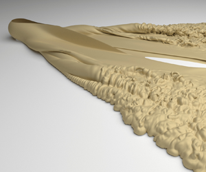
  $a=0.63$. The surface formed by the contour extends behind the source as a wedge of decreasing angle away from the source. Contrary to the axisymmetric release of a dense flow from a stationary source, or the lock-release of a dense flow in a rectangular channel, it is not immediately obvious how the front position relates to the motion of the dense fluid. The source is easily identified by the spherical bulb in figure 2. Complex structures similar in appearance to the lobe-and-cleft instability (Härtel et al. Reference Härtel, Carlsson and Thunblom2000a,Reference Härtel, Meiburg and Neckerb; Necker et al. Reference Necker, Härtel, Kleiser and Meiburg2002, Reference Necker, Härtel, Kleiser and Meiburg2005) are observed at the front of the contour in all directions, and the flow is turbulent close the edge of the wedge. Towards the centreline formed by the path of the source, the flow appears to be laminar. Because the contour does not extend ahead of the source, we find that at
  $a=0.63$, the dense current that forms moves more slowly than the source. As such, we anticipate that the characteristic velocity of the current depends not only on
  $U_b$, but also
  $U_s$, based on the scaling argument introduced in § 2.1. It remains unknown, however, in which direction fluid is advected upon being released from the source, and whether the current propagates in a preferred direction. Figure 3 shows a top view of a slice of the buoyancy
  $b$ at
  $z=0.1$ at various times and for various source speeds
  $a$. For
  $a=0$, the flow is axisymmetric as expected, and propagates in all directions until it reaches the boundaries of the domain, at
  $t\approx 60$. At
  $a=0.3$, the front is still able to advance in all directions around the source, but the source is not at the centre of the current. Instead, the buoyancy is skewed towards the back of the source, i.e. in the direction normal to its motion, and the front of the current forms a more oval shape. The buoyancy is larger at the front, ahead of the source, than behind the source, which is expected as the dense scalar cannot move away from the source as quickly ahead of it. A markedly different behaviour is observed at
  $a=0.63$, for which the dense scalar is only observed behind the source, and no front is observed ahead of the source. As already observed in figure 2, the buoyancy forms a wedge shape behind the source. Visually, the dense scalar buoyancy stops evolving at
  $t\approx 50$, once the wedge has reached the outflow boundary. Note that the simulation at
  $a=0.63$ is conducted in a wider domain (
 $L_y=24$, see table 1), but only the range
  $y=[-10,10]$ is shown in the figure, for presentation. This statistically steady state is observed for all values of
  $a\geq 0.63$. As shown for
  $a=1.26$ in figure 3, however, the flow enters the steady state earlier as
  $a$ increases. The region occupied by the dense scalar is observed to narrow as
  $a$ increases, which is consistent with the decrease in effective buoyancy velocity
  $U_b^{*}$ based on the scaling arguments of § 2.2.

Figure 2. Isosurface of buoyancy  $b=0.1$ at
  $t=63$ for
  $a=0.63$,
  $Re_b=7937$.

Figure 3. Horizontal slice of scalar buoyancy at  $z=0.1$ for various source velocities
  $a$ and at various times
  $t$. At
  $a=0$, the flow is axisymmetric and the front propagates in all directions until it reaches the boundary of the domain. At
  $a=0.378$, while the scalar buoyancy is skewed, the front ahead of the source is still able to move away from the source. At
  $a=0.63$ and
  $a=1.26$, no scalar buoyancy is present ahead of the source. After a certain time, the wedge-shaped region occupied by the scalar buoyancy behind the source enters a steady state. This occurs early (
 $t<30$) in the simulation for
  $a=1.26$, and at
  $t\approx 50$ for
  $a=0.63$.
When the source moves more rapidly than the dense current that it forms, the flow enters a regime whereby perturbations of the front behind the source are unable to travel back upstream towards the source, as the latter moves more rapidly than the dense current. This further suggests that in the reference frame of the moving source, this regime leads to a statistically steady state such that the dimensionality of the system is reduced by removing time dependency. Because disturbances may affect only a limited spatial region behind the source and information cannot travel upstream from the boundary conditions, we refer to this regime as the ‘supercritical regime’. In the statistically steady state, the  $y$ position of the front is a function of the distance
  $x$. The front position is thus non-ambiguously characterized by the furthest position
  $y_f(x,t)$ along the
  $y$-axis where
  $b(x,y_{f},z,t)>b_{t}$ where
  $b_t$ is a threshold value arbitrarily set to
  $b_t = 0.1$. Note that
  $y_f(x,t)$ is only a function of time due to the presence of local disturbances caused by the lobe and cleft instability, and in the following we simply discuss the front position in the supercritical regime as
  $y_f(x)$ where it is understood that the front position is averaged over time once the flow enters the statistically steady state.
Vertical slices of the buoyancy at various positions behind the source are presented in figure 4 for  $a=0.63$ at
  $t=63$. At all positions behind the source a clearly defined region of high buoyancy is present at the ‘head’ of the current in both directions, owing to the symmetry of the problem around the
  $x$-axis. Behind the head, the dense scalar occupies a much thinner region of the domain in the vertical. The height and buoyancy of the head is seen to decrease away from the source. Far from the source, three distinct regions are observed, consisting of the taller, higher buoyancy head, the thinner but turbulent body, and the relatively undisturbed tail. These observations, made at the same time but at different locations behind the source, are reminiscent of the time evolution of a small-length lock-release gravity current in a rectangular channel (Härtel et al. Reference Härtel, Carlsson and Thunblom2000a; Cantero et al. Reference Cantero, Balachandar, García and Bock2008). (This is to be contrasted with finite volume lock-release gravity currents where the lock length is significantly larger than the lock height.) We propose that a simple mechanism in the supercritical regime leads to the similarities between the lock-release problem in a rectangular channel and the moving source problem at high
  $a$. As
  $a$ increases, gradients of density in the direction of motion of the source become smaller, and the gravity current thus propagates predominantly in the
  $y$ direction. Let us consider that transport of dense fluid is constrained to the
  $y$–
$y$– $z$ plane, then the gravity current resulting from the moving source can be seen as an instantaneous release of dense fluid, initiated by the passage of the source through that plane. Under this assumption, the evolution of the current as a function of the distance from the source
  $x$ is equivalently described by the time
  $t$ since the passage of the source through the considered plane, i.e.
  $t' = x/a$. The transition to the supercritical regime is explored systematically as a function of
  $a$ in § 4, and the modelling of the moving source as an instantaneous lock-release gravity current in the high-
 $a$ regime is investigated in § 5.

Figure 4. Vertical slices of scalar buoyancy in the plane normal to the direction of motion of the source, at various distances  $x$ behind the source, for
  $a=0.63$ at
  $t=63$. A clearly defined gravity current head propagates away from the centreline in both directions.
4. Constant flux regime and transition to the supercritical regime
In § 3, we hypothesized that the transition to a supercritical regime occurs when the source moves more rapidly than the gravity current generated by the release of the dense scalar. In order to determine the critical source speed at which this transition occurs, we compute the furthest point  $x_{fr}(t)$ ahead of the source where the buoyancy exceeds a threshold
  $b_t$ as a function of time (figure 5). In the limit case where
  $a=0$, the problem reduces to an axisymmetric constant-flux gravity current. The front position is found to scale as
  $x_{fr}\sim t^{3/4}$. This is in agreement with the box-model approximation of the constant flux axisymmetric gravity current (Huppert Reference Huppert1982; Ungarish Reference Ungarish2020) in the inertial-buoyancy balance. Using the reference quantities introduced in § 2.1, the box-model solution predicts a radial front position
 \begin{equation} r_{bm} =Fr_r t^{{3}/{4}}, \end{equation}
where  $Fr_r$ is the radial Froude number. A least squares fit to the radial front position computed from the numerical simulations yields
  $Fr_r\approx 0.44$ and the fitted box-model solution is superimposed to the radial front position in figure 5.

Figure 5. Front distance from the source ahead of the source  $x_{fr}$ as a function of time for various values of
  $a$. The system goes through a regime change at
  $a=0.63$, above which the front is unable to move past the source. The red dashed line indicates the box-model fit
  $Fr_r t^{{3}/{4}}$ with
  $Fr_r=0.44$ for the axisymmetric case
  $a=0$.
For all values of  $a\leq 0.378$ the dense front is able to move ahead of the source, and therefore moves more quickly than the source itself. For all values
  $a\geq 0.63$, the front position ahead of the source immediately reaches a constant value close to 0, which demonstrates that for
  $a\geq 0.63$, the dense front is always slower than the source itself. Thus, the system enters the supercritical regime in which the aforementioned steady state is obtained for
  $a\geq 0.63$. In the subcritical regime, the gravity current acts as a constant flux release close to the source. However, as the front moves ahead and away from the source, its velocity eventually decreases below
  $a$ when
  $a\neq 0$. Assuming that the box-model solution extends to intermediate values of
  $a$, the front velocity varies as
  $t^{-{1}/{4}}$, such that the time
  $T$ at which the front velocity is equal to the source speed
  $a$ varies as
  $T\sim a^{-4}$, and the corresponding asymptotic position of the front varies as
  $a^{-3}$. In the subcritical regime, a decrease in the source speed leads to a cubic increase in the distance reached by the gravity current ahead of the source and a quartic increase in the time needed to reach this asymptote. It is therefore particularly challenging to investigate the asymptotic behaviour of the subcritical regime numerically, as the domain size needed to observe the asymptotic front position increases as
  $a^{-6}$ and the total simulation time as
  $a^{-4}$ with decreasing
  $a$, leading to a total increase in computational time
  $O(a^{-10})$. We then consider the normal front position
  $y_{f}(x,t)$ (see § 3), plotted in figure 6 for different values of
  $a$. The coloured area represents the standard deviation over time
  $t=50$ to
  $t=63$ from the mean front position averaged over the time interval, and the full lines correspond to this time average. The value of
  $a=0.63$ for the transition to a supercritical regime in which a steady state is obtained in the reference frame of the moving source is further observed with the convergence of the front position. Below
  $a=0.63$, the front position is evolving over the time interval as expected in the subcritical regime. At
  $a\geq 0.63$, variability in the front position is only due to turbulent fluctuations and the front position has statistically converged. In the reference frame of the moving source, the front position becomes time independent for
  $a\geq 0.63$. Thus, the front velocity in the direction normal to the direction of motion of the source, expressed in the stationary reference frame, defined as
 \begin{equation} V_f(x,t) = \frac{\partial y_{f}(x,t)}{\partial t}, \end{equation}
can be expressed, by virtue of the time invariance of  $y_{f}$ in the supercritical regime, as
 \begin{equation} V_f(x)=\frac{\partial x}{\partial t} \frac{\partial y_{f}(x)}{\partial x}= a\frac{\partial y_{f}(x)}{\partial x}.\end{equation}
We thus find that once the flow transitions to the supercritical regime, the dense scalar forms a wedge front behind the source that becomes time independent in the reference frame of the moving source. Note that how far behind the source this steady state is observed is not investigated here, as it depends on the initial transient regime observed in figure 3, and thus on how long the source has been in motion. The front velocity  $V_f$ is computed and further discussed in § 5.

Figure 6. Front position  $y_{f}$ in the reference frame of the moving source as a function of
  $x$ for different source velocities
  $a$. The coloured area corresponds to the standard deviation from the mean front position averaged between
  $t=50$ and
  $t=63$, which corresponds to the full lines.
5. Lock-release model for the supercritical regime
5.1. Available buoyancy
When  $a\gg 1$, in the reference frame of the moving source, (2.3) is dominated by advection by the flow past the source in the
  $x$-direction. The release of the dense scalar, of which the buoyancy is expected to scale with
  $1/a$ in the supercritical regime, thus predominantly results in gradients in the
  $y$-direction, and therefore an increase in momentum in the
  $y$-direction. If we consider a fixed vertical plane normal to the direction of motion of the source, the passage of the source through that plane when
  $a\gg 1$ results in a local increase in buoyancy which then forms a gravity current approximately constrained to that plane since gradients in the spanwise
  $x$-direction become small. (‘Spanwise’ is used to refer to the direction normal to the predominant direction of propagation of the gravity current, consistent with the literature.) With the exception of the shape of the lock, the problem in a fixed
  $y$–
$y$– $z$ plane is analogous to the instantaneous lock-release problem of a gravity current in a rectangular channel. In the limit where the time scale associated with the source motion is much smaller than the time scale associated with buoyancy, i.e.
  ${D}/{U_s}\ll {D}/{U_b}$, the relative mass per unit length released by the passage of the source is simply given by the analytical, non-dimensional expression
 \begin{equation} m_0 = \frac{\rm \pi}{6}\frac{gSD^{3}}{U_s}\cdot\frac{1}{BD^{2}} =\frac{\rm \pi}{6a},\end{equation}
where we recall that  $B={gSD}/{U_b}$ is the reference buoyancy used to non-dimensionalize the equations. Under the same assumptions, the maximum buoyancy generated by the source is found along the centreline of the source trajectory, and is given by
 \begin{equation} b_0 = \frac{gSD}{U_s}\cdot\frac{1}{BD}=\frac{1}{a}.\end{equation}
The relative mass per unit length can be directly compared with the measured mass per unit length computed from the simulations as
 \begin{equation} m_x(x) =\iint_{y,z}b(x,y,z)\,\textrm{d} y\,\textrm{d} z, \end{equation}
and plotted in figure 7(a) for  $t=63$. The mass per unit length is seen to reach a local maximum at some distance behind the source for all values of
  $a$ in the subcritical regime. This supports the previous observation that in the subcritical regime, the dense current spreads in all directions and thus the mass per unit length in the direction of motion of the source varies with distance from the source. In the supercritical regime, however, the buoyancy increases at the source and for a short distance behind the source before reaching a constant value independent of
  $x$. This conservation of mass along the
  $x$-axis in the supercritical regime, on the other hand, demonstrates that the negative buoyancy released by the source spreads over a constant area.

Figure 7. (a) Mass per unit length  $m_x(x) = \iint _{y,z}b(x,y,z)\,\textrm {d} y\,\textrm {d} z$ function of
  $x\in [-1,4]$ for different values of
  $a$ at
  $t=63$. (b) Maximum mass per unit length for different values of
  $a$ at
  $t=63$, plotted against the analytical value in the absence of buoyancy advection or diffusion (see (5.1)).
In figure 7(b), the global maxima of  $m_x$ and the analytical solution
  $m_0$ (see (5.1)) in the limit of no diffusion or advection are plotted as a function of
  $a$, and show excellent agreement for all values of
  $a$ in the supercritical regime, except for
  $a =0.63$, where the analytical formula underestimates the buoyancy, suggesting that other accumulation processes allow the buoyancy to build up at this source velocity.
The excellent agreement between the theoretical mass per unit length in the absence of buoyancy-driven advection or diffusion, expressed in (5.1), and the measured mass per unit length in the simulations when  $a\geq 0.945$ shows that for such high values of
  $a$, the source acts as an instantaneous release of buoyancy in the
  $y$–
$y$– $z$ plane. In § 5.2, we show that this release in buoyancy at high values of
  $a$ drives a flow analogous to small-release gravity currents in the rectilinear configuration.
5.2. Normal front velocity
As shown in § 5.1, the buoyancy generated by the source remains constant within the vertical  $y$–
$y$– $z$ plane, which suggests that in the regime where
  $a>1$, the source does not act as a constant-flux release, but as a constant-volume release constrained to the vertical plane. In the following, we therefore compare the propagation of a rectilinear lock-release (RLR) gravity current with the propagation of the MS gravity currents in the
  $y$-direction. For simplicity, we consider an RLR gravity current with a rectangular lock of height
  $h=1$ and buoyancy
  $b=1$. The length
  $l$ of the lock is set so that the lock has the same area as the MS gravity current in the vertical plane. By symmetry, the propagation of the RLR gravity current is only considered in one half of the vertical plane, such that
  $l=\frac {1}{2}{m_0}/{b_0}={{\rm \pi} }/{12}$. The initial condition of the RLR is sketched in figure 8 alongside a sketch of the vertical slice of buoyancy imparted by the moving source.

Figure 8. Sketch of the RLR gravity current initial condition alongside a sketch of the vertical slice of buoyancy imparted by the moving source in a fixed vertical plane normal to the direction of motion of the source.
Using the same numerical framework, we simulate the RLR gravity current in a channel of height  $1.5$, length
  $10$ and width
  $0.5$. The Reynolds number is set to
  $10\,000$ so as to reproduce the turbulent conditions of the moving source problem. The normal front velocity
  $V_f$ calculated from the moving source simulations can be directly compared with the results of the RLR gravity current simulation by rescaling
  $V_f$ with the buoyancy velocity of the equivalent RLR gravity current, i.e.
  $\sqrt {b_0}=\sqrt {{1}/{a}}$. Considering the moving source problem in the stationary reference frame, the front evolves as a function of time at a given position which relates directly to the distance from the source in the simulations as
  $t'=x/a$. Rescaled with the modified buoyancy velocity, the equivalent spreading time is
  $\tilde t = \sqrt {{1}/{a}}t'=\sqrt {{1}/{a^{3}}}x$.
We now compute the normal front velocity  $V_f$ of the moving source gravity current using (4.3). Here
  $V_f$ is plotted as a function of the equivalent lock-release time
  $\tilde t$ in figure 9. Note that the front position is smoothed over a moving window in order to avoid discontinuities in the spatial derivatives that inevitably arise as a result of the discrete nature of the front position in the simulations. The front velocities for
  $a<0.63$, shown as dashed lines, are plotted for completeness but are outside of the regime of applicability of (4.3) since a steady state is not observed. The front velocity displays a very similar behaviour to small-release gravity currents in rectangular channels (Rottman & Simpson Reference Rottman and Simpson1983; Cantero et al. Reference Cantero, Lee, Balachandar and Garcia2007). For instance, at
  $a=1.26$ and
  $a=1.89$, the front velocity initially increases to a maximum value, then slightly decreases as it enters a phase of constant velocity, and finally starts decreasing after a finite time. At
  $a=2.52$, the numerical domain is too short for the current to enter this decreasing velocity regime and the constant velocity regime is observed until the maximum resolved time. At
  $a=0.945$, the front also reaches a maximum velocity followed by a phase of relatively constant velocity. This phase is, however, followed by a sharp increase in front velocity which precedes an abrupt drop. This unexpected change in front speed is most likely due to the presence of shear-induced, large-scale three-dimensional structures at the front, which do not exist in classical planar currents and are not investigated further here. At
  $a=0.63$, the front velocity quickly increases to a maximum, and promptly enters a phase of velocity decrease. A period of relatively constant velocity is only observed for a short time, for
  $0.6< t'<3.6$. For all values of
  $a> 0.63$, and to a lesser extent for
  $a=0.63$, the rescaled front velocity curves collapse onto a single curve, showing that both the temporal scaling of
  $\tilde t$ and the velocity scaling of
  $\sqrt {{1}/{a}}U_b$ adequately capture the behaviour of the normal front. In addition, the front velocity calculated from the simulation of the RLR gravity current in the rectilinear channel, with lock height
  $1$ and lock length
  ${\rm \pi} /12$, is plotted in figure 9. A time shift of 0.5 non-dimensional times is applied to the RLR in order to align the beginning of the acceleration phase with the moving source simulations. We note that the initial behaviour of the RLR gravity current might differ from that of the moving source as a result of the small lock length to lock height aspect ratio in the RLR simulation, leading to a column-collapse behaviour, which might explain the need for the time shift. The RLR simulation achieves a similar velocity maximum at the end of the acceleration phase and enters a phase of relative constant velocity, followed by a phase of velocity decrease.

Figure 9. Normal front velocity  $V_f$ as a function of the relative time
  $\tilde t$ for various values of
  $a$. The velocity is computed from the time averaged front position and is plotted as a dashed line for
  $a< 0.63$ since the front position has not converged. The vertical dotted lines mark the estimated start and end times of the constant velocity phase for
  $a\geq 0.63$. The black full line represents the front velocity calculated from the RLR DNS with lock height
  $1$ and lock length
  ${\rm \pi} /12$.
The normal front velocity of the MS gravity current is averaged over the time interval of relatively constant front velocity  $\tilde t\in [\tilde t_1,\ \tilde t_2]$. The values of
  $\tilde t_1$ and
  $\tilde t_2$ are estimated as
  $\tilde t_1 \approx 1.64$, 1.79, 1.93, 2.11, 2.28, and
  $\tilde t_2 \approx 3.6$, 8.0, 9.4, 9.7, 10 for
  $a=0.63$, 0.945, 1.26, 1.89, 2.52, respectively. These times are reported in figure 9 as a short vertical dotted line. As for the moving source problem, the beginning and end times of the constant velocity phase are visually estimated and added to figure 9. Close agreement is observed between the RLR gravity current front velocity and the MS gravity current normal front velocity for
  $a>1$. The duration of the constant velocity phase also closely matches that of the simulation at the largest value of
  $a$ tested. The time averaged normal front velocity
  $\bar V_f$ of the MS gravity current is plotted as a function of
  $a$ in figure 10(a), and rescaled with the effective buoyancy
  $\sqrt {{1}/{a}}$ to be directly compared with the time averaged front velocity of the RLR gravity current. In addition, both the MS and RLR gravity current DNS results are compared with the front velocity predicted by the shallow water theory of Rottman & Simpson (Reference Rottman and Simpson1983) for a lock-release gravity current with the same initial lock height to channel height ratio as the RLR gravity current DNS. Great quantitative agreement is found between the normal front velocities of the MS gravity currents for values of
  $a\geq 0.945$ and the RLR gravity current DNS, as observed in figure 9. The observed front velocities of the MS and RLR gravity current DNS are slightly smaller than those predicted by the shallow water model of Rottman & Simpson (Reference Rottman and Simpson1983). This small discrepancy could be a result of the model parameter
  $\beta$, here set to one, or due to the fact that some of the assumptions break down for ratios of initial lock height to channel height larger than
  $\frac {1}{2}$. We note that the agreement between the MS and RLR DNS is good for
  $a\geq 0.945$, but significantly poorer at
  $a=0.63$, which further suggests that while the gravity current enters the supercritical regime at
  $a\approx 0.63$, the released gravity current only behaves as a lock-release current when
  $a\approx 1$ or larger.

Figure 10. (a) Mean front velocity in the constant velocity regime as a function of  $a$ for
  $a\geq 0.63$. The MS gravity current average front velocity is compared with the RLR simulation, and to the solution obtained from the shallow-water equation following Rottman & Simpson (Reference Rottman and Simpson1983) with
  $\beta =1$. (b) Front position relative to initial lock length at the transition time
  $\tilde t_2$ when the current front starts slowing down. The MS simulations and RLR simulation are compared with the experimental observations of Rottman & Simpson (Reference Rottman and Simpson1983).
In addition to the averaged front velocity, we compare the front position of the MS and RLR gravity current fronts at the time when the current starts slowing down from the constant velocity phase. Rottman & Simpson (Reference Rottman and Simpson1983) estimated that the front velocity of gravity currents produced by instantaneous releases in a rectangular channel started decreasing when the front position reached three to 10 lock-lengths depending on the initial lock to channel height ratio, increasing almost linearly with this ratio. For the present lock to channel height ratio of  $\frac {2}{3}$, the findings of Rottman & Simpson (Reference Rottman and Simpson1983) suggest that the current front will start slowing down when it reaches six to nine times the initial lock length. The front position at time
  $\tilde t_2$, is shown as a function of
  $a$ for the MS gravity current simulations in figure 10(b). It is compared with the front position at the transition time
  $\tilde t_2$ computed from the RLR simulation, as well as with the transition distances observed in the experiments of Rottman & Simpson (Reference Rottman and Simpson1983), between
  $6x_0$ and
  $9x_0$ where we recall that
  $x_0 ={{\rm \pi} }/{12}$ is the lock length of the RLR gravity current simulation. The transition distance of the MS gravity current increases with
  $a$ and converges for values of
  $a\geq 1.26$, for which great agreement is found with the RLR gravity current simulation. For
  $a=0.63$, and to a lesser extent
  $a=0.945$, the gravity current travels shorter distances before starting to slow down. Both the RLR simulation and the MS simulations for all values of
  $a$ except
  $a=0.63$ find a longer transition distance than in the experiments of Rottman & Simpson (Reference Rottman and Simpson1983). The relative increase over the upper bound of
  $9x_0$ is approximately
  $30\,\%$ for the RLR simulation. We do not further investigate the cause of this discrepancy.
In summary, the temporal evolution of the MS gravity current front normal to the direction of motion of the source is found to agree well with that of the RLR gravity current with initial buoyancy  $\sqrt {{1}/{a}}$, lock height
  $1$ and lock length
  ${{\rm \pi} }/{12}$. The lock length is chosen such that the mass of the dense fluid contained within the lock is equal to the mass per unit length produced by the spherical moving source in the limit of large values of
  $a$. We also find that while the gravity current enters the supercritical regime when
  $a= 0.63$, and its front velocity in the constant velocity phase is well predicted by the theory of lock-release gravity currents for
  $a= 0.945$, its behaviour is most similar to that of the equivalent lock-release problem when
  $a\geq 1.26$ in our simulations. Above this threshold, the normal front velocity of the MS gravity current in the constant velocity phase is, in dimensional units, approximately equal to
  $Fr\sqrt {{1}/{a}}U_b$ where the Froude number
  $Fr$ can be determined from the equivalent RLR gravity current problem, as shown here.
5.3. Velocity field and transition to lock-release in the supercritical regime
The good quantitative agreement between the front position and velocity of a lock-release gravity current, and the MS gravity current in the constant velocity phase for large values of  $a$, is not observed for
  $a=0.63$ despite the flow having transitioned to the supercritical regime. The horizontal velocity averaged over a height of
  $\frac {1}{2}$ from the bottom,
 \begin{equation} \langle(u,v)\rangle_{{1}/{2}}= 2\int_0^{{1}/{2}} (u,v)\, \textrm{d} z, \end{equation}
is computed and plotted in figure 11 for  $a=0.63$, 0.945 and 2.52 for the
  $y>0$ half of the domain, removing
  $a$ from the
  $x$-component of the velocity so as to visualize the velocity in the stationary reference frame. It is superimposed onto a pseudocolour plot of the magnitude of the horizontal velocity. The contour of buoyancy
  $\langle b \rangle _{{1}/{2}}=0.1$ is shown in red to identify the position of the head of the current. For all values of
  $a$ in the supercritical regime, the velocity magnitude is maximal in the head of the current. The direction of the flow, on the other hand, is markedly different at
  $a=0.63$ when compared with larger values of
  $a$. In the head of the current, the flow is initially predominantly aligned with the
  $y$ direction close to the source, but the velocity vectors quickly align with the direction normal to the front. The realignment of the velocity vectors with the normal to the front is characteristic of axisymmetric dense fronts spreading under their own buoyancy. Thus, despite the front position being statistically invariant in the reference frame of the moving source at
  $a=0.63$, the dense fluid is transported normally to the front in the head of the current, and not along the
  $y$-direction.

Figure 11. Quiver plot of the horizontal velocity expressed in the stationary reference frame, vertically averaged over  $z\in [0, \frac {1}{2}]$,
  $\langle (u,v)\rangle _{{1}/{2}}$, superimposed to a pseudocolour plot of the velocity magnitude
  $\|\langle (u,v)\rangle _{{1}/{2}}\|$. The velocity vectors are plotted at every 50 grid points for readability. The
  $0.1$ contour of buoyancy vertically averaged over
  $z\in [0, \frac {1}{2}]$,
  $\langle b\rangle _{{1}/{2}}$ is added in red to visualize the front of the current. Only the
  $y>0$ half of the domain is shown.
For  $a\geq 0.945$, on the other hand, the velocity vectors in the head of the current are not aligned with the normal to the front, and are instead predominantly aligned with the
  $y$-axis in the entirety of the numerical domain behind the source. In a Lagrangian sense, fluid parcels that make up the head and that contain the dense scalar released by the source are thus transported within the
  $y$–
$y$– $z$ plane throughout the propagation of the current. We finally conclude that despite the transition to the supercritical regime in which the source moves more rapidly than the dense front ahead of the source at
  $a=0.63$, the MS gravity current only undergoes the transition to a unidirectional, instantaneous lock-release current when
  $a\approx 1$.
6. Proof-of-concept laboratory experiments of a collector vehicle as a moving source
Deep-sea mining of polymetallic nodules generates sediment plumes in the wake of the collector vehicles that harvest the nodules by resuspending the top layer of the sediment bed. The particulate suspensions that make up the plumes are denser than the surrounding fluid and are thus expected to drive gravity current dynamics behind the collector. The properties of the particle plume immediately after being released from the collector vehicle are primarily controlled by inertial processes, such as turbulence induced by the discharge jet, or turbulence in the wake of the collector. At some distance behind the collector, however, these inertial processes will have dissipated and the diluted plume will be driven by its own buoyancy. Design and operation choices determine the level of dilution of the plume at this transition from an inertia to buoyancy driven flow. In this section, we present proof-of-concept tow-tank experiments of the gravity current produced by a model deep-sea mining collector discharging a dense fluid in its wake, in order to compare the resulting plume with our idealized spherical source numerical model. We then apply our findings to gain insight into the evolution of plumes produced by a full-scale deep-sea mining collector, in the Appendix (A).
A traverse system, fitted to the top of the 5.5 metre-long tank translates an L-shaped reinforced pipe which connects to the deep-sea mining collector and comes out of the back of the model to produce the discharge. Peristaltic pumps feed dense salty water mixed with green dye through the system, released as an axisymmetric jet in the wake of the model. Pulse dampening was applied to the peristaltic pumps to minimize oscillations of the discharge volume flux. Once the pumps are turned on and the discharge outflow is fully established, the collector model is accelerated to the desired constant velocity. Particle image velocimetry confirmed that the flow field is not influenced by the towing mechanism or by any blockage effect of the channel walls. A wide-angle digital camera was placed below the tank in order to analyse the light intensity coming through the dyed fluid. A light sheet was placed at the top of the tank within the camera's observation window in order to maintain a relatively constant incoming light intensity. This approach, in the absence of a calibration curve that reliably relates dye concentration to light absorption, can only be used to obtain quantitative information about the propagation of the gravity current that results from the dense release. The experimental set-up is sketched in figure 12.

Figure 12. Sketch of the experimental set-up. The traverse system fitted to the tank translates an L-shaped pipe that feeds dense dyed fluid to a circular discharge pipe in the wake of a rigid rectangular box, producing a dense outflow. An upward-facing camera captures the dense plume, lit from the top by a uniform light sheet.
The collector model is  $6.5$ cm wide and
  $5$ cm tall. One experiment was conducted with a neutrally buoyant discharge and four experiments were conducted with a dense discharge at various collector speeds. The discharge flow rate is
  $1.5$ l min
 $^{-1}$ and the relative density of the discharge is
  $1.15$ in all experiments except for the neutrally buoyant experiment where the discharge density is equal to the ambient fluid density. The velocity of the collector is varied between
  $0.13$ and
  $0.27$ m s
 $^{-1}$, such that the volume of fluid displaced by the collector per unit time, i.e.
  $U_sL_cW_c$, is approximately
  $25$ l min
 $^{-1}$ at the lowest velocity. The neutrally buoyant experiment is conducted at a collector speed of 0.21 m s
 $^{-1}$. Since the discharge flow rate is much smaller than the volume displaced by the wake, the change in volume due to the discharge is neglected in the following discussion. The discharge results in a mass flow of excess density
  $\dot m \approx 3.75$ g s
 $^{-1}$. In order to discuss the results of the experiments using the same terminology as established in § 2.1, the source diameter is set to the height of the collector. The ratio of source to buoyancy velocity tested are
  $a=\infty$ (neutrally buoyant), and
  $a=2.47$, 1.52, 1.31 and 1.14 (negatively buoyant). A key limitation of the experiment is the relatively low,
  $O(10^{4})$, collector Reynolds number.
Individual frames from the videos captured by the wide-angle camera placed below the tank were extracted at various times when the collector passed over the observation window. A processing routine was developed to place the frames into the reference frame of the moving collector, which suggested that the discharge evolution behind the collector was statistically steady in the moving reference frame. The light intensity measured in the moving reference frame was averaged over the observation time ( $\approx 4s$) to eliminate fluctuations. The resulting mean light intensity is shown in figure 13 with
  $x=0$ marking the beginning of the wake, immediately behind the collector. The dark, blue central region corresponds to area of higher dye concentration while bright, yellow regions correspond to regions where no dye is present. The relatively sharp gradients of intensity suggest that the discharge evolution is indeed in a statistically steady state in the moving reference frame, and temporal fluctuations are small in scale. Close to the collector, the width of the region in which dye is observed increases slightly with distance from the collector for all values of
  $a$ including the neutrally buoyant base. This small initial expansion can either be due to the volume flux of the carrier fluid at the discharge or to entertainment caused by wake turbulence. Farther away from the collector, the role of collector-to-buoyancy velocity ratio
  $a$ is clearly observed. In the neutrally buoyant experiment, at a distance of approximately one collector width away from the collector, the wake stops expanding and the region where dye is observed does not widen with distance to the collector. As
  $a$ decreases towards unity, the region where dense fluid is observed widens increasingly quickly away from the collector.

Figure 13. Bottom view of the time-averaged light intensity in the reference frame of the moving model collector for different values of  $a$. The white dashed line is the mean front position, calculated by averaging the front position from individual snapshots while removing the
  $20\,\%$ extreme values at each position
  $x$.
$x$.
A mean front position is calculated and shown as a white dashed line in figure 13. First, a Boolean filter is applied to the snapshots in the reference frame of the collector, and the front position  $y_{f}$ is extracted for each position in the
  $x$-direction by finding the closest point above and below
  $y=0$ where the threshold value is exceeded. This is repeated for all snapshots in the observation window and the average front position is calculated at each
  $x$ location. We discard the
  $20\,\%$ extreme values from the averaging to remove imperfections in the snapshots such as dirt and scratches on the tank bottom panel. The lower and upper front positions are averaged and plotted in full lines in figure 14 for the five values of
  $a$. For each value of
  $a$, we compute the front position using the mean front velocity from the RLR numerical simulations. This front position is given as a function of
  $x$ as
  $y=y_0+\bar V_{RLR}\sqrt {{1}/{a^{3}}}x$, where
  $y_0$ is the front position of the collector experiments immediately behind the collector. This is plotted in figure 14 as dashed lines for each value of
  $a$. Reasonable agreement is found between the front position of the experiments and the front position calculated using the predicted constant velocity. Repeatability in the experiments proved challenging due to the large-scale absolute wake instability that occasionally leads to vortex shedding behind the moving collector, and agreement between the experiments and the prediction only qualitatively validates the constant volume lock-release description of the MS gravity current at
  $a>1$. The video of the experiment at
  $a=1.11$ (supplementary movie is available at https://doi.org/10.1017/jfm.2021.654) reveals a high level of complexity of the flow structures behind the collector, including wake-induced vortical structures and discharge-induced pulsations caused by the peristaltic pump despite the use of a pulse dampener. The relatively constant wedge angle, its increase with decreasing value of
  $a$, and the qualitative agreement with the front velocity scaling based on the constant volume lock-release assumption nonetheless suggest that despite the wake and outflow dynamics not being included in the numerical simulations, the moving source modelling approach has merit in practical applications. As a result of the proof-of-concept experiments, the authors are preparing a scaled-up experiment in a larger tow-tank facility. Different release mechanisms for the dense scalar, including a porous sphere, will be used to investigate the role of outflow and wake dynamics on the gravity current spreading, and testing the limits of applicability of the numerical model presented in this work.

Figure 14. Time-averaged relative front position as a function of distance from the model collector for different values of  $a$. The dashed lines correspond to the front position calculated from the average velocity of the RLR gravity current simulation in the constant velocity phase, i.e.
  $y_{f}=y_0+\bar V_{RLR}\sqrt {{1}/{a^{3}}}x$.
7. Conclusion
We conducted DNS of high-Reynolds-number gravity currents released from a moving spherical source of a density-contributing scalar. The canonical set-up attempts to bridge the knowledge gap between the constant-flux, axisymmetric release of a dense plume, and the classic, statistically two-dimensional constant-volume lock-release gravity current in rectilinear channels. The motion of the dense current is controlled by a single non-dimensional number  $a$ defined as the ratio of the source speed
  $U_s$ to a buoyancy velocity
  $U_b$, which only depends on the source diameter and the rate at which it introduces scalar buoyancy into the domain. When
  $a=0$, the flow is axisymmetric around the source. For
  $a\leq 0.63$ in the simulations, the flow spreads in all directions around the source in its reference frame, and the distance that the front is able to reach ahead of the source is anticipated to vary with
  $a^{-3}$, after a transient period that varies with
  $a^{-4}$. Exploring this transient regime is particularly challenging as the computational resources needed to reach the asymptotic front position ahead of the source grow extremely rapidly as
  $a$ decreases. For
  $a\geq 0.63$, however, the system enters a supercritical regime in which the gravity current front propagates more slowly than the source such that no dense scalar can move ahead of the source. The front position quickly reaches a steady state in the reference frame of the moving source, forming a wedge of varying angle that becomes increasingly narrow as
  $a$ increases.
In the supercritical regime, the mass per unit length along the axis that follows the direction of motion of the source was found to be constant behind the source, and to match closely the theoretical value  $m_0$ in the absence of diffusion or advection, defined as
  $m_0={{\rm \pi} }/{6a}$. This showed that in this regime, mass is conserved along each vertical slice normal to the direction of motion of the source. We then showed that the normal front velocity and its temporal evolution for values of
  $a\geq 0.945$ agrees well with that of an RLR gravity current with lock height
  $D$, lock length
  $({{\rm \pi} }/{12})D$ and initial buoyancy equal to the maximum theoretical buoyancy produced by the source, i.e.
  $b_0=({1}/{a})B$, where
  $B$ is the reference buoyancy of the constant-flux axisymmetric gravity current. To demonstrate the similarities between the moving source front in the high
  $a$ regime and the RLR current, we conducted a DNS of the latter for the aforementioned parameters. We find that for sufficiently large values of
  $a$, the rescaled front velocities
  $V_f/\sqrt {{1}/{a}}$ for different values of
  $a$ collapse onto one curve when plotted as a function of the equivalent lock-release time
  $\tilde t =\sqrt {{1}/{a^{3}}}x$. This shows that when
  $a$ is sufficiently large, the front velocity of the current, in the direction normal to the direction of motion of the source, is controlled by the buoyancy released by the source within the vertical plane normal to the direction of motion of the source. Second, the rescaled normal front velocity of the MS gravity current averaged over the phase of relative constant velocity,
  $\bar V_f/\sqrt {{1}/{a}}$, is in great agreement with the time averaged front velocity of the RLR gravity current,
  $\bar V_{RLR}$ when
  $a\geq 0.945$. Third, we found that for
  $a\geq 1.26$, the distance travelled by the MS gravity current front when it exists the constant velocity phase is in great agreement with the distance travelled by the RLR current when it starts slowing down.
We then conducted a series of proof-of-concept laboratory experiments in a tow-tank. A model collector vehicle was connected to a discharge pipe fed with dense dyed fluid, and towed by a traverse system at a constant velocity. Snapshots of the resulting plume were taken from below the tank to extract a time-averaged front position in the reference frame of the moving collector. The neutrally buoyant experiment ( $a=\infty$) showed that while the plume initially expands behind the collector due to wake turbulence and entrainment, it quickly reaches a fixed width. Negatively buoyant experiments, with
  $a$ ranging from
  $a\approx 2.4$ down to
  $a\approx 1.1$, revealed a monotonic increase of the wedge angle formed by the dyed fluid in the wake of the collector as
  $a$ decreased. A time-averaged front position was extracted from the experiments and compared with a front position calculated from the averaged velocity of the RLR gravity current scaled with the moving source buoyancy. Without further assumptions, good agreement was found across values of
  $a$, except for the neutrally buoyant case, which is much more sensitive to wake expansion. We nonetheless consider this agreement to be only qualitative, as larger scale experiments are needed to achieve the appropriate Reynolds number regime characteristic of deep-sea mining activities. Further research is needed to better understand the near-source processes for a variety of discharge mechanisms, how they can influence the gravity current propagation away from the source, and how the resulting gravity current differs or compares with the idealized source introduced in our model.
Supplementary movie
Supplementary movie is available at https://doi.org/10.1017/jfm.2021.654.
Funding
T.P. acknowledges funding through ONR grant N000141812762. E.M. acknowledges support through NSF grants CBET-1803380 and OCE-1924655, as well as by the Army Research Office through grant W911NF-18-1-0379. Computational resources for this work used the Extreme Science and Engineering Discovery Environment (XSEDE), supported by the National Science Foundation, USA, Grant No. TG-CTS150053.
Declaration of interest
The authors report no conflict of interest.
Appendix A. Application to full-scale deep-sea mining collector
While a variety of collector designs are currently being considered, most are expected to operate in a similar range of length and velocity scales. The plume environmental impact analysis of Oebius et al. (Reference Oebius, Becker, Rolinski and Jankowski2001) based on the German mining approach in the Clarion-Clipperton Fracture Zone (known as CCFZ) estimates a sediment discharge of  $\dot m\approx 170\ \mathrm {kg}\ \mathrm {s}^{-1}$ in the wake of a collector spanning 6 m in width, 3 m in height, 7 m in length, and moving at
  $1\ \mathrm {m}\ \mathrm {s}^{-1}$. Aleynik et al. (Reference Aleynik, Inall, Dale and Vink2017) report a sediment discharge of
  $\dot m = 278\ \mathrm {kg}\ \mathrm {s}^{-1}$ for a collector vehicle mining the first 15 cm of the sediment layer and moving at a speed of
  $0.3\ \mathrm {m}\ \mathrm {s}^{-1}$. Similar estimates can be derived from a mass-flow balance analysis, yielding discharge rates of
  $\dot m \sim 300\ \mathrm {kg}\ \mathrm {s}^{-1}$ for a commercial-scale collector of width
  ${\sim}10$ m moving at
  $U_s\sim 0.5\ \mathrm {m}\ \mathrm {s}^{-1}$ and mining the first 15 cm of the sediment layer. It has be argued that only a fraction of the sediment layer being removed by the nodule pick-up mechanism will be resuspended and discharged, typically of the order of 20
  $\%$ (Oebius et al. Reference Oebius, Becker, Rolinski and Jankowski2001; Aleynik et al. Reference Aleynik, Inall, Dale and Vink2017). It, however, remains unclear how this fraction changes depending on operating conditions, nodule lifting mechanism and other design factors. Another challenge is to estimate the dilution of the plume once the wake- and jet-induced turbulence has decayed sufficiently for the negatively buoyant plume to start spreading as a gravity current. Oebius et al. (Reference Oebius, Becker, Rolinski and Jankowski2001) suggest that the plume in the wake of the collector is as wide as the collector and has a height equal to 1.5 collector widths, but this is expected to depend strongly on collector design. Even so, it is known that the flow in the wake of the collector will be highly turbulent (Schröder et al. Reference Schröder, Willert, Schanz, Geisler, Jahn, Gallas and Leclaire2020), as the collector Reynolds number
  $Re = U_sL_c/\nu$ is such that
  $Re>10^{6}$ for all the collector designs considered, to our knowledge. Here,
  $L_c$ is the characteristic size of the collector normal to its direction of motion and can be taken as the largest value between the collector width and the collector height. In the following, the results of our spherical source model are applied to a prototypical collector by assuming that the source diameter is equal to the characteristic collector length, i.e.
  $D=L_c$. The dynamics of the near-collector sediment plume are likely to be greatly influenced by design choices, and the spherical source model is not expected to be an accurate representation of the flow very close to the collector. In the far field, however, in a buoyancy-dominated regime, the details of the discharge mechanism will play a less important role. Design-specific tow-tank experiments can confirm the validity of the model, highlight differences in the near and far-field evolution of the plume, and be used to define source terms that more accurately describe the initial release of the plume than the spherical source.
We consider a commercial-scale collector of characteristic size  $L_c=10$ m moving at
  $U_s=0.5\ \mathrm {m}\ \mathrm {s}^{-1}$ and producing a discharge ranging between
  $\dot m = 60\ \mathrm {kg}\ \mathrm {s}^{-1}$ (
 $20\,\%$ resuspension) and
  $300\ \mathrm {kg}\ \mathrm {s}^{-1}$ (
 $100\,\%$ resuspension). With
  $\rho = 10^{3}\ \mathrm {kg}\ \mathrm {m}^{-3}$,
  $g=9.81\ \mathrm {m}\ \mathrm {s}^{-2}$,
  $D=L_c$ and
  $S={\dot m}/{\rho _0({{\rm \pi} }/{6})D^{3}}$ (see (2.4)), the buoyancy velocity of the plume as a moving source varies from
  $U_b\approx 0.48\ \mathrm {m}\ \mathrm {s}^{-1}$ to
  $U_b\approx 0.83\ \mathrm {m}\ \mathrm {s}^{-1}$, such that the source to buoyancy velocity ratio varies between
  $a\approx 1$ and
  $a\approx 0.6$. The collector-to-buoyancy velocity ratio is thus expected to be between the threshold identified in § 4 for the supercritical regime and the threshold identified in § 5 for the lock-release regime, in most realistic scenarios based on currently available data. From an operational standpoint, the gravity current front generated by the discharge of particles at the back of a commercial mining vehicle is thus expected to move mainly in the direction normal to the motion of the source, but could overtake it for collector designs that effectively maximize the discharge density while minimizing mixing. We note that in the model introduced in § 2.1, the buoyancy source term is not associated with a volume flux. In the case of a deep-sea mining collector, the volume flux of sediment from the seabed should be compensated by a volume flux of water across the bottom boundary. However, for typical deep-sea mining operations, the volume flux of particle is much smaller than the volume of fluid displaced by the collector wake. The ratio of particle volume flux
  $Q_p$ to wake volume flux
  $Q_w$ can be expressed as
  ${Q_p}/{Q_w}={\dot m}/{\rho _p}/{{\rm \pi} D^{2}}/{4U_s}$. With
  $D=10$ m,
  $U_s=0.5$ m s
 $^{-1}$,
  $\dot m=300$ kg s
 $^{-1}$ and
  $\rho _p=2500$ kg m
 $^{-3}$, we find that
  ${Q_p}/{Q_w}\approx 1\,\%$, such that the volume flux of particles can be discarded in the physical model. We also note that while a small fraction of the pumped water will be used to carry the nodules to a surface vessel, collector vehicles have a close to zero net-flux of water, as they discharge most of the water that was pumped to pick up the nodules.


