1 Introduction
The present work belongs to the challenging line of scientific enquiry focusing on the study of quantum turbulence, which is not only interesting in its own right but also contributes to our general understanding of fluid turbulence, as it highlights close similarities as well as distinct differences between flows of quantum and viscous fluids (Skrbek & Sreenivasan Reference Skrbek and Sreenivasan2012; Barenghi, Skrbek & Sreenivasan Reference Barenghi, Skrbek and Sreenivasan2014).
Liquid 4He is, in this context, a unique working medium because it can display both quantum and viscous features. It is characterized by extremely low values of kinematic viscosity, three orders of magnitude smaller than those of air, that is, as low as
 $10^{-8}~\text{m}^{2}~\text{s}^{-1}$
(Donnelly & Barenghi Reference Donnelly and Barenghi1998), and, between approximately 4.2 and 2.2 K, at the saturated vapour pressure, it behaves as a classical viscous fluid, such as water (in this phase, it is called He I). Additionally, at approximately 2.17 K, it undergoes the phase transition to the superfluid state and becomes a quantum fluid, known as He II or superfluid 4He. Its observed properties change dramatically – for example, the liquid heat capacity displays a sharp peak in the vicinity of the transition – and its turbulent flows can often be described by using an effective (temperature-dependent) kinematic viscosity.
$10^{-8}~\text{m}^{2}~\text{s}^{-1}$
(Donnelly & Barenghi Reference Donnelly and Barenghi1998), and, between approximately 4.2 and 2.2 K, at the saturated vapour pressure, it behaves as a classical viscous fluid, such as water (in this phase, it is called He I). Additionally, at approximately 2.17 K, it undergoes the phase transition to the superfluid state and becomes a quantum fluid, known as He II or superfluid 4He. Its observed properties change dramatically – for example, the liquid heat capacity displays a sharp peak in the vicinity of the transition – and its turbulent flows can often be described by using an effective (temperature-dependent) kinematic viscosity.
This behaviour can be understood, at least to a certain extent, if both small and large scales of superfluid 4He flows are considered. A phenomenological (large-scale) model is usually employed, as it can account for various experimental findings. It is known as the two-fluid model and assumes that He II consists of two components. While the normal fluid component is described, within the model, as a gas of thermal excitations carrying the entire entropy content of the liquid, the superfluid component represents a collective state of matter (described by a macroscopic wave function) with zero viscosity. The density ratio of the two components is strongly temperature dependent and, at the superfluid transition temperature, He II consists solely of the normal fluid component. By decreasing the temperature, the relative amount of normal fluid decreases and, below 1 K, it is usually assumed that only the superfluid component remains, that is, He II can be regarded as an inviscid fluid.
In order to describe the small-scale behaviour of superfluid 4He flows quantum mechanics can be used and this leads to the conclusion that the superfluid component may flow potentially. Additionally, the existence of quantized vortices (line-like topological defects within the superfluid component) is postulated to account for the vorticity observed in quantum flows. These vortices are, in He II, singly quantized in units of the quantum of circulation
 $\unicode[STIX]{x1D705}=9.97\times 10^{-8}~\text{m}^{2}~\text{s}^{-1}$
and have been visualized by decorating their ångstrom-sized core with small solid particles that became trapped onto them (Bewley, Lathrop & Sreenivasan Reference Bewley, Lathrop and Sreenivasan2006). Many experiments and numerical simulations have shown that the dynamics of quantized vortices in two-fluid flows of superfluid 4He is very rich, including vortex reconnections and generation of vortex rings. Turbulent flows of He II can therefore be seen, above 1 K, as resulting from the interaction between the two-component fluid and the tangle of quantized vortices.
$\unicode[STIX]{x1D705}=9.97\times 10^{-8}~\text{m}^{2}~\text{s}^{-1}$
and have been visualized by decorating their ångstrom-sized core with small solid particles that became trapped onto them (Bewley, Lathrop & Sreenivasan Reference Bewley, Lathrop and Sreenivasan2006). Many experiments and numerical simulations have shown that the dynamics of quantized vortices in two-fluid flows of superfluid 4He is very rich, including vortex reconnections and generation of vortex rings. Turbulent flows of He II can therefore be seen, above 1 K, as resulting from the interaction between the two-component fluid and the tangle of quantized vortices.
This type of turbulence occurring in superfluid 4He can be experimentally generated in various ways, as discussed, e.g. by Varga, Babuin & Skrbek (Reference Varga, Babuin and Skrbek2015). A common approach, which is relatively easy to implement, is to drive the flow thermally, by using, for example, a heater placed inside the He II bath, resulting in the so-called thermal counterflow. Once the heater is switched on, the normal component moves away from it, while the superfluid component flows in the opposite direction, toward the heater, in order to conserve the null mass flow rate (note that this description is strictly valid only on average, that is, at length scales larger than the mean distance between quantized vortices). Superfluid 4He can also be driven mechanically, by using, for example, an oscillating cylinder (Duda et al. Reference Duda, Švančara, La Mantia, Rotter and Skrbek2015), and the resulting flow type is named coflow (Vinen & Skrbek Reference Vinen and Skrbek2014), because the two components move, again on average, at large enough length scales, in the same direction.
Flows of superfluid 4He display, as mentioned above, distinct differences as well as close similarities compared to those observed in viscous fluids. It has been recently shown that the statistical distributions of the Lagrangian velocities of relatively small particles in steady-state thermal counterflow are characterized, at small enough length scales, by a non-classical broadening of the tails (La Mantia & Skrbek Reference La Mantia and Skrbek2014a ). The outcome, which is independent of the imposed large-scale flow (La Mantia et al. Reference La Mantia, Švančara, Duda and Skrbek2016), can be explained by taking into account the interactions between particles and quantized vortices.
Quantum features seem instead to disappear at large length scales, i.e. at scales larger than the mean distance between quantized vortices, when viscous-like properties are recovered. For example, it has been observed that the vorticity temporal decay follows, at relatively late times, the classical
 $-3/2$
power law, in both coflow (Smith et al.
Reference Smith, Donnelly, Goldenfeld and Vinen1993; Stalp, Skrbek & Donnelly Reference Stalp, Skrbek and Donnelly1999; Zmeev et al.
Reference Zmeev, Walmsley, Golov, McClintock, Fisher and Vinen2015) and counterflow (Skrbek, Gordeev & Soukup Reference Skrbek, Gordeev and Soukup2003; Varga et al.
Reference Varga, Babuin and Skrbek2015; Gao et al.
Reference Gao, Guo, Ľvov, Pomyalov, Skrbek, Varga and Vinen2016). Additionally, the Kolmogorov form of the turbulent energy spectrum has been found in various mechanically driven flows of He II (Maurer & Tabeling Reference Maurer and Tabeling1998; Salort et al.
Reference Salort, Baudet, Castaing, Chabaud, Daviaud, Didelot, Diribarne, Dubrulle, Gagne and Gauthier2010, Reference Salort, Chabaud, Lévêque and Roche2012) and the classical-like shape of the Lagrangian velocity increment distributions has been obtained in steady-state thermal counterflow (La Mantia et al.
Reference La Mantia, Duda, Rotter and Skrbek2013; La Mantia & Skrbek Reference La Mantia and Skrbek2014b
).
$-3/2$
power law, in both coflow (Smith et al.
Reference Smith, Donnelly, Goldenfeld and Vinen1993; Stalp, Skrbek & Donnelly Reference Stalp, Skrbek and Donnelly1999; Zmeev et al.
Reference Zmeev, Walmsley, Golov, McClintock, Fisher and Vinen2015) and counterflow (Skrbek, Gordeev & Soukup Reference Skrbek, Gordeev and Soukup2003; Varga et al.
Reference Varga, Babuin and Skrbek2015; Gao et al.
Reference Gao, Guo, Ľvov, Pomyalov, Skrbek, Varga and Vinen2016). Additionally, the Kolmogorov form of the turbulent energy spectrum has been found in various mechanically driven flows of He II (Maurer & Tabeling Reference Maurer and Tabeling1998; Salort et al.
Reference Salort, Baudet, Castaing, Chabaud, Daviaud, Didelot, Diribarne, Dubrulle, Gagne and Gauthier2010, Reference Salort, Chabaud, Lévêque and Roche2012) and the classical-like shape of the Lagrangian velocity increment distributions has been obtained in steady-state thermal counterflow (La Mantia et al.
Reference La Mantia, Duda, Rotter and Skrbek2013; La Mantia & Skrbek Reference La Mantia and Skrbek2014b
).
It is believed that, at these large scales, the quantized vortex dynamics is smoothed in such a way that the resulting quantum flow behaviour is quite similar to that reported to occur in turbulent flows of viscous fluids, within the inertial range. More precisely, the mutual friction force, arising from the scattering of thermal excitations by quantized vortices, is expected to cause the dynamical locking of the two components of superfluid 4He, at large enough length scales, especially in the case of coflow.
However, for thermal counterflow, it is not straightforward to perform a direct comparison with similar flows of viscous fluids, although, as just noted, some of its large-scale features can be said to be classical-like, that is, thermally driven flows of superfluid 4He seem to lack direct (large-scale) classical analogues – possibly because He II is characterized by an extremely large heat conductivity – and might therefore display quantum features also at large scales (Marakov et al. Reference Marakov, Gao, Guo, Van Sciver, Ihas, McKinsey and Vinen2015; Babuin et al. Reference Babuin, Ľvov, Pomyalov, Skrbek and Varga2016).
The present study focuses on a novel type of quantum coflow, which occurs between two grids oscillating in phase. The flow-induced dynamics of relatively small particles suspended in the liquid is analysed, by using the particle tracking velocimetry technique (Guo et al. Reference Guo, La Mantia, Lathrop and Van Sciver2014), at length scales that are found to be larger than the mean distance between quantized vortices. Additionally, the results obtained in He II (above 1 K) are compared with those due to similar flows of He I, which, as mentioned above, is a viscous fluid.
Oscillating grids have been employed occasionally to study turbulent flows of viscous fluids, as they can generate nearly isotropic turbulence, at least far enough from the flow source, and are characterized by the absence of a mean flow that is instead a distinct feature of steady flows past grids, whose investigation constitutes a well-established field of scientific research, see, for example, Isaza, Salazar & Warhaft (Reference Isaza, Salazar and Warhaft2014) and references therein. Following the seminal work by De Silva & Fernando (Reference De Silva and Fernando1994), most oscillating grid studies in classical fluids focus on the temporal and spatial decay of the flow generated by one oscillating grid, as discussed, e.g. by Honey et al. (Reference Honey, Hershberger, Donnelly and Bolster2014), and, to the best of our knowledge, few investigations have been dedicated to the flows occurring between grids oscillating in phase (Villermaux, Sixou & Gagne Reference Villermaux, Sixou and Gagne1995; Blum et al. Reference Blum, Kunwar, Johnson and Voth2010).
In He II towed grids have been used in order to study the decay of quantum turbulence (Smith et al. Reference Smith, Donnelly, Goldenfeld and Vinen1993; Stalp et al. Reference Stalp, Skrbek and Donnelly1999; Zmeev et al. Reference Zmeev, Walmsley, Golov, McClintock, Fisher and Vinen2015) and steady flows past a grid have also been probed (Salort et al. Reference Salort, Baudet, Castaing, Chabaud, Daviaud, Didelot, Diribarne, Dubrulle, Gagne and Gauthier2010; Varga et al. Reference Varga, Babuin and Skrbek2015), the main outcome being that these flows appear to be classical-like, at large enough scales and above 1 K. The investigation of oscillating grid flows in He II has instead received little attention to date, as solely preliminary results have been published (Honey et al. Reference Honey, Hershberger, Donnelly and Bolster2014) or presented at conferences (Sy et al. Reference Sy, Bourgoin, Diribarne, Gibert, Rousset, Boersma, Breugem, Elsinga, Pecnik, Poelma and Westerweel2015; Švančara & La Mantia Reference Švančara, La Mantia, Šimurda and Bodnár2017).
Duda et al. (Reference Duda, Švančara, La Mantia, Rotter and Skrbek2015) reported that millimetre-sized vortices are shed by a cylinder of rectangular cross-section (10 mm wide and 3 mm high) oscillating in superfluid 4He. The outcome, which strongly supports the view that quantized vortex dynamics has, at large enough scales, a classical-like appearance, motivated the current work. We asked ourselves what happens when these mechanically generated vortical structures merge in He II. Is the classical-like behaviour of coflow still preserved in the absence of large vortices? In order to address the question, we used a pair of oscillating grids and observed the corresponding flow in the region between the grids, where the millimetre-sized vortices shed by the oscillators should have lost their coherence. As shown below, we found that, although large vortical structures are not detected, the statistical behaviour of the generated flows appears to be classical-like, in the range of investigated parameters.
Similarly, in thermal counterflow, the flow-induced dynamics of small particles suspended in He II can be said to be indistinguishable from that expected in turbulent flows of viscous fluids, at length scales larger than the mean distance between quantized vortices and in the absence of large vortical structures (La Mantia et al. Reference La Mantia, Duda, Rotter and Skrbek2013; La Mantia & Skrbek Reference La Mantia and Skrbek2014b ). The main aim of the present series of experiments was then to verify if an analogous behaviour can also be seen in purpose-made mechanically driven flows of He II, in order to address indirectly the open question regarding the large-scale quantum features of thermal counterflow.
The answer we found is that particles probing quantum flows do not appear to be significantly affected by the way in which these flows are driven, at least in the present conditions, and that they behave as if they were tracking classical turbulent flows. Additionally, the work can be viewed as a feasibility study for the new type of quantum flow we devised, calling for more detailed measurements and showing that liquid 4He is indeed a unique working fluid for turbulence research.
2 Methods
We employ the Prague low-temperature flow visualization set-up, described in detail in our previous publications, see La Mantia et al. (Reference La Mantia, Švančara, Duda and Skrbek2016) and references therein. It consists of a low-loss liquid 4He cryostat that, during the experiments, can be kept at temperatures ranging from approximately 1.2 to 4.2 K. The cryostat is initially filled with approximately 100 litres of liquid He I, at atmospheric pressure, and the bath temperature is then decreased by pumping the gas on top of the liquid. When needed, the bath temperature is kept constant by suitably regulating the pumping rate, via a butterfly valve, that is, the present experiments have been performed at constant temperature, at the saturated vapour pressure.
The cryostat 25 mm diameter optical ports are located on its bottom tail, which is our experimental volume, of square cross-section (50 mm sides) and 300 mm high, see La Mantia et al. (Reference La Mantia, Chagovets, Rotter and Skrbek2012) for a schematic view. In the case of the present experiments, two grids are suitably placed inside the tail (see figures 1 and 2) and are linked to a vertical shaft connecting them to a computer-controlled electric motor, placed outside the cryostat, providing in-phase oscillations with 10 mm amplitude and frequencies up to 3 Hz, see Duda et al. (Reference Duda, Švančara, La Mantia, Rotter and Skrbek2015) for a picture of the motor room-temperature arrangement. In order to centre the grids in the middle of our experimental channel, supporting rings are attached to them (see figure 2). Each grid has a square cross-section (35 mm sides) and consists of
 $7\times 7$
equidistant circular holes of 4 mm diameter. We can thus define the mesh size
$7\times 7$
equidistant circular holes of 4 mm diameter. We can thus define the mesh size
 $M=5$
mm as the distance between the centres of two adjacent holes. The grid solidity results therefore equal to 54 %, which is a value larger than that recommended by De Silva & Fernando (Reference De Silva and Fernando1994) for grids oscillating in viscous fluids, i.e. less than 40 % (we do not take into account the supporting rings in the calculation of the solidity).
$M=5$
mm as the distance between the centres of two adjacent holes. The grid solidity results therefore equal to 54 %, which is a value larger than that recommended by De Silva & Fernando (Reference De Silva and Fernando1994) for grids oscillating in viscous fluids, i.e. less than 40 % (we do not take into account the supporting rings in the calculation of the solidity).
Liquid 4He is seeded with small particles made of solid deuterium that are obtained by spraying a small amount of helium and deuterium gas mixture into the bath. Since deuterium solidifies at approximately 20 K, in liquid 4He we obtain solid micrometre-sized particles whose density is slightly larger than that of the liquid. By measuring the terminal velocities of the particles, in the absence of other flow sources, we can estimate, by assuming spherical particles and Stokes regime, the particle diameters; see figure 3 for a relevant statistical distribution and La Mantia et al. (Reference La Mantia, Chagovets, Rotter and Skrbek2012) for further details.

Figure 1. (a) Picture of the bottom part of our experimental set-up, including the camera (right), the cryostat optical tail (middle) and the laser (left). (b) Schematic view of our oscillating grids, inside the cryostat tail; for the sake of clarity, the laser sheet, a few particles and the camera are also displayed; see figure 2 for more details and relevant dimensions.
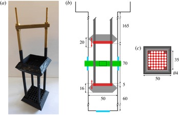
Figure 2. (a) Picture of the flow generator, including its supports. (b) Schematic view of the experimental channel; red rectangles: grids; red arrows: grid stroke; light grey: rings; dark grey: grid supports; green: laser sheet; cyan rectangles: optical ports; small black rectangle between the grids: camera field of view, 13 mm wide and 8 mm high. (c) Schematic view of one grid (dimensions in mm); the square grid (shown in red) consists of
 $7\times 7$
circular holes and is centred in the middle of the experimental channel by using a suitable ring (grey); the four corner holes are occupied by the grid supports.
$7\times 7$
circular holes and is centred in the middle of the experimental channel by using a suitable ring (grey); the four corner holes are occupied by the grid supports.
In order to visualize the suspended particles, we illuminate them by a laser sheet, approximately 1 mm thick and 10 mm high. The corresponding power is approximately 100 mW and the sheet exits the experimental volume from the window opposite to the one through which it goes inside (optical ports are in the middle of the experimental volume sides). A 1 Mpixel CMOS camera, placed at room-temperature perpendicularly to the laser sheet and sharply focused on the illuminated plane, captures the particle positions and collects 400 fps movies, usually made of several hundred frames. The
 $13\times 8~\text{mm}^{2}$
camera field of view is located between the grids, approximately
$13\times 8~\text{mm}^{2}$
camera field of view is located between the grids, approximately
 $6M$
away from each grid, 100 mm from the tail bottom, in the middle of the channel.
$6M$
away from each grid, 100 mm from the tail bottom, in the middle of the channel.

Figure 3. Probability density function (PDF) of the deuterium particle diameter
 $d$
, in
$d$
, in
 $\unicode[STIX]{x03BC}$
m, obtained at 1.95 K (ca. 50 000 velocities; trajectories with at least 20 particle positions). The mean diameter
$\unicode[STIX]{x03BC}$
m, obtained at 1.95 K (ca. 50 000 velocities; trajectories with at least 20 particle positions). The mean diameter
 $d_{p}$
is equal to
$d_{p}$
is equal to
 $7~\unicode[STIX]{x03BC}$
m, while the distribution standard deviation is
$7~\unicode[STIX]{x03BC}$
m, while the distribution standard deviation is
 $3~\unicode[STIX]{x03BC}$
m. Estimation performed following La Mantia et al. (Reference La Mantia, Chagovets, Rotter and Skrbek2012); see the text for further details.
$3~\unicode[STIX]{x03BC}$
m. Estimation performed following La Mantia et al. (Reference La Mantia, Chagovets, Rotter and Skrbek2012); see the text for further details.
The movies are subsequently processed. We detect particle positions and link them into trajectories by using an open-source software (Sbalzarini & Koumoutsakos Reference Sbalzarini and Koumoutsakos2005). We obtain, in each experimental condition, approximately
 $10^{6}$
particle positions and keep for further processing solely tracks with at least five points (on each image we find typically 100 particles; trajectories with up to few hundred points are computed). The time-resolved positions are then linearly differentiated to obtain the corresponding velocities and velocity increments, within the illuminated plane, following a procedure similar to that outlined in La Mantia et al. (Reference La Mantia, Duda, Rotter and Skrbek2013).
$10^{6}$
particle positions and keep for further processing solely tracks with at least five points (on each image we find typically 100 particles; trajectories with up to few hundred points are computed). The time-resolved positions are then linearly differentiated to obtain the corresponding velocities and velocity increments, within the illuminated plane, following a procedure similar to that outlined in La Mantia et al. (Reference La Mantia, Duda, Rotter and Skrbek2013).
Lagrangian velocities are calculated by taking into account three consecutive particle positions. If we consider the horizontal positions
 $x_{1}$
,
$x_{1}$
,
 $x_{2}$
and
$x_{2}$
and
 $x_{3}$
, and the corresponding time intervals,
$x_{3}$
, and the corresponding time intervals,
 $t_{1}$
and
$t_{1}$
and
 $t_{2}$
, we obtain the horizontal velocity at the intermediate position as
$t_{2}$
, we obtain the horizontal velocity at the intermediate position as
 $[(x_{2}-x_{1})/t_{1}+(x_{3}-x_{2})/t_{2}]/2$
(the same scheme is applied to vertical positions; the reference system origin is at the top left corner of the field of view, with the vertical axis pointing downward). In the present case, we do not estimate velocities at the first and last points of the trajectories, which means that the number of velocities is smaller than that of positions. A similar procedure is employed for the velocity increments, which are calculated by taking into account three consecutive velocities, i.e. five consecutive positions (it follows that the number of velocity increments is smaller than that of velocities).
$[(x_{2}-x_{1})/t_{1}+(x_{3}-x_{2})/t_{2}]/2$
(the same scheme is applied to vertical positions; the reference system origin is at the top left corner of the field of view, with the vertical axis pointing downward). In the present case, we do not estimate velocities at the first and last points of the trajectories, which means that the number of velocities is smaller than that of positions. A similar procedure is employed for the velocity increments, which are calculated by taking into account three consecutive velocities, i.e. five consecutive positions (it follows that the number of velocity increments is smaller than that of velocities).
It is apparent that the present grid design is different from that used in other similar water experiments, especially those with pairs of grids oscillating in phase (Villermaux et al. Reference Villermaux, Sixou and Gagne1995; Blum et al. Reference Blum, Kunwar, Johnson and Voth2010). Our grids were made by drilling circular holes into solid plates, not by arrays of equally spaced solid bars (the grid solidity is therefore appreciably larger in our case). Additionally, the chosen grid end conditions, including the supporting rings (see figure 2), are expected to generate vortices of size larger than the grid spacing, which is usually something that should be avoided in classical grid experiments (De Silva & Fernando Reference De Silva and Fernando1994).
However, our main aim was to investigate mechanically driven flows of He II in regions where large vortical structures are absent, not to compare directly our measurements with similar water experiments. We chose therefore for our first series of experiments a grid design that was relatively easy to manufacture, considering our channel geometry, and left for future studies direct comparisons with analogous water measurements. We, nevertheless, also performed experiments in He I, which is a viscous fluid, by using the same grids, in order to assess the classical features of the flows generated by our grids.
Additionally, Honey et al. (Reference Honey, Hershberger, Donnelly and Bolster2014) have reported that (i) the turbulent front due to a classical grid oscillating in water reaches typically, after a relatively short time, a distance from the grid of the order of the channel size (that perpendicular to the oscillations) and that (ii) the latter distance is in He II a few times the channel side, for an oscillating grid having a non-classical design. It follows that, in the present case, as the field of view is located at a distance smaller than the channel side from both grids, we should observe a flow field region where both turbulent fronts are present. We have assumed here that the flow steady state is being studied, as the movies are collected about a minute after the grids are set into motion, and, as discussed below, this indeed appears to be the case.

Figure 4. Typical particle trajectories obtained during one cycle; 13 mm wide and 8 mm high field of view. (a) He I, temperature
 $T=2.53$
K, grid oscillation frequency
$T=2.53$
K, grid oscillation frequency
 $f=1$
Hz; (b) He II,
$f=1$
Hz; (b) He II,
 $T=1.95$
K,
$T=1.95$
K,
 $f=0.5$
Hz; (c)
$f=0.5$
Hz; (c)
 $T=1.95$
K,
$T=1.95$
K,
 $f=1$
Hz; (d)
$f=1$
Hz; (d)
 $T=1.95$
K,
$T=1.95$
K,
 $f=3$
Hz. The oscillation amplitude
$f=3$
Hz. The oscillation amplitude
 $a=10$
mm in all cases.
$a=10$
mm in all cases.
Figure 4 visualizes typical particle trajectories obtained during one cycle, at various temperatures and frequencies. It is apparent that large-scale vortical structures cannot be detected in the region between the oscillating grids, contrary to what has been observed in the proximity of an oscillating cylinder (Duda et al. Reference Duda, Švančara, La Mantia, Rotter and Skrbek2015). If we compare figure 4 with analogous ones obtained in thermal counterflow, see, e.g. La Mantia (Reference La Mantia2016), we notice that, in the latter case, particle motions are mostly parallel to the heat flux direction and that coherent vortical structures are not visible.
We can therefore say that the large-scale appearance of the flows discussed here is different from that seen in the proximity of an oscillating cylinder but, at the same time, it is also not the same as that observed in thermal counterflow. We will show below that this apparent difference does not affect, at large length scales, the shapes of the particle velocity and velocity increment statistical distributions. Similarly, we have already reported that the forms of the particle velocity distribution tails obtained in steady-state thermal counterflow cannot be distinguished from those due to the flows generated by an oscillating cylinder, at scales smaller than the mean distance between quantized vortices (La Mantia et al. Reference La Mantia, Švančara, Duda and Skrbek2016).
The experimental errors of the performed measurements are apparent from the number of significant digits of the quantities reported here. For example, the bath temperature is obtained with a precision of 0.01 K from the measured values of saturated vapour pressure. The error in the particle velocity estimate is equal to approximately
 $0.1~\text{mm}~\text{s}^{-1}$
, due to the accuracy of the used tracking algorithm. Additionally, the tabulated values of some relevant temperature-dependent quantities, such as the fluid density, are employed in this work.
$0.1~\text{mm}~\text{s}^{-1}$
, due to the accuracy of the used tracking algorithm. Additionally, the tabulated values of some relevant temperature-dependent quantities, such as the fluid density, are employed in this work.
3 Length scales
One of the non-classical features of quantum turbulence, resulting from the interactions of flow-probing particles with quantized vortices and leading to the power-law shape of the particle velocity distribution tails, occurs only at small enough length scales, smaller than the mean distance between quantized vortices (La Mantia & Skrbek Reference La Mantia and Skrbek2014a ), regardless of the mechanism of flow generation (La Mantia et al. Reference La Mantia, Švančara, Duda and Skrbek2016).
It is then possible to say that the largest length scale at which one can likely distinguish the actions of individual vortices should be approximately equal to the mean distance
 $\ell$
between quantized vortices, which can be estimated as
$\ell$
between quantized vortices, which can be estimated as
 $1/\sqrt{L}$
, where
$1/\sqrt{L}$
, where
 $L$
denotes the vortex line density (the total length of the vortices in a unitary volume). For steady flows and away from solid boundaries (La Mantia Reference La Mantia2017), as in the present case, we can assume that
$L$
denotes the vortex line density (the total length of the vortices in a unitary volume). For steady flows and away from solid boundaries (La Mantia Reference La Mantia2017), as in the present case, we can assume that
 $L$
is uniform in space and time. The vortex line density can then be calculated from the energy dissipation rate
$L$
is uniform in space and time. The vortex line density can then be calculated from the energy dissipation rate
 $$\begin{eqnarray}\unicode[STIX]{x1D716}=\unicode[STIX]{x1D708}_{eff}(\unicode[STIX]{x1D705}L)^{2},\end{eqnarray}$$
where
 $\unicode[STIX]{x1D708}_{eff}$
is the effective kinematic viscosity associated with turbulent flows of He II; see, e.g. Smith et al. (Reference Smith, Donnelly, Goldenfeld and Vinen1993) for the derivation of equation (3.1) that is mainly motivated by the analogy with the classical turbulence relation between dissipation and vorticity (Tsinober Reference Tsinober2009).
$\unicode[STIX]{x1D708}_{eff}$
is the effective kinematic viscosity associated with turbulent flows of He II; see, e.g. Smith et al. (Reference Smith, Donnelly, Goldenfeld and Vinen1993) for the derivation of equation (3.1) that is mainly motivated by the analogy with the classical turbulence relation between dissipation and vorticity (Tsinober Reference Tsinober2009).
Since, in the range of investigated temperatures,
 $\unicode[STIX]{x1D708}_{eff}$
varies approximately between
$\unicode[STIX]{x1D708}_{eff}$
varies approximately between
 $0.1$
and
$0.1$
and
 $0.3$
times
$0.3$
times
 $\unicode[STIX]{x1D705}$
(Babuin et al.
Reference Babuin, Varga, Skrbek, Lévêque and Roche2014), i.e. is of the order of
$\unicode[STIX]{x1D705}$
(Babuin et al.
Reference Babuin, Varga, Skrbek, Lévêque and Roche2014), i.e. is of the order of
 $10^{-8}~\text{m}^{2}~\text{s}^{-1}$
, we set, for the sake of simplicity,
$10^{-8}~\text{m}^{2}~\text{s}^{-1}$
, we set, for the sake of simplicity,
 $\unicode[STIX]{x1D708}_{eff}=\unicode[STIX]{x1D708}=\unicode[STIX]{x1D707}/\unicode[STIX]{x1D70C}\approx 10^{-8}~\text{m}^{2}~\text{s}^{-1}$
, where the kinematic viscosity
$\unicode[STIX]{x1D708}_{eff}=\unicode[STIX]{x1D708}=\unicode[STIX]{x1D707}/\unicode[STIX]{x1D70C}\approx 10^{-8}~\text{m}^{2}~\text{s}^{-1}$
, where the kinematic viscosity
 $\unicode[STIX]{x1D708}$
of He II is obtained as the ratio between the dynamic viscosity
$\unicode[STIX]{x1D708}$
of He II is obtained as the ratio between the dynamic viscosity
 $\unicode[STIX]{x1D707}$
of its normal component and the total density
$\unicode[STIX]{x1D707}$
of its normal component and the total density
 $\unicode[STIX]{x1D70C}$
of the liquid, both tabulated in Donnelly & Barenghi (Reference Donnelly and Barenghi1998), considering also that
$\unicode[STIX]{x1D70C}$
of the liquid, both tabulated in Donnelly & Barenghi (Reference Donnelly and Barenghi1998), considering also that
 $\unicode[STIX]{x1D708}_{eff}$
is not known with the same accuracy as
$\unicode[STIX]{x1D708}_{eff}$
is not known with the same accuracy as
 $\unicode[STIX]{x1D708}$
.
$\unicode[STIX]{x1D708}$
.
We can compute
 $\unicode[STIX]{x1D716}$
from the imposed grid motion, i.e. from the energy supply rate (Tennekes & Lumley Reference Tennekes and Lumley1972), as
$\unicode[STIX]{x1D716}$
from the imposed grid motion, i.e. from the energy supply rate (Tennekes & Lumley Reference Tennekes and Lumley1972), as
 $$\begin{eqnarray}\unicode[STIX]{x1D716}=\frac{U^{3}}{D}=\frac{(2\unicode[STIX]{x03C0}fa)^{3}}{D},\end{eqnarray}$$
where the grid peak velocity
 $U=2\unicode[STIX]{x03C0}fa$
(
$U=2\unicode[STIX]{x03C0}fa$
(
 $f$
and
$f$
and
 $a$
indicate the grid oscillation frequency and amplitude, respectively) and our channel side
$a$
indicate the grid oscillation frequency and amplitude, respectively) and our channel side
 $D=50$
mm.
$D=50$
mm.
Table 1. Characterization of the experimental runs.
 $T$
denotes the temperature of the 4He bath, in K;
$T$
denotes the temperature of the 4He bath, in K;
 $\unicode[STIX]{x1D70C}_{s}/\unicode[STIX]{x1D70C}$
indicates the ratio between the density
$\unicode[STIX]{x1D70C}_{s}/\unicode[STIX]{x1D70C}$
indicates the ratio between the density
 $\unicode[STIX]{x1D70C}_{s}$
of the superfluid component and that of the liquid, both tabulated in Donnelly & Barenghi (Reference Donnelly and Barenghi1998);
$\unicode[STIX]{x1D70C}_{s}$
of the superfluid component and that of the liquid, both tabulated in Donnelly & Barenghi (Reference Donnelly and Barenghi1998);
 $f$
is the grid oscillation frequency, in Hz; the grid oscillation amplitude
$f$
is the grid oscillation frequency, in Hz; the grid oscillation amplitude
 $a=10$
mm in all cases;
$a=10$
mm in all cases;
 $\unicode[STIX]{x1D716}$
indicates the energy supply rate, in
$\unicode[STIX]{x1D716}$
indicates the energy supply rate, in
 $\text{m}^{2}~\text{s}^{-3}$
, equation (3.2);
$\text{m}^{2}~\text{s}^{-3}$
, equation (3.2);
 $\ell$
is the estimated mean distance between quantized vortices, in
$\ell$
is the estimated mean distance between quantized vortices, in
 $\unicode[STIX]{x03BC}$
m, equation (3.3);
$\unicode[STIX]{x03BC}$
m, equation (3.3);
 $\unicode[STIX]{x1D702}$
and
$\unicode[STIX]{x1D702}$
and
 $\unicode[STIX]{x1D70F}_{\unicode[STIX]{x1D702}}$
denote the Kolmogorov length and time scales, in
$\unicode[STIX]{x1D70F}_{\unicode[STIX]{x1D702}}$
denote the Kolmogorov length and time scales, in
 $\unicode[STIX]{x03BC}\text{m}$
and ms, respectively;
$\unicode[STIX]{x03BC}\text{m}$
and ms, respectively;
 $R$
indicates the ratio between the probed length scale
$R$
indicates the ratio between the probed length scale
 $s_{p}$
, equation (3.4), and the mean particle diameter
$s_{p}$
, equation (3.4), and the mean particle diameter
 $d_{p}=7~\unicode[STIX]{x03BC}\text{m}$
, see figure 3 (the listed values of
$d_{p}=7~\unicode[STIX]{x03BC}\text{m}$
, see figure 3 (the listed values of
 $R$
are the smallest ones, obtained by using the minimum time
$R$
are the smallest ones, obtained by using the minimum time
 $t=2.5~\text{ms}$
between two consecutive frames);
$t=2.5~\text{ms}$
between two consecutive frames);
 $Re$
is the mesh Reynolds number, equation (3.5).
$Re$
is the mesh Reynolds number, equation (3.5).

From equations (3.1) and (3.2) we finally find that the mean distance between quantized vortices
 $$\begin{eqnarray}\ell =\left(\frac{\unicode[STIX]{x1D708}\unicode[STIX]{x1D705}^{2}}{\unicode[STIX]{x1D716}}\right)^{1/4}=\left(\frac{\unicode[STIX]{x1D708}\unicode[STIX]{x1D705}^{2}D}{U^{3}}\right)^{1/4}\end{eqnarray}$$
ranges approximately from 5 to
 $21~\unicode[STIX]{x03BC}$
m; see table 1 for the values of this and other relevant experimental parameters. The smallest viscous scale, i.e. the Kolmogorov dissipative scale, can be calculated as
$21~\unicode[STIX]{x03BC}$
m; see table 1 for the values of this and other relevant experimental parameters. The smallest viscous scale, i.e. the Kolmogorov dissipative scale, can be calculated as
 $\unicode[STIX]{x1D702}=(\unicode[STIX]{x1D708}^{3}/\unicode[STIX]{x1D716})^{1/4}$
, and, for the given experimental conditions, we obtain that
$\unicode[STIX]{x1D702}=(\unicode[STIX]{x1D708}^{3}/\unicode[STIX]{x1D716})^{1/4}$
, and, for the given experimental conditions, we obtain that
 $\unicode[STIX]{x1D702}$
varies between approximately 2 and
$\unicode[STIX]{x1D702}$
varies between approximately 2 and
 $8~\unicode[STIX]{x03BC}$
m.
$8~\unicode[STIX]{x03BC}$
m.
The mean diameter of the particles,
 $d_{p}=7~\unicode[STIX]{x03BC}$
m, see figure 3, is consequently of the same order as
$d_{p}=7~\unicode[STIX]{x03BC}$
m, see figure 3, is consequently of the same order as
 $\ell$
and
$\ell$
and
 $\unicode[STIX]{x1D702}$
, taking into account that the above estimates can solely be regarded as first-order ones. This means that, in the present grid experiments, we can only access large-scale flows (which is confirmed by the results presented below). Additionally, the mean particle displacement
$\unicode[STIX]{x1D702}$
, taking into account that the above estimates can solely be regarded as first-order ones. This means that, in the present grid experiments, we can only access large-scale flows (which is confirmed by the results presented below). Additionally, the mean particle displacement
 $s_{p}$
between two consecutive frames, which is another limiting factor, is even larger. Following Duda et al. (Reference Duda, Švančara, La Mantia, Rotter and Skrbek2015), it is calculated here as
$s_{p}$
between two consecutive frames, which is another limiting factor, is even larger. Following Duda et al. (Reference Duda, Švančara, La Mantia, Rotter and Skrbek2015), it is calculated here as
 $$\begin{eqnarray}s_{p}=Ut=2\unicode[STIX]{x03C0}fat,\end{eqnarray}$$
where
 $t$
indicates the time between consecutive particle positions. As the movies have been taken at 400 f.p.s., the minimum value of
$t$
indicates the time between consecutive particle positions. As the movies have been taken at 400 f.p.s., the minimum value of
 $t$
is 2.5 ms. Note, in passing, that, if we suitably remove positions from the obtained tracks, i.e. if we increase
$t$
is 2.5 ms. Note, in passing, that, if we suitably remove positions from the obtained tracks, i.e. if we increase
 $t$
, larger flow scales can be probed too (see below).
$t$
, larger flow scales can be probed too (see below).
We find that the smallest ratio
 $R$
between the length scale
$R$
between the length scale
 $s_{p}$
, obtained by using
$s_{p}$
, obtained by using
 $t=2.5$
ms in equation (3.4), and the particle size
$t=2.5$
ms in equation (3.4), and the particle size
 $d_{p}$
ranges, in the present conditions, from 12 to 69. As a consequence, we expect that our statistical results are mainly due to the interactions of the particles with many quantized vortices and that we can probe only the particle large-scale flow-induced behaviour. This also follows from the fact that our smallest
$d_{p}$
ranges, in the present conditions, from 12 to 69. As a consequence, we expect that our statistical results are mainly due to the interactions of the particles with many quantized vortices and that we can probe only the particle large-scale flow-induced behaviour. This also follows from the fact that our smallest
 $t$
is of the same order as the Kolmogorov time scale
$t$
is of the same order as the Kolmogorov time scale
 $\unicode[STIX]{x1D70F}_{\unicode[STIX]{x1D702}}=(\unicode[STIX]{x1D708}/\unicode[STIX]{x1D716})^{1/2}$
, see again table 1.
$\unicode[STIX]{x1D70F}_{\unicode[STIX]{x1D702}}=(\unicode[STIX]{x1D708}/\unicode[STIX]{x1D716})^{1/2}$
, see again table 1.
Scales smaller than
 $\ell$
and
$\ell$
and
 $\unicode[STIX]{x1D702}$
could, for example, be investigated by using smaller particles (which is technically challenging) and/or by increasing the camera frame rate, that is, by decreasing the mean particle displacement between consecutive frames. We could also adjust the experiment geometry in such a way that the generated turbulent flows would have larger
$\unicode[STIX]{x1D702}$
could, for example, be investigated by using smaller particles (which is technically challenging) and/or by increasing the camera frame rate, that is, by decreasing the mean particle displacement between consecutive frames. We could also adjust the experiment geometry in such a way that the generated turbulent flows would have larger
 $\ell$
and
$\ell$
and
 $\unicode[STIX]{x1D702}$
, i.e. we could generate oscillatory flows by using small-amplitude, slow oscillations of a large obstacle, e.g. a rectangular cylinder, following Duda et al. (Reference Duda, Švančara, La Mantia, Rotter and Skrbek2015).
$\unicode[STIX]{x1D702}$
, i.e. we could generate oscillatory flows by using small-amplitude, slow oscillations of a large obstacle, e.g. a rectangular cylinder, following Duda et al. (Reference Duda, Švančara, La Mantia, Rotter and Skrbek2015).
If we employ
 $M$
instead of
$M$
instead of
 $D$
in the formula for
$D$
in the formula for
 $\unicode[STIX]{x1D716}$
, equation (3.2), assuming that the vortical structures shed by the grids have sizes of the order of
$\unicode[STIX]{x1D716}$
, equation (3.2), assuming that the vortical structures shed by the grids have sizes of the order of
 $M$
, we find values of
$M$
, we find values of
 $\ell$
and
$\ell$
and
 $\unicode[STIX]{x1D702}$
approximately two times smaller, while
$\unicode[STIX]{x1D702}$
approximately two times smaller, while
 $\unicode[STIX]{x1D70F}_{\unicode[STIX]{x1D702}}$
is about three times smaller, that is, our conclusion that the particles probe large-scale flow properties is still valid. Note, however, that, due to the non-classical design of our grid set-up, we expect that the average size of the vortical structures shed by the grids is larger than
$\unicode[STIX]{x1D70F}_{\unicode[STIX]{x1D702}}$
is about three times smaller, that is, our conclusion that the particles probe large-scale flow properties is still valid. Note, however, that, due to the non-classical design of our grid set-up, we expect that the average size of the vortical structures shed by the grids is larger than
 $M$
.
$M$
.
In order to characterize our measurements and perform relevant comparisons with similar water experiments, especially those with pairs of grids oscillating in phase (Villermaux et al. Reference Villermaux, Sixou and Gagne1995; Blum et al. Reference Blum, Kunwar, Johnson and Voth2010), we can now introduce the mesh Reynolds number
 $$\begin{eqnarray}Re=\frac{2\unicode[STIX]{x03C0}faM\unicode[STIX]{x1D70C}}{\unicode[STIX]{x1D707}}=\frac{UM}{\unicode[STIX]{x1D708}},\end{eqnarray}$$
where
 $M=5$
mm denotes the mesh size.
$M=5$
mm denotes the mesh size.
If we compute
 $Re$
by using the previous equation for the experiments performed by Villermaux et al. (Reference Villermaux, Sixou and Gagne1995), we find that it ranges between approximately 56 500 and 188 600, i.e. it is, in most cases, noticeably larger than our values, listed in table 1. The corresponding energy supply rates, obtained from equation (3.2), are even larger, e.g. more than 2000 times larger when we compare their fastest oscillations with our experiments in He I. Other comparisons with the work by Villermaux et al. (Reference Villermaux, Sixou and Gagne1995) are at present not possible, because we do not have access to Eulerian flow properties and we did not actually observe intense vortical structures, leaving aside the different grid designs. In other words, our focus here is not on rare events, as in Villermaux et al. (Reference Villermaux, Sixou and Gagne1995), but on the Lagrangian large-scale features of the new type of quantum flow we devised.
$Re$
by using the previous equation for the experiments performed by Villermaux et al. (Reference Villermaux, Sixou and Gagne1995), we find that it ranges between approximately 56 500 and 188 600, i.e. it is, in most cases, noticeably larger than our values, listed in table 1. The corresponding energy supply rates, obtained from equation (3.2), are even larger, e.g. more than 2000 times larger when we compare their fastest oscillations with our experiments in He I. Other comparisons with the work by Villermaux et al. (Reference Villermaux, Sixou and Gagne1995) are at present not possible, because we do not have access to Eulerian flow properties and we did not actually observe intense vortical structures, leaving aside the different grid designs. In other words, our focus here is not on rare events, as in Villermaux et al. (Reference Villermaux, Sixou and Gagne1995), but on the Lagrangian large-scale features of the new type of quantum flow we devised.
Slightly smaller maximum values of
 $Re$
and
$Re$
and
 $\unicode[STIX]{x1D716}$
are obtained for the experiments performed by Blum et al. (Reference Blum, Kunwar, Johnson and Voth2010), if the central flow region, between the oscillating grids, is considered, that is, they are still appreciably larger than ours. Additionally, the work by Blum et al. (Reference Blum, Kunwar, Johnson and Voth2010) focuses on conditional structure functions, both Eulerian and Lagrangian, which we cannot presently estimate with the same accuracy, mainly due to the significantly smaller size of our data sets.
$\unicode[STIX]{x1D716}$
are obtained for the experiments performed by Blum et al. (Reference Blum, Kunwar, Johnson and Voth2010), if the central flow region, between the oscillating grids, is considered, that is, they are still appreciably larger than ours. Additionally, the work by Blum et al. (Reference Blum, Kunwar, Johnson and Voth2010) focuses on conditional structure functions, both Eulerian and Lagrangian, which we cannot presently estimate with the same accuracy, mainly due to the significantly smaller size of our data sets.
In summary, direct comparisons between our measurements and those just mentioned are currently difficult to carry out because we solely have information on particle dynamics in the central flow region and cannot characterize quantitatively the flow from the Eulerian point of view. In the following we will therefore compare our Lagrangian results with experiments on other types of turbulent flows, focusing on more general features, which are not only relevant to classical oscillating grid experiments.
4 Velocity distributions
In figure 5 the probability density function of the dimensionless instantaneous particle velocity
 $(u-u_{m})/u_{sd}$
in the horizontal direction (that perpendicular to the imposed grid oscillation) is plotted, at the smallest accessible length scale ratio
$(u-u_{m})/u_{sd}$
in the horizontal direction (that perpendicular to the imposed grid oscillation) is plotted, at the smallest accessible length scale ratio
 $R$
, for all data sets, see table 1 for the experimental run characterization;
$R$
, for all data sets, see table 1 for the experimental run characterization;
 $u_{m}$
and
$u_{m}$
and
 $u_{sd}$
denote the mean and the standard deviation of the dimensional velocity
$u_{sd}$
denote the mean and the standard deviation of the dimensional velocity
 $u$
, respectively, see table 2 for relevant values.
$u$
, respectively, see table 2 for relevant values.
Figure 5. PDF of the normalized particle velocity
 $(u-u_{m})/u_{sd}$
in the horizontal direction, at the smallest
$(u-u_{m})/u_{sd}$
in the horizontal direction, at the smallest
 $R$
;
$R$
;
 $u_{m}$
and
$u_{m}$
and
 $u_{sd}$
indicate the mean value and the standard deviation of the dimensional velocity
$u_{sd}$
indicate the mean value and the standard deviation of the dimensional velocity
 $u$
, respectively (between
$u$
, respectively (between
 $0.5\times 10^{6}$
and
$0.5\times 10^{6}$
and
 $1.7\times 10^{6}$
velocities). Trajectories with at least five particle positions; the area below the data curves is normalized to unity. For the data set characterization, see tables 1 and 2 (the corresponding symbols are indicated in the panel legends). Magenta line: standard Gaussian distribution. Note that the data set A, obtained in He I, is plotted in all panels for the sake of comparison.
$1.7\times 10^{6}$
velocities). Trajectories with at least five particle positions; the area below the data curves is normalized to unity. For the data set characterization, see tables 1 and 2 (the corresponding symbols are indicated in the panel legends). Magenta line: standard Gaussian distribution. Note that the data set A, obtained in He I, is plotted in all panels for the sake of comparison.
It is apparent that the distribution shapes are nearly Gaussian, similarly to what is usually observed in turbulent flows of viscous fluids, within the inertial range. For example, Eulerian velocity distributions have been found, both numerically (Vincent & Meneguzzi Reference Vincent and Meneguzzi1991) and experimentally (Noullez et al. Reference Noullez, Wallace, Lempert, Miles and Frisch1997), to be very close to the Gaussian form, and the same have been reported to occur in the Lagrangian case (Mordant, Lévêque & Pinton Reference Mordant, Lévêque and Pinton2004a ).
Paoletti et al. (Reference Paoletti, Fisher, Sreenivasan and Lathrop2008) showed instead that particle velocity distributions are characterized in decaying thermal counterflow by power-law tails, which can be explained by taking into account the interactions between particles and quantized vortices. The numerical simulations performed by Baggaley & Barenghi (Reference Baggaley and Barenghi2011) at very low temperatures, in the absence of normal fluid flow, confirmed the experimental result and suggested that, at scales larger than the mean distance
 $\ell$
between quantized vortices, a classical-like shape of the distributions should be obtained.
$\ell$
between quantized vortices, a classical-like shape of the distributions should be obtained.
The numerical outcome was experimentally proven by La Mantia & Skrbek (Reference La Mantia and Skrbek2014a
), who reported that, in steady-state thermal counterflow, the power-law tails of the velocity distributions gradually disappear, as the length scale probed by the particles increases, until, at scales larger than
 $\ell$
, the velocity distribution form becomes nearly Gaussian. More recently, this scale dependence has been also observed in the proximity of an oscillating cylinder (La Mantia et al.
Reference La Mantia, Švančara, Duda and Skrbek2016), that is, the velocity distribution shapes appear not to depend on the quantum flow driving mechanism but solely on the probed length scale.
$\ell$
, the velocity distribution form becomes nearly Gaussian. More recently, this scale dependence has been also observed in the proximity of an oscillating cylinder (La Mantia et al.
Reference La Mantia, Švančara, Duda and Skrbek2016), that is, the velocity distribution shapes appear not to depend on the quantum flow driving mechanism but solely on the probed length scale.
The distribution forms displayed in figure 5 are therefore consistent with the assumption made above that we are presently probing scales larger than the mean distance between quantized vortices. Additionally, it can be noted that, as
 $R$
decreases, the distributions become wider, that is, the deviation from the Gaussian shape we observe for the velocity distributions can also be related to the gradual disappearance of the distribution power-law tails as the probed length scale is increased.
$R$
decreases, the distributions become wider, that is, the deviation from the Gaussian shape we observe for the velocity distributions can also be related to the gradual disappearance of the distribution power-law tails as the probed length scale is increased.
If we remove particle positions from the tracks obtained at the smallest time between frames, we can compute the statistical distributions at even larger
 $R$
and we find that their shape is still nearly Gaussian. Figure 6 shows such distributions for the data sets obtained at 1 Hz, at the largest accessible
$R$
and we find that their shape is still nearly Gaussian. Figure 6 shows such distributions for the data sets obtained at 1 Hz, at the largest accessible
 $R$
(the outcome is similar in other cases). Note, in passing, that the ratio between the mesh size and the particle diameter is 714, that is, the length scales probed in figure 6 are larger than (or of the same order of)
$R$
(the outcome is similar in other cases). Note, in passing, that the ratio between the mesh size and the particle diameter is 714, that is, the length scales probed in figure 6 are larger than (or of the same order of)
 $M$
.
$M$
.
Table 2. Mean values (subscript
 $m$
) and standard deviations (subscript
$m$
) and standard deviations (subscript
 $sd$
) of the particle velocities obtained at the smallest
$sd$
) of the particle velocities obtained at the smallest
 $R$
, in the horizontal (indicated by
$R$
, in the horizontal (indicated by
 $u$
) and vertical (denoted by
$u$
) and vertical (denoted by
 $v$
) directions, in
$v$
) directions, in
 $\text{mm}~\text{s}^{-1}$
. The latter is parallel to the grid oscillating motion, while the former is perpendicular to it (the reference system origin is at the top left corner of the field of view, with the vertical axis pointing downward). See table 1 for the experimental run characterization.
$\text{mm}~\text{s}^{-1}$
. The latter is parallel to the grid oscillating motion, while the former is perpendicular to it (the reference system origin is at the top left corner of the field of view, with the vertical axis pointing downward). See table 1 for the experimental run characterization.

The distributions appear, however, to be tilted, mostly toward negative values, and this likely indicates that our field of view in not exactly in the middle of the channel, as this velocity asymmetry is observed for all data sets (the reference system origin is at the top left corner of the field of view, with the vertical axis pointing downward). Additionally, in the case of He I, the distribution tilt is more apparent and the deviation from the Gaussian shape more pronounced than for the data obtained in superfluid 4He.

Figure 6. PDF of
 $(u-u_{m})/u_{sd}$
, at the largest
$(u-u_{m})/u_{sd}$
, at the largest
 $R$
, for the 1 Hz data sets (at least 90 000 velocities). Symbols as in figure 5 (note, however, that the length scale ratio is not the same).
$R$
, for the 1 Hz data sets (at least 90 000 velocities). Symbols as in figure 5 (note, however, that the length scale ratio is not the same).
The finding could be related to the fact that heat dissipates in He II at a much faster rate than in He I. The liquid thermal diffusivity is indeed approximately
 $10^{9}$
times smaller in He I, at 2.53 K, compared to that obtained in He II, at 1.95 K, with a heat flux of
$10^{9}$
times smaller in He I, at 2.53 K, compared to that obtained in He II, at 1.95 K, with a heat flux of
 $1~\text{kW}~\text{m}^{-2}$
; the values of relevant quantities tabulated in Van Sciver (Reference Van Sciver2012), such as the fluid heat capacity, have been used for this estimate. Note that the spatial temperature gradient in He II can be said to be proportional to the cube of the heat flux, while in classical fluids their relation is linear, and that the thermal conductivity of superfluid 4He has a peak at approximately 1.9 K, at the saturated vapour pressure.
$1~\text{kW}~\text{m}^{-2}$
; the values of relevant quantities tabulated in Van Sciver (Reference Van Sciver2012), such as the fluid heat capacity, have been used for this estimate. Note that the spatial temperature gradient in He II can be said to be proportional to the cube of the heat flux, while in classical fluids their relation is linear, and that the thermal conductivity of superfluid 4He has a peak at approximately 1.9 K, at the saturated vapour pressure.
The heat input to the experimental volume due to the oscillating grids can be estimated to be less than
 $300~\text{W}~\text{m}^{-2}$
, while that due to the laser sheet can be said to be lower than
$300~\text{W}~\text{m}^{-2}$
, while that due to the laser sheet can be said to be lower than
 $100~\text{W}~\text{m}^{-2}$
. It follows that in He I this heat results in parasitic flows that decay at a much slower rate than in He II, the corresponding diffusions times being approximately hours and
$100~\text{W}~\text{m}^{-2}$
. It follows that in He I this heat results in parasitic flows that decay at a much slower rate than in He II, the corresponding diffusions times being approximately hours and
 $\unicode[STIX]{x03BC}$
s, respectively. As movies have been collected about a minute after the grids are set into motion in all cases, we can conclude that our He II data should be less affected by the parasitic heat input compared to those obtained in He I, and this is indeed what could explain the more pronounced departure from the Gaussian form observed in figure 5 for the viscous case.
$\unicode[STIX]{x03BC}$
s, respectively. As movies have been collected about a minute after the grids are set into motion in all cases, we can conclude that our He II data should be less affected by the parasitic heat input compared to those obtained in He I, and this is indeed what could explain the more pronounced departure from the Gaussian form observed in figure 5 for the viscous case.
Normalized vertical velocity distributions are not shown here because they do not display features different from those seen from the horizontal ones. We may, however, note that the particle settling velocity is, in the present conditions, approximately
 $1~\text{mm}~\text{s}^{-1}$
, which is a value appreciably smaller than the grid peak velocity (equal, for example, to
$1~\text{mm}~\text{s}^{-1}$
, which is a value appreciably smaller than the grid peak velocity (equal, for example, to
 $31~\text{mm}~\text{s}^{-1}$
at the lowest frequency) and a few times smaller than the obtained particle velocity standard deviations, see table 2. Additionally, the last line of table 2 shows that the probed flows cannot be considered isotropic ones, similarly to what has been observed in thermal counterflow, see, e.g. La Mantia (Reference La Mantia2016), and in the case of turbulent flows between two grids oscillating in water (Blum et al.
Reference Blum, Kunwar, Johnson and Voth2010).
$31~\text{mm}~\text{s}^{-1}$
at the lowest frequency) and a few times smaller than the obtained particle velocity standard deviations, see table 2. Additionally, the last line of table 2 shows that the probed flows cannot be considered isotropic ones, similarly to what has been observed in thermal counterflow, see, e.g. La Mantia (Reference La Mantia2016), and in the case of turbulent flows between two grids oscillating in water (Blum et al.
Reference Blum, Kunwar, Johnson and Voth2010).
Another striking feature of figure 5 is that, in the range of investigated parameters, the shape of the velocity distributions does not seem to depend appreciably on temperature, that is, on the ratio
 $\unicode[STIX]{x1D70C}_{s}/\unicode[STIX]{x1D70C}$
between the density
$\unicode[STIX]{x1D70C}_{s}/\unicode[STIX]{x1D70C}$
between the density
 $\unicode[STIX]{x1D70C}_{s}$
of the superfluid component and that of the liquid, see table 1, possibly because
$\unicode[STIX]{x1D70C}_{s}$
of the superfluid component and that of the liquid, see table 1, possibly because
 $\unicode[STIX]{x1D708}_{eff}$
does not vary much with temperature above 1 K (Babuin et al.
Reference Babuin, Varga, Skrbek, Lévêque and Roche2014). It follows that the latter ratio might not be a relevant parameter in the current case or that, at least, it might have less influence on the distribution form than the length scale ratio
$\unicode[STIX]{x1D708}_{eff}$
does not vary much with temperature above 1 K (Babuin et al.
Reference Babuin, Varga, Skrbek, Lévêque and Roche2014). It follows that the latter ratio might not be a relevant parameter in the current case or that, at least, it might have less influence on the distribution form than the length scale ratio
 $R$
, as it is also apparent from the computational results of Baggaley & Barenghi (Reference Baggaley and Barenghi2011). Similarly, Krstulovic (Reference Krstulovic2016) performed recently numerical simulations on superfluid flow past a grid at very low temperatures, in the absence of normal fluid flow, and found that the computed (Eulerian) velocity increment distributions have classical-like, scale-dependent shapes.
$R$
, as it is also apparent from the computational results of Baggaley & Barenghi (Reference Baggaley and Barenghi2011). Similarly, Krstulovic (Reference Krstulovic2016) performed recently numerical simulations on superfluid flow past a grid at very low temperatures, in the absence of normal fluid flow, and found that the computed (Eulerian) velocity increment distributions have classical-like, scale-dependent shapes.
We conclude this section by saying that the observed nearly Gaussian form of the velocity distributions can also be seen as a consequence of the central limit theorem, that is, a more convincing proof that the probed flows are indeed turbulent ones is given in the next section, on (Lagrangian) velocity increment distributions.
5 Velocity increment distributions
Figure 7 displays the probability density function of the dimensionless instantaneous particle velocity increment
 $(du-du_{m})/du_{sd}$
in the horizontal direction, at the smallest accessible length scale ratio
$(du-du_{m})/du_{sd}$
in the horizontal direction, at the smallest accessible length scale ratio
 $R$
, for all data sets, see table 1 for the experimental run characterization;
$R$
, for all data sets, see table 1 for the experimental run characterization;
 $du_{m}$
and
$du_{m}$
and
 $du_{sd}$
denote the mean and the standard deviation of the dimensional velocity increment
$du_{sd}$
denote the mean and the standard deviation of the dimensional velocity increment
 $du$
, respectively, see table 3 for relevant values.
$du$
, respectively, see table 3 for relevant values.
We can notice that the distributions have wide tails, up to approximately 25 times
 $du_{sd}$
, and are therefore much wider than the Gaussian one, shown, for example, in figure 5. Additionally, all distributions overlap, i.e. the particle velocity increments seem to behave similarly in He I and He II, at different temperatures and oscillation frequencies. We might therefore argue that the observed large-scale flows of He II are indeed viscous-like, considering also that the corresponding velocity distribution forms do not seem to depend appreciably on temperature, as shown above.
$du_{sd}$
, and are therefore much wider than the Gaussian one, shown, for example, in figure 5. Additionally, all distributions overlap, i.e. the particle velocity increments seem to behave similarly in He I and He II, at different temperatures and oscillation frequencies. We might therefore argue that the observed large-scale flows of He II are indeed viscous-like, considering also that the corresponding velocity distribution forms do not seem to depend appreciably on temperature, as shown above.

Figure 7. PDF of the normalized particle velocity increment
 $(du-du_{m})/du_{sd}$
in the horizontal direction, at the smallest
$(du-du_{m})/du_{sd}$
in the horizontal direction, at the smallest
 $R$
;
$R$
;
 $du_{m}$
and
$du_{m}$
and
 $du_{sd}$
indicate the mean value and the standard deviation of the dimensional velocity increment
$du_{sd}$
indicate the mean value and the standard deviation of the dimensional velocity increment
 $du$
, respectively (between
$du$
, respectively (between
 $0.4\times 10^{6}$
and
$0.4\times 10^{6}$
and
 $1.5\times 10^{6}$
velocity increments). Symbols as in figure 5, see tables 1 and 3 for further details. Magenta line: tracer fit obtained in turbulent flows of viscous fluids, equation (5.1) with
$1.5\times 10^{6}$
velocity increments). Symbols as in figure 5, see tables 1 and 3 for further details. Magenta line: tracer fit obtained in turbulent flows of viscous fluids, equation (5.1) with
 $s=1$
(Mordant, Crawford & Bodenschatz Reference Mordant, Crawford and Bodenschatz2004b
); orange line: inertial particle fit obtained in turbulent flows of viscous fluids, equation (5.1) with
$s=1$
(Mordant, Crawford & Bodenschatz Reference Mordant, Crawford and Bodenschatz2004b
); orange line: inertial particle fit obtained in turbulent flows of viscous fluids, equation (5.1) with
 $s=0.62$
(Qureshi et al.
Reference Qureshi, Bourgoin, Baudet, Cartellier and Gagne2007, Reference Qureshi, Arrieta, Baudet, Cartellier, Gagne and Bourgoin2008).
$s=0.62$
(Qureshi et al.
Reference Qureshi, Bourgoin, Baudet, Cartellier and Gagne2007, Reference Qureshi, Arrieta, Baudet, Cartellier, Gagne and Bourgoin2008).
The argument is reinforced by the fact that the distribution shape is consistent with that obtained in turbulent flows of viscous fluids, shown as the magenta line in figure 7 and computed as
 $$\begin{eqnarray}\text{PDF}=\frac{\exp (3s^{2}/2)}{4\sqrt{3}}\left[1-\text{erf}\left(\frac{\text{ln}|b/\sqrt{3}|+2s^{2}}{\sqrt{2}s}\right)\right],\end{eqnarray}$$
where
 $s=1$
and
$s=1$
and
 $b=(du-du_{m})/du_{sd}$
. This functional form has been reported by Mordant et al. (Reference Mordant, Crawford and Bodenschatz2004b
) in their experimental study on the dynamics of fluid particles in classical turbulence, while the shape of the distributions due to inertial particles is characterized by
$b=(du-du_{m})/du_{sd}$
. This functional form has been reported by Mordant et al. (Reference Mordant, Crawford and Bodenschatz2004b
) in their experimental study on the dynamics of fluid particles in classical turbulence, while the shape of the distributions due to inertial particles is characterized by
 $s=0.62$
(Qureshi et al.
Reference Qureshi, Bourgoin, Baudet, Cartellier and Gagne2007, Reference Qureshi, Arrieta, Baudet, Cartellier, Gagne and Bourgoin2008). It follows that, at the smallest scale we can probe, approximately one order of magnitude larger than
$s=0.62$
(Qureshi et al.
Reference Qureshi, Bourgoin, Baudet, Cartellier and Gagne2007, Reference Qureshi, Arrieta, Baudet, Cartellier, Gagne and Bourgoin2008). It follows that, at the smallest scale we can probe, approximately one order of magnitude larger than
 $\ell$
or
$\ell$
or
 $\unicode[STIX]{x1D702}$
, our particles can be regarded in most cases as fluid ones, although inertial effects cannot be neglected (solid deuterium is slightly denser than liquid 4He). Nevertheless, the main result here is that these particles, in the range of investigated parameters, behave as if they were tracking turbulent flows of viscous fluids.
$\unicode[STIX]{x1D702}$
, our particles can be regarded in most cases as fluid ones, although inertial effects cannot be neglected (solid deuterium is slightly denser than liquid 4He). Nevertheless, the main result here is that these particles, in the range of investigated parameters, behave as if they were tracking turbulent flows of viscous fluids.
Table 3. Standard deviations (subscript
 $sd$
) of the particle velocity increments obtained at the smallest
$sd$
) of the particle velocity increments obtained at the smallest
 $R$
, in the horizontal (indicated by
$R$
, in the horizontal (indicated by
 $du$
) and vertical (denoted by
$du$
) and vertical (denoted by
 $dv$
) directions, in
$dv$
) directions, in
 $\text{mm}~\text{s}^{-2}$
. The corresponding mean values are of the order of
$\text{mm}~\text{s}^{-2}$
. The corresponding mean values are of the order of
 $1~\text{mm}~\text{s}^{-2}$
. See table 1 for the experimental run characterization.
$1~\text{mm}~\text{s}^{-2}$
. See table 1 for the experimental run characterization.
Figure 8. PDF of
 $(du-du_{m})/du_{sd}$
, at
$(du-du_{m})/du_{sd}$
, at
 $R=23$
, for the 1 Hz data sets. Symbols as in figure 7. Magenta line: tracer fit obtained in turbulent flows of viscous fluids, equation (5.1) with
$R=23$
, for the 1 Hz data sets. Symbols as in figure 7. Magenta line: tracer fit obtained in turbulent flows of viscous fluids, equation (5.1) with
 $s=1$
(Mordant et al.
Reference Mordant, Crawford and Bodenschatz2004b
); orange line: power-law fit
$s=1$
(Mordant et al.
Reference Mordant, Crawford and Bodenschatz2004b
); orange line: power-law fit
 $\text{PDF}=0.15|b|^{-7/2}$
, where
$\text{PDF}=0.15|b|^{-7/2}$
, where
 $b=(du-du_{m})/du_{sd}$
.
$b=(du-du_{m})/du_{sd}$
.
The outcome is in agreement with our recent findings showing that, in thermal counterflow, particle velocity increment distributions display quantum features only at length scales smaller than
 $\ell$
(La Mantia & Skrbek Reference La Mantia and Skrbek2014b
). It follows that, as mentioned above, quantum flows appear to be classical-like solely at large enough length scales, regardless of the imposed flow type, although, in the case of thermally driven flows, it might occur that some large-scale flow properties are different from those observed in classical turbulence (Marakov et al.
Reference Marakov, Gao, Guo, Van Sciver, Ihas, McKinsey and Vinen2015; Babuin et al.
Reference Babuin, Ľvov, Pomyalov, Skrbek and Varga2016).
$\ell$
(La Mantia & Skrbek Reference La Mantia and Skrbek2014b
). It follows that, as mentioned above, quantum flows appear to be classical-like solely at large enough length scales, regardless of the imposed flow type, although, in the case of thermally driven flows, it might occur that some large-scale flow properties are different from those observed in classical turbulence (Marakov et al.
Reference Marakov, Gao, Guo, Van Sciver, Ihas, McKinsey and Vinen2015; Babuin et al.
Reference Babuin, Ľvov, Pomyalov, Skrbek and Varga2016).
For the sake of argument, we have also fitted the data by using the power-law expression
 $\text{PDF}=c_{1}|b|^{c_{2}}$
. The outcome is shown in figure 8 as the orange line, with
$\text{PDF}=c_{1}|b|^{c_{2}}$
. The outcome is shown in figure 8 as the orange line, with
 $c_{1}=0.15$
and
$c_{1}=0.15$
and
 $c_{2}=-7/2$
, for the data sets obtained at 1 Hz, at the smallest
$c_{2}=-7/2$
, for the data sets obtained at 1 Hz, at the smallest
 $R$
(the result is similar in other cases). We may say that the shape of the obtained velocity increment distributions is quite well reproduced but, as in the case of equation (5.1), we do not have currently a straightforward physical explanation of this functional form. It is, however, worth mentioning that, at scales smaller than
$R$
(the result is similar in other cases). We may say that the shape of the obtained velocity increment distributions is quite well reproduced but, as in the case of equation (5.1), we do not have currently a straightforward physical explanation of this functional form. It is, however, worth mentioning that, at scales smaller than
 $\ell$
, the tails of the velocity increment distributions obtained in thermal counterflow can be approximated by a power-law expression with exponent
$\ell$
, the tails of the velocity increment distributions obtained in thermal counterflow can be approximated by a power-law expression with exponent
 $-5/3$
, which can instead be explained by taking into account the interactions between particle and quantized vortices (La Mantia & Skrbek Reference La Mantia and Skrbek2014b
).
$-5/3$
, which can instead be explained by taking into account the interactions between particle and quantized vortices (La Mantia & Skrbek Reference La Mantia and Skrbek2014b
).
It is well known that in classical turbulent flows, within the inertial range, the velocity increment distributions become gradually less wide as the probed length scale is increased, until the Gaussian form is observed at scales of the order of the flow inertial scale (Mordant et al.
Reference Mordant, Metz, Michel and Pinton2001; Chevillard et al.
Reference Chevillard, Castaing, Arnoedo, Lévêque and Pinton2012). This phenomenon is often called intermittency (Mordant et al.
Reference Mordant, Lévêque and Pinton2004a
). If we remove particle positions from the tracks obtained at the smallest time between frames, as we have done for the velocities, we can calculate the corresponding statistical distributions at larger
 $R$
and we find that, for the velocity increments, their shape tends to that of the Gaussian one. Figure 9 shows such distributions for the data sets collected at 1 Hz, with
$R$
and we find that, for the velocity increments, their shape tends to that of the Gaussian one. Figure 9 shows such distributions for the data sets collected at 1 Hz, with
 $R>200$
(the outcome is similar in other cases).
$R>200$
(the outcome is similar in other cases).

Figure 9. PDF of
 $(du-du_{m})/du_{sd}$
, at
$(du-du_{m})/du_{sd}$
, at
 $R=232$
(He I, label A) and
$R=232$
(He I, label A) and
 $R=463$
(He II), for the 1 Hz data sets (at least 90 000 velocity increments). Symbols as in figure 7 (note, however, that the length scale ratio is not the same). Magenta line: standard Gaussian distribution.
$R=463$
(He II), for the 1 Hz data sets (at least 90 000 velocity increments). Symbols as in figure 7 (note, however, that the length scale ratio is not the same). Magenta line: standard Gaussian distribution.
The flow inertial scale can be said to be comparable to the experimental volume size (Tennekes & Lumley Reference Tennekes and Lumley1972) and in our case the latter corresponds to
 $R\approx 7000$
, as the channel side is 50 mm. It is consequently not surprising that at the largest probed scale,
$R\approx 7000$
, as the channel side is 50 mm. It is consequently not surprising that at the largest probed scale,
 $R\approx 500$
, i.e.
$R\approx 500$
, i.e.
 $s_{p}\approx 3.5$
mm, we do not observe velocity increment distributions having a Gaussian shape. Note, in passing, that the largest accessible scale for the velocity increments is smaller than that for the velocities, due to the procedure employed for their calculation, outlined above. Nevertheless, if we compare figures 8 and 9, we clearly see that the distributions become less wide at larger scales.
$s_{p}\approx 3.5$
mm, we do not observe velocity increment distributions having a Gaussian shape. Note, in passing, that the largest accessible scale for the velocity increments is smaller than that for the velocities, due to the procedure employed for their calculation, outlined above. Nevertheless, if we compare figures 8 and 9, we clearly see that the distributions become less wide at larger scales.
A similar result was obtained for thermally driven flows of superfluid 4He (La Mantia & Skrbek Reference La Mantia and Skrbek2014b
). The velocity increment distributions display power-law tails with
 $-5/3$
exponent at scales smaller than
$-5/3$
exponent at scales smaller than
 $\ell$
. As the probed scale is increased, these quantum tails disappear and the distribution shapes are consistent with the classical tracer fit, equation (5.1) with
$\ell$
. As the probed scale is increased, these quantum tails disappear and the distribution shapes are consistent with the classical tracer fit, equation (5.1) with
 $s=1$
. Finally, at sufficiently large scales, the distribution form shows the tendency to become Gaussian.
$s=1$
. Finally, at sufficiently large scales, the distribution form shows the tendency to become Gaussian.
The present experimental outcome therefore strongly supports the view that, in the range of investigated parameters, i.e. above 1 K and at large enough length scales, particles probing flows of superfluid 4He behave as if they were tracking classical flows, regardless of the imposed large-scale flow type.

Figure 10. PDF of the normalized particle velocity increment
 $(dv-dv_{m})/dv_{sd}$
in the vertical direction, at
$(dv-dv_{m})/dv_{sd}$
in the vertical direction, at
 $R=232$
(He I, label A) and
$R=232$
(He I, label A) and
 $R=463$
(He II), for the
$R=463$
(He II), for the
 $1$
Hz data sets (at least
$1$
Hz data sets (at least
 $90\,000$
velocity increments);
$90\,000$
velocity increments);
 $dv_{m}$
and
$dv_{m}$
and
 $dv_{sd}$
indicate the mean value and the standard deviation of the dimensional velocity increment
$dv_{sd}$
indicate the mean value and the standard deviation of the dimensional velocity increment
 $dv$
, respectively; the distributions of the other data sets display similar forms. Symbols as in figure 9.
$dv$
, respectively; the distributions of the other data sets display similar forms. Symbols as in figure 9.
The normalized particle velocity increment distributions in the vertical direction, that parallel to the oscillating grid motion, have shapes similar to those obtained in the horizontal direction, at the smallest length scales, and are therefore not shown here. However, at larger scales (of the order of the mesh size), the distribution core is appreciably wider than in the horizontal direction, as shown in figure 10. This is probably due to the fact that, within the observed flow field, the turbulent fronts generated by the two grids are both present, that is, particles accelerate both upward and downward. It consequently follows that the time we waited before taking the measurements after setting the grids into motion (approximately one minute) was most likely sufficient to reach the flow steady state, at least in the case of He II.
The outcome can also be viewed as a manifestation of the large-scale anisotropy of the probed flows, that is, as shown in figures 9 and 10, the shapes of the velocity increment distributions clearly depend on the direction along witch they are estimated, similarly to what has been observed in thermal counterflow, see, e.g. La Mantia et al. (Reference La Mantia, Švančara, Duda and Skrbek2016). Additionally, as apparent from table 3, the ratio
 $du_{sd}/dv_{sd}\approx 0.9$
at the smallest accessible
$du_{sd}/dv_{sd}\approx 0.9$
at the smallest accessible
 $R$
, i.e. the flow anisotropy suggested by the particle velocities is also confirmed by the corresponding velocity increments.
$R$
, i.e. the flow anisotropy suggested by the particle velocities is also confirmed by the corresponding velocity increments.
6 Conclusions
A new type of mechanically driven flow of superfluid 4He has been studied experimentally by using the particle tracking velocimetry technique. The motions of micrometre-sized particles seeding the liquid have been visualized in order to investigate the quantum flows occurring between two grids oscillating in phase, resulting in mesh Reynolds numbers up to
 $10^{5}$
.
$10^{5}$
.
A length scale analysis has revealed that the smallest accessible scale, limited by the particle size and the camera frame rate, is approximately 10 times larger than the mean particle size, which has been found to be of the same order of the mean distance
 $\ell$
between quantized vortices and of the Kolmogorov-like dissipative scale
$\ell$
between quantized vortices and of the Kolmogorov-like dissipative scale
 $\unicode[STIX]{x1D702}$
. Consequently, we could only access the large-scale statistical properties of the flow-induced particle motions.
$\unicode[STIX]{x1D702}$
. Consequently, we could only access the large-scale statistical properties of the flow-induced particle motions.
Our main aim in performing these experiments was to address the open question regarding the large-scale features of quantum flows of He II. It has been shown recently that, at scales smaller than
 $\ell$
, the shape of the velocity distributions is characterized by power-law tails, which can be explained by taking into account the interactions between particles and quantized vortices, regardless of the flow driving mechanism (La Mantia et al.
Reference La Mantia, Švančara, Duda and Skrbek2016). This shape has been observed in thermal counterflow, which is a thermally driven flow of He II, and also in the proximity of an oscillating cylinder. The latter flow main feature is the presence of large-scale millimetre-sized vortices, shed at the cylinder edges (Duda et al.
Reference Duda, Švančara, La Mantia, Rotter and Skrbek2015), while in thermal counterflow large vortical structures have yet to be clearly detected.
$\ell$
, the shape of the velocity distributions is characterized by power-law tails, which can be explained by taking into account the interactions between particles and quantized vortices, regardless of the flow driving mechanism (La Mantia et al.
Reference La Mantia, Švančara, Duda and Skrbek2016). This shape has been observed in thermal counterflow, which is a thermally driven flow of He II, and also in the proximity of an oscillating cylinder. The latter flow main feature is the presence of large-scale millimetre-sized vortices, shed at the cylinder edges (Duda et al.
Reference Duda, Švančara, La Mantia, Rotter and Skrbek2015), while in thermal counterflow large vortical structures have yet to be clearly detected.
Nevertheless, at large enough scales, the statistical distributions of the particle velocities and velocity increments display, in thermal counterflow, classical-like shapes (La Mantia & Skrbek Reference La Mantia and Skrbek2014a ,Reference La Mantia and Skrbek b ), while some other flow-induced properties, such as the Eulerian structure functions, might be different (Marakov et al. Reference Marakov, Gao, Guo, Van Sciver, Ihas, McKinsey and Vinen2015; Babuin et al. Reference Babuin, Ľvov, Pomyalov, Skrbek and Varga2016). We then decided to devise a new type of flow, which would be anisotropic and without large vortices, like thermal counterflow, but driven mechanically, in order to take part in the current quest for large-scale quantum features of He II flows, which have yet to be firmly proven in the case of thermally driven flows.
We have indeed found that, between the oscillating grids, the particle velocity statistical distributions have nearly Gaussian forms, in agreement with previous studies on quantum and classical turbulent flows. We have also shown that, above 1 K, the shapes of the velocity increment distributions do not depend on the temperature of the 4He bath and that these distributions are all very similar to a fit obtained for turbulent flows of viscous fluids, at relatively small length scales, approximately 10 times the mean particle size, which, once more, can be said to be of the same order of the mean distance between quantized vortices. Additionally, the velocity increment distributions become less wide at larger scales (approximately 100 times the mean particle size) and tend to the Gaussian form, consistently with previous related investigations. We can therefore add that our experiments have been performed within the inertial range of the flow.
Our findings strongly support the view that, in large-scale coflows of He II, the normal fluid and superfluid components are dynamically locked together and that, at the present resolution, quantum features cannot be seen from the particle motion statistics. Additionally, on the basis of other results obtained in thermal counterflow, we argue that, in the range of investigated parameters, that is, above 1 K and at large enough length scales, particles probing flows of superfluid 4He behave as if they were tracking classical flows, regardless of the origin of the imposed large-scale flow and considering the particle statistical properties computed to date.
Future work could consequently follow various routes. First of all, the flow-induced particle behaviour at scales smaller than the mean distance between quantized vortices has yet to be thoroughly analysed, especially in the case of mechanically driven flows. This could be pursued, for example, by using smaller particles and/or by suitably changing the experiment geometry and temperature, in such a way that the generated turbulent flows would have larger
 $\ell$
and
$\ell$
and
 $\unicode[STIX]{x1D702}$
(Duda et al.
Reference Duda, Švančara, La Mantia, Rotter and Skrbek2015).
$\unicode[STIX]{x1D702}$
(Duda et al.
Reference Duda, Švančara, La Mantia, Rotter and Skrbek2015).
High-order statistical investigations could also be performed but this would require appreciably larger data sets, especially if one wants to focus on structure functions (Blum et al. Reference Blum, Kunwar, Johnson and Voth2010), and, possibly, numerical schemes less prone to error amplification, compared to the linear approach we used here to estimate Lagrangian velocities and velocity increments (La Mantia Reference La Mantia2017).
Eulerian flow properties should also be studied but this is currently not straightforward to address by using our visualization approach, mainly due to the presence of two flow fields in thermal counterflow, which does not make easy the implementation of the particle image velocimetry technique, leaving aside the relatively small number of particles per image. Instead, the visualization method employed by Marakov et al. (Reference Marakov, Gao, Guo, Van Sciver, Ihas, McKinsey and Vinen2015), which can solely access normal fluid flow features, could potentially give useful physical insight, from the Eulerian point of view, at relatively large length scales and once large enough data sets are collected.
In summary, the present work indicates that large-scale quantum features of He II flows could possibly be experimentally proven by increasing the size of the available data sets, in order to make high-order statistical investigations feasible and in view of direct comparisons with results obtained in classical turbulent flows. It also shows, more generally, that inertial range turbulent flows of liquid 4He can be easily generated in a relatively compact set-up and therefore their experimental investigation could give a significant contribution to our understanding of fluid turbulence.
Acknowledgements
We thank D. Duda, P. Hrubcová, N. Mordant, M. Rotter, L. Skrbek, E. Varga and B. Vejr for fruitful discussions and valuable help. We acknowledge the support of the Czech Science Foundation under grant GAČR 16-00580S. P.Š. also acknowledges the support of the Charles University Grant Agency under grant GAUK 1109416.