


1 Introduction
Turbulent plumes are of real significance to the environment and the economy. For example, in 2010, plumes produced by the eruption of the Icelandic volcano Eyjafjallajökull and the Deepwater Horizon oil leak in the Gulf of Mexico had huge environmental impacts and very significant economic consequences. The impact of such events and the ultimate fate of the plume fluid, often containing pollutants or contaminants, is largely determined by turbulent entrainment by the plume. The focus of this study is to examine the mechanisms responsible for this turbulent entrainment through an experimental investigation of saline plumes in a freshwater environment. At the largest scale turbulent entrainment may be viewed as the action by which ambient fluid is drawn in towards the central axis (or plane in the two-dimensional case) of the plume. At the smallest scale it is the process by which irreversible mixing of ambient and plume fluid occurs as a result of molecular interactions.
In this paper, we consider the canonical case of a plume produced by a steady localised source of buoyancy within a quiescent environment of uniform density. The flow is examined sufficiently far from the source such that the ratio of inertia and buoyancy within the plume has obtained an invariant balance in which the flow is described as being a ‘pure plume’. By making simultaneous measurements of the flow velocities using particle image velocimetry (PIV) and the scalar edge using light induced fluorescence (LIF) of high Péclet number saline plumes we show that vertical velocities at, and outside, the edge of the plume are significant. The vertical velocities at the plume edge agree with recent measurements obtained by tracking the evolution of coherent structures at the plume edge that showed these structures travel at approximately 30 % of the centreline velocity (Burridge, Partridge & Linden Reference Burridge, Partridge and Linden2016). We further identify significant vertical mass transport outside the plume associated with these vertical velocities.
We define turbulent entrainment as the process by which a flow is induced in the environment (drawing ambient fluid towards the plume), momentum and vorticity are conferred upon this ambient fluid which is then finally mixed into the plume at a molecular level. Herein, we focus on the large-scale aspects of entrainment.
Much attention has been devoted to parameterising the process of turbulent entrainment in plumes, starting from the early closure models (e.g. Priestly & Ball Reference Priestly and Ball1955; Morton, Taylor & Turner Reference Morton, Taylor and Turner1956) to closures accounting for higher-order effects (e.g. Kaminski, Tait & Carazzo Reference Kaminski, Tait and Carazzo2005; Carazzo, Kaminski & Tait Reference Carazzo, Kaminski and Tait2006). More recent studies have contributed a wealth of experimental and numerical data in order to guide the parameterisation, and indeed choice, of the closure model and improve the understanding of the entrainment process (e.g. Ezzamel, Salizzoni & Hunt Reference Ezzamel, Salizzoni and Hunt2015; van Reeuwijk & Craske Reference van Reeuwijk and Craske2015). Other studies, presumably inspired by the work of Corrsin & Kistler (Reference Corrsin and Kistler1955), have sought to untangle the complexities of turbulent flows by considering the entrainment and mixing across ‘surfaces’ within the flow. The study by Sreenivasan, Ramshankar & Meneveau (Reference Sreenivasan, Ramshankar and Meneveau1989), for example, reasoned that since, at large scales, dramatic differences are evident between the various canonical turbulent flows in which entrainment is a crucial process (e.g. jets, boundary layers, mixing layers and wakes) it was reasonable to seek universality in, and hence generate a fundamental understanding of, the processes at the small scales. Their elegant theoretical considerations, assuming Reynolds number independence, identified relationships for the transport across surfaces within the flow at a wide range of spatial scales. They identified a degree of universality in the fractal dimension of the turbulent/non-turbulent interfaces (TNTI) in turbulent boundary layers, jets, wakes and mixing layers.
Some recent studies have decomposed the process of turbulent entrainment by describing the large-scale incorporation of ambient fluid as ‘engulfment’ and the smaller-scale actions at the interface between turbulent and non-turbulent fluids as ‘nibbling’. It is not immediately obvious that such a distinction offers real merit but, at the very least, the widespread use of the terms in recent literature requires that they cannot be ignored. For example, some studies have suggested that engulfment does not contribute significantly to the process. In their study of turbulent jets, Westerweel et al. (Reference Westerweel, Fukushima, Pedersen and Hunt2009) suggested that ‘the entrainment process is dominated by small-scale eddying at the highly sheared interface (‘nibbling’), with large-scale engulfment making a small (less than 10 %) contribution’. Studies of high Reynolds number boundary layers (de Silva et al. Reference de Silva, Philip, Chauhan, Meneveau and Marusic2013; Philip et al. Reference Philip, Meneveau, de Silva and Marusic2014) examining the transport and fractal dimensions of the TNTI within the flow draw quite different conclusions. For example Philip et al. (Reference Philip, Meneveau, de Silva and Marusic2014) state ‘large-scale transport due to energy-containing eddies determines the overall rate of entrainment, while viscous effects at the smallest scale provide the mechanism ultimately responsible for entrainment’.
The process of turbulent entrainment in a plume must ultimately result in fluid being irreversibly mixed at scales on which molecular diffusivity dominates (the Batchelor scale). This irreversible mixing is well known to occur at greatly enhanced rates due to the stretching of surfaces by the vorticity in turbulent flows (Ottino Reference Ottino1989). For irreversible mixing to occur efficiently it is therefore evident that prior to this, at some larger scale, vorticity must be imparted to the fluid entrained from the ambient environment. This imparting of vorticity has been shown to occur due to viscous stresses at the interface between turbulent and non-turbulent flow at a length scale close to the Taylor micro-scale (Terashima et al. Reference Terashima, Sakai, Nagata, Ito, Onishi and Shouji2016). It is this process that has been termed ‘nibbling’ and for the ultimate mixing to be efficient one must expect that all entrained fluid undergoes this nibbling process prior to being mixed. In this regard the importance of nibbling within the process of turbulent entrainment must not be overlooked.
It therefore remains to define ‘engulfment’ in a meaningful sense. In the spirit of other studies, we define engulfment as the transport of ambient fluid to within the envelope of the turbulent flow at scales larger than the Taylor micro-scale. This envelope is defined by the loci of the outermost points at which turbulent mixed plume fluid is found at a given instant, with mixed plume fluid being defined as all fluid of a density altered by the presence of the plume source. One can then describe the transport of ambient fluid across the envelope of the turbulent flow as being engulfment if, during this transport, local to the envelope edge there is insignificant mixing (as distinct from stirring). As such, one must expect engulfment to be driven by large-scale coherent structures (eddies) near the envelope edge. It is then reasonable to ask how significant is this process of engulfment within turbulent entrainment? For example, does engulfment contribute significantly to the stretching of the TNTI (required to enhance transport by nibbling) and smaller-scale surfaces (required for efficient mixing) within the flow?
In this paper we investigate the role of engulfment in turbulent entrainment by plumes. We argue that without the large-scale action of engulfment one might expect the process of nibbling to be the rate-limiting process within entrainment. Through simultaneous PIV and LIF measurements, Mistry et al. (Reference Mistry, Philip, Dawson and Marusic2016) examine the TNTI in a turbulent jet. They conclude that the entrainment in jets is a multi-scale continuous process in which, at the large scales, fluxes are transported over relatively smooth surfaces at relatively high velocities and, at the small scales, transport occurs across contorted surfaces at relatively low velocities. Our findings, based on measurements in plumes, provide a view of the entrainment which is consistent with that reported by Philip et al. (Reference Philip, Meneveau, de Silva and Marusic2014) for turbulent boundary layers and Mistry et al. (Reference Mistry, Philip, Dawson and Marusic2016) for turbulent jets and, akin to Philip et al. (Reference Philip, Meneveau, de Silva and Marusic2014), we suggest that engulfment is the rate-limiting process for the turbulent entrainment by plumes.
It is our intention to provide new insights into the process of turbulent entrainment and we analyse our data in a manner different to that which has typically been carried out in the study of the TNTI in other flows (a detailed review of which is presented by da Silva et al. Reference da Silva, Hunt, Eames and Westerweel2014). We provide simultaneous PIV and LIF measurements in turbulent high Péclet number plumes (§ 2) and define the edge of the plume by identifying the outermost edge of the high Schmidt number scalar field. In § 3 we provide a robust validation of our PIV measurements by comparing our measurements to theoretical, experimental and numerical results presented for plumes in other studies. Our results (§ 4) initially examine the statistics of the plume edge (§ 4.1). In § 4.2 we couple our PIV measurements with those for the plume edge, using Heaviside step functions to provide insights into the process of entrainment by examining the velocity profiles and the fluxes conditional on being inside or outside the plume and whether large-scale coherent structures within the plume are present or absent. In § 4.2.2 we present results for engulfment as part of the process of entrainment. We then present results for the velocity field in coordinates which follow the meandering and fluctuations in width of the plume (§ 4.3). By identifying events according to whether large-scale plume eddies are present or absent we include conditional averages of these statistics (§ 4.3.1), and use our measurements to provide statistical reconstructions of the velocity field in and around the plume. In § 4.4 we discuss the implications of our findings for the relative widths and mixing of the velocity and scalar fields and draw our conclusions in § 5.
2 Experiments and analysis
2.1 Experimental details
Table 1. Experimental parameters for the three plumes studied at both the source and in the region of examination.

The experiments were designed to create high Péclet number axisymmetric turbulent plumes that would enable us to collect data on the instantaneous scalar edges of the plume while simultaneously measuring the velocity field. The experiments were performed in a glass tank of horizontal cross-section 100 cm
 $\times$
80 cm filled with dilute saline solution (of uniform density
$\times$
80 cm filled with dilute saline solution (of uniform density
 $\unicode[STIX]{x1D70C}_{a}$
) to a depth of 85 cm. Relatively dense source fluid was supplied via an apparatus providing a constant gravitational head, thereby ensuring a steady flow, to a plume nozzle, of radius
$\unicode[STIX]{x1D70C}_{a}$
) to a depth of 85 cm. Relatively dense source fluid was supplied via an apparatus providing a constant gravitational head, thereby ensuring a steady flow, to a plume nozzle, of radius
 $r_{0}=0.25~\text{cm}$
. The plume nozzle was specifically designed to promote turbulence at the source (Hunt & Linden Reference Hunt and Linden2001), and was rigidly clamped centrally within the walls of the tank and near the free surface. The source volume flux,
$r_{0}=0.25~\text{cm}$
. The plume nozzle was specifically designed to promote turbulence at the source (Hunt & Linden Reference Hunt and Linden2001), and was rigidly clamped centrally within the walls of the tank and near the free surface. The source volume flux,
 $\unicode[STIX]{x03C0}Q_{0}$
, was precisely controlled using a needle valve.
$\unicode[STIX]{x03C0}Q_{0}$
, was precisely controlled using a needle valve.
The source fluid was an aqueous saline (NaCl) solution of density
 $\unicode[STIX]{x1D70C}_{0}$
with reduced gravity (buoyancy) at the source in the range
$\unicode[STIX]{x1D70C}_{0}$
with reduced gravity (buoyancy) at the source in the range
 $73.4~\text{cm}~\text{s}^{-2}\leqslant g_{0}^{\prime }\equiv g(\unicode[STIX]{x1D70C}_{0}-\unicode[STIX]{x1D70C}_{a})/\unicode[STIX]{x1D70C}_{a}\leqslant 79.1~\text{cm}~\text{s}^{-2}$
. With this set-up we created plumes with (conserved) buoyancy fluxes
$73.4~\text{cm}~\text{s}^{-2}\leqslant g_{0}^{\prime }\equiv g(\unicode[STIX]{x1D70C}_{0}-\unicode[STIX]{x1D70C}_{a})/\unicode[STIX]{x1D70C}_{a}\leqslant 79.1~\text{cm}~\text{s}^{-2}$
. With this set-up we created plumes with (conserved) buoyancy fluxes
 $\unicode[STIX]{x03C0}F_{0}$
in the range
$\unicode[STIX]{x03C0}F_{0}$
in the range
 $93~\text{cm}^{4}~\text{s}^{-3}\leqslant \unicode[STIX]{x03C0}F_{0}\equiv \unicode[STIX]{x03C0}\overline{F}\leqslant 142~\text{cm}^{4}~\text{s}^{-3}$
. Three experimental plumes were analysed, two of which were of notionally identical source conditions in order to assess the repeatability of the experiments. The experimental parameters are provided in table 1. Throughout §§ 3 and 4 we present results from all three plumes. No significant bias could be identified between the datasets of each plume, implying that the experiments were repeatable and that all three plumes exhibit identical behaviours which we show to be consistent with that expected for self-similar turbulent pure plumes, see § 3. Hence, these three experiments were sufficient to provide statistically significant data to assess the process of entrainment in pure plumes.
$93~\text{cm}^{4}~\text{s}^{-3}\leqslant \unicode[STIX]{x03C0}F_{0}\equiv \unicode[STIX]{x03C0}\overline{F}\leqslant 142~\text{cm}^{4}~\text{s}^{-3}$
. Three experimental plumes were analysed, two of which were of notionally identical source conditions in order to assess the repeatability of the experiments. The experimental parameters are provided in table 1. Throughout §§ 3 and 4 we present results from all three plumes. No significant bias could be identified between the datasets of each plume, implying that the experiments were repeatable and that all three plumes exhibit identical behaviours which we show to be consistent with that expected for self-similar turbulent pure plumes, see § 3. Hence, these three experiments were sufficient to provide statistically significant data to assess the process of entrainment in pure plumes.
We collected data within a vertical region sufficiently far from the source so that the plumes were both fully turbulent and were notionally pure, i.e. the plumes had attained an invariant balance between inertia and buoyancy. As such we created plumes which, at the source, were relatively close to being pure or slightly lazy, as indicated by the source plume parameter
 $\unicode[STIX]{x1D6E4}_{0}=5r_{0}^{5}g_{0}^{\prime }/8\unicode[STIX]{x1D6FC}Q_{0}^{2}\gtrsim 1$
(see table 1), where
$\unicode[STIX]{x1D6E4}_{0}=5r_{0}^{5}g_{0}^{\prime }/8\unicode[STIX]{x1D6FC}Q_{0}^{2}\gtrsim 1$
(see table 1), where
 $\unicode[STIX]{x1D6FC}=0.11$
is the entrainment coefficient, the value of which is determined in § 3. The appropriate length scale is the source scale
$\unicode[STIX]{x1D6FC}=0.11$
is the entrainment coefficient, the value of which is determined in § 3. The appropriate length scale is the source scale
 $r_{0}$
(Hunt & Kaye Reference Hunt and Kaye2001) and, to ensure that the flow can be expected to be in a pure-plume balance, we allowed the flow to develop for at least sixty dominate length scales,
$r_{0}$
(Hunt & Kaye Reference Hunt and Kaye2001) and, to ensure that the flow can be expected to be in a pure-plume balance, we allowed the flow to develop for at least sixty dominate length scales,
 $60\,r_{0}\approx 15$
cm, from the source before the flow entered the region in which we recorded data.
$60\,r_{0}\approx 15$
cm, from the source before the flow entered the region in which we recorded data.
We took care to ensure that within this region reliable PIV measurements were obtained, for example by ensuring that the level of PIV particle seeding was appropriate and that the
 $50~\unicode[STIX]{x03BC}\text{m}$
diameter particles were approximately neutrally buoyant (by filling the tank with a dilute saline solution, such that
$50~\unicode[STIX]{x03BC}\text{m}$
diameter particles were approximately neutrally buoyant (by filling the tank with a dilute saline solution, such that
 $\unicode[STIX]{x1D70C}_{a}=1.02~\text{g}~\text{cm}^{-3}$
, so that the Stokes settling velocity of the particles,
$\unicode[STIX]{x1D70C}_{a}=1.02~\text{g}~\text{cm}^{-3}$
, so that the Stokes settling velocity of the particles,
 $w_{s}=0.027~\text{cm}~\text{s}^{-1}$
, was small compared with the typical velocities measured on the plume centreline
$w_{s}=0.027~\text{cm}~\text{s}^{-1}$
, was small compared with the typical velocities measured on the plume centreline
 $\overline{w_{c}}\approx 6~\text{cm}~\text{s}^{-1}$
). Moreover, by selecting our measurement region a suitably large distance from the plume source we ensured that, due to the rapid dilution of the buoyancy scalar that results from the turbulent entrainment by plumes, the variations in refractive index did not significantly affect our results – within the measurement window characteristic normalised density differences were in the range 0.065 %–0.148 %. As a qualitative measure that the refractive variations were small we always verified that the PIV particles were clearly visible in the raw images, which provides a ‘line of sight’ integrated indication that the refractive index variations were not significant.
$\overline{w_{c}}\approx 6~\text{cm}~\text{s}^{-1}$
). Moreover, by selecting our measurement region a suitably large distance from the plume source we ensured that, due to the rapid dilution of the buoyancy scalar that results from the turbulent entrainment by plumes, the variations in refractive index did not significantly affect our results – within the measurement window characteristic normalised density differences were in the range 0.065 %–0.148 %. As a qualitative measure that the refractive variations were small we always verified that the PIV particles were clearly visible in the raw images, which provides a ‘line of sight’ integrated indication that the refractive index variations were not significant.
More quantitatively, using scalings from plume theory it is possible to calculate estimates of the refractive index variations within the plume within our measurement region, i.e.
 $g_{p}^{\prime }\sim z^{-5/3}$
and so
$g_{p}^{\prime }\sim z^{-5/3}$
and so
 $\unicode[STIX]{x0394}n\sim z^{-5/3}$
, where
$\unicode[STIX]{x0394}n\sim z^{-5/3}$
, where
 $\unicode[STIX]{x0394}n$
is the difference in refractive index between the plume fluid and the ambient fluid. The greatest refractive index variations occur at the top of the measurement region (closest to the source), for which
$\unicode[STIX]{x0394}n$
is the difference in refractive index between the plume fluid and the ambient fluid. The greatest refractive index variations occur at the top of the measurement region (closest to the source), for which
 $\unicode[STIX]{x0394}n\sim 10^{-4}$
. At this height plume fluid with this refractive index jump spanning the entire width of the plume implies a maximum error due to refractive index variations of
$\unicode[STIX]{x0394}n\sim 10^{-4}$
. At this height plume fluid with this refractive index jump spanning the entire width of the plume implies a maximum error due to refractive index variations of
 ${\sim}0.1$
pixels (or
${\sim}0.1$
pixels (or
 $O(10^{-3})$
cm) – this estimate shows that refractive index variations did not affect our ability to detect the plume edges (to within an accuracy of one pixel), and only affects the accuracy of our velocity measurements at the subpixel resolution. Hence we do not expect our results to be affected by the experimental uncertainties arising from differences in refractive index. Furthermore, from our PIV measurements we were able to check that our measurements of the velocity field exhibit the scaling relations expected for self-similar turbulent pure plumes and compare well with existing datasets. We provide a full validation of the PIV measurements in § 3.
$O(10^{-3})$
cm) – this estimate shows that refractive index variations did not affect our ability to detect the plume edges (to within an accuracy of one pixel), and only affects the accuracy of our velocity measurements at the subpixel resolution. Hence we do not expect our results to be affected by the experimental uncertainties arising from differences in refractive index. Furthermore, from our PIV measurements we were able to check that our measurements of the velocity field exhibit the scaling relations expected for self-similar turbulent pure plumes and compare well with existing datasets. We provide a full validation of the PIV measurements in § 3.
From our PIV measurements we obtain the time-averaged vertical velocity
 $$\begin{eqnarray}\overline{w(r,z)}=\frac{1}{T}\int _{0}^{T}w(r,z,t)\,\text{d}t,\end{eqnarray}$$
as a function of the radial coordinate
 $r$
and the vertical coordinate
$r$
and the vertical coordinate
 $z$
, with
$z$
, with
 $T$
the total recording time. Then we define the time-averaged fluxes of volume
$T$
the total recording time. Then we define the time-averaged fluxes of volume
 $\unicode[STIX]{x03C0}\overline{Q}$
, momentum
$\unicode[STIX]{x03C0}\overline{Q}$
, momentum
 $\unicode[STIX]{x03C0}\overline{M}$
, and a characteristic radial scale
$\unicode[STIX]{x03C0}\overline{M}$
, and a characteristic radial scale
 $\overline{R}$
by
$\overline{R}$
by
 $$\begin{eqnarray}\overline{Q}=\int _{-\infty }^{\infty }r\overline{w(r,z)}\,\text{d}r,\quad \overline{M}=\int _{-\infty }^{\infty }r\overline{w(r,z)}^{2}\,\text{d}r,\quad \text{and}\quad \overline{R}=\frac{\overline{Q}}{\overline{M}^{1/2}},\end{eqnarray}$$
respectively. We note that throughout we reserve the ‘overbar symbol’ to denote a time average;
 $\overline{Q}$
,
$\overline{Q}$
,
 $\overline{M}$
and
$\overline{M}$
and
 $\overline{F}$
represent the time-averaged physical fluxes of volume, (specific) momentum and buoyancy each scaled by a factor of
$\overline{F}$
represent the time-averaged physical fluxes of volume, (specific) momentum and buoyancy each scaled by a factor of
 $\unicode[STIX]{x03C0}$
.
$\unicode[STIX]{x03C0}$
.
In order to obtain simultaneous measurements of the scalar edge of the plumes we added a small quantity (approximately
 $5\times 10^{-7}~\text{g}~\text{cm}^{-3}$
) of sodium fluorescein to the source saline solution in order to stain the plume fluid. Lighting the central plane within the plume, we recorded images of both the light emitted by the fluorescein and that reflected by the PIV particles. Given that the molecular diffusivity of the dye (sodium fluorescein) and the buoyancy scalar (sodium chloride) are similar and that the flow was high Péclet number (see table 1), we could be certain that by tracking the light emitted by the fluorescein we were tracking the location of the plume buoyancy scalar.
$5\times 10^{-7}~\text{g}~\text{cm}^{-3}$
) of sodium fluorescein to the source saline solution in order to stain the plume fluid. Lighting the central plane within the plume, we recorded images of both the light emitted by the fluorescein and that reflected by the PIV particles. Given that the molecular diffusivity of the dye (sodium fluorescein) and the buoyancy scalar (sodium chloride) are similar and that the flow was high Péclet number (see table 1), we could be certain that by tracking the light emitted by the fluorescein we were tracking the location of the plume buoyancy scalar.
For logistical reasons we used broad spectrum white light generated by three arc lamps (rather than a laser) to illuminate a central (vertical) plane within the plume. We positioned the arc lamps behind vertical slits (created using thin sheets of metal) on either side of the tank to create a light sheet which was approximately 0.2 cm thick. As a result of using broad spectrum light, we were unable to use narrow band light filters in order to distinguish between the light emitted by the fluorescein and that reflected by the PIV particles. To mitigate this restriction, care was taken to tune the light levels within the recorded images with the aim that: (i) ambient fluid was of near zero light intensity, (ii) PIV particles were indicated by bright, near saturated, light levels and (iii) mixed plume fluid was of intermediate light levels (approximately half-way between pure black and pure white). Such careful tuning of the light levels took considerable effort and, due to the rapid dilution of plume fluid resulting from turbulent entrainment of ambient fluid, reliable results were only obtained over approximately half the vertical height (1400 pixel rows) within the images.
Moreover, at least in part due to the light reflected by the PIV particles, it was not possible to measure precisely the scalar concentration from the light intensity levels within the images captured. Consequently, we do not report results for the full scalar field within the plumes. However, we were able to reliably detect the scalar edges of the plume from our measurements of light intensity (see § 2.2) thereby enabling us to report new results on turbulent plumes. Due to the number of arc lamps used we initially found that they produced a significant level of heat, driving a convective flow at the walls of the tank. In order to reduce this effect we displaced the metal sheets (that created the slits) slightly from the walls of the tank in order to provide a small air gap between them. With the metal sheets displaced the flow at the sides of the tank was no longer observable and so did not affect our results.
Once the correct lighting had been established so that both the plume edge and PIV particles were visible, experiments were carried out in darkened surroundings. Images were digitally recorded using a camera positioned normal to the vertical light sheet to capture a measurement window that was approximately 25 cm (
 $100\,r_{0}$
) high by 18 cm (
$100\,r_{0}$
) high by 18 cm (
 $72\,r_{0}$
) wide. Images were recorded at 50 frames per second over recording durations of 240 s, providing datasets of 12 001 individual images per experiment. The equal time spacing between images resulted in PIV datasets containing 12 000 observations per experiment. For each experiment the entire PIV dataset was used when calculating full time-averaged statistics and appropriate subsets used when calculating conditional averages. For example, statistics for eddy present and eddy absent events (see § 4.3.1) were calculated from datasets of approximately 2000 observations. Spatially the PIV data were obtained from particle pattern correlations in regions measuring
$72\,r_{0}$
) wide. Images were recorded at 50 frames per second over recording durations of 240 s, providing datasets of 12 001 individual images per experiment. The equal time spacing between images resulted in PIV datasets containing 12 000 observations per experiment. For each experiment the entire PIV dataset was used when calculating full time-averaged statistics and appropriate subsets used when calculating conditional averages. For example, statistics for eddy present and eddy absent events (see § 4.3.1) were calculated from datasets of approximately 2000 observations. Spatially the PIV data were obtained from particle pattern correlations in regions measuring
 $32\times 32$
pixels with a 50 % overlap, i.e. we obtained one velocity vector for every 16 pixels.
$32\times 32$
pixels with a 50 % overlap, i.e. we obtained one velocity vector for every 16 pixels.
In addition to the source conditions, table 1 provides the Reynolds number,
 $Re=\overline{w_{c}}\,\overline{R}/\unicode[STIX]{x1D708}$
(where
$Re=\overline{w_{c}}\,\overline{R}/\unicode[STIX]{x1D708}$
(where
 $\overline{w_{c}}$
is the time-averaged velocity on the plume centreline and
$\overline{w_{c}}$
is the time-averaged velocity on the plume centreline and
 $\unicode[STIX]{x1D708}$
the kinematic viscosity), and Péclet number,
$\unicode[STIX]{x1D708}$
the kinematic viscosity), and Péclet number,
 $Pe=Re\,Sc$
(where
$Pe=Re\,Sc$
(where
 $Sc=\unicode[STIX]{x1D708}/\unicode[STIX]{x1D705}$
is the Schmidt number, with
$Sc=\unicode[STIX]{x1D708}/\unicode[STIX]{x1D705}$
is the Schmidt number, with
 $\unicode[STIX]{x1D705}$
the molecular diffusivity of NaCl in water), of the plumes within the region of examination. Following Papantoniou & List (Reference Papantoniou and List1989) we calculate the Kolmogorov length scale
$\unicode[STIX]{x1D705}$
the molecular diffusivity of NaCl in water), of the plumes within the region of examination. Following Papantoniou & List (Reference Papantoniou and List1989) we calculate the Kolmogorov length scale
 $L_{K}=\overline{R}/Re^{3/4}$
and the Batchelor scale
$L_{K}=\overline{R}/Re^{3/4}$
and the Batchelor scale
 $L_{B}=L_{K}/Sc^{1/2}$
, as indicative of the scales at which viscous and diffusive effects are non-negligible. Table 1 shows that the resolution of our PIV measurements were within an order of magnitude of the Kolmogorov scale, suggesting that the velocities were captured at scales dominated by inertia and our measurements of the scalar edge were well above the Batchelor scale, suggesting that the effects of diffusion at these scales are negligible.
$L_{B}=L_{K}/Sc^{1/2}$
, as indicative of the scales at which viscous and diffusive effects are non-negligible. Table 1 shows that the resolution of our PIV measurements were within an order of magnitude of the Kolmogorov scale, suggesting that the velocities were captured at scales dominated by inertia and our measurements of the scalar edge were well above the Batchelor scale, suggesting that the effects of diffusion at these scales are negligible.
2.2 Detecting the plume edges
A crucial step in our analysis was to detect the scalar edge of the plume reliably. This was possible since, as discussed above, the length scale at which molecular diffusion is expected to dominate, the Batchelor scale, was small (between
 $5{-}7.5\times 10^{-4}~\text{cm}$
) compared to one pixel (
$5{-}7.5\times 10^{-4}~\text{cm}$
) compared to one pixel (
 ${\sim}10^{-2}~\text{cm}$
) but remains challenging due the nature of the turbulent billows at the plume edge. Purely for the purposes of visualisation by eye, we first inverted the recorded light intensities within the images so that plume fluid appeared dark while the background appeared light. In order to enable the detection of the plume edges we removed the PIV particles from the images by subjecting them to a (minimum) nearest-neighbour filter (of tuned spatial extent).
${\sim}10^{-2}~\text{cm}$
) but remains challenging due the nature of the turbulent billows at the plume edge. Purely for the purposes of visualisation by eye, we first inverted the recorded light intensities within the images so that plume fluid appeared dark while the background appeared light. In order to enable the detection of the plume edges we removed the PIV particles from the images by subjecting them to a (minimum) nearest-neighbour filter (of tuned spatial extent).
To gain confidence in the edges detected we employed two independent edge-detection algorithms. Our standard algorithm first overlaid edges onto the normalised image (these edges were identified using the Canny algorithm, provided within Matlab Canny (Reference Canny1986)) and then identified the two plume edges within each pixel row from the maximum (positive) and minimum (negative) horizontal light intensity gradient. Our alternative algorithm identified a threshold light intensity which changed for each pixel row (height) within each image (time) and defined the plume edges as the first and last location at which the light intensity fell below the threshold value. This threshold value was defined as the light intensity at which a minimum occurred, between the two peaks (corresponding to the presence and absence of plume fluid) in the histogram of light intensity within the given pixel row (similar methods based on the histogram of light intensity have been successfully used to detect scalar interfaces in other studies e.g. Gampert et al. Reference Gampert, Boschung, Hennig, Gauding and Peters2014). Full details of the two algorithms are provided in Appendix B of Burridge et al. (Reference Burridge, Partridge and Linden2016). The edges detected by the two fundamentally different algorithms typically agreed well with each other. However, on occasion, differences between the algorithms did arise (see for example figure 1). Consequently, we calculated all statistics using the edges detected by each algorithm, and in figures 6, 7, 9–11 and 13–15 we plot the statistics calculated using both algorithms. Crucially, as can be seen from the data in these figures, any differences between the detected edges were minor and did not significantly alter our results.

Figure 1. Two typical experimental images of a plume. The small dark ‘spots’ in both images are the
 $50~\unicode[STIX]{x03BC}\text{m}$
particles used to obtain PIV measurements. Dense ‘plume fluid’, stained by dye, is indicated by dark regions in each image. The edges detected by both algorithms are marked by the red solid lines (7 pixels wide) and blue solid lines (3 pixels wide). Velocity vectors (red arrows) indicate the local two-dimensional velocity on the vertical central plane of the plume. Notice that where large-scale eddies are locally present the vertical velocities are small just outside and inside the plume edge (circled in green). At the locations where eddies are locally absent the vertical velocities outside the plume are significant (circled in red). The heights at which the measurement of the local width
$50~\unicode[STIX]{x03BC}\text{m}$
particles used to obtain PIV measurements. Dense ‘plume fluid’, stained by dye, is indicated by dark regions in each image. The edges detected by both algorithms are marked by the red solid lines (7 pixels wide) and blue solid lines (3 pixels wide). Velocity vectors (red arrows) indicate the local two-dimensional velocity on the vertical central plane of the plume. Notice that where large-scale eddies are locally present the vertical velocities are small just outside and inside the plume edge (circled in green). At the locations where eddies are locally absent the vertical velocities outside the plume are significant (circled in red). The heights at which the measurement of the local width
 $R_{p}$
indicate that large-scale coherent structures are present and absent are indicated by coloured bars (green present, red absent) on the left-hand edges of the two images.
$R_{p}$
indicate that large-scale coherent structures are present and absent are indicated by coloured bars (green present, red absent) on the left-hand edges of the two images.
Figure 1 shows two typical images of a plume in which red and blue solid lines mark the edges detected by each algorithm and highlight the broad agreement between the two independent edge detection algorithms. From the distance between the edges, at any given height we define the instantaneous plume width based on the scalar field edge, denoted
 $2R_{p}(z,t)$
, from which we calculate the mean (time-averaged) plume half-width
$2R_{p}(z,t)$
, from which we calculate the mean (time-averaged) plume half-width
 $\overline{R_{p}(z)}$
based on edges of the scalar field, and we define a coordinate
$\overline{R_{p}(z)}$
based on edges of the scalar field, and we define a coordinate
 $r_{p}$
following the plume (see § 4.3 for full details) – indications of these are marked (in blue) at four heights within the images. Furthermore, from these measurements we define the (instantaneous) plume envelope as the loci of the outermost points at which (turbulent) mixed plume fluid is found at a given instant (mixed plume fluid being all fluid of a density altered by the presence of the plume source). In our experiments on high Péclet number plumes mixed plume fluid is inferred from the light intensity levels indicative of dye concentration.
$r_{p}$
following the plume (see § 4.3 for full details) – indications of these are marked (in blue) at four heights within the images. Furthermore, from these measurements we define the (instantaneous) plume envelope as the loci of the outermost points at which (turbulent) mixed plume fluid is found at a given instant (mixed plume fluid being all fluid of a density altered by the presence of the plume source). In our experiments on high Péclet number plumes mixed plume fluid is inferred from the light intensity levels indicative of dye concentration.
In figure 1 the two-dimensional velocity vectors obtained from the PIV analysis are overlaid as red arrows. The heights at which eddies were deemed to be present (see § 4.2.1) are highlighted by the green bars on the left-hand edges of the images – the vertical velocities just outside the plume edge in these regions are almost zero. The heights at which plume eddies were deemed to be absent are highlighted by the red bars on the left-hand edges of the images – in these regions the vertical velocities outside the plume are significant. We return to these observations in § 4.3.1.
3 Validation of the PIV data

Figure 2. The time-averaged scaled velocities of the three plumes at 80 different heights, spanning
 $75\leqslant z/r_{0}\leqslant 125$
, plotted against the scaled radial coordinate: vertical (solid black lines) and radial (dashed black lines) velocities. The velocities and coordinate are scaled by the predicted top-hat velocity scale
$75\leqslant z/r_{0}\leqslant 125$
, plotted against the scaled radial coordinate: vertical (solid black lines) and radial (dashed black lines) velocities. The velocities and coordinate are scaled by the predicted top-hat velocity scale
 $W_{T}=(5/6\unicode[STIX]{x1D6FC})(9\unicode[STIX]{x1D6FC}/10)^{1/3}F^{1/3}z^{-1/3}$
and top-hat radius
$W_{T}=(5/6\unicode[STIX]{x1D6FC})(9\unicode[STIX]{x1D6FC}/10)^{1/3}F^{1/3}z^{-1/3}$
and top-hat radius
 $R_{T}=6\unicode[STIX]{x1D6FC}z/5$
, respectively, with
$R_{T}=6\unicode[STIX]{x1D6FC}z/5$
, respectively, with
 $\unicode[STIX]{x1D6FC}=0.11$
. The good collapse of the data indicates that the flow exhibits the behaviour of a turbulent pure plume and that the value of
$\unicode[STIX]{x1D6FC}=0.11$
. The good collapse of the data indicates that the flow exhibits the behaviour of a turbulent pure plume and that the value of
 $\unicode[STIX]{x1D6FC}$
and the location of the virtual origin are correct to suitable accuracy. A best-fit normalised Gaussian distribution (dotted green line) exhibits a good fit to the vertical velocity data. A horizontal line marks
$\unicode[STIX]{x1D6FC}$
and the location of the virtual origin are correct to suitable accuracy. A best-fit normalised Gaussian distribution (dotted green line) exhibits a good fit to the vertical velocity data. A horizontal line marks
 $\overline{w}=2W_{T}$
, the relationship expected between the top-hat velocity and the centreline velocity assuming a Gaussian distribution. Vertical lines mark the e-folding width
$\overline{w}=2W_{T}$
, the relationship expected between the top-hat velocity and the centreline velocity assuming a Gaussian distribution. Vertical lines mark the e-folding width
 $\tilde{R}_{w}$
which shows a close agreement to the expected relationship
$\tilde{R}_{w}$
which shows a close agreement to the expected relationship
 $\sqrt{2}\tilde{R}_{w}=R_{T}$
.
$\sqrt{2}\tilde{R}_{w}=R_{T}$
.
We validate the PIV data by checking for self-similarity in the velocity distributions and evaluating the entrainment coefficient. Figure 2 displays the vertical and radial velocity distributions for 80 different heights normalised by the theoretical (top-hat) velocity and radial scales,
 $W_{T}=(5/6\unicode[STIX]{x1D6FC})(9\unicode[STIX]{x1D6FC}/10)^{1/3}F^{1/3}z^{-1/3}$
and
$W_{T}=(5/6\unicode[STIX]{x1D6FC})(9\unicode[STIX]{x1D6FC}/10)^{1/3}F^{1/3}z^{-1/3}$
and
 $R_{T}=6\unicode[STIX]{x1D6FC}z/5$
, respectively (Morton et al.
Reference Morton, Taylor and Turner1956), taking
$R_{T}=6\unicode[STIX]{x1D6FC}z/5$
, respectively (Morton et al.
Reference Morton, Taylor and Turner1956), taking
 $\unicode[STIX]{x1D6FC}=0.11$
. Both the vertical and horizontal velocity profiles are self-similar, collapsing to a single curve when scaled by the pure-plume velocity scale and radial scale. The scaled vertical velocity data are well fitted by a Gaussian curve (marked in green) as has been observed previously (e.g. Shabbir & George Reference Shabbir and George1994). The accuracy of our measurements and ability of our experiments to generate the appropriate physics is clearly evidenced by the good agreement of our data to the theoretical relationships expected between top-hat and Gaussian distributions for the vertical velocity. Specifically, our data show
$\unicode[STIX]{x1D6FC}=0.11$
. Both the vertical and horizontal velocity profiles are self-similar, collapsing to a single curve when scaled by the pure-plume velocity scale and radial scale. The scaled vertical velocity data are well fitted by a Gaussian curve (marked in green) as has been observed previously (e.g. Shabbir & George Reference Shabbir and George1994). The accuracy of our measurements and ability of our experiments to generate the appropriate physics is clearly evidenced by the good agreement of our data to the theoretical relationships expected between top-hat and Gaussian distributions for the vertical velocity. Specifically, our data show
 $\overline{w_{c}}\approx 2W_{T}$
, where
$\overline{w_{c}}\approx 2W_{T}$
, where
 $\overline{w_{c}(z)}$
is the time-averaged vertical velocity on the centreline, and
$\overline{w_{c}(z)}$
is the time-averaged vertical velocity on the centreline, and
 $\sqrt{2}\tilde{R}_{w}\approx R_{T}$
, with
$\sqrt{2}\tilde{R}_{w}\approx R_{T}$
, with
 $\tilde{R}_{w}$
the e-folding width defined by the radial position at which
$\tilde{R}_{w}$
the e-folding width defined by the radial position at which
 $\overline{w(r,z)}=\overline{w_{c}(z)}/e$
. Hence, our PIV measurements of the velocities exhibit behaviours expected on theoretical grounds for turbulent pure plumes, which provides assurance that the measurements are accurate and valid.
$\overline{w(r,z)}=\overline{w_{c}(z)}/e$
. Hence, our PIV measurements of the velocities exhibit behaviours expected on theoretical grounds for turbulent pure plumes, which provides assurance that the measurements are accurate and valid.
Measurements of the horizontal velocities, marked by black dashed curves in figure 2, show radially inward (negative) velocities of increasing magnitude as one travels inwards towards the plume. The magnitude then begins to decrease, for
 $|r|\lesssim R_{T}$
, then becomes positive (indicating a radially outward flow) before finally approaching zero on the centreline. This reversal in the radial direction of the flow has been observed in jets and plumes (e.g. Ying et al.
Reference Ying, Davidson, Wang and Law2004). Reassuringly, just such a profile is expected (Ying et al.
Reference Ying, Davidson, Wang and Law2004) since the vertical velocities in the flow decrease in the axial direction (most significantly near the centreline), and continuity thereby requires an outward radial flow local to the centreline (see, for example, Panchapakesan & Lumley Reference Panchapakesan and Lumley1993; Shabbir & George Reference Shabbir and George1994).
$|r|\lesssim R_{T}$
, then becomes positive (indicating a radially outward flow) before finally approaching zero on the centreline. This reversal in the radial direction of the flow has been observed in jets and plumes (e.g. Ying et al.
Reference Ying, Davidson, Wang and Law2004). Reassuringly, just such a profile is expected (Ying et al.
Reference Ying, Davidson, Wang and Law2004) since the vertical velocities in the flow decrease in the axial direction (most significantly near the centreline), and continuity thereby requires an outward radial flow local to the centreline (see, for example, Panchapakesan & Lumley Reference Panchapakesan and Lumley1993; Shabbir & George Reference Shabbir and George1994).
For further validation, we determined the entrainment coefficient
 $\unicode[STIX]{x1D6FC}$
using two different methodologies. First,
$\unicode[STIX]{x1D6FC}$
using two different methodologies. First,
 $\unicode[STIX]{x1D6FC}$
was determined from the solutions to the conservation equations for a pure plume (Morton et al.
Reference Morton, Taylor and Turner1956), namely,
$\unicode[STIX]{x1D6FC}$
was determined from the solutions to the conservation equations for a pure plume (Morton et al.
Reference Morton, Taylor and Turner1956), namely,
 $$\begin{eqnarray}\frac{\text{d}\overline{R}}{\text{d}z}=\frac{6\unicode[STIX]{x1D6FC}}{5},\quad \text{with }\overline{R}=\frac{\overline{Q}}{\overline{M}^{1/2}}.\end{eqnarray}$$
We note that
 $\overline{R}$
can be regarded as the top-hat plume half-width (or radius) since, upon assuming a Gaussian distribution for the radial distribution of
$\overline{R}$
can be regarded as the top-hat plume half-width (or radius) since, upon assuming a Gaussian distribution for the radial distribution of
 $\overline{w}$
(figure 2), it follows that
$\overline{w}$
(figure 2), it follows that
 $\overline{R}=\sqrt{2}\tilde{R}_{w}$
– which is precisely the relation between the classical top-hat width of a plume (e.g. Morton et al.
Reference Morton, Taylor and Turner1956) and the Gaussian plume width (e.g. Ezzamel et al.
Reference Ezzamel, Salizzoni and Hunt2015). Hence, all values of
$\overline{R}=\sqrt{2}\tilde{R}_{w}$
– which is precisely the relation between the classical top-hat width of a plume (e.g. Morton et al.
Reference Morton, Taylor and Turner1956) and the Gaussian plume width (e.g. Ezzamel et al.
Reference Ezzamel, Salizzoni and Hunt2015). Hence, all values of
 $\unicode[STIX]{x1D6FC}$
reported herein represent values for the top-hat entrainment coefficient. We plot
$\unicode[STIX]{x1D6FC}$
reported herein represent values for the top-hat entrainment coefficient. We plot
 $\overline{R}/r_{0}$
as a function of
$\overline{R}/r_{0}$
as a function of
 $z/r_{0}$
in figure 3 and a best fit to the data provides a value of
$z/r_{0}$
in figure 3 and a best fit to the data provides a value of
 $\unicode[STIX]{x1D6FC}=0.11\pm 0.01$
, where the tolerances indicate the standard deviation within our measurements. This value falls within the range of
$\unicode[STIX]{x1D6FC}=0.11\pm 0.01$
, where the tolerances indicate the standard deviation within our measurements. This value falls within the range of
 $\unicode[STIX]{x1D6FC}=\{0.095,0.15\}$
, the median value being
$\unicode[STIX]{x1D6FC}=\{0.095,0.15\}$
, the median value being
 $\unicode[STIX]{x1D6FC}=0.12$
, from the six independent studies for which data are reported within van Reeuwijk & Craske (Reference van Reeuwijk and Craske2015).
$\unicode[STIX]{x1D6FC}=0.12$
, from the six independent studies for which data are reported within van Reeuwijk & Craske (Reference van Reeuwijk and Craske2015).
From the gradient
 $\text{d}\overline{R}/\text{d}z$
, identifying the vertical location at which the plume width is zero provides a means of assessing the virtual origin for the plume. For all data reported herein the vertical coordinate
$\text{d}\overline{R}/\text{d}z$
, identifying the vertical location at which the plume width is zero provides a means of assessing the virtual origin for the plume. For all data reported herein the vertical coordinate
 $z$
is measured from the virtual origin, i.e. the point at which our measurements (3.1) imply
$z$
is measured from the virtual origin, i.e. the point at which our measurements (3.1) imply
 $\overline{R(z=0)}=0$
. For our data the virtual origin was located
$\overline{R(z=0)}=0$
. For our data the virtual origin was located
 $5r_{0}$
–
$5r_{0}$
–
 $8r_{0}$
above (behind) the location of the physical source.
$8r_{0}$
above (behind) the location of the physical source.

Figure 3. The variation in the ‘top-hat’ plume radius,
 $\overline{R}/r_{0}$
(3.1), for the three plumes.
$\overline{R}/r_{0}$
(3.1), for the three plumes.
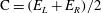
As a second method for assessing the entrainment coefficient we consider the findings of van Reeuwijk & Craske (Reference van Reeuwijk and Craske2015) in which they showed, for a time-averaged self-similar pure plume, that
 $\unicode[STIX]{x1D6FC}$
can be expressed in terms of turbulence production, energy flux and buoyancy effects. This decomposition allows a deeper physical insight of the entrainment coefficient beyond the original hypothesis provided by Morton et al. (Reference Morton, Taylor and Turner1956), i.e. that
$\unicode[STIX]{x1D6FC}$
can be expressed in terms of turbulence production, energy flux and buoyancy effects. This decomposition allows a deeper physical insight of the entrainment coefficient beyond the original hypothesis provided by Morton et al. (Reference Morton, Taylor and Turner1956), i.e. that
 $\unicode[STIX]{x1D6FC}=U_{E}/W$
, where
$\unicode[STIX]{x1D6FC}=U_{E}/W$
, where
 $U_{E}$
and
$U_{E}$
and
 $W$
are characteristic (horizontal) entrainment and (vertical) plume velocities, respectively. In particular, van Reeuwijk & Craske (Reference van Reeuwijk and Craske2015) show that
$W$
are characteristic (horizontal) entrainment and (vertical) plume velocities, respectively. In particular, van Reeuwijk & Craske (Reference van Reeuwijk and Craske2015) show that
 $\unicode[STIX]{x1D6FC}$
can be written as
$\unicode[STIX]{x1D6FC}$
can be written as
 $$\begin{eqnarray}\unicode[STIX]{x1D6FC}=-\frac{\overline{\unicode[STIX]{x1D6FF}}}{2\overline{\unicode[STIX]{x1D6FE}}}+\left(1-\frac{\overline{\unicode[STIX]{x1D703}}}{\overline{\unicode[STIX]{x1D6FE}}}\right)Ri,\end{eqnarray}$$
where
 $$\begin{eqnarray}\overline{\unicode[STIX]{x1D6FE}}=\frac{2}{\overline{W}^{3}\overline{R}^{2}}\int _{0}^{\infty }\overline{w}^{3}r\,\text{d}r,\quad \overline{\unicode[STIX]{x1D6FF}}=\frac{4}{\overline{W}^{3}\overline{R}}\int _{0}^{\infty }\overline{w^{\prime }u^{\prime }}\frac{\text{d}\overline{w}}{\text{d}r}r\,\text{d}r,\end{eqnarray}$$
 $\overline{W}=\overline{M}/\overline{Q}$
and
$\overline{W}=\overline{M}/\overline{Q}$
and
 $\overline{\unicode[STIX]{x1D703}}$
is a profile coefficient associated with non-dimensional buoyancy flux. For a pure plume the Richardson number is invariant and by definition
$\overline{\unicode[STIX]{x1D703}}$
is a profile coefficient associated with non-dimensional buoyancy flux. For a pure plume the Richardson number is invariant and by definition
 $\unicode[STIX]{x1D6E4}\equiv 1$
so
$\unicode[STIX]{x1D6E4}\equiv 1$
so
 $$\begin{eqnarray}\unicode[STIX]{x1D6E4}\equiv \frac{5}{8\unicode[STIX]{x1D6FC}}Ri=1,\end{eqnarray}$$
which combined with (3.2) gives
 $$\begin{eqnarray}\unicode[STIX]{x1D6FC}=-\frac{5\overline{\unicode[STIX]{x1D6FF}}}{16}\left(\overline{\unicode[STIX]{x1D703}}-\frac{3\overline{\unicode[STIX]{x1D6FE}}}{8}\right)^{-1}.\end{eqnarray}$$
Values of
 $\overline{\unicode[STIX]{x1D6FF}}/2\overline{\unicode[STIX]{x1D6FE}}$
calculated from our data are plotted in figure 4. From our data we are unable to provide reliable estimates of the profile coefficient
$\overline{\unicode[STIX]{x1D6FF}}/2\overline{\unicode[STIX]{x1D6FE}}$
calculated from our data are plotted in figure 4. From our data we are unable to provide reliable estimates of the profile coefficient
 $\overline{\unicode[STIX]{x1D703}}$
. However, van Reeuwijk & Craske (Reference van Reeuwijk and Craske2015) provide values for
$\overline{\unicode[STIX]{x1D703}}$
. However, van Reeuwijk & Craske (Reference van Reeuwijk and Craske2015) provide values for
 $\overline{\unicode[STIX]{x1D703}}$
(alongside those for
$\overline{\unicode[STIX]{x1D703}}$
(alongside those for
 $\overline{\unicode[STIX]{x1D6FF}}$
and
$\overline{\unicode[STIX]{x1D6FF}}$
and
 $\overline{\unicode[STIX]{x1D6FE}}$
) from six independent computations of plumes and we take the mean value they obtained
$\overline{\unicode[STIX]{x1D6FE}}$
) from six independent computations of plumes and we take the mean value they obtained
 $\overline{\unicode[STIX]{x1D703}}=0.93$
(therein table 3). The estimates of
$\overline{\unicode[STIX]{x1D703}}=0.93$
(therein table 3). The estimates of
 $\unicode[STIX]{x1D6FC}$
calculated in this manner from our data are included in figure 4. The mean values from each of our three plumes are shown and these fall within the range of values presented in van Reeuwijk & Craske (Reference van Reeuwijk and Craske2015). Moreover, the values of the entrainment coefficient, calculated in the second manner, are also
$\unicode[STIX]{x1D6FC}$
calculated in this manner from our data are included in figure 4. The mean values from each of our three plumes are shown and these fall within the range of values presented in van Reeuwijk & Craske (Reference van Reeuwijk and Craske2015). Moreover, the values of the entrainment coefficient, calculated in the second manner, are also
 $\unicode[STIX]{x1D6FC}=0.11\pm 0.01$
, identical to the values obtained from the plume equations. This demonstrates that the two different methodologies for assessing
$\unicode[STIX]{x1D6FC}=0.11\pm 0.01$
, identical to the values obtained from the plume equations. This demonstrates that the two different methodologies for assessing
 $\unicode[STIX]{x1D6FC}$
are quantitatively equivalent.
$\unicode[STIX]{x1D6FC}$
are quantitatively equivalent.

Figure 4. The values of
 $-\overline{\unicode[STIX]{x1D6FF}}/2\overline{\unicode[STIX]{x1D6FE}}$
(grey) and
$-\overline{\unicode[STIX]{x1D6FF}}/2\overline{\unicode[STIX]{x1D6FE}}$
(grey) and
 $\unicode[STIX]{x1D6FC}$
(black) calculated from our data, plotted against the vertical distance from the virtual origin
$\unicode[STIX]{x1D6FC}$
(black) calculated from our data, plotted against the vertical distance from the virtual origin
 $z/r_{0}$
. The mean values for each experiment taking all data at all heights plotted are shown in the legend. The dashed lines show the minimum and maximum values of
$z/r_{0}$
. The mean values for each experiment taking all data at all heights plotted are shown in the legend. The dashed lines show the minimum and maximum values of
 $\unicode[STIX]{x1D6FC}$
presented in van Reeuwijk & Craske (Reference van Reeuwijk and Craske2015).
$\unicode[STIX]{x1D6FC}$
presented in van Reeuwijk & Craske (Reference van Reeuwijk and Craske2015).
4 Results and discussion
In order to provide novel insights for the dynamics that arises within turbulent plumes we combine measurements of the velocity field with data for the edges of the scalar field. We do so using two distinct methods, the first of which exploits the Heaviside step function (§ 4.2) and the second establishes a coordinate system which follows the meandering fluctuating plume (§ 4.3). In order to set these methods in context we first examine results following directly from our measurements of the scalar edges.
4.1 The statistics of the scalar edges

Figure 5. Histograms of the location of the centre, left- and right-hand edge of the plume scalar field and the magnitude of the width of the plume scalar field. All distances have been normalised by the time average of the local half-width of the scalar edges of the plume,
 $\overline{R_{p}}$
. The histograms contain observations from each of the three plumes, from both edge-detection algorithms and at all heights for which reliable data were obtained – in excess of
$\overline{R_{p}}$
. The histograms contain observations from each of the three plumes, from both edge-detection algorithms and at all heights for which reliable data were obtained – in excess of
 $6\times 10^{7}$
observations of each statistic. The best-fit Gaussian distribution is overlaid on each histogram.
$6\times 10^{7}$
observations of each statistic. The best-fit Gaussian distribution is overlaid on each histogram.
The radial location of the left-hand and right-hand edges of the plume fluid are plotted in figure 5, in which all distances have been normalised on the time-averaged half-width of the scalar field edges
 $\overline{R_{p}}$
. Both are well approximated by the normalised Gaussian distributions
$\overline{R_{p}}$
. Both are well approximated by the normalised Gaussian distributions
 $E_{L}\sim N\,(\unicode[STIX]{x1D707}=-1,\unicode[STIX]{x1D70E}^{2}=0.072)$
and
$E_{L}\sim N\,(\unicode[STIX]{x1D707}=-1,\unicode[STIX]{x1D70E}^{2}=0.072)$
and
 $E_{R}\sim N\,(\unicode[STIX]{x1D707}=1,\unicode[STIX]{x1D70E}^{2}=0.070)$
for the left- and right-hand edges, respectively, where
$E_{R}\sim N\,(\unicode[STIX]{x1D707}=1,\unicode[STIX]{x1D70E}^{2}=0.070)$
for the left- and right-hand edges, respectively, where
 $\unicode[STIX]{x1D707}$
denotes the mean and
$\unicode[STIX]{x1D707}$
denotes the mean and
 $\unicode[STIX]{x1D70E}$
the standard deviation. From the instantaneous locations of the left- and right-hand edges we define the instantaneous centre of the plume fluid and the width
$\unicode[STIX]{x1D70E}$
the standard deviation. From the instantaneous locations of the left- and right-hand edges we define the instantaneous centre of the plume fluid and the width
 $2R_{p}$
which approximately follow the normalised Gaussian distributions
$2R_{p}$
which approximately follow the normalised Gaussian distributions
 $\text{C}\sim N\,(0,0.036)$
and
$\text{C}\sim N\,(0,0.036)$
and
 $2R_{p}\sim N\,(2,0.140)$
, respectively.
$2R_{p}\sim N\,(2,0.140)$
, respectively.
The relatively small variation in the central point,
 $\text{C}$
, highlights that meanders of the plume centreline are small in comparison to the fluctuations in the plume width; where by fluctuations we refer to variations about the mean. Moreover, since
$\text{C}$
, highlights that meanders of the plume centreline are small in comparison to the fluctuations in the plume width; where by fluctuations we refer to variations about the mean. Moreover, since
 $\text{C}=(E_{L}+E_{R})/2$
and
$\text{C}=(E_{L}+E_{R})/2$
and
 $2R_{p}=E_{R}-E_{L}$
it follows from the observed distributions that the covariance,
$2R_{p}=E_{R}-E_{L}$
it follows from the observed distributions that the covariance,
 $\text{cov}(E_{L},E_{R})$
, is not statistically significantly different from zero. Hence, the location of the left- and right-hand edges of the plume are not correlated. Such a finding implies an absence of coherent structures forming across the full width of the plume, since such structures would simultaneously affect the locations of the left- and right-hand edges and result in their locations being correlated.
$\text{cov}(E_{L},E_{R})$
, is not statistically significantly different from zero. Hence, the location of the left- and right-hand edges of the plume are not correlated. Such a finding implies an absence of coherent structures forming across the full width of the plume, since such structures would simultaneously affect the locations of the left- and right-hand edges and result in their locations being correlated.
4.2 Interrogating the velocity field using Heaviside step functions

Figure 6. The radial distributions of vertical (solid lines) and horizontal (dashed lines) velocities, in the scaled Eulerian plume coordinate. The velocities are conditioned on the presence of plume fluid or ambient fluid, plotted at radial locations where the probability of observation exceeded 3 %. The data show that fluid inside the plume moves vertically faster (by
 $0.1{-}0.2\overline{w_{c}}$
) than ambient fluid at the same vertical location. Ambient fluid is accelerated both horizontally and vertically in the regions
$0.1{-}0.2\overline{w_{c}}$
) than ambient fluid at the same vertical location. Ambient fluid is accelerated both horizontally and vertically in the regions
 $r/\overline{R_{p}}\approx \pm 0.5$
–
$r/\overline{R_{p}}\approx \pm 0.5$
–
 $\pm 1.0$
. The velocity profile observed when engulfed fluid is present shows that much of the vertical acceleration occurs as ambient fluid is engulfed, with engulfed fluid travelling at approximately 80 % of the velocity of plume fluid locally.
$\pm 1.0$
. The velocity profile observed when engulfed fluid is present shows that much of the vertical acceleration occurs as ambient fluid is engulfed, with engulfed fluid travelling at approximately 80 % of the velocity of plume fluid locally.

Figure 7. The radial distributions of (a) vertical (solid lines) and horizontal (dashed lines) velocity fluctuations and (b) Reynolds stresses, in the Eulerian plume coordinate. Observations are conditioned on presence of the plume or the ambient (colour scheme as in figure 6). The data show large Reynolds stresses in ambient fluid when in the regions
 $r/\overline{R_{p}}\approx \pm 0.5$
–
$r/\overline{R_{p}}\approx \pm 0.5$
–
 $\pm 0.8$
.
$\pm 0.8$
.
Given that the extent of the meandering is small relative to the width of the plume (figure 5) there will be regions near the centreline where, almost always, plume fluid will be present. Conversely, sufficiently far from the centreline, no plume fluid will ever be present. The balance of these probabilities alters at intermediate radial locations. At a fixed location in these intermediate regions, it is possible to make conditional observations, based on whether fluid at that location is instantaneously inside or outside the plume, which are statistically representative of these two states. As such, we couple our measurements of the velocity field with our data for the edges of the scalar field via a plume step function which is unity within the plume and zero outside and is defined by
 $$\begin{eqnarray}H_{in}(r,z,t)=H_{s}[r-E_{L}(z,t)]-H_{s}[r-E_{R}(z,t)],\end{eqnarray}$$
where
 $H_{s}$
is the Heaviside step function,
$H_{s}$
is the Heaviside step function,
 $H_{S}(x)=0$
, for
$H_{S}(x)=0$
, for
 $x<0$
and
$x<0$
and
 $H_{S}(x)=1$
, for
$H_{S}(x)=1$
, for
 $x\geqslant 0$
. We can then determine the time-averaged vertical velocity, at a given location, conditional on being inside,
$x\geqslant 0$
. We can then determine the time-averaged vertical velocity, at a given location, conditional on being inside,
 $\overline{w_{in}}$
or outside,
$\overline{w_{in}}$
or outside,
 $\overline{w_{out}}$
, the plume by defining
$\overline{w_{out}}$
, the plume by defining
 $$\begin{eqnarray}\overline{w_{in}(r,z)}=\frac{1}{T_{in}}\int _{0}^{T}H_{in}w(r,z,t)\,\text{d}t\quad \text{and}\quad \overline{w_{out}(r,z)}=\frac{1}{T_{out}}\int _{0}^{T}(1-H_{in})w(r,z,t)\,\text{d}t,\end{eqnarray}$$
where
 $T_{in}(r,z)$
and
$T_{in}(r,z)$
and
 $T_{out}(r,z)$
correspond to the total amount of time fluid at a given location is inside and outside the plume, respectively. We define the horizontal velocities conditional on being inside
$T_{out}(r,z)$
correspond to the total amount of time fluid at a given location is inside and outside the plume, respectively. We define the horizontal velocities conditional on being inside
 $\overline{u_{in}}$
or outside
$\overline{u_{in}}$
or outside
 $\overline{u_{out}}$
the plume in an equivalent manner.
$\overline{u_{out}}$
the plume in an equivalent manner.
Figure 6 shows the radial variation of the vertical (solid lines) and horizontal (dashed lines) velocities. Data obtained from the three different plumes at 18 different heights and plume edges calculated from both edge-detection algorithms (see § 2.2) are plotted in each of figures 6, 7, 9–11 and 13–15. Black curves mark the full time-averaged data (akin to the black curves in figure 2), overlaid (in blue) are the velocities when inside the plume and (in grey) the velocities when outside the plume. Data are plotted only in regions where the probability of observing a given state exceeds 3 % (equivalent to approximately 400 observations). The probability exceeding 3 % that the radial location is inside the plume occurs for
 $|r|\lesssim 1.5\overline{R_{p}}$
and the probability exceeding 3 % that the radial location is outside the plume occurs for
$|r|\lesssim 1.5\overline{R_{p}}$
and the probability exceeding 3 % that the radial location is outside the plume occurs for
 $|r|\gtrsim 0.5\overline{R_{p}}$
. Note that, while we choose to scale the radial coordinate by the plume half-width defined by the edges of the scalar field
$|r|\gtrsim 0.5\overline{R_{p}}$
. Note that, while we choose to scale the radial coordinate by the plume half-width defined by the edges of the scalar field
 $\overline{R_{p}}$
, notionally identical plots would be produced should the radial coordinate be scaled by the top-hat half-width,
$\overline{R_{p}}$
, notionally identical plots would be produced should the radial coordinate be scaled by the top-hat half-width,
 $\overline{R}$
since our measurements show that
$\overline{R}$
since our measurements show that
 $\overline{R_{p}}\approx \overline{R}$
(§ 4.4).
$\overline{R_{p}}\approx \overline{R}$
(§ 4.4).
Figure 6 shows that at a given radial location the vertical velocity is significantly larger inside the plume compared with the velocity outside (an increase of approximately
 $0.1\overline{w_{c}}$
–
$0.1\overline{w_{c}}$
–
 $0.2\overline{w_{c}}$
). This indicates that, as expected, fluid is accelerated vertically as it transitions from outside to inside the plume i.e. transported across the plume envelope – while, at first thought, this result may seem trivial we return to its full implications in § 4.2.2. Figure 6 also indicates that when ambient fluid outside the plume is drawn radially inwards towards the plume, but still remains outside the plume in the region
$0.2\overline{w_{c}}$
). This indicates that, as expected, fluid is accelerated vertically as it transitions from outside to inside the plume i.e. transported across the plume envelope – while, at first thought, this result may seem trivial we return to its full implications in § 4.2.2. Figure 6 also indicates that when ambient fluid outside the plume is drawn radially inwards towards the plume, but still remains outside the plume in the region
 $|r|<\overline{R_{p}}$
, then this fluid experiences significant accelerations both vertically and radially (with radial velocities reaching
$|r|<\overline{R_{p}}$
, then this fluid experiences significant accelerations both vertically and radially (with radial velocities reaching
 $|\overline{u_{out}}|\approx 0.15\overline{w_{c}}$
being approximately five times larger than the largest horizontal velocities observed in the mean). From observations in this reference frame it is not clear whether this acceleration is driven by short-range viscous effects at the plume edge or longer-range pressure gradients, since the distance between the fluid outside the plume and the plume edge at a given instant is unknown. We will show that this acceleration must result from long-range pressure gradients in § 4.3.
$|\overline{u_{out}}|\approx 0.15\overline{w_{c}}$
being approximately five times larger than the largest horizontal velocities observed in the mean). From observations in this reference frame it is not clear whether this acceleration is driven by short-range viscous effects at the plume edge or longer-range pressure gradients, since the distance between the fluid outside the plume and the plume edge at a given instant is unknown. We will show that this acceleration must result from long-range pressure gradients in § 4.3.
Figure 7(a) shows the root mean square of the velocity fluctuations, defined, for example, by
 $w_{rms}^{\prime }(r,z)=[(1/T)\int _{0}^{T}[w^{\prime }(r,z,t)]^{2}\,\text{d}t]^{1/2}$
, where
$w_{rms}^{\prime }(r,z)=[(1/T)\int _{0}^{T}[w^{\prime }(r,z,t)]^{2}\,\text{d}t]^{1/2}$
, where
 $w^{\prime }(r,z,t)=w(r,z,t)-\overline{w(r,z)}$
. The full time average of the vertical velocity fluctuations shows a bi-modal peak, qualitatively similar to observations in previous studies of jets (e.g. Shabbir & George Reference Shabbir and George1994) and quantitatively similar to previous observations of plumes (van Reeuwijk et al.
Reference van Reeuwijk, Salizzoni, Hunt and Craske2016). We find that the vertical velocity fluctuations within fluid inside the plume exhibit an approximately flat peak for
$w^{\prime }(r,z,t)=w(r,z,t)-\overline{w(r,z)}$
. The full time average of the vertical velocity fluctuations shows a bi-modal peak, qualitatively similar to observations in previous studies of jets (e.g. Shabbir & George Reference Shabbir and George1994) and quantitatively similar to previous observations of plumes (van Reeuwijk et al.
Reference van Reeuwijk, Salizzoni, Hunt and Craske2016). We find that the vertical velocity fluctuations within fluid inside the plume exhibit an approximately flat peak for
 $|r|\lesssim \overline{R_{p}}$
. The vertical velocity fluctuations for fluid outside the plume exhibit a sharp peak as
$|r|\lesssim \overline{R_{p}}$
. The vertical velocity fluctuations for fluid outside the plume exhibit a sharp peak as
 $|r|\rightarrow 0.5\overline{R_{p}}$
, indicating that large velocity fluctuations occur in ambient fluid when it is found relatively close to the centreline, although the occurrence of such events is relatively rare. Mean profiles of the Reynolds stress, figure 7(b), show peaks (of
$|r|\rightarrow 0.5\overline{R_{p}}$
, indicating that large velocity fluctuations occur in ambient fluid when it is found relatively close to the centreline, although the occurrence of such events is relatively rare. Mean profiles of the Reynolds stress, figure 7(b), show peaks (of
 $\overline{u^{\prime }w^{\prime }}/\overline{w_{c}}^{2}\approx 0.015$
) at
$\overline{u^{\prime }w^{\prime }}/\overline{w_{c}}^{2}\approx 0.015$
) at
 $r\approx 0.5\overline{R_{p}}$
which drop off rapidly at larger radial locations, e.g.
$r\approx 0.5\overline{R_{p}}$
which drop off rapidly at larger radial locations, e.g.
 $\overline{u^{\prime }w^{\prime }}/\overline{w_{c}}^{2}\leqslant 0.001$
for
$\overline{u^{\prime }w^{\prime }}/\overline{w_{c}}^{2}\leqslant 0.001$
for
 $|r|\gtrsim 1.2\overline{R_{p}}$
– these mean Reynolds stress profiles are similar to those reported in previous studies of plumes (e.g. van Reeuwijk et al.
Reference van Reeuwijk, Salizzoni, Hunt and Craske2016). However, for fluid inside the plume the magnitude of the Reynolds stress remains close to these peak values at far larger radial locations, e.g.
$|r|\gtrsim 1.2\overline{R_{p}}$
– these mean Reynolds stress profiles are similar to those reported in previous studies of plumes (e.g. van Reeuwijk et al.
Reference van Reeuwijk, Salizzoni, Hunt and Craske2016). However, for fluid inside the plume the magnitude of the Reynolds stress remains close to these peak values at far larger radial locations, e.g.
 $\overline{u_{in}^{\prime }w_{in}^{\prime }}/\overline{w_{c}}^{2}\approx 0.015$
at
$\overline{u_{in}^{\prime }w_{in}^{\prime }}/\overline{w_{c}}^{2}\approx 0.015$
at
 $r\approx 1.2\overline{R_{p}}$
. Outside the plume, when ambient fluid is relatively close to the centreline the Reynolds stress exhibits a sharp peak, reaching
$r\approx 1.2\overline{R_{p}}$
. Outside the plume, when ambient fluid is relatively close to the centreline the Reynolds stress exhibits a sharp peak, reaching
 $\overline{u_{out}^{\prime }w_{out}^{\prime }}/\overline{w_{c}}^{2}\gtrsim 0.03$
at
$\overline{u_{out}^{\prime }w_{out}^{\prime }}/\overline{w_{c}}^{2}\gtrsim 0.03$
at
 $r\approx 0.5\overline{R_{p}}$
. These peaks in the Reynolds stress suggest that when ambient fluid is relatively close to the centreline the local turbulence production is at its largest, presumably as this ambient fluid is about to be entrained into the plume.
$r\approx 0.5\overline{R_{p}}$
. These peaks in the Reynolds stress suggest that when ambient fluid is relatively close to the centreline the local turbulence production is at its largest, presumably as this ambient fluid is about to be entrained into the plume.
Figure 6 indicates that the vertical velocities in the ambient fluid can be significant, for example
 $\overline{w_{out}}\approx 0.4\overline{w_{c}}$
for ambient fluid at
$\overline{w_{out}}\approx 0.4\overline{w_{c}}$
for ambient fluid at
 $r\approx 0.5\overline{R_{p}}$
, suggesting that the vertical volume (mass) transport within the ambient fluid outside the plume, might also be significant. We calculate an estimate of the vertical volume flux inside the plume from
$r\approx 0.5\overline{R_{p}}$
, suggesting that the vertical volume (mass) transport within the ambient fluid outside the plume, might also be significant. We calculate an estimate of the vertical volume flux inside the plume from
 $$\begin{eqnarray}\overline{Q_{in}(z)}=\frac{1}{T}\int _{-\infty }^{\infty }r\int _{0}^{T}H_{in}w(r,z,t)\,\text{d}t\,\text{d}r,\end{eqnarray}$$
and hence obtain an estimate for the transport outside the plume from
 $\overline{Q_{out}(z)}=\overline{Q(z)}-\overline{Q_{in}(z)}$
. Figure 8 shows these values from the three plumes and shows that, as expected for a self-similar flow, the proportion of the vertical transport outside the plume is constant with height and constitutes approximately 5 % of the total vertical transport (
$\overline{Q_{out}(z)}=\overline{Q(z)}-\overline{Q_{in}(z)}$
. Figure 8 shows these values from the three plumes and shows that, as expected for a self-similar flow, the proportion of the vertical transport outside the plume is constant with height and constitutes approximately 5 % of the total vertical transport (
 $\overline{Q_{out}(z)}/\overline{Q(z)}=0.046\pm 0.006$
, where the tolerances indicate the standard deviation within our measurements).
$\overline{Q_{out}(z)}/\overline{Q(z)}=0.046\pm 0.006$
, where the tolerances indicate the standard deviation within our measurements).

Figure 8. The dimensionless volume fluxes (thick lines) when eddies are present (green) and absent (red) relative to the mean, i.e.
 $\overline{Q_{e}}/\overline{Q}$
and
$\overline{Q_{e}}/\overline{Q}$
and
 $\overline{Q_{n}}/\overline{Q}$
, respectively. The proportion of the vertical transport occurring outside the plume are also shown for each of the three states, i.e. mean
$\overline{Q_{n}}/\overline{Q}$
, respectively. The proportion of the vertical transport occurring outside the plume are also shown for each of the three states, i.e. mean
 $\overline{Q_{out}}/\overline{Q}$
(thin black lines), eddy present
$\overline{Q_{out}}/\overline{Q}$
(thin black lines), eddy present
 $\overline{Q_{(out,e)}}/\overline{Q_{e}}$
(thin green lines) and absent
$\overline{Q_{(out,e)}}/\overline{Q_{e}}$
(thin green lines) and absent
 $\overline{Q_{(out,n)}}/\overline{Q_{n}}$
(thin red lines).
$\overline{Q_{(out,n)}}/\overline{Q_{n}}$
(thin red lines).

Figure 9. Radial distributions of vertical (solid lines) and horizontal (dashed lines) velocities, in the scaled plume coordinate. Observations of the velocities conditioned on the local presence of large-scale coherent structures are included. Vertical lines mark the time-averaged position of the plume edge in the mean (black), eddy present (green), eddy absent (red). The data show significant vertical velocities outside the plume when eddies are absent and almost no vertical flow outside the plume when eddies are present.
4.2.1 The velocity field and fluxes when eddies are present and absent
Having identified that approximately 5 % of the vertical volume flux is associated with flow outside the plume, we investigate the role of the large-scale coherent structures on this transport and, more broadly, their role in the process of turbulent entrainment. To do so, we examine our measurements of the velocity field conditional on whether one might reasonably expect a large-scale coherent structure (eddy) to be locally present or absent at a given height. We reason that the presence of a large-scale coherent structure (eddy) results in an increase in the local width of the flow – a similar reasoning enabled the evolution of these structures to be successfully tracked in turbulent plumes (Burridge et al.
Reference Burridge, Partridge and Linden2016). As such, the presence of an eddy within the plume is inferred when the local plume width is greater than the mean plume width by more than one standard deviation,
 $\unicode[STIX]{x1D70E}_{R}(z)$
. Conversely, we infer that no eddy is present (eddy absent) when the local plume width is less than the mean plume width by more than one standard deviation. Note that the threshold used to define eddy present and absent events, i.e.
$\unicode[STIX]{x1D70E}_{R}(z)$
. Conversely, we infer that no eddy is present (eddy absent) when the local plume width is less than the mean plume width by more than one standard deviation. Note that the threshold used to define eddy present and absent events, i.e.
 $\pm 1\times \unicode[STIX]{x1D70E}_{R}(z)$
, is in some sense arbitrary. However, our results are not dramatically affected if the threshold is premultiplied by a value differing moderately from unity. Moreover, our choice of a single standard deviation ensured that we were able to average a statistically significant sample size. With our choice of threshold eddy present and eddy absent events constituted approximately 30 % of all observations (figure 5).
$\pm 1\times \unicode[STIX]{x1D70E}_{R}(z)$
, is in some sense arbitrary. However, our results are not dramatically affected if the threshold is premultiplied by a value differing moderately from unity. Moreover, our choice of a single standard deviation ensured that we were able to average a statistically significant sample size. With our choice of threshold eddy present and eddy absent events constituted approximately 30 % of all observations (figure 5).
We define eddy present,
 $H_{e}(z,t)$
, and eddy absent,
$H_{e}(z,t)$
, and eddy absent,
 $H_{n}(z,t)$
, step functions by
$H_{n}(z,t)$
, step functions by
 $$\begin{eqnarray}H_{e}=\left\{\begin{array}{@{}l@{}}0\text{ for }R_{p}(z,t)<\overline{R_{p}(z)}+\unicode[STIX]{x1D70E}_{R}(z)\\ 1\text{ for }R_{p}(z,t)\geqslant \overline{R_{p}(z)}+\unicode[STIX]{x1D70E}_{R}(z)\end{array}\right.\quad \text{and}\quad H_{n}=\left\{\begin{array}{@{}l@{}}1,R_{p}(z,t)<\overline{R_{p}(z)}-\unicode[STIX]{x1D70E}_{R}(z)\\ 0,R_{p}(z,t)\geqslant \overline{R_{p}(z)}-\unicode[STIX]{x1D70E}_{R}(z),\end{array}\right.\end{eqnarray}$$
respectively. From (4.4) we can estimate the total volume fluxes
 $\overline{Q_{e}}$
and
$\overline{Q_{e}}$
and
 $\overline{Q_{n}}$
in the presence and absence of eddies, respectively, by for example
$\overline{Q_{n}}$
in the presence and absence of eddies, respectively, by for example
 $$\begin{eqnarray}\overline{Q_{e}(z)}=\frac{1}{T}\int _{-\infty }^{\infty }r\int _{0}^{T}H_{e}w(r,z,t)\,\text{d}t\,\text{d}r,\end{eqnarray}$$
with equivalent expressions for
 $\overline{Q_{n}}$
, and further determine the fluxes inside and outside the plume in each state, by for example
$\overline{Q_{n}}$
, and further determine the fluxes inside and outside the plume in each state, by for example
 $$\begin{eqnarray}\overline{Q_{(in,e)}(z)}=\frac{1}{T}\int _{-\infty }^{\infty }r\int _{0}^{T}H_{in}H_{e}w(r,z,t)\,\text{d}t\,\text{d}r.\end{eqnarray}$$
with equivalent expressions for
 $\overline{Q_{(out,e)}}$
.
$\overline{Q_{(out,e)}}$
.
Figure 8 shows the resulting vertical volume fluxes in the presence and absence of eddies. The figure shows that the total vertical transport is increased or decreased by approximately 9 % when eddies are present or absent, respectively, with
 $\overline{Q_{e}(z)}/\overline{Q(z)}=1.085\pm 0.013$
and
$\overline{Q_{e}(z)}/\overline{Q(z)}=1.085\pm 0.013$
and
 $\overline{Q_{n}(z)}/\overline{Q(z)}=0.908\pm 0.006$
. More insightful are the fluxes outside the plume in the presence and absence of eddies. Figure 8 further shows that when large-scale coherent structures are present almost all of the vertical transport occurs inside the plume,
$\overline{Q_{n}(z)}/\overline{Q(z)}=0.908\pm 0.006$
. More insightful are the fluxes outside the plume in the presence and absence of eddies. Figure 8 further shows that when large-scale coherent structures are present almost all of the vertical transport occurs inside the plume,
 $\overline{Q_{(out,e)}}/\overline{Q_{e}}=-0.001\pm 0.009$
. Conversely, when no eddies are present the vertical transport outside the plume is significant,
$\overline{Q_{(out,e)}}/\overline{Q_{e}}=-0.001\pm 0.009$
. Conversely, when no eddies are present the vertical transport outside the plume is significant,
 $\overline{Q_{(out,n)}}/\overline{Q_{n}}=0.135\pm 0.010$
. Such findings clearly illustrate the importance of coherent structures for the turbulent entrainment by plumes. At ‘eddy-present’ events there is virtually no vertical transport outside the plume while between eddies this transport is significant, so ambient fluid must be accelerated vertically outside the plume between eddy present events.
$\overline{Q_{(out,n)}}/\overline{Q_{n}}=0.135\pm 0.010$
. Such findings clearly illustrate the importance of coherent structures for the turbulent entrainment by plumes. At ‘eddy-present’ events there is virtually no vertical transport outside the plume while between eddies this transport is significant, so ambient fluid must be accelerated vertically outside the plume between eddy present events.
We now examine the radial profiles of velocity, in a fixed Eulerian frame, conditional on the presence and absence of large-scale coherent structures. However, given that the profiles observed in an Eulerian frame of reference take no account of the spatial extent or location of the radial distribution at a given instant, interpretation of these data requires care. For example, the profiles in figure 9 show larger vertical velocities when eddies are present but in effect this is merely an alternative illustration of the associated larger vertical volumes fluxes. The vertical lines in figure 9, however, mark the time-averaged position of the plume edge in each of the three states and suggest that the vertical velocities near the plume edge are significantly different depending on whether an eddy is locally present or not. In order to provide more physical insight we re-examine these profiles in § 4.3 within a plume coordinate that follows the meanders and fluctuations in width of the plume. However, before moving on, we note that observations in the fixed Eulerian coordinate indicate that changes in the vertical velocity fluctuations between the three states (figure 10 a) appear to produce greater Reynolds stresses (figure 10 b) in the absence of eddies. If velocity gradients remain broadly similar between the three states, then these peaks imply that the local turbulence production is greatest at locations between eddies. This supports our findings regarding the Reynolds stresses in § 4.2 and our suggestion that the local turbulence production is greatest as ambient fluid is being entrained within the plume. However, these findings should be compared with observations in the plume coordinate (§ 4.3).

Figure 10. Radial distributions of (a) vertical (solid lines) and horizontal (dashed lines) velocity fluctuations and (b) Reynolds stresses, in the scaled plume coordinate. Observations conditioned on the local presence of large-scale coherent structures are included. The data show Reynolds stresses of slightly greater magnitude when coherent structures are absent.

Figure 11. The probability, at a given radial location, of being within the plume (thin black lines), finding mixed fluid (thick grey lines) and finding engulfed fluid (thick black lines), from ensemble averages of the three plumes over all heights for which reliable data were obtained. Solid lines mark the results from the standard edge-detection algorithm and dashed lines those from the alternative algorithm.
4.2.2 The distribution, velocity profile and fluxes of engulfed fluid
We have shown that significant vertical transport (approximately 14 %) occurs outside the plume at locations between the large-scale coherent structures in the plume. In order to shed light on the process through which this ambient fluid is entrained and ultimately mixed within the plume we now consider the fluid inside the plume envelope. In accordance with (4.1), we define the plume envelope as the flow between the instantaneous left- and right-hand edges of the plume scalar field (§ 2.2), i.e. within the loci of the instantaneous plume edges. Then the probability of being within the plume envelope at a given radial location is defined by
 $P_{in}(r,z)=(1/T)\int _{0}^{T}H_{in}(r,z,t)\,\text{d}t$
. This probability distribution exhibits a broad single peak (see the thin black curve in figure 11), indicating that central regions,
$P_{in}(r,z)=(1/T)\int _{0}^{T}H_{in}(r,z,t)\,\text{d}t$
. This probability distribution exhibits a broad single peak (see the thin black curve in figure 11), indicating that central regions,
 $-0.5\overline{R_{p}}\lesssim r\lesssim 0.5\overline{R_{p}}$
, are almost certain to be within the plume envelope. However, as has been reported for turbulent jets (Westerweel et al.
Reference Westerweel, Fukushima, Pedersen and Hunt2009), we find that there are pockets of unmixed ambient fluid inside the plume envelope which, under our definition (§ 1), have been engulfed as part of the process of turbulent entrainment. We define engulfed fluid as any fluid within the plume envelope which exhibits a lower scalar concentration than that of the fluid at the instantaneous edge of the plume. Naturally, the concentration of scalar (dye) at any instant may be different at the left,
$-0.5\overline{R_{p}}\lesssim r\lesssim 0.5\overline{R_{p}}$
, are almost certain to be within the plume envelope. However, as has been reported for turbulent jets (Westerweel et al.
Reference Westerweel, Fukushima, Pedersen and Hunt2009), we find that there are pockets of unmixed ambient fluid inside the plume envelope which, under our definition (§ 1), have been engulfed as part of the process of turbulent entrainment. We define engulfed fluid as any fluid within the plume envelope which exhibits a lower scalar concentration than that of the fluid at the instantaneous edge of the plume. Naturally, the concentration of scalar (dye) at any instant may be different at the left,
 $c_{L}(z,t)$
, and right,
$c_{L}(z,t)$
, and right,
 $c_{R}(z,t)$
, hand edges of the plume. To test the sensitivity of our findings to the precise dye concentration threshold,
$c_{R}(z,t)$
, hand edges of the plume. To test the sensitivity of our findings to the precise dye concentration threshold,
 $c_{T}(z,t)$
, used to determine engulfed fluid we examined three alternative methods to determine the threshold namely: (i) the minimum of the concentration at the two edges, i.e.
$c_{T}(z,t)$
, used to determine engulfed fluid we examined three alternative methods to determine the threshold namely: (i) the minimum of the concentration at the two edges, i.e.
 $c_{T}(z,t)=\text{min}[c_{L}(z,t),c_{R}(z,t)]$
, (ii) the maximum of the concentration at the two edges, i.e.
$c_{T}(z,t)=\text{min}[c_{L}(z,t),c_{R}(z,t)]$
, (ii) the maximum of the concentration at the two edges, i.e.
 $c_{T}(z,t)=\text{max}[c_{L}(z,t),c_{R}(z,t)]$
and (iii) the concentration determined by the (radially) closest edge, i.e.
$c_{T}(z,t)=\text{max}[c_{L}(z,t),c_{R}(z,t)]$
and (iii) the concentration determined by the (radially) closest edge, i.e.
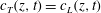 $c_{T}(z,t)=c_{L}(z,t)$
for
$c_{T}(z,t)=c_{L}(z,t)$
for
 $r_{p}<0$
and
$r_{p}<0$
and
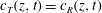 $c_{T}(z,t)=c_{R}(z,t)$
for
$c_{T}(z,t)=c_{R}(z,t)$
for
 $r_{p}\geqslant 0$
. We report results determined when engulfed fluid is defined by criterion (iii) and we include tolerances to indicate the maximum variation in our results should we have chosen criteria (i) or (ii). Moreover, should our experiments have resolved the scalar field to the precision of the Batchelor length scale then some variation in the detection of engulfed fluid could be expected since diffusion would act to smear the scalar edges of the plume over a length scale larger than one pixel. However, we expect that these variations would fall well within the tolerances indicated for our results.
$r_{p}\geqslant 0$
. We report results determined when engulfed fluid is defined by criterion (iii) and we include tolerances to indicate the maximum variation in our results should we have chosen criteria (i) or (ii). Moreover, should our experiments have resolved the scalar field to the precision of the Batchelor length scale then some variation in the detection of engulfed fluid could be expected since diffusion would act to smear the scalar edges of the plume over a length scale larger than one pixel. However, we expect that these variations would fall well within the tolerances indicated for our results.
In order to examine the location and fluxes of engulfed fluid we define an ambient fluid step function
 $$\begin{eqnarray}H_{amb}(r,z,t)=\left\{\begin{array}{@{}l@{}}1\text{ for }c(r,z,t)<c_{T}(z,t)\\ 0\text{ for }c(r,z,t)\geqslant c_{T}(z,t),\end{array}\right.\end{eqnarray}$$
where
 $c(r,z,t)$
is the local buoyancy scalar concentration. From (4.7) we can determine the presence of engulfed fluid from
$c(r,z,t)$
is the local buoyancy scalar concentration. From (4.7) we can determine the presence of engulfed fluid from
 $H_{eng}(r,z,t)=H_{in}(r,z,t)\times H_{amb}(r,z,t)$
, and mixed plume fluid,
$H_{eng}(r,z,t)=H_{in}(r,z,t)\times H_{amb}(r,z,t)$
, and mixed plume fluid,
 $H_{mix}(r,z,t)=H_{in}(r,z,t)[1-H_{amb}(r,z,t)]$
. Figure 11 includes the observed probability distributions of engulfed fluid (thick black curves) and mixed fluid (thick grey curves), e.g.
$H_{mix}(r,z,t)=H_{in}(r,z,t)[1-H_{amb}(r,z,t)]$
. Figure 11 includes the observed probability distributions of engulfed fluid (thick black curves) and mixed fluid (thick grey curves), e.g.
 $P_{eng}(r,z)=(1/T)\int _{0}^{T}H_{eng}(r,z,t)\,\text{d}t$
. We note that the qualitative shape of the data shown in figure 11 is unaffected by the choice of engulfed fluid threshold criterion. The engulfed fluid exhibits a bi-modal distribution with the probabilities of finding engulfed fluid peaking at value of almost
$P_{eng}(r,z)=(1/T)\int _{0}^{T}H_{eng}(r,z,t)\,\text{d}t$
. We note that the qualitative shape of the data shown in figure 11 is unaffected by the choice of engulfed fluid threshold criterion. The engulfed fluid exhibits a bi-modal distribution with the probabilities of finding engulfed fluid peaking at value of almost
 $20\,\%\pm 2\,\%$
, located just inside the time-averaged locations of the edges.
$20\,\%\pm 2\,\%$
, located just inside the time-averaged locations of the edges.

Figure 12. The proportion of the vertical transport which occurs as engulfed (unmixed) fluid within the plume envelope for each of the three states: mean
 $\overline{Q_{eng}}/\overline{Q}$
, eddy present
$\overline{Q_{eng}}/\overline{Q}$
, eddy present
 $\overline{Q_{(eng,e)}}/\overline{Q_{e}}$
and absent
$\overline{Q_{(eng,e)}}/\overline{Q_{e}}$
and absent
 $\overline{Q_{(eng,n)}}/\overline{Q_{n}}$
.
$\overline{Q_{(eng,n)}}/\overline{Q_{n}}$
.
We can examine the radial distribution of velocity within engulfed fluid in a manner similar to that described in § 4.2 for fluid inside and outside the plume. We define the velocity
 $\overline{w_{eng}}$
within engulfed fluid by
$\overline{w_{eng}}$
within engulfed fluid by
 $$\begin{eqnarray}\overline{w_{eng}(r,z)}=\frac{1}{T_{eng}}\int _{0}^{T}H_{eng}w(r,z,t)\,\text{d}t,\end{eqnarray}$$
where
 $T_{eng}=T_{eng}(r,w)$
is the total time for which engulfed fluid is observed at a given location. The radial profiles of
$T_{eng}=T_{eng}(r,w)$
is the total time for which engulfed fluid is observed at a given location. The radial profiles of
 $\overline{w_{eng}}$
are included in figure 6 (magenta curves). The velocity of engulfed fluid is fairly close to (approximately 80 % of) the mean velocity within the plume. This indicates that there is significant vertical acceleration as ambient fluid is transported across the plume envelope by engulfment. There must also then be a more moderate vertical acceleration during the mixing process (at smaller scales).
$\overline{w_{eng}}$
are included in figure 6 (magenta curves). The velocity of engulfed fluid is fairly close to (approximately 80 % of) the mean velocity within the plume. This indicates that there is significant vertical acceleration as ambient fluid is transported across the plume envelope by engulfment. There must also then be a more moderate vertical acceleration during the mixing process (at smaller scales).
Comparing the magnitude of the vertical fluxes of transport outside the plume with those of engulfed fluid within the plume provides a measure of the proportion of ambient fluid that is engulfed into the plume envelope. One might be tempted to try to estimate the flux of engulfed fluid by evaluating the integral
 $$\begin{eqnarray}I=\int _{-\infty }^{\infty }P_{eng}r\overline{w(r,z)}\,\text{d}r,\end{eqnarray}$$
since results determined by similar methods have been reported previously, e.g. Westerweel et al. (Reference Westerweel, Fukushima, Pedersen and Hunt2009). However, the observed velocity depends on whether the fluid is inside or outside the plume (figure 6) and whether it is ambient fluid or mixed plume fluid. Hence we estimate the flux of engulfed fluid as
 $$\begin{eqnarray}\overline{Q_{eng}(z)}=\frac{1}{T}\int _{-\infty }^{\infty }r\int _{0}^{T}H_{eng}(r,z,t)w(r,z,t)\,\text{d}t\,\text{d}r,\end{eqnarray}$$
and we do so both in the presence and absence of eddies by evaluating, for example,
 $$\begin{eqnarray}\overline{Q_{eng,e}(z)}=\frac{1}{T}\int _{-\infty }^{\infty }r\int _{0}^{T}H_{e}(z,t)H_{eng}(r,z,t)w(r,z,t)\,\text{d}t\,\text{d}r.\end{eqnarray}$$
The results, figure 12, indicate that on average the flux of engulfed fluid is nearly 7 % of the total volume flux,
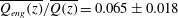 $\overline{Q_{eng}(z)}/\overline{Q(z)}=0.065\pm 0.018$
. We note that this should not be compared to values determined by calculations of the form presented by (4.9) since these, in effect, assume that the vertical velocity is independent of whether fluid at a given instant was engulfed or mixed plume fluid which we have shown is not the case (figure 6). Indeed, making a similar assumption with our data has a dramatic impact, approximately doubling the estimate of the engulfed volume flux. Figure 12 also shows that proportion of the volume flux consisting of engulfed fluid is lower when eddies are present (
$\overline{Q_{eng}(z)}/\overline{Q(z)}=0.065\pm 0.018$
. We note that this should not be compared to values determined by calculations of the form presented by (4.9) since these, in effect, assume that the vertical velocity is independent of whether fluid at a given instant was engulfed or mixed plume fluid which we have shown is not the case (figure 6). Indeed, making a similar assumption with our data has a dramatic impact, approximately doubling the estimate of the engulfed volume flux. Figure 12 also shows that proportion of the volume flux consisting of engulfed fluid is lower when eddies are present (
 $\overline{Q_{eng,e}(z)}/\overline{Q_{e}(z)}=0.039\pm 0.015$
) and increases when eddies are absent (
$\overline{Q_{eng,e}(z)}/\overline{Q_{e}(z)}=0.039\pm 0.015$
) and increases when eddies are absent (
 $\overline{Q_{eng,n}(z)}/\overline{Q_{n}(z)}=0.081\pm 0.024$
). This indicates that the large-scale coherent structures may be mixing much of the engulfed fluid, i.e. transforming engulfed fluid into mixed plume fluid and not just stirring fluid.
$\overline{Q_{eng,n}(z)}/\overline{Q_{n}(z)}=0.081\pm 0.024$
). This indicates that the large-scale coherent structures may be mixing much of the engulfed fluid, i.e. transforming engulfed fluid into mixed plume fluid and not just stirring fluid.
Our estimate of the vertical volume flux outside the plume is nearly 5 % of the total volume flux. Since we estimate the engulfed volume flux to be approximately 7 % of the total, almost all the vertical volume flux outside the plume must be engulfed. The fact that the engulfed flux is larger than the flux outside the plume is an alternative illustration that fluid must also be accelerated vertically during this engulfment, see also figure 6. This illustrates the significant role that engulfment plays within the process of turbulent entrainment by plumes.
4.3 The velocity field in plume coordinates

Figure 13. Vertical (solid lines) and horizontal (dashed lines) velocities averaged in the plume coordinate system,
 $r_{p}$
. The full time-averaged velocities,
$r_{p}$
. The full time-averaged velocities,
 $\overline{w_{p}}$
and
$\overline{w_{p}}$
and
 $\overline{u_{p}}$
, are marked in black; average velocities when eddies are present,
$\overline{u_{p}}$
, are marked in black; average velocities when eddies are present,
 $\overline{w_{(p,e)}}$
and
$\overline{w_{(p,e)}}$
and
 $\overline{u_{(p,e)}}$
, are marked in green; average velocities when no eddies are present,
$\overline{u_{(p,e)}}$
, are marked in green; average velocities when no eddies are present,
 $\overline{w_{(p,n)}}$
and
$\overline{w_{(p,n)}}$
and
 $\overline{u_{(p,n)}}$
, are marked in red. The data from three different plumes at 18 different heights exhibit a broad collapse indicating self-similarity. The vertical velocities outside the plume are significant near the plume edge and are, indeed, greater than the horizontal velocities at the same location. The dashed magenta curve is a Gaussian of variance equal to mean variance of the ensemble data (black curves).
$\overline{u_{(p,n)}}$
, are marked in red. The data from three different plumes at 18 different heights exhibit a broad collapse indicating self-similarity. The vertical velocities outside the plume are significant near the plume edge and are, indeed, greater than the horizontal velocities at the same location. The dashed magenta curve is a Gaussian of variance equal to mean variance of the ensemble data (black curves).

Figure 14. (a) The root mean square of the fluctuations in vertical (solid lines) and horizontal (dashed lines) velocities and (b)
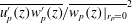 $\overline{u_{p}^{\prime }(z)w_{p}^{\prime }(z)}/\overline{w_{p}(z)|_{r_{p}=0}}^{2}$
averaged in the plume coordinate system,
$\overline{u_{p}^{\prime }(z)w_{p}^{\prime }(z)}/\overline{w_{p}(z)|_{r_{p}=0}}^{2}$
averaged in the plume coordinate system,
 $r_{p}$
. The vertical velocity fluctuations exhibit bi-modal peaks of approximately 25 %–30 % of the mean velocities at
$r_{p}$
. The vertical velocity fluctuations exhibit bi-modal peaks of approximately 25 %–30 % of the mean velocities at
 $r_{p}\approx \{-0.5R_{p},0.5R_{p}\}$
. The horizontal velocity fluctuations exhibit a broad peak around the centreline, the peak values are almost 15 % of the mean vertical velocities – this corresponds to the fluctuations being approximately three times larger than the maximum time-averaged horizontal velocities within the plume.
$r_{p}\approx \{-0.5R_{p},0.5R_{p}\}$
. The horizontal velocity fluctuations exhibit a broad peak around the centreline, the peak values are almost 15 % of the mean vertical velocities – this corresponds to the fluctuations being approximately three times larger than the maximum time-averaged horizontal velocities within the plume.
To provide further insights into the process of entrainment by plumes we examine the flow in a coordinate system which follows the plume as it meanders and fluctuates in width. At each time and height, we defined a local coordinate system in which the position
 $r_{p}=0(z,t)$
was the instantaneous mid-point of the edges from the scalar field at that height. We then record the velocities in a plume coordinate system
$r_{p}=0(z,t)$
was the instantaneous mid-point of the edges from the scalar field at that height. We then record the velocities in a plume coordinate system
 $r_{p}(z,t)$
, in which
$r_{p}(z,t)$
, in which
 $r_{p}(z,t)=-R_{p}(z,t)=E_{L}(z,t)$
,
$r_{p}(z,t)=-R_{p}(z,t)=E_{L}(z,t)$
,
 $r_{p}(z,t)=0(z,t)$
and
$r_{p}(z,t)=0(z,t)$
and
 $r_{p}(z,t)=R_{p}(z,t)=E_{R}(z,t)$
denote the instantaneous left-hand edge, mid-point and right-hand edge of the plume, respectively. The velocity data were then time averaged to obtain the average vertical velocity in this plume coordinate system, defined by
$r_{p}(z,t)=R_{p}(z,t)=E_{R}(z,t)$
denote the instantaneous left-hand edge, mid-point and right-hand edge of the plume, respectively. The velocity data were then time averaged to obtain the average vertical velocity in this plume coordinate system, defined by
 $$\begin{eqnarray}\overline{w_{p}}=\overline{w(r_{p},z)}=\frac{1}{T}\int _{0}^{T}w(r_{p},z,t)\,\text{d}t,\end{eqnarray}$$
and the equivalently defined horizontal velocity
 $\overline{u_{p}}$
. These data are plotted as the black curves in figure 13. The figure shows data from the three different plumes at 18 different heights and with the plume coordinate system calculated from both edge-detection algorithms (see § 2.2), as is also the case in figures 13–15. To our knowledge, this is the first time that velocity data for either jets or plumes have been conditionally averaged in this manner, cf. Wang & Law (Reference Wang and Law2002), Westerweel et al. (Reference Westerweel, Fukushima, Pedersen and Hunt2009) and Mistry et al. (Reference Mistry, Philip, Dawson and Marusic2016).
$\overline{u_{p}}$
. These data are plotted as the black curves in figure 13. The figure shows data from the three different plumes at 18 different heights and with the plume coordinate system calculated from both edge-detection algorithms (see § 2.2), as is also the case in figures 13–15. To our knowledge, this is the first time that velocity data for either jets or plumes have been conditionally averaged in this manner, cf. Wang & Law (Reference Wang and Law2002), Westerweel et al. (Reference Westerweel, Fukushima, Pedersen and Hunt2009) and Mistry et al. (Reference Mistry, Philip, Dawson and Marusic2016).
The average data collapse onto a single curve showing that the velocities are self-similar when viewed in plume coordinates. The average vertical velocities at the plume edge (black vertical lines at
 $\{-R_{p},R_{p}\}$
) are significant, and almost 20 % of the velocities on the centreline. Similar vertical velocities at the plume edge were also observed by the recent study of Burridge et al. (Reference Burridge, Partridge and Linden2016) in which visible coherent structures were tracked using a cross-correlation technique. These structures at the plume edge (found to be of width
$\{-R_{p},R_{p}\}$
) are significant, and almost 20 % of the velocities on the centreline. Similar vertical velocities at the plume edge were also observed by the recent study of Burridge et al. (Reference Burridge, Partridge and Linden2016) in which visible coherent structures were tracked using a cross-correlation technique. These structures at the plume edge (found to be of width
 ${\sim}0.4R_{p}$
) travelled at approximately 30 % of the centreline velocities, similar to the velocities just inside of the plume edge shown in figure 13.
${\sim}0.4R_{p}$
) travelled at approximately 30 % of the centreline velocities, similar to the velocities just inside of the plume edge shown in figure 13.
The root mean square of the velocity fluctuations in the plume coordinate are shown in figure 14(a). When observed in this frame of reference the mean profiles for the vertical velocity fluctuations exhibit bi-modal peaks of approximately 25 %–30 % of the mean velocities, somewhat larger than when observed in a fixed Eulerian coordinate (cf. figures 7
a or 10
a). This suggests that the spatial intermittency (the meandering and fluctuations in width) of the plume must, to some extent, mask the scale of the turbulent velocity fluctuations. The same effects are not evident in the quantities of the form
 $\overline{u_{p}^{\prime }(z)w_{p}^{\prime }(z)}$
(cf. figures 7
b and 10
b) – it is not obvious why this should be the case.
$\overline{u_{p}^{\prime }(z)w_{p}^{\prime }(z)}$
(cf. figures 7
b and 10
b) – it is not obvious why this should be the case.
The locations of the peaks in the vertical velocity fluctuations, at
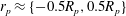 $r_{p}\approx \{-0.5R_{p},0.5R_{p}\}$
, roughly correspond to the locations at which the radial velocities in the plume are zero. The radial velocity fluctuations exhibit a single broad peak about the centreline, with peak values that are almost 15 % of the mean vertical velocities. This value corresponds to the fluctuations in horizontal velocities being approximately 300 % of the maximum time-averaged horizontal velocities within the plume. Thus the mean horizontal velocities established by the process of entrainment are small compared with the fluctuating horizontal velocities within the falling, swirling coherent structures which form (with some complex and chaotic orientation) within the plume.
$r_{p}\approx \{-0.5R_{p},0.5R_{p}\}$
, roughly correspond to the locations at which the radial velocities in the plume are zero. The radial velocity fluctuations exhibit a single broad peak about the centreline, with peak values that are almost 15 % of the mean vertical velocities. This value corresponds to the fluctuations in horizontal velocities being approximately 300 % of the maximum time-averaged horizontal velocities within the plume. Thus the mean horizontal velocities established by the process of entrainment are small compared with the fluctuating horizontal velocities within the falling, swirling coherent structures which form (with some complex and chaotic orientation) within the plume.
4.3.1 Plume properties when eddies are present and absent
We extend our examination of the velocity fields in the plume coordinate and compare how they vary from the mean depending on whether one might reasonably expect a large-scale coherent structure (eddy) to be locally present or absent at a given height. We recalculate the statistics in § 4.3 conditioned on the presence or absence of a large-scale eddy in a similar manner to that described for the fixed Eulerian coordinate in § 4.2.1. For example, we calculate the vertical velocity in the plume coordinate in the presence of an eddy as
 $$\begin{eqnarray}\overline{w_{(p,e)}}=\overline{w_{(p,e)}(r_{p},z)}=\frac{1}{T_{e}}\int _{0}^{T_{e}}H_{e}(r_{p},z,t)w(r_{p},z,t)\,\text{d}t.\end{eqnarray}$$
The data for the velocities when eddies are present (green curves) and absent (red curves) are plotted in figure 13. As is the case for the ensemble data (black curves), these conditional data collapse for each state, showing that the plume statistics are self-similar in all three states when viewed in the plume coordinate
 $r_{p}$
. The data in figure 13 are normalised by the ensemble mean centreline velocity. It is noteworthy that the mean velocity in the middle of the plume, i.e.
$r_{p}$
. The data in figure 13 are normalised by the ensemble mean centreline velocity. It is noteworthy that the mean velocity in the middle of the plume, i.e.
 $r_{p}=0$
, systematically varied by a few per cent between the three states. Larger vertical velocities were observed in the middle of the plumes when eddies were locally absent; however, in the fixed Eulerian coordinate larger vertical velocities were observed on the centreline,
$r_{p}=0$
, systematically varied by a few per cent between the three states. Larger vertical velocities were observed in the middle of the plumes when eddies were locally absent; however, in the fixed Eulerian coordinate larger vertical velocities were observed on the centreline,
 $r=0$
, when eddies were present. This difference highlights the sensitivity of the observations to the choice of reference frame.
$r=0$
, when eddies were present. This difference highlights the sensitivity of the observations to the choice of reference frame.
The velocity profiles plotted in figure 13 show large vertical velocities outside the plume (up to 40 % of the maximum velocities) when large-scale coherent structures are absent. Conversely, when eddies are present there is almost zero vertical velocity at and beyond the plume edge. Such findings are in agreement with, and provide an alternative illustration of, our results for the vertical transport outside the plume presented in § 4.2.1. Moreover, the velocity data differ significantly between the three states. For example, when an eddy is locally present, the vertical velocities at the plume edge are smaller by about a factor of four compared to the mean, and by approximately a factor of ten compared to when an eddy is absent. Horizontal velocities, on the other hand, are larger by about a factor of four when an eddy is absent compared to when present, indicating that ambient fluid is drawn towards the plume at height between eddies.
Figure 14 includes the velocity fluctuations and quantities of the form
 $\overline{u_{p}^{\prime }(z)w_{p}^{\prime }(z)}$
, conditioned on the presence and absence of eddies. When viewed in this coordinate the data from inside the plume are, broadly similar for each of the three states, which is in contrast to the measurements of velocity fluctuations and Reynolds stresses in the Eulerian coordinate (cf. figure 10). This may indicate that the velocity field within the plume scales more appropriately on a radial coordinate based on the local instantaneous width of the plume (our plume coordinate) than on the local time-averaged width (as is the case for the Eulerian coordinate), confirming that variations in plume width are correlated with the internal flow structures. Outside the plume the data for the velocity fluctuations (figure 14
a) show variations from the mean when eddies are both present or absent. However, the data for
$\overline{u_{p}^{\prime }(z)w_{p}^{\prime }(z)}$
, conditioned on the presence and absence of eddies. When viewed in this coordinate the data from inside the plume are, broadly similar for each of the three states, which is in contrast to the measurements of velocity fluctuations and Reynolds stresses in the Eulerian coordinate (cf. figure 10). This may indicate that the velocity field within the plume scales more appropriately on a radial coordinate based on the local instantaneous width of the plume (our plume coordinate) than on the local time-averaged width (as is the case for the Eulerian coordinate), confirming that variations in plume width are correlated with the internal flow structures. Outside the plume the data for the velocity fluctuations (figure 14
a) show variations from the mean when eddies are both present or absent. However, the data for
 $\overline{u_{p}^{\prime }(z)w_{p}^{\prime }(z)}$
, figure 14(b), show a significant variation from the mean only when eddies are absent. Both in the mean and when eddies are present,
$\overline{u_{p}^{\prime }(z)w_{p}^{\prime }(z)}$
, figure 14(b), show a significant variation from the mean only when eddies are absent. Both in the mean and when eddies are present,
 $\overline{u_{p}^{\prime }(z)w_{p}^{\prime }(z)}$
is positive within the plume and zero outside which implies that the unsteady transport of vertical momentum is radially outwards. In the case when eddies are absent,
$\overline{u_{p}^{\prime }(z)w_{p}^{\prime }(z)}$
is positive within the plume and zero outside which implies that the unsteady transport of vertical momentum is radially outwards. In the case when eddies are absent,
 $\overline{u_{p}^{\prime }(z)w_{p}^{\prime }(z)}$
is positive within the plume and negative outside suggesting that at heights between eddies the unsteady transport of vertical momentum is radially inwards. Such a finding is supportive of our view that vertical momentum is imparted on ambient fluid at heights between eddies, before this ambient fluid is engulfed.
$\overline{u_{p}^{\prime }(z)w_{p}^{\prime }(z)}$
is positive within the plume and negative outside suggesting that at heights between eddies the unsteady transport of vertical momentum is radially inwards. Such a finding is supportive of our view that vertical momentum is imparted on ambient fluid at heights between eddies, before this ambient fluid is engulfed.

Figure 15. The angle to the horizontal of the velocity vectors averaged in the plume coordinate system,
 $r_{p}$
. The angles from the full time averages are marked in black, those averaged only when eddies are present are marked in green and those when no eddies are present are marked in red. Steep radial gradients in the angles are only observed at the plume edge when eddies are present.
$r_{p}$
. The angles from the full time averages are marked in black, those averaged only when eddies are present are marked in green and those when no eddies are present are marked in red. Steep radial gradients in the angles are only observed at the plume edge when eddies are present.
The relative magnitude of the vertical and horizontal velocities in the plume are illustrated by calculating the angle formed by the local velocity vectors to the horizontal. The data shown in figure 15 marked by the black curves illustrate the ensemble mean and show that, at the plume edge, the average vertical velocities are large compared with the horizontal velocities (the angle being approximately
 $70^{\circ }$
). The mean the vertical and horizontal velocities are only of equal magnitude (and the angle close to
$70^{\circ }$
). The mean the vertical and horizontal velocities are only of equal magnitude (and the angle close to
 $45^{\circ }$
) at distances of approximately
$45^{\circ }$
) at distances of approximately
 $\pm 1.2R_{p}$
, i.e. some distance outside the plume. Differences in the velocity field between eddy present and absent events are also clearly highlighted in figure 15. When an eddy is present (green curves), the angle increases rapidly from close to horizontal (
$\pm 1.2R_{p}$
, i.e. some distance outside the plume. Differences in the velocity field between eddy present and absent events are also clearly highlighted in figure 15. When an eddy is present (green curves), the angle increases rapidly from close to horizontal (
 $0^{\circ }$
) just outside the plume edge to being close to vertical (
$0^{\circ }$
) just outside the plume edge to being close to vertical (
 ${\sim}90^{\circ }$
) just within the plume edge. When eddies are absent vertical and horizontal velocities are only of equal magnitude at distances significantly outside the plume, of approximately
${\sim}90^{\circ }$
) just within the plume edge. When eddies are absent vertical and horizontal velocities are only of equal magnitude at distances significantly outside the plume, of approximately
 $\pm 1.7R_{p}$
. These findings support the suggestion (§ 4.2) that prior to being engulfed or entrained, ambient fluid already has a significant component of vertical velocity and thereby momentum.
$\pm 1.7R_{p}$
. These findings support the suggestion (§ 4.2) that prior to being engulfed or entrained, ambient fluid already has a significant component of vertical velocity and thereby momentum.

Figure 16. Time-averaged views of a turbulent plume: (a) all observations, (b) observations when eddies are present, (c) when eddies are absent. The black lines mark the time-averaged position of the edge of the plume scalar field in each of the three states. The (blue) arrows mark the magnitude and direction of the measured velocity vectors (ensemble averaged over the 18 heights shown in figure 13). The axis are marked in arbitrary units.
The data for the horizontal and vertical velocities in the plume coordinate
 $r_{p}$
(figure 13) and the time-averaged position of the plume edge
$r_{p}$
(figure 13) and the time-averaged position of the plume edge
 $\overline{R_{p}}$
(figure 3) allow us to reconstruct the velocity field induced by and within a plume, relative to the scalar edge of the plume. These data are plotted in figure 16(a) and we note that the data from a simple Eulerian view of the plume would look notionally identical. The figure shows that ambient fluid outside the scalar edge is drawn towards the plume, by the process of turbulent entrainment, but that as part of this process significant vertical velocity is induced within the ambient fluid before reaching the edge of the plume. The role that coherent structures play in this process is indicated by comparing equivalent reconstructions of the velocity field using data from observations when one can expect large-scale eddies to be present or absent, figures 16(b) and 16(c), respectively. When eddies are present, the velocities within the (relatively wide) plume are almost entirely vertical and the flow outside predominately horizontal. Conversely, when eddies are absent the velocities within the (relatively thin) plume show a marked component of horizontal velocity well within the scalar edge and, crucially, ambient fluid far outside the scalar edges exhibits a significant component of vertical velocity and therefore momentum, before it is entrained into the plume.
$\overline{R_{p}}$
(figure 3) allow us to reconstruct the velocity field induced by and within a plume, relative to the scalar edge of the plume. These data are plotted in figure 16(a) and we note that the data from a simple Eulerian view of the plume would look notionally identical. The figure shows that ambient fluid outside the scalar edge is drawn towards the plume, by the process of turbulent entrainment, but that as part of this process significant vertical velocity is induced within the ambient fluid before reaching the edge of the plume. The role that coherent structures play in this process is indicated by comparing equivalent reconstructions of the velocity field using data from observations when one can expect large-scale eddies to be present or absent, figures 16(b) and 16(c), respectively. When eddies are present, the velocities within the (relatively wide) plume are almost entirely vertical and the flow outside predominately horizontal. Conversely, when eddies are absent the velocities within the (relatively thin) plume show a marked component of horizontal velocity well within the scalar edge and, crucially, ambient fluid far outside the scalar edges exhibits a significant component of vertical velocity and therefore momentum, before it is entrained into the plume.
Physically, a plume is never in a state of having either eddies present or absent throughout its height; quite the contrary is typical. At any instant, a plume exhibits an alternating pattern of eddies being locally present and absent throughout its height (see, for example, the images in figure 1). Figure 16(b,c) illustrates that between the large-scale coherent structures, vertical momentum is imparted (presumably by pressure gradients) to pockets of ambient fluid that are, in a relative sense, quite close to the plume centreline. The vertical momentum of these pockets of ambient fluid enable them to be engulfed into the plume more easily, providing a source for the volume flux of engulfed fluid identified in our measurements (§ 4.2.2 and figure 12).
These findings suggest that ambient fluid is being accelerated vertically before reaching the plume edge. This acceleration of ambient fluid cannot be as a result of viscous effects at the plume edge and must result from relatively long-range pressure gradients, as has been shown for planar jets (Taveira & da Silva Reference Taveira and da Silva2013; Terashima et al. Reference Terashima, Sakai, Nagata, Ito, Onishi and Shouji2016) and (shear free) oscillating grids (Holzner et al. Reference Holzner, Lüthi, Tsinober and Kinzelbach2009). Thus turbulent entrainment must, at the initial engulfment stage, be driven by these pressure gradients and not by viscous effects at the plume edge (cf. Westerweel et al. Reference Westerweel, Fukushima, Pedersen and Hunt2009). Such a view of entrainment is entirely consistent with the view of entrainment expressed by Philip et al. (Reference Philip, Meneveau, de Silva and Marusic2014) for turbulent boundary layers and by Mistry et al. (Reference Mistry, Philip, Dawson and Marusic2016) for turbulent (non-buoyant) jets.
4.4 The relative widths of the scalar and velocity fields
Our findings, for example the radial distribution of vertical velocity (figure 13), show that there is a significant vertical flow outside the plume envelope (defined for high Péclet number plumes by the loci of the scalar edges). If the average scalar concentrations follow the same radial distribution as the average vertical velocity then, since we observe vertical velocities beyond the edge of the scalar field, one would expect the characteristic width of velocity distribution to be wider than that of the scalar. However, figure 17 shows that the time-averaged plume widths determined by the edges of the scalar field,
 $\overline{R_{p}}$
, and the (top-hat) plume width based on the velocity field,
$\overline{R_{p}}$
, and the (top-hat) plume width based on the velocity field,
 $\overline{R}$
, are approximately equal, i.e.
$\overline{R}$
, are approximately equal, i.e.
 $\unicode[STIX]{x1D706}_{1}\equiv \overline{R_{p}}/\overline{R}=0.98\pm 0.04\approx 1$
. This can only be consistent with our observation of significant vertical velocities beyond the scalar edge of the plume if the velocity and scalar concentrations follow different radial distributions, and the scalar distribution is closer to a uniform ‘well-mixed’ distribution within the mixed plume fluid than the velocity distribution.
$\unicode[STIX]{x1D706}_{1}\equiv \overline{R_{p}}/\overline{R}=0.98\pm 0.04\approx 1$
. This can only be consistent with our observation of significant vertical velocities beyond the scalar edge of the plume if the velocity and scalar concentrations follow different radial distributions, and the scalar distribution is closer to a uniform ‘well-mixed’ distribution within the mixed plume fluid than the velocity distribution.

Figure 17. The variation of
 $\unicode[STIX]{x1D706}_{1}=\overline{R_{p}}/\overline{R}$
(solid lines) and
$\unicode[STIX]{x1D706}_{1}=\overline{R_{p}}/\overline{R}$
(solid lines) and
 $\unicode[STIX]{x1D706}_{2}=\tilde{R}_{g}/\tilde{R}_{w}$
(dotted lines) with the vertical coordinate,
$\unicode[STIX]{x1D706}_{2}=\tilde{R}_{g}/\tilde{R}_{w}$
(dotted lines) with the vertical coordinate,
 $z/r_{0}$
. The mean values are plotted (thin lines) and given in the legend.
$z/r_{0}$
. The mean values are plotted (thin lines) and given in the legend.
To test such a hypothesis, one can then conceive a simplified model, in which the region between the scalar edges consists of fluid with only two scalar concentrations of, say, zero (i.e. engulfed unmixed fluid) or unity (mixed plume fluid), respectively. We can examine the results of such an idealised model by taking our experimental data for
 $H_{eng}$
and
$H_{eng}$
and
 $H_{mix}$
(see § 4.2.2).
$H_{mix}$
(see § 4.2.2).
When time averaged in an Eulerian frame this idealised (uniform) distribution of mixed plume fluid (not shown) exhibits a good approximation to a Gaussian profile (just as is observed for the velocity, figure 2). This shows that spatial (meandering) and temporal (fluctuating) intermittency are sufficient to result in a Gaussian distribution being observed for the buoyancy scalar, in an Eulerian frame, even in the limiting case that the scalar concentration within mixed plume fluid is uniform at a given height at all times. Given that observations in an Eulerian frame result in approximate Gaussian distributions for both the velocity and the model scalar distribution, we can then define the characteristic width of the scalar distribution of mixed plume fluid
 $\tilde{R}_{g}$
from this idealised model based on the e-folding width, in a manner entirely equivalent to
$\tilde{R}_{g}$
from this idealised model based on the e-folding width, in a manner entirely equivalent to
 $\tilde{R}_{w}$
for the velocity (see § 3). Evaluating these widths enables an estimate
$\tilde{R}_{w}$
for the velocity (see § 3). Evaluating these widths enables an estimate
 $\unicode[STIX]{x1D706}_{2}\equiv \tilde{R}_{g}/\tilde{R}_{w}$
of the relative widths of the velocity field and the scalar field from our idealised model (assuming mixed plume fluid is of a single concentration at any height).
$\unicode[STIX]{x1D706}_{2}\equiv \tilde{R}_{g}/\tilde{R}_{w}$
of the relative widths of the velocity field and the scalar field from our idealised model (assuming mixed plume fluid is of a single concentration at any height).
The data for
 $\unicode[STIX]{x1D706}_{2}$
are shown in figure 17, for which
$\unicode[STIX]{x1D706}_{2}$
are shown in figure 17, for which
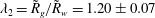 $\unicode[STIX]{x1D706}_{2}=\tilde{R}_{g}/\tilde{R}_{w}=1.20\pm 0.07$
. Hence, our measurements of the velocity and scalar field in the plume suggest that, even in the limiting case that mixed plume fluid is of a single concentration, observations made in an Eulerian frame would follow a Gaussian distribution that is approximately 20 % wider for the scalar than that observed for the velocity. Hence, measurements made in a fixed Eulerian frame, as has typically been the case, would imply a ratio of characteristic widths
$\unicode[STIX]{x1D706}_{2}=\tilde{R}_{g}/\tilde{R}_{w}=1.20\pm 0.07$
. Hence, our measurements of the velocity and scalar field in the plume suggest that, even in the limiting case that mixed plume fluid is of a single concentration, observations made in an Eulerian frame would follow a Gaussian distribution that is approximately 20 % wider for the scalar than that observed for the velocity. Hence, measurements made in a fixed Eulerian frame, as has typically been the case, would imply a ratio of characteristic widths
 $\unicode[STIX]{x1D706}$
, in the range
$\unicode[STIX]{x1D706}$
, in the range
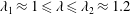 $\unicode[STIX]{x1D706}_{1}\approx 1\leqslant \unicode[STIX]{x1D706}\leqslant \unicode[STIX]{x1D706}_{2}\approx 1.2$
, the exact value of which would depend on just how close to being of uniform concentration the mixed plume fluid actually is. It is somewhat of a pity that the literature provides little clarity as to which value within this range is the most appropriate value for
$\unicode[STIX]{x1D706}_{1}\approx 1\leqslant \unicode[STIX]{x1D706}\leqslant \unicode[STIX]{x1D706}_{2}\approx 1.2$
, the exact value of which would depend on just how close to being of uniform concentration the mixed plume fluid actually is. It is somewhat of a pity that the literature provides little clarity as to which value within this range is the most appropriate value for
 $\unicode[STIX]{x1D706}$
. For example, Papantoniou & List (Reference Papantoniou and List1989), Panchapakesan & Lumley (Reference Panchapakesan and Lumley1993), Ezzamel et al. (Reference Ezzamel, Salizzoni and Hunt2015) all report values of
$\unicode[STIX]{x1D706}$
. For example, Papantoniou & List (Reference Papantoniou and List1989), Panchapakesan & Lumley (Reference Panchapakesan and Lumley1993), Ezzamel et al. (Reference Ezzamel, Salizzoni and Hunt2015) all report values of
 $\unicode[STIX]{x1D706}\approx 1.2$
, while Wang & Law (Reference Wang and Law2002), Craske & van Reeuwijk (Reference Craske and van Reeuwijk2016) report values of
$\unicode[STIX]{x1D706}\approx 1.2$
, while Wang & Law (Reference Wang and Law2002), Craske & van Reeuwijk (Reference Craske and van Reeuwijk2016) report values of
 $\unicode[STIX]{x1D706}\approx 1.0$
.
$\unicode[STIX]{x1D706}\approx 1.0$
.
However, what is clear from our data and the above analysis, is that distinctly different mixing and transport mechanisms produce the distributions of scalar quantities (e.g. buoyancy, dyes, contaminants, etc.) and velocities (directional momentum) within the plume. These different mechanisms result in different physical distributions for the velocity and buoyancy in plumes and it is only a result of the significant role of spatial and temporal intermittency in determining the location and width of the plume which statistically results in Gaussian distributions being observed for both quantities – such observations only being evident in a fixed Eulerian view of the plume. Moreover, the frame of reference in which such measurements are made (e.g. an Eulerian coordinate fixed in space or, for example, a spatial coordinate based on the plume width) entirely alters whether one concludes that the velocity or scalar follow a wider distribution. Consequently, this implies that a description of the ratio of the characteristic widths of the distribution of the velocity and scalar fields observed in a fixed Eulerian coordinate as being representative of the ‘turbulent Prandtl number’ in a plume are misleading. For example, van Reeuwijk et al. (Reference van Reeuwijk, Salizzoni, Hunt and Craske2016) show that this ratio is indeed indicative of the turbulent Prandtl number in pure momentum jets but that this is not the case for buoyant plumes.
Our measurements of the velocity distribution in the plume coordinate, i.e. in the absence of the influence of intermittency (meandering and fluctuating in width), exhibit a reasonable fit to a Gaussian distribution, the dashed magenta curve in figure 13. For an unbounded quantity of fixed variance a Gaussian distribution maximises the differential entropy, where the differential entropy is defined by
 $-\!\int f(r)\ln (f(r))\,\text{d}r$
, with
$-\!\int f(r)\ln (f(r))\,\text{d}r$
, with
 $f(r)$
being the radial distribution of the vertical velocity or the buoyancy scalar. Consequently, the velocities observed in the plume coordinate indicate that the mixing of momentum across the plume results in a distribution for which the differential entropy is close to maximal. Furthermore, the velocity distribution in the plume coordinate exhibiting properties close to that of a maximum differential entropy distribution for an unbounded quantity, indicates that the mixing must be controlled by long-range forces that are not inhibited by the TNTI, i.e. the mixing of momentum must be controlled by the pressure field. With this in mind it would perhaps provide some insight into the physics controlling the process of the scalar mixing across the plume to determine an appropriate value for the ratio of the widths
$f(r)$
being the radial distribution of the vertical velocity or the buoyancy scalar. Consequently, the velocities observed in the plume coordinate indicate that the mixing of momentum across the plume results in a distribution for which the differential entropy is close to maximal. Furthermore, the velocity distribution in the plume coordinate exhibiting properties close to that of a maximum differential entropy distribution for an unbounded quantity, indicates that the mixing must be controlled by long-range forces that are not inhibited by the TNTI, i.e. the mixing of momentum must be controlled by the pressure field. With this in mind it would perhaps provide some insight into the physics controlling the process of the scalar mixing across the plume to determine an appropriate value for the ratio of the widths
 $\unicode[STIX]{x1D706}$
. For example, our above analysis indicates that a value of
$\unicode[STIX]{x1D706}$
. For example, our above analysis indicates that a value of
 $\unicode[STIX]{x1D706}\approx 1.2$
indicates that the scalar is (at all times) relatively well mixed, i.e. close to a uniform distribution, within mixed plume fluid. The uniform distribution is the maximum differential entropy distribution for a quantity which is strictly bounded in a finite domain. Hence, if
$\unicode[STIX]{x1D706}\approx 1.2$
indicates that the scalar is (at all times) relatively well mixed, i.e. close to a uniform distribution, within mixed plume fluid. The uniform distribution is the maximum differential entropy distribution for a quantity which is strictly bounded in a finite domain. Hence, if
 $\unicode[STIX]{x1D706}\approx 1.2$
then one could conclude that both the mixing of both momentum and scalars across high Péclet number turbulent pure plumes result in distributions that are, at least close to, distributions for which the differential entropy is maximal. In the case of the mixing of momentum long-range pressure forces enable the mixing to be uninhibited by the plume edges, while the scalar mixing is strictly bounded by the edges of the high Péclet number plume.
$\unicode[STIX]{x1D706}\approx 1.2$
then one could conclude that both the mixing of both momentum and scalars across high Péclet number turbulent pure plumes result in distributions that are, at least close to, distributions for which the differential entropy is maximal. In the case of the mixing of momentum long-range pressure forces enable the mixing to be uninhibited by the plume edges, while the scalar mixing is strictly bounded by the edges of the high Péclet number plume.
5 Conclusions
Simultaneous measurements of the velocity field and the scalar edge of a plume have shown that significant vertical velocities exist outside the plume. Velocities beyond the plume edge cannot be induced by viscous effects at the plume edge and must be induced by relatively long-range pressure gradients (consistent with findings for other entraining flows, e.g. Holzner et al. Reference Holzner, Lüthi, Tsinober and Kinzelbach2009; Taveira & da Silva Reference Taveira and da Silva2013; Terashima et al. Reference Terashima, Sakai, Nagata, Ito, Onishi and Shouji2016). The vertical transport outside the plume, i.e. within ambient fluid, is in the mean approximately 5 % of the total vertical transport, with this rising to almost 14 % at heights between eddies. These (and others of our findings) indicate that significant vertical momentum is imparted to ambient fluid, at least, at heights between eddies before this ambient fluid comes into contact with the edge (turbulent/non-turbulent interface) of the plume.
Our measurements show that, in the mean, the flux of engulfed fluid (i.e. unmixed fluid within the plume envelope) is
 $6.5\,\%\pm 2\,\%$
of the total vertical transport. We can account for the suggestion that the flux of engulfed fluid is greater than the transport outside the plume since we have shown that engulfed fluid at a given radial location travels faster than ambient at the same location, i.e. fluid must be accelerated vertically as it is engulfed. Even with this in mind, we are still able to conclude that our findings show that almost all the ambient fluid moving vertically outside the plume must be engulfed into the plume. It is not trivial to relate findings regarding the vertical fluxes of ambient or engulfed fluid to statements of the bulk entrainment rate (
$6.5\,\%\pm 2\,\%$
of the total vertical transport. We can account for the suggestion that the flux of engulfed fluid is greater than the transport outside the plume since we have shown that engulfed fluid at a given radial location travels faster than ambient at the same location, i.e. fluid must be accelerated vertically as it is engulfed. Even with this in mind, we are still able to conclude that our findings show that almost all the ambient fluid moving vertically outside the plume must be engulfed into the plume. It is not trivial to relate findings regarding the vertical fluxes of ambient or engulfed fluid to statements of the bulk entrainment rate (
 $\text{d}\overline{Q}/\text{d}z$
), since to do so requires knowledge of the length and time scales associated with the processes of engulfment and ultimately mixing. However, it is something that we hope is addressed in the near future.
$\text{d}\overline{Q}/\text{d}z$
), since to do so requires knowledge of the length and time scales associated with the processes of engulfment and ultimately mixing. However, it is something that we hope is addressed in the near future.
Examining our measurements when we expect large-scale coherent structures (eddies) to be locally either present or absent has highlighted substantial differences in the velocity field in the two cases, and we conclude that the passage of large-scale eddies at the plume edge drives pockets of ambient fluid at significant vertical velocities. The vertical momentum induced within these pockets of ambient fluid enables it to be engulfed within the plume. We conclude that the engulfment of ambient fluid by large-scale eddies at the plume edge constitutes a significant part of the process of turbulent entrainment by plumes.
We have shown that observing significant vertical velocities outside the scalar edge of the plume should not be taken to imply that the velocity field is wider than the scalar field. Indeed, we show that different mechanisms drive the mixing, and thereby distributions, of momentum (velocities) and scalars. Through observations following the meandering and fluctuations in the plume, we remove the effects of spatial intermittency. By utilising our plume coordinate, we show that it is only as a result of spatial and temporal intermittency that a Gaussian distribution is observed for the scalar but that a distribution close to a Gaussian is still observed for the velocity. We conclude that the mixing of momentum (velocity) across the plume results in a distribution for which the differential entropy is, at least, close to maximal when the mixing is not bounded by the TNTI of the plume, indicating that the mixing of momentum must be controlled by the pressure field.
Furthermore, our measurements of the scalar edges are consistent with observations in the Eulerian frame for the relative width of the distributions of scalars and velocities in the range
 $1.0\leqslant \unicode[STIX]{x1D706}\leqslant 1.2$
. Some previous studies find that
$1.0\leqslant \unicode[STIX]{x1D706}\leqslant 1.2$
. Some previous studies find that
 $\unicode[STIX]{x1D706}\approx 1.2$
(e.g. Ezzamel et al.
Reference Ezzamel, Salizzoni and Hunt2015). We show that such a value of
$\unicode[STIX]{x1D706}\approx 1.2$
(e.g. Ezzamel et al.
Reference Ezzamel, Salizzoni and Hunt2015). We show that such a value of
 $\unicode[STIX]{x1D706}$
suggests that the scalar concentration is approximately uniformly distributed within all of the mixed plume fluid at a given height. This in turn indicates that the scalar mixing across the plume results in a distribution for which the differential entropy is, at least, close to maximal but the mixing is strictly bounded by the scalar edge, and hence the TNTI for high Péclet numbers – the scalar mixing can be expected to be bounded since the process is ultimately controlled by diffusion. We, therefore, hope that a robust dataset for truly high-Péclet number plumes, that provides measurements of the full velocity and scalar fields might finally determine whether
$\unicode[STIX]{x1D706}$
suggests that the scalar concentration is approximately uniformly distributed within all of the mixed plume fluid at a given height. This in turn indicates that the scalar mixing across the plume results in a distribution for which the differential entropy is, at least, close to maximal but the mixing is strictly bounded by the scalar edge, and hence the TNTI for high Péclet numbers – the scalar mixing can be expected to be bounded since the process is ultimately controlled by diffusion. We, therefore, hope that a robust dataset for truly high-Péclet number plumes, that provides measurements of the full velocity and scalar fields might finally determine whether
 $\unicode[STIX]{x1D706}\approx 1.2$
(Papantoniou & List Reference Papantoniou and List1989; Panchapakesan & Lumley Reference Panchapakesan and Lumley1993; Ezzamel et al.
Reference Ezzamel, Salizzoni and Hunt2015) or
$\unicode[STIX]{x1D706}\approx 1.2$
(Papantoniou & List Reference Papantoniou and List1989; Panchapakesan & Lumley Reference Panchapakesan and Lumley1993; Ezzamel et al.
Reference Ezzamel, Salizzoni and Hunt2015) or
 $\unicode[STIX]{x1D706}\approx 1.0$
(Wang & Law Reference Wang and Law2002; Craske & van Reeuwijk Reference Craske and van Reeuwijk2016) since obtaining a consensus would enable further insights into the mixing processes in plumes.
$\unicode[STIX]{x1D706}\approx 1.0$
(Wang & Law Reference Wang and Law2002; Craske & van Reeuwijk Reference Craske and van Reeuwijk2016) since obtaining a consensus would enable further insights into the mixing processes in plumes.
Finally, we conclude that turbulent pure plumes provide a canonical high-Péclet number free shear flow which can be relatively easily reproduced in laboratories around the world. Future studies of this flow could further illuminate the role of coherent structures and/or the role of buoyancy on the mixing of momentum and scalars in turbulent flows. Such studies are to be encouraged.
Acknowledgements
The authors gratefully acknowledge the skills and expertise provided by the technical staff of the G. K. Batchelor laboratory. H.C.B. acknowledges insightful conversations with Mr T. David regarding maximal entropy distributions. This work was supported, in part, by the Leverhulme Trust Research Programme Grant RP2013-SL-008, the EPSRC Programme Grant EP/K034529/1, the Gulf of Mexico Research Institute and by iCASE awards from NERC and the UK Met Office (RG82562) and EPSRC and Arup (RG83017).


