3.1. Set-up

The experiments are carried out in a water tank whose cross-section is $0.25\,{\rm m}\times 0.25\,{\rm m}$. The tank is filled with distilled water up to height 0.6 m. A simplified sketch of the experimental set-up is presented in figure 3. The cylinder characteristics are detailed in table 1. Tank temperature is kept at 20 $^\circ$C in order to keep constant water density, viscosity and refractive index.

Figure 3. Sketch of the experimental set-up.

Although the phenomena examined here are independent from the initial conditions, as shown by Toupoint et al. (Reference Toupoint, Ern and Roig2019) and Ern et al. (Reference Ern, Mougel, Cazin, Lorite-Díez and Bourguet2020), the limited measurement volume requires a robust procedure for cylinder release. In that sense, an automatic device is used to ensure a repeatable and accurate drop of the cylinders. The device consists of two arrays of pins aligned in two perpendicular planes. The horizontal array of pins holds the cylinder below the free surface to avoid the presence of bubbles on the cylinder. The vertical array, which is controlled pneumatically, can be translated to carefully push and release the cylinder at the top of the tank.

A $527$ nm, $2\times 60\,{\rm mJ}$-per-pulse laser from Photonics Industries (ref. DM60-527-DH) is used to illuminate the seeding particles and the slightly fluorescent cylinder within the measurement volume. In order to light a delimited 3-D volume in the middle of the tank, an optical device (LaVision GmbH Volume Optics Module) expands the collimated laser beam. The sharp boundaries of this volume are delimited by knife-edge filters (see figure 3). A mirror is placed on the other side of the tank to increase the illumination in the volume. This double-pass illumination system increases the efficiency of the illumination by approximately $50\,\%$ (Scarano Reference Scarano2012).

The images are captured by four high-speed VEO640 Phantom cameras (equipped with 200 mm F/11 Nikon lenses) placed on a bench, at 100 cm from the frontal face of the tank. The cameras are set in a square-shaped arrangement; the distance between consecutive camera lenses is 67 cm. All the cameras are tilted by approximately 20$^{\circ }$ horizontally and vertically, towards the experiment. Respecting the Scheimpflug conditions, the lines of sight of the cameras are directed towards the centre of the illuminated volume. The emission peak of the seeding particles is located at approximately $568$ nm. To avoid reflections from the laser beam on the cylinder, the camera lenses are equipped with optical high-pass filters (540 nm).

The fluorescent seeding particles are polyamide covered with rhodamine B; their diameter is close to 22 $\mathrm {\mu }$m, and their density is $\rho _p \approx 1030\,{\rm kg}\,{\rm m}^{-3}$. For a typical experiment, the solute particles are introduced in the tank at several heights and then mixed to ensure their homogeneous distribution. The experiment is started 20 min after that. Following this procedure, the particle density, expressed in p.p.p. for particles per pixel (see Scarano Reference Scarano2012), ranges from $0.02$ to $0.025$ p.p.p.

The coordinate system $(X,Y,Z)$, related to the experimental set-up, is defined as shown in figures 1 and 3. The illuminated measurement volume has been defined by a 3-D calibration procedure detailed in § A.1. It has size $({\Delta}X_{v},\;{\Delta}Y_{v},\;{\Delta}Z_{v})=(132,\;86,\;35)$ mm, corresponding typically to $13d\unicode{x2013}35d$ in the horizontal direction and $48d\unicode{x2013}130d$ in the vertical one. The volume is located at mid-height of the tank, at distance 350 mm from the free surface; this location ensures that the permanent behaviour of the falling cylinder is reached, and also avoids any influence from the bottom wall. As indicated by previous measurements (Ern et al. Reference Ern, Mougel, Cazin, Lorite-Díez and Bourguet2020), the vertical extent of the present measurement volume, $Y_v$, is long enough to capture several periods of body oscillation, in most cases. The $X_v$ extent has been chosen to capture fully the longest cylinder, i.e. $L=110$ mm. The choice of $Z_v$ is a compromise between the typical width of cylinder wakes and the intensity of the seeding particles illumination.

The seeding particles located between the measurement volume and the front wall of the tank cause turbidity. Turbidity effect is actually small, but to further reduce it, the measurement volume is placed closer to the tank front wall. It has been verified that the distance from the wall remains sufficient to avoid any spurious interaction with the falling cylinder; the distance between the body and the wall is larger than 10$d$ even in the worst case.

3.2. Capture of fluid and body motions

The Shake-The-Box (STB) method is employed to capture the spatio-temporal evolution of the 3-D flow surrounding the cylinder, while the body dynamics is determined via tomographic reconstruction.

The STB method relies on a particle tracking algorithm that consists in predicting the seeding particle distribution within the flow field by extrapolating past known trajectories; it is designed to use as much temporal and spatial information from the acquired images as possible. It combines several tools, in particular the 3-D volume self-calibration of TOMO-PIV (Wieneke Reference Wieneke2008) and the optical transfer function (OTF) (Schanz et al. Reference Schanz, Gesemann, Schröder, Wieneke and Novara2012), as well as the iterative particle reconstruction (IPR) method for volumetric particle distribution (Wieneke Reference Wieneke2012).

In comparison with other techniques, the STB method can be applied to particle densities comparable to the standard TOMO-PIV (typically around 0.05 p.p.p.), i.e. much higher than other 3-D PTV techniques (Schanz et al. Reference Schanz, Schröder, Gesemann, Michaelis and Wieneke2013). The spatial resolution of the STB method is higher than that reached via TOMO-PIV, since the algorithm is based not on the intercorrelation of volume elements containing several particles but on the 3-D tracking of individual particles. The required computational and memory resources are also reduced; this is an important aspect considering the amount of data to be processed. Using the predicted positions of the particles (STB concept), combined with a minimum track-length criterion, solves the problem of ghost particles, which is an important issue in other tomographic approaches (due to the existence of multiple optical solutions for a given particle position). Furthermore, in the present configuration, the standard TOMO-PIV algorithm would have correlated cylinder displacements in some interrogation windows close to the body, producing velocity vectors that do not relate to seeding particle motion.

In a typical experiment, $4 \times 2000$ images ($2560 \times 1600$ pixels) are recorded at 500 Hz, which covers the entire displacement of the cylinder across the measurement volume (500–1000 images, depending on $d$). The images are recorded and processed (calibration, STB and tomographic reconstruction) using DaVis 10.1 software by LaVision GmbH. The first crucial steps correspond to image pre-processing and volume self-calibration, as detailed in § A.1. Image analysis can then be carried out to determine the flow field via the STB method and to extract the cylinder dynamics using tomographic reconstruction. Details concerning the parameters of the STB computation on the seeding particles are reported in § A.2. The procedure followed for tomographic reconstruction from individual views of the cylinder provided by the four cameras is described in § A.3.

Once the particle tracking algorithm establishes the motion of each seeding tracer in the fluid, the particle trajectories are smoothed using a cubic spline to remove the noise induced by derivative computation and therefore obtain appropriate velocity and acceleration values (this procedure is included in the DaVis software). In order to cover long enough particle displacement in each track and retain the maximum level of details, the filter length has been adapted depending on the cylinder falling velocity.

To compute the spatial derivatives of flow quantities and to ease the presentation of some results, the data issued from the STB method have been interpolated on a regular grid by a binning operation via DaVis. The binning consists in interpolating the quantities associated with the particles located inside a grid element (bin) at a given instant. The mesh considered for the interpolation is a regular grid composed of $56 \times 56 \times 56$ voxels, with an overlap of 87.5 %. A linear interpolation that requires only one particle per grid element is employed. The spatial resolution associated with this grid is 0.32 mm in each direction; as shown in the following, such resolution is sufficient to capture the principal 3-D vortical structures developing in the cylinder wake, whose typical size is larger than the cylinder diameter.

In addition to binning interpolation, the particle tracks issued from the STB method can also be used directly to characterize the recirculation region appearing in the near wake of the cylinder. To do so, all particle trajectories are captured during a given experiment in a spanwise region of 4 mm width, typically close to the midspan point. Then the recirculation region is identified based on the relative velocity of the particles with respect to the cylinder, which is time-averaged and space-averaged over this spanwise region.

3.3. Processing of cylinder dynamics

The different steps of post-processing applied to the cylinder motion data are described in the following.

Figure 4(a) depicts a typical trajectory of the cylinder centre of mass for each regime examined in this work; the position of the centre of mass expressed in the $(X,Y,Z)$ frame is denoted by $(X_{CM}, Y_{CM}, Z_{CM})$. In all cases, the body exhibits a slight, non-reproducible, lateral drift. Such weak deviations have been reported previously in experiments concerning comparable physical systems (e.g. Fernandes et al. Reference Fernandes, Risso, Ern and Magnaudet2007; Toupoint et al. Reference Toupoint, Ern and Roig2019). No preferential direction of the lateral drift emerged, confirming that the release procedure had no significant influence on the results. Its magnitude is small (lower than $3\,\%$ of the vertical velocity $U$), so the cylinder fall is close to vertical, in all studied cases.

Figure 4. (a) Examples of trajectories of the cylinder centre of mass for the different regimes under study: R ($Ar\simeq 40$, $Re\simeq 42$, $Ca\simeq 15.5$, $L/d\simeq 56$), TRA ($Ar\simeq 103$, $Re\simeq 124$, $Ca={{O}} (10^{-2})$, $L/d\simeq 10$), AZI ($Ar\simeq 161$, $Re\simeq 217$, $Ca={{O}} (10^{-4})$, $L/d\simeq 20$), M$_1$ ($Ar\simeq 45$, $Re\simeq 42$, $Ca\sim 36$, $L/d\simeq 68$) and M$_2$ ($Ar\simeq 40$, $Re\simeq 37$, $Ca\sim 210$, $L/d\simeq 107$). The colour code is the same as in figure 2. The coordinates are centred about the initial position $(X_{CM} (0),Y_{CM} (0),Z_{CM} (0))$. The three plots correspond to projections of the paths in two vertical planes and a horizontal plane. (b,c) Time-averaged displacements in the (b) $Y$ axis and (c) $Z$ axis directions, along the cylinder span, for three successive experiments concerning the M$_1$ regime; $\bar {Y}_c$ and $\bar {Z}_c$ are centred about the $s=0$ values. (d) Time evolution of the cylinder instantaneous position $(Y_{c}, Z_{c})$ and trend $(Y_{t}, Z_{t})$ at $s/L=0$ (M$_2$ regime). (e) Local inclination angles $\alpha$ (solid lines) and $\beta$ (dashed lines), along the span, every $\Delta tU/d\approx 4.3$, for a typical experiment concerning the M$_2$ regime. (f) Sketch of the frame attached to the trend of the falling body: $h$ direction and $d_h$ displacement in the horizontal plane, at a given instant.

Erratic fluctuations of low magnitude are also visible on the cylinder paths, in particular in the regimes where the cylinder centre of mass is not expected to oscillate, e.g. the R and AZI regimes (figure 4a). They are of the same order of magnitude as the experimental noise, and close to measurement precision; they may be attributed to slight imperfections in the experimental procedure. Finally, in the TRA and BO regimes, the centre of mass exhibits regular oscillations superimposed on the weak lateral drift and on the erratic fluctuations of lower magnitude. While these oscillations are expected in the TRA and M$_1$ regimes, in the case of M$_2$ (the longest cylinder), the oscillation of the cylinder centre of mass should be, ideally, close to 0. The oscillations observed may result from slight asymmetries in the cylinder geometry.

A local non-inertial frame of reference is introduced in order to quantify the horizontal and vertical responses of the cylinder. The curvilinear abscissa $s$ follows the instantaneous cylinder axis, as illustrated in figure 1, and ranges from $0$ to $L$ (i.e. body length, which does not vary during the fall). The coordinates of each point of the cylinder in the $(X,Y,Z)$ frame are denoted by $(X_{c}(s,t), Y_{c}(s,t), Z_{c}(s,t))$, where $t$ represents the time variable. The time-averaged values of $Y_c$ and $Z_c$ are plotted along the span in figure 4(b,c), for three successive experiments concerning the M$_1$ regime; in these plots and in the following, a bar designates the time-averaged value. The time-averaged coordinates represented in the plots are centred about the time-averaged position of the body at $s=0$. These examples show that the cylinder does not undergo any significant static reconfiguration during its fall, and that the mean position of its axis remains globally aligned with the $X$ axis.

A detrend procedure is applied in order to describe the cylinder vibrations. The objective is to distinguish the instantaneous local oscillations of the body from its mean or slowly-evolving behaviour/trend, i.e. involving time scales that are one or more orders of magnitude larger. The main trend of cylinder position evolution is captured, at each spanwise location, by applying a Savitzky–Golay filter (third-order polynomial; Savitzky & Golay Reference Savitzky and Golay1964) to the instantaneous position, over the entire time series. The trend of cylinder displacements expressed in the $(X,Y,Z)$ frame is denoted by $(X_{t}(s,t), Y_{t}(s,t), Z_{t}(s,t))$, where the subscript $t$ refers to the time-dependent nature of the trend.

By changing the filter operator (e.g. moving average) and the present filter properties (order, window), it has been verified that the selected filter has no substantial impact on the results; this can be explained by the difference in the typical time scales of body drift and vibrations. The detrend procedure is illustrated in figure 4(d) for a typical case of the M$_2$ regime, at $s=0$.

The global alignment of the time-averaged cylinder position with the $X$ axis is actually observed at each time instant, as illustrated in figure 4(e), which represents the spanwise evolution of the inclination angles $\alpha$ and $\beta$, at several instants (M$_2$ regime case); the inclination angles denote the local deviations of the trend $(X_t,Y_t,Z_t)$ from the $(X,Y)$ and $(X,Z)$ planes, i.e. the vertical plane of release and the horizontal plane, respectively. Both angles remain close to $0^\circ$ along the span: the body falls in the horizontal plane and does not significantly rotate relative to its release position. This has been verified in all studied cases.

The horizontal ($h$) and vertical ($v$) directions normal to the trend of the falling body are defined, locally and instantaneously, as follows: $h$ is the direction normal to the trend and parallel to the $(X,Z)$ plane, while $v$ is the direction normal to the trend and parallel to the $(X,Y)$ plane. At each time instant $t$ and each spanwise location $s$, the displacement $d_h(s,t)$ ($d_v(s,t)$, respectively) represents the distance between the trend and the actual position of the cylinder along the $h$ axis ($v$ axis, respectively). A sketch of the instantaneous horizontal direction $h$ and corresponding displacement $d_h$ at a given instant is proposed in figure 4(f). Therefore, the flow features can be depicted in the $(s, v, h)$ coordinate system, defined relative to the cylinder, taking into account the local and instantaneous orientation of the cylinder during its fall. In that way, averaged flow fields can be computed in this coordinate system.

The frequency content of the structural responses and the flow is determined via fast Fourier transform of the corresponding time series. The amplitudes of the structural responses are the instantaneous envelopes of $d_h$ and $d_v$, denoted by $A_h$ and $A_v$ in the following, which are obtained through the Hilbert transform of $d_h$ and $d_v$ time series.

4.1. Structural responses

The results reported in the following aim to complement some previous observations and shed additional light on the spatio-temporal properties of the responses, which will be connected to flow dynamics in § 4.3.

The typical amplitudes, frequency content and phasing of cylinder responses in the three RBM regimes are depicted in figure 5. The rectilinear (R) regime – identified previously in this parameter range by Ern et al. (Reference Ern, Mougel, Cazin, Lorite-Díez and Bourguet2020) and observed here for cylinders with different Young's modulus (table 1) – is characterized by non-reproducible, irregular responses of very low amplitudes ($\langle \overline {A_{h,v}}\rangle < 0.01$), close to the experimental noise/precision limit; recall that $\langle \ \rangle$ designates the span-averaged value and the bar the time-averaged value. No frequency peak emerges in response spectra (figure 5b).

Figure 5. Structural responses in the RBM regimes. (a) Spanwise evolution of the time-averaged amplitude of oscillation and (b) span-averaged frequency spectrum (PSD) of the oscillation, in the horizontal (plain line) and vertical (dashed line) directions, in the R ($Ar\simeq 40$, $Re\simeq 42$, $Ca\simeq 15.5$, $L/d\simeq 56$, top), TRA ($Ar\simeq 103$, $Re\simeq 124$, $Ca={{O}} (10^{-2})$, $L/d\simeq 10$, middle) and AZI ($Ar\simeq 161$, $Re\simeq 217$, $Ca={{O}} (10^{-4})$, $L/d\simeq 20$, bottom) regimes. In (b), the oscillation frequencies reported in Ern et al. (Reference Ern, Mougel, Cazin, Lorite-Díez and Bourguet2020) based on shadowgraphy experiments, for the same cylinders, are indicated by red dashed-dotted lines. (c) Spanwise evolution of the phase associated with the dominant frequency of the horizontal oscillation in the TRA ($d=1.12$ mm, $Ar\simeq 47$, $Re\simeq 49$, $Ca\simeq 2.6$, $L/d\simeq 35$; $d=1.9$ mm, $Ar\simeq 103$, $Re\simeq 124$, $Ca={{O}} (10^{-2})$, $L/d\simeq 10$) and AZI ($d=2.55$ mm, $Ar\simeq 161$, $Re\simeq 217$, $Ca={{O}} (10^{-4})$, $L/d\simeq 20$) regimes; the phases are centred about their span-averaged values, and two cases of the TRA regime are considered.

The response amplitudes encountered in the transverse (TRA) and azimuthal oscillation (AZI) regimes are larger than in the R regime but remain lower than $0.05$ body diameters. These amplitudes are one order of magnitude lower than those reported for the vortex-induced vibrations of elastically mounted rigid cylinders at comparable $Re$ values (Singh & Mittal Reference Singh and Mittal2005), but comparable to those observed for two-dimensional freely moving cylinders (Namkoong et al. Reference Namkoong, Yoo and Choi2008). The horizontal oscillation amplitudes are substantially larger than the vertical ones, i.e. body oscillations are restricted mainly to the horizontal plane. Such a difference between horizontal and vertical response magnitudes has been observed in previous works concerning freely moving bodies (Ern et al. Reference Ern, Risso, Fabre and Magnaudet2012) and elastically mounted bodies (Singh & Mittal Reference Singh and Mittal2005). Considering the limited amplitudes of the vertical responses (close to the experimental precision limit), the present analysis focuses on the horizontal oscillations.

The TRA regime presents reproducible displacements of constant amplitudes along the span, $\overline {A_{h}}\approx \langle \overline {A_{h}}\rangle \approx 0.03$. The motion is close to periodic and dominated by a single frequency, as illustrated by the span-averaged spectrum in figure 5(b). The dominant frequency matches that measured via shadowgraphy for longer time series (red dashed-dotted line); this confirms the accuracy of the solid reconstruction approach described in § A.3. In this spectrum, the peak occurs close to $fd/U = 0.12$, which is reminiscent of the vortex shedding frequency past a stationary cylinder of comparable aspect ratio (figure 7 in Inoue & Sakuragi Reference Inoue and Sakuragi2008); this point will be discussed further in the following. The spanwise evolution of the phase associated with the dominant oscillation frequency is plotted in figure 5(c), for two typical cases of the TRA regime. In this plot, the phases $\varphi _{h}$ are centred about their span-averaged values, i.e. $\langle \varphi _h\rangle$. For each case, response phase remains relatively constant along the span, as expected for a transverse rigid-body oscillation.

The typical amplitudes of the structural oscillations observed in the AZI regime are comparable to those encountered in the TRA regime, except that their magnitude varies along the span and reaches a minimum value at the midspan point (figure 5a). As in the TRA regime, a single frequency dominates the spectrum of these responses, which remain close to periodic. Due to the high fall velocity in the case visualized in figure 5(a,b) (table 1), only a few oscillation cycles are captured within the measurement volume. This explains the relatively wide frequency peak; it can, however, be noted that the dominant frequency matches that issued from shadowgraphy (red dashed-dotted line), close to $fd/U = 0.12$, as in the above TRA regime case. As expected due to the rotary nature of the AZI regime, the response phase switches by ${\rm \pi}$ close to the midspan point, i.e. cylinder ends are in phase opposition (figure 5c).

4.2. Flow patterns

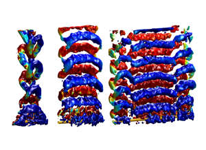
A first overview of the typical wakes associated with the three RBM regimes is proposed in figure 6, through instantaneous iso-surfaces of the $\lambda _2$ criterion (Jeong & Hussain Reference Jeong and Hussain1995), coloured by iso-contours of the spanwise vorticity ($s$ component). Illustrations including wake and cylinder dynamics are also available as supplementary movies 1, 2 and 3 available at https://doi.org/10.1017/jfm.2022.540.

Figure 6. Wake patterns in the RBM regimes. (a) On the left, instantaneous iso-surfaces of the $\lambda _2$ criterion ($\lambda _{2}d^{2}/U^{2} = -0.001$) coloured by iso-contours of the spanwise vorticity ($\omega _{s}d/U \in [-0.1, 0.1]$, blue to red); on the right, particle trajectories coloured by the vertical velocity at $s\approx L/2$, in the R regime ($Ar\simeq 40$, $Re\simeq 42$, $Ca\simeq 15.5$, $L/d\simeq 56$); the cylinder surface is coloured yellow, and its contour is delimited by a black line in the plot on the right. (b) Same as the left-hand plot of (a) in the TRA regime ($d=1.12$ mm, $Ar\simeq 47$, $Re\simeq 49$, $Ca\simeq 2.6$, $L/d\simeq 35$; $d=1.9$ mm, $Ar\simeq 103$, $Re\simeq 124$, $Ca={{O}} (10^{-2})$, $L/d\simeq 10$; $d=2.7$ mm, $Ar\simeq 175$, $Re\simeq 259$, $Ca={{O}} (10^{-5})$, $L/d\simeq 10$), with $\lambda _{2}d^{2}/U^{2} = -0.005$ in the cases depicted in the middle and right-hand panels. (c) Same as the left-hand plot of (a) in the AZI regime ($Ar\simeq 161$, $Re\simeq 217$, $Ca\sim 0$, $L/d\simeq 20$), with $\lambda _{2}d^{2}/U^{2} = -0.005$.

The R regime is encountered at low Reynolds numbers, within the subcritical range where the flow past a rigidly mounted cylinder is expected to be steady in the absence of end effects (Williamson Reference Williamson1996). As discussed in § 5.2, the addition of degrees of freedom to the body may cause flow unsteadiness to appear below the critical $Re$ value of $47$. This is not the case here. No vortex shedding is observed downstream of the cylinder (left-hand plot of figure 6a). The flow is found to be steady and remains essentially symmetrical about the $(s,v)$ plane. This is illustrated further in the right-hand plot of figure 6(a) by a visualization of the flow surrounding the cylinder based on STB trajectories of the seeding tracers.

In the TRA regime, the flow is unsteady and composed of well-defined vortical structures shed downstream of the body. The shape of the vortical structures involved in this regime varies with $L/d$ and $Re$, as shown in figure 6(b). For the cylinder of aspect ratio $L/d=35$, the alternating vortices are parallel to the body axis and present a nearly two-dimensional pattern along most of the span. The spanwise invariance of the vortices ceases near the body ends, where they are bent and connected to the adjacent vortex rows. The region of spanwise invariance tends to vanish when cylinder aspect ratio is reduced, as illustrated in figure 6(b) for $L/d=10$. In this case, the vortices resemble hairpin structures. Similar hairpin structures were reported by Inoue & Sakuragi (Reference Inoue and Sakuragi2008) downstream of stationary low-aspect-ratio cylinders at comparable $Re$ values. The transition between the above-mentioned nearly two-dimensional structures and the hairpin structures appears to be continuous: as the cylinder aspect ratio increases, the spanwise region of the hairpin vortex that is parallel to the body axis widens, leading to an area of parallel shedding. In that sense, the parallel shedding pattern could be regarded as a spanwise-extended version of the hairpin pattern.

The two selected cases of the TRA regime for which $L/d=10$ in figure 6(b) exhibit comparable structural responses and are both characterized by hairpin vortex wakes. They differ essentially by their $Re$ value, $124$ versus $259$. It can be noted that the instantaneous vortex shape becomes less regular as $Re$ increases (the $\lambda _2$ criterion value is the same in both cases); the appearance of such small-scale erratic modulations coincides with the emergence of three-dimensionality of the spanwise vortex rows downstream of a large-aspect-ratio cylinder, close to $Re=180$ (e.g. Williamson Reference Williamson1996). Regardless of the parallel or hairpin shape of the vortices encountered in the TRA regime, the formation and detachment of each vortex from the cylinder seem to occur simultaneously on each side of the body (in the $s$ direction, i.e. $s/L<0.5$ versus $s/L>0.5$); such symmetry in the unsteady flow patterns will be examined in § 4.3.

The typical unsteady wake associated with the AZI regime is depicted in figure 6(c). It is composed mainly of curved spanwise vortices that represent an intermediate state between the parallel and hairpin vortex patterns described previously in the TRA regime. Such an intermediate pattern is expected, considering the intermediate value of the aspect ratio ($L/d=20$). Similar patterns have been reported for comparable aspect ratios by Inoue & Sakuragi (Reference Inoue and Sakuragi2008) (stationary cylinder) and Toupoint et al. (Reference Toupoint, Ern and Roig2019) (freely moving cylinder); it also resembles the oblique shedding pattern described by Williamson (Reference Williamson1989). The value of the Reynolds number in the selected case of the AZI regime, $Re=217$, is close to the value in the last TRA case, visualized in figure 6(b). It can be noted that the irregular small-scale modulations of the vortical structures are analogous in both cases. A major difference with the TRA regime patterns, however, resides in the spanwise antisymmetry of vorticity distribution close to the body. In the AZI regime, the shedding of a given vortex does not occur simultaneously on each side of the cylinder. Instead, the detachment of a positive spanwise vortex ($\omega _s>0$) on one side appears to coincide with the detachment of a negative vortex ($\omega _s<0$) on the other side. This aspect will be analysed in the following.

The above observations concerning the structural responses and global shape of the wake in the different RBM regimes suggest a close connection between body oscillations and flow unsteadiness. An attempt to clarify such a connection is proposed below.

4.3. Flow–structure coupling

The R regime is characterized by the absence of significant body oscillations and by a steady flow; it will not be investigated further.

In order to quantify flow unsteadiness in the TRA and AZI regimes, time series of the horizontal component of flow velocity are collected along a spanwise line located $5$ diameters downstream of the body ($(v,h)=(5,0)$). The frequency spectra of flow velocity fluctuations are plotted along the span in figure 7(a–c), for selected cases (iso-contours). The spanwise modulations in velocity fluctuation intensity reflect the 3-D wake structures depicted in figure 6. In particular, fluctuation intensity tends to drop close to the body ends. A relatively constant level of fluctuation can be noted in the first TRA case (figure 7a), where the flow was found to be invariant (i.e. close to two-dimensional) over most of the span. In spite of the spanwise modulations in fluctuation magnitude, the dominant frequency of flow unsteadiness remains globally constant along the body length, in all cases. Flow unsteadiness frequency varies from one case to the other. Such variation is expected considering the different values of $Re$ and $L/d$, and the distinct dynamics of the body. For comparison purposes, the vortex shedding frequency reported by Williamson & Brown (Reference Williamson and Brown1998) for a fixed cylinder in the absence of end effects is indicated by a black dashed line in each plot.

Figure 7. (a,d,b,e) Flow–structure synchronization in the TRA regime, with: (a,d) $d=1.12$ mm, $Ar\simeq 47$, $Re\simeq 49$, $Ca\simeq 2.6$, $L/d\simeq 35$; and (b,e) $d=1.9$ mm, $Ar\simeq 103$, $Re\simeq 124$, $Ca={{O}} (10^{-2})$, $L/d\simeq 10$. (c,f) Flow–structure synchronization in the AZI regime ($Ar\simeq 161$, $Re\simeq 217$, $Ca={{O}} (10^{-4})$, $L/d\simeq 20$). (a–c) Spanwise evolution of the frequency spectrum (PSD) of the horizontal component of flow velocity sampled 5 diameters downstream of the body. The spectrum amplitudes are normalized by the peak value. In each case, a plain blue line denotes the dominant oscillation frequency identified in figure 5, and a black dashed line indicates the vortex shedding frequency for a long stationary cylinder, $fd/U=0.2731-{1.1129}/{\sqrt {Re}}+{0.4821}/{Re}$ (Williamson & Brown Reference Williamson and Brown1998). In (b), an orange dashed-dotted line indicates the shedding frequency reported by Inoue & Sakuragi (Reference Inoue and Sakuragi2008) for an $L/d = 10$, stationary cylinder at $Re=100$. (d–f) Spanwise evolution of the phases associated with the dominant frequencies of the horizontal component of flow velocity downstream of the body ($u'_{h}$) and of the horizontal oscillation; the phases are centred about their span-averaged values.

The span-averaged dominant frequency of cylinder horizontal oscillation is superimposed on flow velocity spectra in figure 7(a–c) (plain blue lines). Body oscillation frequency and flow unsteadiness frequency are found to coincide at each spanwise location. Body motion and flow unsteadiness are thus synchronized, a condition generally referred to as lock-in in the context of vortex-induced vibrations of elastically mounted bodies (Williamson & Govardhan Reference Williamson and Govardhan2004). Flow–body synchronization is established in all studied cases of TRA and AZI regimes.

Synchronization mechanisms can be analysed further by comparing the spanwise evolutions of the phases associated with the dominant frequencies of body responses and flow velocity fluctuations. These phases are plotted in figure 7(d–f), for each selected case; as in figure 5, the phases are centred about their span-averaged values. In the TRA regime, flow fluctuation phase remains close to constant over a wide region about the midspan point, as body response phase. This corroborates the above observation based on instantaneous visualizations, concerning the symmetry of vortical structure formation along the span, i.e. simultaneous shedding in the $s/L<0.5$ and $s/L>0.5$ regions. The phase opposition between each side of the cylinder, associated with the AZI regime responses, can also be noted in flow unsteadiness (even though defined less clearly). Such distribution of the phase confirms the above-mentioned antisymmetry of the wake dynamics (opposite sign vortices shed simultaneously on each side), which is thus found to match the antisymmetry of body rotary oscillation. Phase analysis shows that body motion and flow unsteadiness are not only temporally synchronized but also spatially locked to each other.

This spatio-temporal synchronization could explain the spanwise distribution of flow fluctuation intensity visualized in figure 7(c) for the AZI regime: intensity peaks appear close to $s/L=0.21$ and $L/d=0.73$, i.e. in regions of significant structural response amplitudes (but far enough from the body ends, where fluctuation intensity is low in all studied cases); the central region, where the rotary motion results in lower oscillation amplitudes, exhibits lower intensity fluctuations of flow velocity.

A complementary vision of flow–body synchronization in the TRA and AZI regimes is presented in figure 8, where phase-averaged (using between 3 and 4 cycles) iso-contours of the spanwise vorticity are plotted in selected planes perpendicular to the cylinder axis, for two typical cases. The selected planes correspond to the body ends and midspan point, as well as the regions where flow fluctuation intensity peaks in the AZI regime case (figure 7c). The phase-averaging process is based on body response. The phase depicted in figure 8 is chosen arbitrarily and corresponds to the phase of the cycle where body oscillation amplitude vanishes. The fact that vortex shedding is captured by the phase-averaging process suggests that it is synchronized with body motion.

Figure 8. Phase-averaged vortex shedding process in (a) the TRA regime ($d=1.9$ mm, $Ar\simeq 103$, $Re\simeq 124$, $Ca={{O}} (10^{-2})$, $L/d\simeq 10$), and (b) the AZI regime ($d=2.55$ mm, $Ar\simeq 161$, $Re\simeq 217$, $Ca={{O}} (10^{-4})$, $L/d\simeq 20$). Phase-averaged iso-contours of the spanwise vorticity ($\omega _{s} d/U \in [-1,1]$, blue to red) are plotted in selected planes perpendicular to the cylinder axis, $s/L \simeq 0, 0.21, 0.5, 0.73, 1$. The selected phase corresponds to the phase of the cycle where the amplitude of oscillation vanishes. In each plot, a horizontal segment (barely visible) denotes the cylinder trajectory.

At $s/L=0.21$ and $L/d=0.73$, the planar structure of the wake resembles the 2S pattern, with two counter-rotating vortices shed per oscillation cycle (Williamson & Govardhan Reference Williamson and Govardhan2004), regardless of the 3-D shape of the overall vortical structure (e.g. hairpin). A comparison of the vorticity fields at these spanwise locations shows that the alternately shed vortices are in phase in the TRA regime and in phase opposition in the AZI regime, thus matching body response phasing. As also observed in the instantaneous visualizations in figure 6, the alternating vortex shedding ceases in the cylinder end regions. At the midspan point, in the AZI regime, the alternating shedding is expected to be replaced by the simultaneous shedding of opposite sign vortices, as reported previously near vibration nodes for flexible cylinders (e.g. figure 12 in Newman & Karniadakis Reference Newman and Karniadakis1997). Such a pattern is not observed in the present case where the phase opposition between vortex formation on each side of the body is accommodated by a global asymmetrical wake structure, as discussed in the following; such an asymmetrical structure differs from the strictly antisymmetrical structure reported by Newman & Karniadakis (Reference Newman and Karniadakis1997).

To visualize further the wake dynamics associated with the AZI regime, instantaneous iso-surfaces of the $\lambda _2$ criterion coloured by iso-contours of spanwise vorticity are plotted in figure 9, at five selected instants over one oscillation cycle. The different instants are indicated in figure 9(a), which represents selected time series of cylinder horizontal displacement at $s=0$ and $s=L$, i.e. body ends. Based on these visualizations and on the phasing identified in figure 7( f), the following scenario can be proposed to describe wake dynamics. Each vortex starts to detach from the cylinder in the central region. As it is convected downstream, the vortex is progressively peeling off from the body, towards its ends. This process is comparable to the hairpin vortex formation observed in the TRA regime (figure 6b). However, in the AZI regime, the propagation of the detachment points of the vortex, from the central region towards each end, is not strictly symmetrical for $s/L<0.5$ and $s/L>0.5$, so that the vortex detaches from one end while it is still attached to the body at the other end. Such a time difference in vortex detachment can be visualized at instant A (figure 9b): the blue vortex that is close to be shed but still attached near the left end (green arrow) has already been shed on the right side of the body (orange arrow). As a result, the bent vortices observed in the wake are not symmetrical about the midspan point, and they appear to be slightly inclined in the $(s,v)$ plane. A comparable asymmetry/inclination can be noted in the dye visualization reported by Toupoint et al. (Reference Toupoint, Ern and Roig2019) (figure 17c in that paper). The above described process repeats successively for the positive and negative vortices, so that positive and negative vortices are formed and then shed simultaneously from each side of the cylinder, leading to the phase opposition mentioned previously. At instant A in the flow visualization of figure 9(b–f), a red vortex is close to be shed near the right end of the body (black arrow), simultaneously with the blue vortex indicated by a green arrow near the left end.

Figure 9. Wake dynamics in the AZI regime ($d=2.55$ mm, $Ar\simeq 161$, $Re\simeq 217$, $Ca={{O}} (10^{-4})$, $L/d\simeq 20$). (a) Time series of cylinder horizontal displacement at $s=0$ (blue) and $s=L$ (orange). (b–f) Instantaneous iso-surfaces of the $\lambda _2$ criterion ($\lambda _{2}d^{2}/U^{2} = -0.03$) coloured by iso-contours of spanwise vorticity ($\omega _{s}d/U\in [-0.1, 0.1]$, blue to red), at the five selected instants indicated in (a).

To summarize, the R regime where no significant structural responses emerge is associated with a steady flow. The typical translatory and rotary responses of the TRA and AZI regimes are restricted essentially to the horizontal plane; they are close to periodic and exhibit limited amplitudes, of the order of $0.03$ body diameters. Both regimes involve a condition of spatio-temporal synchronization between body oscillations and flow unsteadiness. The TRA regime may develop under a variety of flow patterns, globally symmetrical about the midspan point, and ranging from spanwise-invariant vortex rows to hairpin vortex shedding. These patterns are all associated with a phase of flow velocity fluctuations that remains constant along a portion of the span about the midspan point, as body response phase. In contrast, the AZI regime is accompanied by an asymmetrical shedding pattern that results in an antisymmetrical distribution of spanwise vorticity and a phase opposition between flow velocity fluctuations on each side of the body, which matches the body behaviour phasing.

5.1. Structural responses

The bending oscillations of the cylinder in the selected cases of the M$_1$ and M$_2$ regimes are quantified in figure 10. Supplementary movie 4 depicts the cylinder oscillations during its fall under the M$_1$ regime.

Figure 10. Structural responses in the BO regimes. (a,c) Spanwise evolution of the time-averaged amplitude of oscillation and (b,d) span-averaged frequency spectrum (PSD) of the oscillation, in the horizontal (plain line) and vertical (dashed line) directions, in (a,b) the M$_1$ regime ($Ar\simeq 45$, $Re\simeq 42$, $Ca\sim 36$, $L/d\simeq 68$) and (c,d) the M$_2$ regime ($Ar\simeq 40$, $Re\simeq 37$, $Ca\sim 210$, $L/d\simeq 107$). In (b,d), the oscillation frequencies reported in Ern et al. (Reference Ern, Mougel, Cazin, Lorite-Díez and Bourguet2020) based on shadowgraphy experiments, for the same cylinders, are indicated by red dashed-dotted lines, and the natural frequencies of the first and second structural modes, computed as $f_i = \alpha _i d/L^2 \sqrt {E/(\rho _c+\rho _f)}$, with $\alpha _1 \approx 0.890$ and $\alpha _2 \approx 2.454$, respectively, are denoted by purple lines.

The fact that the successive minima of the horizontal response envelopes (figure 10a,c) are close to zero amplitude indicates that the structural oscillations occurring in this direction consist mainly of standing waves. The succession of nodes and crests reflects the shape of the structural mode involved in each case: the first mode with two nodes, and the second mode with three nodes. Vertical response amplitudes exhibit tangible spanwise modulations that betray the presence of bending oscillations also in this direction. However, no clear topology of response shapes can be established, and no dominant structural mode emerges. As in the RBM regimes, the horizontal responses are much larger than the vertical ones, and the body appears to oscillate essentially in the horizontal plane. It should, however, be mentioned that the responses encountered in the BO regimes, typically close to $0.3$ and $0.02$ diameters in the horizontal and vertical directions, respectively, are one order of magnitude larger than those observed in the RBM regimes. These BO amplitudes are comparable to those usually reported for elastically mounted rigid cylinders and pinned flexible cylinders subjected to vortex-induced vibrations at similar $Re$ values (e.g. Mittal & Singh Reference Mittal and Singh2005; Bourguet Reference Bourguet2020).

The span-averaged spectra of the horizontal and vertical oscillations are plotted in figure 10(b,d). In both directions, the responses are close to periodic. The horizontal oscillations are dominated by a single frequency, as in the RBM regimes. This frequency, close to $f d/U=0.13$ in each case, coincides with that issued from shadowgraphy measurements (Ern et al. Reference Ern, Mougel, Cazin, Lorite-Díez and Bourguet2020), shown with red dashed-dotted lines in figure 10(b,d). It may deviate from the natural frequency of the corresponding structural mode ($f_1 d/U=0.107$ in the first case, and $f_2 d/U=0.126$ in the second case, where the added mass coefficient is estimated by its potential flow value of $1$; purple solid lines in the plots).

Such a departure from the natural frequency is a typical phenomenon, often associated with the lock-in mechanism, especially at low mass ratios (Williamson & Govardhan Reference Williamson and Govardhan2004; Bourguet et al. Reference Bourguet, Karniadakis and Triantafyllou2011a). This aspect will be addressed in § 5.3. Due to the (theoretical) symmetry of the physical system and the ratio of $2$ between the streamwise and transverse fluid forcing for a rigidly mounted circular cylinder, the vertical oscillations are expected to occur at twice the horizontal response frequency. These components indeed appear in response spectra (figure 10b,d), but they are accompanied by first harmonic contributions, which actually dominate the response spectrum in the M$_2$ regime case. The combination of first and second harmonic contributions to streamwise structural dynamics is observed frequently for supported flexible cylinders subjected to vortex-induced vibrations (Huera-Huarte & Bearman Reference Huera-Huarte and Bearman2009; Seyed-Aghazadeh, Edraki & Modarres-Sadeghi Reference Seyed-Aghazadeh, Edraki and Modarres-Sadeghi2019); this may be attributed to slight asymmetries in the experimental configuration (e.g. small permanent deformation, not strictly circular cross-section, etc.) but also to spontaneous symmetry breaking in the system response, due for instance to the incompatibility between the fluid forcing frequency and the shape of the corresponding mode (Gedikli, Chelidze & Dahl Reference Gedikli, Chelidze and Dahl2018), as well as the possible emergence of asymmetrical vortex shedding patterns (Singh & Mittal Reference Singh and Mittal2005).

The phases associated with the dominant frequencies of the horizontal and vertical responses are represented along the span in figure 11(a,c), for the selected cases. In each case, the phase of the horizontal response ($\varphi _h$) is a constant piecewise function of $s$, with ${\rm \pi}$ jumps at the nodes. Such a phase distribution confirms the standing wave nature of the oscillation. In the vertical direction, the phases associated with the first ($\varphi _{v1}$) and second ($\varphi _{v2}$) harmonics exhibit less clearly defined evolutions. The first harmonic components appear to be mixtures of standing and travelling wave patterns, while the phases of the second harmonic components remain relatively constant along the span; in both cases, the second harmonic contribution could thus be regarded as an RBM, modulated slightly along the span.

Figure 11. Phasing of the structural responses in (a,b) the M$_1$ regime ($Ar\simeq 45$, $Re\simeq 42$, $Ca\sim 36$, $L/d\simeq 68$), and (c,d) the M$_2$ regime ($Ar\simeq 40$, $Re\simeq 37$, $Ca\sim 210$, $L/d\simeq 107$). (a,c) Spanwise evolution of the phases associated with the dominant frequency of the horizontal oscillation ($\varphi _{h}$) and the first and second harmonics of the vertical oscillation ($\varphi _{v1}$, $\varphi _{v2}$), as well as the phase difference $\varphi _{vh}=\varphi _{v2}-2\varphi _{h}$. (b,d) Probability density function (p.d.f.) of the phase difference $\varphi _{vh}$ between the horizontal and vertical responses; shaded areas indicate the dominant phase difference range reported in Bourguet (Reference Bourguet2020) for pinned flexible cylinders. In (b), the inset represents the horizontal versus second harmonic vertical responses (i.e. filtered orbit) at $s=L/2$ in the M$_{1}$ regime ($\varphi _{vh} = 0.18$).

The phasing of the horizontal and vertical responses determines, at each spanwise location, the shape of cylinder trajectory. Previous studies concerning vortex-induced vibrations of rigid and flexible cylinders have shown that trajectory shape is linked closely to flow–structure energy transfer (i.e. excitation/damping of the structure by the flow) and that some shapes are more likely to occur under lock-in (Dahl et al. Reference Dahl, Hover, Triantafyllou and Oakley2010; Bourguet et al. Reference Bourguet, Modarres-Sadeghi, Karniadakis and Triantafyllou2011b; Fan et al. Reference Fan, Wang, Triantafyllou and Karniadakis2019). For a frequency ratio of $1$ between the vertical and horizontal responses, the cylinder exhibits elliptical trajectories, while it describes figure-eight orbits when the frequency ratio is equal to $2$. In the present cases, where both first and second harmonic contributions arise in the vertical response spectra, the trajectory is a figure-eight with unequal loop sizes. In a recent work concerning pinned flexible cylinders at comparable $Re$, a dominant trajectory shape was identified over wide ranges of body aspect ratios and excited modes (Bourguet Reference Bourguet2020). This dominant trajectory consists of a figure-eight shape, close to a crescent bent downstream (i.e. upwards), where the body moves upstream when reaching transverse oscillation maxima; such an orbit orientation was referred to as counter-clockwise in prior studies (Dahl et al. Reference Dahl, Hover, Triantafyllou and Oakley2010).

For comparison purposes with this persistent phasing mechanism, focus is placed here on the phase difference between the horizontal response and the second harmonic of the vertical response, $\varphi _{vh}=\varphi _{v2}-2\varphi _{h}$. For each selected case, this phase difference is computed at each spanwise location (figure 11a,c), and the corresponding probability density functions (p.d.f.) are plotted in figure 11(b,d). In each case, the phase difference is found to be restricted to a narrow range, and it can be observed that this range coincides closely with that identified in Bourguet (Reference Bourguet2020) (shaded areas in the plots). The typical, dominant trajectory of the body is visualized in the inset of figure 11(b) at the midspan point, in the M$_1$ regime case. It is recalled that the vertical oscillations examined here exhibit low amplitudes and involve both first and second harmonic contributions. However, the present results confirm previous observations and suggest that the phasing mechanism of the horizontal and vertical responses could be a generic feature for flexible cylinders subjected to bending oscillations in this $Re$ range, regardless of the supported or unsupported end conditions and the structural modes at play.

5.2. Flow patterns

The cases of M$_1$ and M$_2$ regimes examined here are characterized by low Reynolds number values, $Re=42$ and $Re=37$, respectively. For a rigidly mounted cylinder and in the absence of end effects, the flow is expected to be steady in this $Re$ range (Williamson Reference Williamson1996). However, prior works have shown that when one or more degrees of freedom are added to the structure, the flow may become unsteady at much lower $Re$ than the critical value of $47$, typically down to $Re \approx 20$ depending on $m^*$. Such a phenomenon was reported for rigid cylinders (Cossu & Morino Reference Cossu and Morino2000; Mittal & Singh Reference Mittal and Singh2005; Meliga & Chomaz Reference Meliga and Chomaz2011; Dolci & Carmo Reference Dolci and Carmo2019; Boersma et al. Reference Boersma, Zhao, Rothstein and Modarres-Sadeghi2021), as well as pinned flexible cylinders (Bourguet Reference Bourguet2020); it was also conjectured to occur for freely falling flexible cylinders in Ern et al. (Reference Ern, Mougel, Cazin, Lorite-Díez and Bourguet2020), based on bending oscillations measurements only. The present measurements confirm that the flows associated with the selected cases of BO regimes are unsteady, despite the low $Re$ values.

The typical wake patterns encountered downstream of the oscillating cylinder in the M$_1$ and M$_2$ regimes are visualized in figure 12 via instantaneous iso-surfaces of the $\lambda _2$ criterion, coloured by iso-contours of the spanwise vorticity, as in figure 6. Illustrations including wake and cylinder dynamics for the two BO regimes are available in supplementary movies 5 and 6. A first overview of these visualizations indicates that wake patterns are composed mainly of regularly shed, spanwise vortex rows globally parallel to the cylinder axis. These vortex rows and their connections close to the body ends resemble those depicted in figure 6(b) in the TRA regime, for $L/d=35$. A closer examination, however, reveals some subtle differences. Two elements can be noted. First, slight distortions of the successive vortex rows appear at specific spanwise locations, which seem to coincide with the nodes of the horizontal structural responses. Second, on each side of these distortion points, positive vortex rows are found to be roughly aligned with negative vortex rows, i.e. a phase shift close to ${\rm \pi}$ occurs in the wake at these locations as observed previously for the AZI mode. These elements as well as the value of the body oscillation frequency, close to the vortex shedding frequency reported at comparable $Re$ by Buffoni (Reference Buffoni2003), indicate a link between body motion and flow unsteadiness, as in the RBM regimes and as also hypothesized in Ern et al. (Reference Ern, Mougel, Cazin, Lorite-Díez and Bourguet2020).

Figure 12. Wake patterns in the BO regimes. Instantaneous iso-surfaces of the $\lambda _2$ criterion ($\lambda _{2}d^{2}/U^{2} = -0.001$) coloured by iso-contours of the spanwise vorticity ($\omega _{s}d/U\in [-0.1, 0.1]$, blue to red) for (a) the M$_1$ regime ($Ar\simeq 45$, $Re\simeq 42$, $Ca\sim 36$, $L/d\simeq 68$), and (b) the M$_2$ regime ($Ar\simeq 40$, $Re\simeq 37$, $Ca\sim 210$, $L/d\simeq 107$).

5.3. Flow–structure coupling

The procedure introduced in § 4.3 to clarify the connection between solid behaviour and flow unsteadiness in the RBM regimes is applied here to the selected M$_1$ and M$_2$ regime cases. For each case, the frequency spectra of the horizontal flow velocity fluctuations, collected $5$ diameters downstream of the cylinder, are plotted along the span in figure 13(a,b), together with the horizontal deformation frequency (plain blue line).

Figure 13. Same as figure 7 in (a,c) the M$_1$ regime ($Ar\simeq 45$, $Re\simeq 42$, $Ca\sim 36$, $L/d\simeq 68$), and (b,d) the M$_2$ regime ($Ar\simeq 40$, $Re\simeq 37$, $Ca\sim 210$, $L/d\simeq 107$). The natural frequencies of the first and second structural modes are denoted by plain purple lines in (a,c) and (b,d), respectively. The vortex shedding frequencies reported by Buffoni (Reference Buffoni2003) at subcritical $Re$, for rigid circular cylinders, are indicated by black dashed lines.

The spectral amplitudes of flow velocity fluctuations exhibit large spanwise modulations, but their dominant frequency remains constant and matches the structural oscillation frequency throughout the body length. In each case, this temporal synchronization occurs at a frequency that departs slightly from the structure natural frequency ($f_1$ or $f_2$, plain purple line). A slight deviation from the vortex shedding frequency identified by Buffoni (Reference Buffoni2003) (black dashed line) can also be noted.

The phases associated with the horizontal oscillation and flow fluctuation frequencies are plotted in figure 13(c,d). The phases are centred about their span-averaged values; the fact that the relative phase at $s=0$ is the same in $M_2$ and different in $M_1$ is related to the chosen wake position. Phase comparison shows that a phase jump occurs in the flow at each node of the structural response. More precisely, it indicates that flow velocity fluctuations are in phase opposition on each side of the nodes, which confirms the above-mentioned phase opposition in vortex distribution along the span, i.e. the successive alignment of negative and positive vortices on each side of the nodes. As also observed in the RBM regimes, the intensity of flow unsteadiness tends to drop near the body ends. Away from the ends, flow unsteadiness intensity is found to follow the local amplitude of the structural response. In particular, minima and maxima of flow velocity fluctuations are observed near the nodes and antinodes of the horizontal response, respectively.

Therefore, body motion and flow unsteadiness are both temporally and spatially locked, as in the RBM regimes. This spatio-temporal lock-in mechanism involving bending oscillations of the body was described previously at comparable $Re$, for pinned cylinders (Bourguet Reference Bourguet2020). The present results show that such a synchronization mechanism may also occur for unsupported, freely falling cylinders.

The spatio-temporal lock-in mechanism is accompanied by a cellular structure of the wake where each cell is delimited by the horizontal deformation nodes. A visualization of these patterns is presented in figure 14 via phase-averaged iso-surfaces of spanwise vorticity. As in figure 8, the phase-averaging process is based on the horizontal response of the body (using between 7 and 8 cycles), and the selected phase corresponds to the phase of the cycle where the response vanishes. In the $(s,v)$ and $(h,s)$ plane visualizations (figure 14), the spanwise locations of the horizontal response nodes are indicated by green dashed lines. Complementary side views show the interconnections of the successive vortex rows in the cylinder end region (figure 14, lateral views). Figure 14 can be examined together with figure 15, which represents iso-contours of the phase-averaged spanwise vorticity field in selected planes along the span. The planes are located at the body end and at horizontal vibration nodes and antinodes, over half of the span. The selected phases correspond to maximum and minimum amplitudes of horizontal oscillation, as indicated by cylinder position in each plot.

Figure 14. Phase-averaged flow patterns in (a) the M$_1$regime ($Ar\simeq 45$, $Re\simeq 42$, $Ca\sim 36$, $L/d\simeq 68$), and (b) the M$_2$regime ($Ar\simeq 40$, $Re\simeq 37$, $Ca\sim 210$, $L/d\simeq 107$). Frontal, vertical (at $v/d\simeq 5$) and lateral views of the phase-averaged iso-surfaces of the $\lambda _2$ criterion ($\lambda _{2}d^{2}/U^{2}$ = $-8\times 10^{-4}$) are shown, coloured by iso-contours of the spanwise vorticity ($\omega _s\in [-0.08, 0.08]$, blue to red). The selected phase corresponds to the phase of the oscillation cycle where the horizontal response vanishes. In frontal and vertical views, the spanwise locations of the horizontal response nodes are indicated by green dashed lines.

Figure 15. Same as figure 8 in (a) the M$_1$ regime ($Ar\simeq 45$, $Re\simeq 42$, $Ca\sim 36$, $L/d\simeq 68$), and (b) the M$_2$ regime ($Ar\simeq 40$, $Re\simeq 37$, $Ca\sim 210$, $L/d\simeq 107$), with $\omega _{s}d/U \in [-0.3, 0.3]$. For each case, the selected planes are indicated in a sketch (top) which represents the amplitude of the horizontal oscillation, over half of the cylinder span.

The 3-D visualizations in figure 14 (frontal views) show evidence of the local distortions of the spanwise vortices near response nodes, as well as their relatively spanwise-invariant shape in-between. Within each cell, i.e. between two successive nodes, figure 15 shows that two counter-rotating vortices form per oscillation cycle (2S pattern; Williamson & Govardhan Reference Williamson and Govardhan2004). The phase of flow velocity fluctuations may exhibit some variations in each cell (figure 13c,d) which is reflected in the wake by a slight streamwise bending of the vortical structures (e.g. for $s/L\in [0.2,0.5]$ in the M$_2$ regime case). On each side of a node, a positive vortex is found to coincide with a negative vortex, as mentioned previously. This global phase opposition is confirmed by the antisymmetrical structures of the vorticity fields represented in figure 15. The alignment of the adjacent vortex rows is, however, not perfect, as expected from the phase plots in figure 13(c,d): the phase jumps of the wake at the nodes are generally not strictly equal to ${\rm \pi}$, contrary to those observed for the body responses. Another asymmetry can be noted, in the interconnection between the same-sign vortex rows. For comparable cellular patterns, prior works showed that each vortex row is connected, across the node region, to the previous and next vortex rows (e.g. figure 4 in Bourguet Reference Bourguet2020). Here, generally, a single connection is observed, either with the previous or with the next adjacent vortex. This symmetry breaking in vortex connection is associated with the absence of symmetrical shedding patterns near the nodes, as those visualized by Newman & Karniadakis (Reference Newman and Karniadakis1997); as a result, even in the node regions, wake shape resembles the 2S pattern (see figure 15, for instance). The above-mentioned misalignment of vortex rows and asymmetries might be attributed to imperfections of the experimental configuration (e.g. small static deformation of the cylinder, slight inclination of the body as it falls, etc.). These asymmetries, however, have a limited impact on the overall structure of the cellular wake patterns encountered in the M$_1$ and M$_2$ regimes, which remain close to those associated with the occurrence of standing wave responses under lock-in, for pinned flexible cylinders (Bourguet Reference Bourguet2020).

Previous studies concerning cylinders subjected to forced oscillations have emphasized the influence of oscillation properties (amplitude, frequency) on the shape of the recirculation region appearing in the near wake (e.g. Ramberg & Griffin Reference Ramberg and Griffin1974). The length of the recirculation region is particularly significant as it is related directly to the local drag force (Roshko Reference Roshko1993). Based on flow visualizations comparable to that presented in figure 6(a), the recirculation length, $L_r$, is measured at each spanwise location, as the streamwise distance between the cylinder surface and the point where $|u_{v}|>U$, i.e. the relative time-averaged (§ 3.2) vertical flow velocity with respect to the body changes sign. The spanwise distribution of $L_r$ is plotted in figure 16(c) for the M$_1$ and M$_2$ regimes. In spite of the dispersion inherent in the measurement technique (lack of seeding particles inside the recirculation region), a trend can be identified: the recirculation length tends to increase near the structural response nodes (vertical dashed lines) and to decrease in larger-amplitude response regions. To clarify this phenomenon, the recirculation lengths measured in both cases are plotted as functions of the local oscillation amplitude in figure 16(c). A global decrease of $L_r$ is noted as oscillation amplitude increases; a similar trend was reported by Ramberg & Griffin (Reference Ramberg and Griffin1974) under forced vibrations. The size of the recirculation region is thus modulated along the span, and its modulation coincides locally with the deformation amplitude. This observation sheds light on another aspect of the close connection between body oscillation and wake structure. Due to the low amplitudes of the responses and the dispersion of $L_r$ values, it was not possible to establish clearly a comparable behaviour for the RBM regimes, even though it is likely to persist in these regimes, as suggested by the low-amplitude results in the above-mentioned study.

Figure 16. Evolution of the recirculation length, (a,b) along the span, and (c) as a function of the horizontal oscillation amplitude, in the M$_1$ regime ($Ar\simeq 45$, $Re\simeq 42$, $Ca\sim 36$, $L/d\simeq 68$, blue) and the M$_2$ regime ($Ar\simeq 40$, $Re\simeq 37$, $Ca\sim 210$, $L/d\simeq 107$, red). In (a,b), the locations of the horizontal response nodes are indicated by black dashed lines, and plain lines denote the span-averaged value of the recirculation length.

The principal features of the BO regimes examined in this section can be summarized as follows. As in the RBM regimes, body oscillations are close to periodic and occur essentially in the horizontal plane; yet their amplitudes are one order of magnitude larger, typically close to $0.3$ and $0.02$ diameters in the horizontal and vertical directions, respectively. The horizontal and vertical responses exhibit a specific phasing that matches that identified previously for pinned flexible cylinders. As also observed in the RBM regimes, the structural responses develop under a condition of spatio-temporal synchronization between the moving body and the flow, which is found to be unsteady, even though the Reynolds number is subcritical. The synchronization of the spanwise structure of the flow with the horizontal, standing wave responses of the body is accompanied by the formation of cellular patterns in the wake. Each cell consists of alternately shed spanwise vortex rows, globally aligned with the cylinder. The adjacent vortex rows are interconnected in response node regions where the phase shift of flow velocity fluctuations and antisymmetrical vorticity distribution coincide with response phase opposition. The close relation between body motion and wake organization is illustrated further by the joint evolution of the local amplitude of the body response and recirculation length.