


1 Introduction
Third-order nonlinear wave–wave interactions are key for the evolution of ocean wave sea states, whereas second-order interactions only produce local trough–crest asymmetry. For wave–structure interactions, second-order processes produce excitation at both paired sum and difference frequencies, and these are practically important for a whole range of structural responses. Examples include slow drift of moored vessels, springing of ship hulls, enhanced water elevation between the legs of semi-subs and tension leg platforms. There has been very little work on third-order diffraction through the solution of Stokes-like perturbation problems other than some work on the ringing of columns, e.g. Faltinsen, Newman & Vinje (Reference Faltinsen, Newman and Vinje1995), Malenica & Molin (Reference Malenica and Molin1995), and this has focused on the triple frequency sum terms.
It has been well known for many years that, when two trains of waves in deep water interact, the phase velocity of each is modified by the presence of the other through tertiary wave interactions (Longuet-Higgins & Phillips Reference Longuet-Higgins and Phillips1962). The change of phase velocity is of second order in wave steepness, occurring for each Fourier component due to the presence of all other components. Thus it is distinct from the increase in a Stokes regular wave train which occurs due to self-interaction only. The possible implications of such tertiary interaction effects had never been considered for wave–structure problems until Molin et al. (Reference Molin, Remy, Kimmoun and Ferrant2003), although much work has been done on third-order wave–wave interactions since the early papers by Phillips and Longuet-Higgins (Phillips Reference Phillips1981).
Based on a series of regular wave tests, Molin et al. (Reference Molin, Remy, Kimmoun and Ferrant2003) reported a large wave run-up phenomenon where the local wave surface elevations at the front face of a vertical plate reached
 $4\times$
or
$4\times$
or
 $5\times$
the amplitude of the incident waves, much larger than the
$5\times$
the amplitude of the incident waves, much larger than the
 ${\sim}2\times$
predicted from linear theory. It was proposed (Molin et al.
Reference Molin, Remy, Kimmoun and Ferrant2003, Reference Molin, Remy, Kimmoun and Jamois2005) that the large wave run-ups result from the tertiary wave interactions of Longuet-Higgins & Phillips (Reference Longuet-Higgins and Phillips1962), in such a way that the reflected wave fields from the body slow down the incident waves as a shoal would locally. This leads to locally curved wave fronts and local energy concentration in front of the body – this process we describe as Molin lensing. It further induces wave focusing on the weather side of the structure, leading to significant wave run-up enhancement. Following these interesting observations, more experiments were performed using fixed vertical plates of different sizes to confirm the amplification phenomenon, as summarized in Molin et al. (Reference Molin, Kimmoun, Remy and Chatjigeorgiou2014). Numerical models have been developed to predict the measured profiles along fixed vertical plates (Molin et al.
Reference Molin, Kimmoun, Liu, Remy and Bingham2010): the parabolic model of Molin et al. (Reference Molin, Remy, Kimmoun and Jamois2005) based on the tertiary theories of Longuet-Higgins & Phillips (Reference Longuet-Higgins and Phillips1962) and fully nonlinear numerical wave tanks based on extended Boussinesq equations (Bingham et al.
Reference Bingham, Fuhrman, Jamois and Kimmoun2004) and potential flow theory (Jamois et al.
Reference Jamois, Fuhrman, Bingham and Molin2006). These studies have confirmed the important role of the tertiary interactions in producing large wave run-up phenomena, but in regular waves only.
${\sim}2\times$
predicted from linear theory. It was proposed (Molin et al.
Reference Molin, Remy, Kimmoun and Ferrant2003, Reference Molin, Remy, Kimmoun and Jamois2005) that the large wave run-ups result from the tertiary wave interactions of Longuet-Higgins & Phillips (Reference Longuet-Higgins and Phillips1962), in such a way that the reflected wave fields from the body slow down the incident waves as a shoal would locally. This leads to locally curved wave fronts and local energy concentration in front of the body – this process we describe as Molin lensing. It further induces wave focusing on the weather side of the structure, leading to significant wave run-up enhancement. Following these interesting observations, more experiments were performed using fixed vertical plates of different sizes to confirm the amplification phenomenon, as summarized in Molin et al. (Reference Molin, Kimmoun, Remy and Chatjigeorgiou2014). Numerical models have been developed to predict the measured profiles along fixed vertical plates (Molin et al.
Reference Molin, Kimmoun, Liu, Remy and Bingham2010): the parabolic model of Molin et al. (Reference Molin, Remy, Kimmoun and Jamois2005) based on the tertiary theories of Longuet-Higgins & Phillips (Reference Longuet-Higgins and Phillips1962) and fully nonlinear numerical wave tanks based on extended Boussinesq equations (Bingham et al.
Reference Bingham, Fuhrman, Jamois and Kimmoun2004) and potential flow theory (Jamois et al.
Reference Jamois, Fuhrman, Bingham and Molin2006). These studies have confirmed the important role of the tertiary interactions in producing large wave run-up phenomena, but in regular waves only.
It has been 15 years since the pioneering work of Molin et al. (Reference Molin, Remy, Kimmoun and Ferrant2003). Surprisingly limited attention has been paid to the tertiary interaction phenomena other than in generalizations of the Benjamin–Feir instability in undisturbed wave fields. We also note that all the literature available for enhanced wave run-ups has focused on regular waves only, both seeking a steady-state solution and investigating the time evolution of the free-surface elevation. Therefore, there are some important open questions remaining, particularly for waves in a random sea, e.g. (i) whether the tertiary interactions are important; (ii) if so, how to identify the time evolution of wave run-up amplification and phase or time lag in a random signal.
In light of these questions, we carried out a set of experiments using different types of waves but all with normal incidence, to investigate the wave run-up in front of a fixed box. The theory of the average shape of large events in a random process, the so-called NewWave theory (Jonathan & Taylor Reference Jonathan and Taylor1997), is applied to highlight possible tertiary interaction effects in a random sea. This study is organized as follows. Following this introduction, the experimental set-up in a wave basin is described in § 2. Regular wave test results are presented in § 3, showing very similar observations to those in Molin et al. (Reference Molin, Remy, Kimmoun and Jamois2005) for a vertical plate, confirming that the same effects are being produced in our tests. Results from transient wave group tests are given in § 4. No tertiary interaction phenomena are observed as there is little opportunity for interactions between the incident and reflected waves upstream of the structure. However, the analysis of the deterministic transient wave groups significantly facilitate the presentation of the irregular wave results which are given in § 5. First, the time evolution of the wave surface elevations at the centre of the front face of the fixed box is identified in § 5.1 through spectral analysis of individual time windows. Then, we run NewWave-type analysis in § 5.2 where a net phase or time lag, a key characteristic of the tertiary interactions, is identified for the random signals. The spatial structure of the wave field associated with enhanced run-up is analysed in § 5.3. Some evidence is provided in appendix A to eliminate possible concern that there might be tank resonances or standing waves between the wave paddles and the fixed box. Finally the conclusions are described in § 6.

Figure 1. Experimental set-up: (a) sketch (not to scale) of the fixed box in the wave basin, with the red crosses showing the locations of the wave probes; (b) a snapshot of the wave field in front of the fixed box hull (yellow) rigidly connected to the gantry (blue).
2 Experimental set-up
The experiments were carried out in the Deepwater Wave Basin at Shanghai Jiao Tong University. The wave basin is 50 m long, 40 m wide and the water depth was set to 10 m. Flap-hinged wavemakers are installed along two neighbouring sides of the basin and wave absorbing beaches are fixed on the opposite sides to minimize reflected waves from the boundaries of the basin.
The experimental set-up is identical to that described in Zhao et al. (Reference Zhao, Wolgamot, Taylor and Eatock Taylor2017), where the object of the tests was to investigate the resonant fluid responses in narrow gaps between two side-by-side moored boxes. Two identical 3.333 m long and 0.767 m wide rectangular boxes were used, these were 0.425 m high and immersed such that the undisturbed draught was 0.185 m. In cross-section the models have round corners at both bilges, each with a radius of 0.083 m running along the length. As shown in figure 1, the two boxes were rigidly mounted to a gantry in the centre area of the wave basin in a side-by-side configuration, forming a narrow gap of 0.067 m. The midpoint of the gap was 19.83 m away from the wave paddles and 20 m from the side walls of the wave basin. The gantry is very robust, so provided enough stiffness to prevent vibrations of the models at wave frequencies. Gap resonances do not significantly affect the wave field on the weather side of the boxes, this is demonstrated in § 5.1. Therefore, the two identical boxes in side-by-side configuration with a narrow gap is equivalent to a single ‘flat’ box of width
 $2\times 0.767+0.067=1.601$
m, from the perspective of wave run-up and reflection on the weather side. For clarity, we do not show the location of the wave gauges in the gap, but we mark the positions of the wave gauges outside the gap in figure 1, these wave gauges allow the investigation of wave run-up behaviour in front of the fixed boxes. Here, we define the wave gauge at the centre of the front face of the upwave box as the ‘vessel gauge’, the one offset 4.82 m from the front face of the upwave box as the ‘upstream gauge’ and the one 5.041 m away from the end of the boxes as the ‘side gauge’.
$2\times 0.767+0.067=1.601$
m, from the perspective of wave run-up and reflection on the weather side. For clarity, we do not show the location of the wave gauges in the gap, but we mark the positions of the wave gauges outside the gap in figure 1, these wave gauges allow the investigation of wave run-up behaviour in front of the fixed boxes. Here, we define the wave gauge at the centre of the front face of the upwave box as the ‘vessel gauge’, the one offset 4.82 m from the front face of the upwave box as the ‘upstream gauge’ and the one 5.041 m away from the end of the boxes as the ‘side gauge’.
Three types of uni-directional waves were used, i.e. regular waves, transient wave groups and irregular waves. In each case, the wave field was calibrated prior to the actual model tests in the absence of the model. Then, with the model in place, the same paddle signal was used to generate identical incident wave conditions. The calibration of these probes and the repeatability of the measurements have been demonstrated in the appendix of Zhao et al. (Reference Zhao, Wolgamot, Taylor and Eatock Taylor2017) for similar tests, and thus we do not repeat these here.
In most of the tests reported here the irregular waves have a white noise spectrum over a frequency range 0.2 to 1.8 Hz. The significant wave height at laboratory scale is 41.7 mm, so it is a very mild and broad-banded sea state. Each realization of an irregular and random sea state was run for
 ${\sim}$
1600 s in the basin, and the wave surface elevations were sampled at 25 Hz.
${\sim}$
1600 s in the basin, and the wave surface elevations were sampled at 25 Hz.
3 Tertiary interactions in regular waves – surface amplification and time delays
Molin et al. (Reference Molin, Remy, Kimmoun and Jamois2005) presented a comprehensive set of regular wave tests for a fixed vertical plate using geometric symmetry to extend the size of the experimental set-up with side wall reflection. Using a large wave basin, we also run a series of regular wave tests for a fixed box in the centre of the tank without using symmetry. We fixed the wave period as
 $T=0.985$
s and the wave steepness was varied from
$T=0.985$
s and the wave steepness was varied from
 $H/\unicode[STIX]{x1D706}=2.5\,\%$
, 4.5 % to 5.4 % (
$H/\unicode[STIX]{x1D706}=2.5\,\%$
, 4.5 % to 5.4 % (
 $H$
being the crest-to-trough value and
$H$
being the crest-to-trough value and
 $\unicode[STIX]{x1D706}$
the wavelength).
$\unicode[STIX]{x1D706}$
the wavelength).
In regular wave tests, the reflected wave field from the box model may be re-reflected by the wave paddles, and then back to the model to contaminate the measured signals. As a consequence, the duration (
 ${\sim}$
50 s for this regular test) of the measurements is limited so that we are completely sure that an interaction of reflected waves with the paddle is not affecting the incident waves at the box. The time histories of the surface elevations measured by the ‘vessel gauge’ (see figure 1, the centre of the front face of the upwave box) with and without the model in place are shown in figure 2.
${\sim}$
50 s for this regular test) of the measurements is limited so that we are completely sure that an interaction of reflected waves with the paddle is not affecting the incident waves at the box. The time histories of the surface elevations measured by the ‘vessel gauge’ (see figure 1, the centre of the front face of the upwave box) with and without the model in place are shown in figure 2.

Figure 2. Time history of the normalized free-surface elevations in regular waves measured by the ‘vessel gauge’ (at the centre of the front face of the upwave box). (a) For steepness of
 $H/\unicode[STIX]{x1D706}=2.5\,\%$
, (b) for 4.5 % and (c) for 5.4 %;
$H/\unicode[STIX]{x1D706}=2.5\,\%$
, (b) for 4.5 % and (c) for 5.4 %;
 $\unicode[STIX]{x1D702}$
refers to the undisturbed wave field throughout this study and
$\unicode[STIX]{x1D702}$
refers to the undisturbed wave field throughout this study and
 $\unicode[STIX]{x1D711}$
the response wave field with the model in place, and
$\unicode[STIX]{x1D711}$
the response wave field with the model in place, and
 $A_{\unicode[STIX]{x1D702}}$
represents the amplitude of the undisturbed waves.
$A_{\unicode[STIX]{x1D702}}$
represents the amplitude of the undisturbed waves.
At the lowest steepness (2.5 %) case in figure 2(a), a steady state is quickly reached with a surface amplification of
 ${\sim}2\times$
, though we find that a small time difference between the response waves and the undisturbed incident waves (phase lag) grows with time. For the larger steepness cases, i.e. 4.5 % and 5.4 %, the surface amplitudes and phase lag grow slowly in time with no steady state being apparently reached even after 50 cycles, as shown in figure 2(b,c). What actually happens for the largest steepness case is that the waves in front of the fixed box become so steep that the crests eventually break. The most important observation to be drawn from figure 2 is that the surface elevations can reach up to
${\sim}2\times$
, though we find that a small time difference between the response waves and the undisturbed incident waves (phase lag) grows with time. For the larger steepness cases, i.e. 4.5 % and 5.4 %, the surface amplitudes and phase lag grow slowly in time with no steady state being apparently reached even after 50 cycles, as shown in figure 2(b,c). What actually happens for the largest steepness case is that the waves in front of the fixed box become so steep that the crests eventually break. The most important observation to be drawn from figure 2 is that the surface elevations can reach up to
 $4\times$
the amplitude of the undisturbed wave field, which is much larger than the
$4\times$
the amplitude of the undisturbed wave field, which is much larger than the
 ${\sim}2\times$
predicted by linear theory. The amplification here is slightly smaller than that in a comparable case by Molin et al. (Reference Molin, Remy, Kimmoun and Jamois2005). This may reflect either differences in the precise geometry of the scattering body (here two parallel boxes) between our tests and that of Molin et al. or the difficulty in achieving a perfect alignment between the wave crests and the front face of the box when fixing it in the centre of a large wave basin. As proposed by Molin et al. (Reference Molin, Remy, Kimmoun and Jamois2005), this dramatic surface amplification results from the tertiary interactions between the incident wave and reflected wave fields, which induce a time delay of the incident wave field locally on the weather side of the structure and thus a lensing effect. This further leads to waves focusing on the weather side, contributing to the surface amplifications. In the tertiary theories of Longuet-Higgins & Phillips (Reference Longuet-Higgins and Phillips1962), the rate of the change in phase velocity is of second order. Therefore, the rate of the change in the lensing induced surface amplifications has the same dependence on wave slope, namely quadratic and scaling as
${\sim}2\times$
predicted by linear theory. The amplification here is slightly smaller than that in a comparable case by Molin et al. (Reference Molin, Remy, Kimmoun and Jamois2005). This may reflect either differences in the precise geometry of the scattering body (here two parallel boxes) between our tests and that of Molin et al. or the difficulty in achieving a perfect alignment between the wave crests and the front face of the box when fixing it in the centre of a large wave basin. As proposed by Molin et al. (Reference Molin, Remy, Kimmoun and Jamois2005), this dramatic surface amplification results from the tertiary interactions between the incident wave and reflected wave fields, which induce a time delay of the incident wave field locally on the weather side of the structure and thus a lensing effect. This further leads to waves focusing on the weather side, contributing to the surface amplifications. In the tertiary theories of Longuet-Higgins & Phillips (Reference Longuet-Higgins and Phillips1962), the rate of the change in phase velocity is of second order. Therefore, the rate of the change in the lensing induced surface amplifications has the same dependence on wave slope, namely quadratic and scaling as
 $(H/\unicode[STIX]{x1D706})^{2}$
.
$(H/\unicode[STIX]{x1D706})^{2}$
.

Figure 3. Time evolution of the RAOs and phase difference measured by the ‘vessel gauge’ (at the centre of the front face of the upwave box). Solid lines are for RAOs, while dashed lines are for phase information. The black colour is for steepness of
 $H/\unicode[STIX]{x1D706}=2.5\,\%$
, red colour for 4.5 % and blue colour for 5.4 %.
$H/\unicode[STIX]{x1D706}=2.5\,\%$
, red colour for 4.5 % and blue colour for 5.4 %.
To provide a more direct illustration, we calculated the amplitude (the response amplitude operator – RAO) and phase transfer function of the response wave surface elevations (including incident and diffracted waves) with respect to the undisturbed waves, by spectral analysis of the time histories over individual windows with each being two periods long. Figure 3 complements figure 2 by showing the time evolution of the RAOs and the phase difference, with the time scale being normalized and stretched by
 $(H/\unicode[STIX]{x1D706})^{2}$
. It can be observed that the phase angle decreases slowly in time, reaching
$(H/\unicode[STIX]{x1D706})^{2}$
. It can be observed that the phase angle decreases slowly in time, reaching
 ${\sim}2.1$
radians for
${\sim}2.1$
radians for
 $H/\unicode[STIX]{x1D706}=5.4\,\%$
. This suggests that the free-surface motion at the front face of the upwave box is lagging behind that of the undisturbed wave field by approximately one third of a wave period. Similarly, the RAOs of the surface elevations grow slowly in time reaching
$H/\unicode[STIX]{x1D706}=5.4\,\%$
. This suggests that the free-surface motion at the front face of the upwave box is lagging behind that of the undisturbed wave field by approximately one third of a wave period. Similarly, the RAOs of the surface elevations grow slowly in time reaching
 ${\sim}4\times$
amplification for the largest steepness case. One can see in figure 3 that the RAO and phase curves with stretched time scale (
${\sim}4\times$
amplification for the largest steepness case. One can see in figure 3 that the RAO and phase curves with stretched time scale (
 $t/T\times (H/\unicode[STIX]{x1D706})^{2}$
) follow approximately the same slope particularly at the initial part. Our level of collapse of the data is comparable to that achieved by Molin et al. (Reference Molin, Remy, Kimmoun and Ferrant2003, Reference Molin, Remy, Kimmoun and Jamois2005). Thus, our observations also support the idea that the rate of the change of both RAOs and the resulting phase difference is second order in wave steepness, so are consistent with the work of Molin’s group and the theories of Longuet-Higgins & Phillips (Reference Longuet-Higgins and Phillips1962).
$t/T\times (H/\unicode[STIX]{x1D706})^{2}$
) follow approximately the same slope particularly at the initial part. Our level of collapse of the data is comparable to that achieved by Molin et al. (Reference Molin, Remy, Kimmoun and Ferrant2003, Reference Molin, Remy, Kimmoun and Jamois2005). Thus, our observations also support the idea that the rate of the change of both RAOs and the resulting phase difference is second order in wave steepness, so are consistent with the work of Molin’s group and the theories of Longuet-Higgins & Phillips (Reference Longuet-Higgins and Phillips1962).
Figures 2 and 3 confirm the key characteristics of the tertiary interactions as observed in Molin et al. (Reference Molin, Remy, Kimmoun and Jamois2005) for a fixed vertical plate, the wave run-up amplification and the phase lag. Both build up slowly in time through the interactions between reflected and incident wave fields in a large area on the weather side of the structure. We now move on to examine fundamentally unsteady waves incident on the same box geometry.
4 Wave run-up in focused wave groups – transient performance
As demonstrated in the previous section, it takes a significant number of wave periods for the incident and reflected wave fields to interact to build up the tertiary effects. As a consequence, there should not be any tertiary effects in transient wave group tests. However, we perform such tests and discuss the results briefly in this section, primarily to illustrate a systematic description of the NewWave-type analysis. Analysis of the more complicated random wave results largely follows the same lines, so that much of the detail can be omitted in later sections.
4.1 NewWave theory and harmonic separation
It has been demonstrated (Lindgren Reference Lindgren1970; Boccotti Reference Boccotti1983) that the average shape of the largest wave groups in a random sea tends to a scaled autocorrelation function of the time histories, provided that the underlying sea state follows a linear random Gaussian process. Based on this, Jonathan & Taylor (Reference Jonathan and Taylor1997) showed that the linearized average shape (in time) of the large events (the so-called NewWave) does match the scaled autocorrelation function of the entire measured signal. This significantly facilitates the analysis of irregular wave signals. The shape of a uni-directional NewWave-type group
 $\unicode[STIX]{x1D702}^{NW}$
is given by
$\unicode[STIX]{x1D702}^{NW}$
is given by
 $$\begin{eqnarray}\unicode[STIX]{x1D702}^{NW}=\frac{\unicode[STIX]{x1D6FC}}{\unicode[STIX]{x1D70E}^{2}}\mathop{\sum }_{n=1}^{N}S(f_{n})\unicode[STIX]{x0394}fRe[\text{e}^{-\text{i}k_{n}(x-x_{0})+2\unicode[STIX]{x03C0}f_{n}(t-t_{0})\text{i}+\unicode[STIX]{x1D713}}],\end{eqnarray}$$
where
 $\unicode[STIX]{x1D6FC}$
corresponds to the expected maximum free-surface elevation in a given sea state with power spectrum of
$\unicode[STIX]{x1D6FC}$
corresponds to the expected maximum free-surface elevation in a given sea state with power spectrum of
 $S$
. The wavenumber and frequency of each spectral component are given as
$S$
. The wavenumber and frequency of each spectral component are given as
 $k_{n}$
and
$k_{n}$
and
 $f_{n}$
, and the variance
$f_{n}$
, and the variance
 $\unicode[STIX]{x1D70E}^{2}=\sum _{n=1}^{N}S(f_{n})\unicode[STIX]{x0394}f$
.
$\unicode[STIX]{x1D70E}^{2}=\sum _{n=1}^{N}S(f_{n})\unicode[STIX]{x0394}f$
.
In this analysis, a set of four focused wave groups are generated using the same paddle signal, but with each component shifted by a relative phase
 $\unicode[STIX]{x1D713}$
of
$\unicode[STIX]{x1D713}$
of
 $0^{\circ }$
,
$0^{\circ }$
,
 $180^{\circ }$
,
$180^{\circ }$
,
 $90^{\circ }$
or
$90^{\circ }$
or
 $270^{\circ }$
, respectively. These four wave groups correspond to a crest focus (
$270^{\circ }$
, respectively. These four wave groups correspond to a crest focus (
 $\unicode[STIX]{x1D702}_{0}$
), a trough focus (
$\unicode[STIX]{x1D702}_{0}$
), a trough focus (
 $\unicode[STIX]{x1D702}_{180}$
) and up- (
$\unicode[STIX]{x1D702}_{180}$
) and up- (
 $\unicode[STIX]{x1D702}_{90}$
) and down-crossings (
$\unicode[STIX]{x1D702}_{90}$
) and down-crossings (
 $\unicode[STIX]{x1D702}_{270}$
), all with the same linear envelope. These four-phase wave group signals can be used to extract the first four harmonic components, as demonstrated in Fitzgerald et al. (Reference Fitzgerald, Taylor, Eatock Taylor, Grice and Zang2014):
$\unicode[STIX]{x1D702}_{270}$
), all with the same linear envelope. These four-phase wave group signals can be used to extract the first four harmonic components, as demonstrated in Fitzgerald et al. (Reference Fitzgerald, Taylor, Eatock Taylor, Grice and Zang2014):
 $$\begin{eqnarray}\displaystyle & \displaystyle 1\text{st}:~(f_{11}A+f_{31}A^{3})\cos \unicode[STIX]{x1D703}+O(A^{5})={\textstyle \frac{1}{4}}(\unicode[STIX]{x1D702}_{0}-\unicode[STIX]{x1D702}_{90}^{H}-\unicode[STIX]{x1D702}_{180}+\unicode[STIX]{x1D702}_{270}^{H}), & \displaystyle\end{eqnarray}$$
 $$\begin{eqnarray}\displaystyle & \displaystyle 2\text{nd}:~(f_{22}A^{2}+f_{42}A^{4})\cos 2\unicode[STIX]{x1D703}+O(A^{6})={\textstyle \frac{1}{4}}(\unicode[STIX]{x1D702}_{0}-\unicode[STIX]{x1D702}_{90}+\unicode[STIX]{x1D702}_{180}-\unicode[STIX]{x1D702}_{270}), & \displaystyle\end{eqnarray}$$
 $$\begin{eqnarray}\displaystyle & \displaystyle 3\text{rd}:~f_{33}A^{3}\cos 3\unicode[STIX]{x1D703}+O(A^{5})={\textstyle \frac{1}{4}}(\unicode[STIX]{x1D702}_{0}+\unicode[STIX]{x1D702}_{90}^{H}-\unicode[STIX]{x1D702}_{180}-\unicode[STIX]{x1D702}_{270}^{H}), & \displaystyle\end{eqnarray}$$
 $$\begin{eqnarray}\displaystyle & \displaystyle 0\text{th}+4\text{th}:~f_{20}A^{2}+f_{40}A^{4}+f_{44}A^{4}\cos 4\unicode[STIX]{x1D703}+O(A^{6})={\textstyle \frac{1}{4}}(\unicode[STIX]{x1D702}_{0}+\unicode[STIX]{x1D702}_{90}+\unicode[STIX]{x1D702}_{180}+\unicode[STIX]{x1D702}_{270}), & \displaystyle\end{eqnarray}$$
where the superscript
 $H$
refers to the Hilbert transform. The first four harmonics, i.e.
$H$
refers to the Hilbert transform. The first four harmonics, i.e.
 $\unicode[STIX]{x1D702}^{1}$
,
$\unicode[STIX]{x1D702}^{1}$
,
 $\unicode[STIX]{x1D702}^{2+}$
,
$\unicode[STIX]{x1D702}^{2+}$
,
 $\unicode[STIX]{x1D702}^{3+}$
and
$\unicode[STIX]{x1D702}^{3+}$
and
 $\unicode[STIX]{x1D702}^{4+}$
, refer to the terms
$\unicode[STIX]{x1D702}^{4+}$
, refer to the terms
 $\unicode[STIX]{x1D703}$
,
$\unicode[STIX]{x1D703}$
,
 $2\unicode[STIX]{x1D703}$
,
$2\unicode[STIX]{x1D703}$
,
 $3\unicode[STIX]{x1D703}$
and
$3\unicode[STIX]{x1D703}$
and
 $4\unicode[STIX]{x1D703}$
, respectively. The linearized wave profile (
$4\unicode[STIX]{x1D703}$
, respectively. The linearized wave profile (
 $\unicode[STIX]{x1D702}^{1}$
) is essentially
$\unicode[STIX]{x1D702}^{1}$
) is essentially
 $\unicode[STIX]{x1D702}^{NW}$
.
$\unicode[STIX]{x1D702}^{NW}$
.
It should be noted that there are cross-terms in three of the harmonic components, which have the same frequency but a different (higher-order) dependence on the wave amplitude. In general, all such cross-terms are likely to be negligible for weakly nonlinear waves at least locally, except for the zeroth harmonic (formally the second-order frequency difference term). It is straightforward to separate the zeroth and fourth harmonics by frequency filtering, because there is no frequency overlap between these two harmonics.
This analysis using the four phase decomposition yields the harmonics associated with the Stokes expansion of nonlinear waves. However, the tertiary interactions (Molin et al.
Reference Molin, Remy, Kimmoun and Jamois2005) discussed in this study are distinct from the local Stokes-type bound waves and any studies in two dimensions where no ‘lensing’ effects occur. The tertiary interactions occur spatially across the wave field, and lead to changes in both the magnitude and phase of the first-order components through secular interactions of the
 $f_{31}$
terms of the generalized Stokes expansions with the first harmonic
$f_{31}$
terms of the generalized Stokes expansions with the first harmonic
 $f_{11}$
components. Unfortunately the
$f_{11}$
components. Unfortunately the
 $f_{31}$
and
$f_{31}$
and
 $f_{11}$
terms in (4.2) cannot be separated by simple phase manipulation. So it is not possible to explicitly reveal the form of the ‘lensing’ process; this is partly because the ‘lensing’ is itself a function of frequency, and partly because of the randomness of the incident waves which precludes extraction via the cubic amplitude dependency.
$f_{11}$
terms in (4.2) cannot be separated by simple phase manipulation. So it is not possible to explicitly reveal the form of the ‘lensing’ process; this is partly because the ‘lensing’ is itself a function of frequency, and partly because of the randomness of the incident waves which precludes extraction via the cubic amplitude dependency.
4.2 Results from deterministic wave group tests
We carried out two sets of transient wave group tests, the incident wave fields of which were generated based on a Gaussian spectrum, each with maximum crest elevation 50 mm. One of them has a peak frequency of 0.51 Hz and the other 1.02 Hz.

Figure 4. Results obtained from two transient wave group tests. The undisturbed incident crest surface elevation is 50 mm for both. The peak frequency of the underlying spectrum in (a,b) is 1.02 Hz, while it is 0.51 Hz in (c,d). The surface elevations are measured at the ‘vessel gauge’, with the black solid curves for the undisturbed waves measured with the model being absent while the red ones for the model in place. The dashed-dot lines
 $\unicode[STIX]{x1D6FA}(\unicode[STIX]{x1D702}^{1})$
and
$\unicode[STIX]{x1D6FA}(\unicode[STIX]{x1D702}^{1})$
and
 $\unicode[STIX]{x1D6FA}(\unicode[STIX]{x1D711}^{1})$
represent the envelopes. Note the vertical labels
$\unicode[STIX]{x1D6FA}(\unicode[STIX]{x1D711}^{1})$
represent the envelopes. Note the vertical labels
 $\hat{\unicode[STIX]{x1D702}}$
and
$\hat{\unicode[STIX]{x1D702}}$
and
 $\hat{\unicode[STIX]{x1D711}}$
in (a,c) are surface elevations normalized by the maximum of the envelope of the undisturbed wave.
$\hat{\unicode[STIX]{x1D711}}$
in (a,c) are surface elevations normalized by the maximum of the envelope of the undisturbed wave.
The first four harmonics of the signals recorded in the centre of the upstream box – the ‘vessel gauge’ – were separated using the decomposition technique described in § 4.1. This was done both for the undisturbed wave field (
 $\unicode[STIX]{x1D702}$
) with the model being absent and for the response wave field (
$\unicode[STIX]{x1D702}$
) with the model being absent and for the response wave field (
 $\unicode[STIX]{x1D711}$
) with the model in place. There were no visible higher harmonics other than small second-order sum- and difference-type harmonic signals in the response wave field signal. For simplicity, only the first harmonic components of the signals are shown in figure 4.
$\unicode[STIX]{x1D711}$
) with the model in place. There were no visible higher harmonics other than small second-order sum- and difference-type harmonic signals in the response wave field signal. For simplicity, only the first harmonic components of the signals are shown in figure 4.
One can immediately see that the local surface amplitude (red curves in a) of the response waves for the case with peak incident wave frequency of 1.02 Hz is larger than that (red curves in c) for 0.51 Hz. This is because the wavelengths in the latter case are longer than those in the former, so there is much less net diffraction and most of the energy propagates downstream past the scattering body. However, we are not interested in such comparisons here, instead we emphasize the transient behaviour of the groups to facilitate our analysis in the following sections. As shown in figure 4, envelopes (
 $\unicode[STIX]{x1D6FA}(\unicode[STIX]{x1D702}^{1})$
and
$\unicode[STIX]{x1D6FA}(\unicode[STIX]{x1D702}^{1})$
and
 $\unicode[STIX]{x1D6FA}(\unicode[STIX]{x1D711}^{1})$
) are provided for the linear components, facilitating the analysis of the timing difference between the incident waves and the reflected waves.
$\unicode[STIX]{x1D6FA}(\unicode[STIX]{x1D711}^{1})$
) are provided for the linear components, facilitating the analysis of the timing difference between the incident waves and the reflected waves.
The most important information from figure 4 is that the (linearized) incident wave signal (
 $\unicode[STIX]{x1D702}^{1}$
– solid black line) is in phase with the response signal (
$\unicode[STIX]{x1D702}^{1}$
– solid black line) is in phase with the response signal (
 $\unicode[STIX]{x1D711}^{1}$
in red). This is understandable given the short duration of the transient wave group tests, whereas tertiary interactions need time to build up. These two relatively narrow-banded transient wave groups in combination will then allow us to obtain the RAOs over a relative wide frequency range (as discussed below in § 5.1).
$\unicode[STIX]{x1D711}^{1}$
in red). This is understandable given the short duration of the transient wave group tests, whereas tertiary interactions need time to build up. These two relatively narrow-banded transient wave groups in combination will then allow us to obtain the RAOs over a relative wide frequency range (as discussed below in § 5.1).
5 Identifying tertiary interactions in irregular waves
To explore the role of the tertiary interaction effects in a random sea, we run irregular wave tests with the same experimental set-up. The irregular waves were generated based on a white noise spectrum with frequency ranging from 0.2 to 1.8 Hz and a significant wave height of 41.7 mm in the laboratory. This input spectrum is close to flat and very broad, as is clear from figure 5(b). Hence it is not fully representative of real ocean wave fields. However, if tertiary interactions can be demonstrated appropriately in such a broad-banded sea state, it will be an important observation that is relevant for more realistic irregular waves observed in field, which are usually much narrower banded.

Figure 5. Measured surface elevations at the ‘vessel gauge’ in white noise wave tests. (a) Representative time histories of the measured surface elevations at the ‘vessel gauge’ (
 $\unicode[STIX]{x1D711}$
– red dashed line, with the model in place) and the incident waves (
$\unicode[STIX]{x1D711}$
– red dashed line, with the model in place) and the incident waves (
 $\unicode[STIX]{x1D702}$
– black solid line, without the model in place), (b) the corresponding amplitude spectra calculated based on the steady-state time histories (from
$\unicode[STIX]{x1D702}$
– black solid line, without the model in place), (b) the corresponding amplitude spectra calculated based on the steady-state time histories (from
 $t=130$
s onwards).
$t=130$
s onwards).
Figure 5 shows typical wave elevations measured at the ‘vessel gauge’ with and without the model in place. The amplitude spectra in figure 5(b) clearly show that the amplitude ratio of the response waves to the incident waves can reach up to
 ${\sim}$
4 at high frequencies, much larger than linear theory predictions. These phenomena strongly indicate that interactions beyond the linear scope may occur even in such broad-banded irregular waves. We now seek to demonstrate that tertiary interactions can induce significant large wave run-up amplifications even in irregular waves with very broad spectral content.
${\sim}$
4 at high frequencies, much larger than linear theory predictions. These phenomena strongly indicate that interactions beyond the linear scope may occur even in such broad-banded irregular waves. We now seek to demonstrate that tertiary interactions can induce significant large wave run-up amplifications even in irregular waves with very broad spectral content.
5.1 Spectral analysis – exploring temporal evolution of wave run-up amplification
As demonstrated in the regular wave test results (§ 3), the wave run-up surface elevations grow slowly in time, which is a key characteristic of the tertiary interactions. To identify the time evolution process in irregular waves, RAOs are obtained from spectral analysis of the measured signals over individual windows each approximately 82 s long (windowed spectrograms based on 2048 data points each). The resulting RAOs are shown in figure 6, together with those predicted using diffraction theory for comparison (see Zhao et al. (Reference Zhao, Wolgamot, Taylor and Eatock Taylor2017) for more details on the diffraction calculations).

Figure 6. Evolution of wave run-up amplifications in front of the model under irregular waves. ‘Linear theory with gap’ refers to the two identical boxes in side-by-side configuration with a narrow gap and ‘Linear theory w/o gap’ for an equivalent ‘flat’ box. ‘Expt seg-0.5’ indicates the first half of the first segment signal, ‘seg-2’ and ‘seg-3’ the second and third segments, respectively. ‘Expt mean’ is the mean value from the third segment to the last (19th). Note that the incident wave energy decreases above 1.6 Hz as shown in figure 5.
There are a total of 19 time segments over the whole measured signals (
 ${\sim}$
1600 s). We do not plot the RAOs for all 19 segments here for clarity, instead we provide the range boundaries (grey shaded) and the mean (black line) of the results from segment 3 to 19, over this period the tertiary interactions are assumed to be fully developed. For the first segment of the time history, we only used the first half (41 s with 1025 sampling points) rather than the whole to calculate the RAOs. This is because at the beginning, the tertiary interactions have not significantly developed, so the RAOs are likely to be in good agreement with linear theory predictions. As shown in figure 6, the RAOs obtained from the first half of the first segment of irregular signals (solid red line) and transient wave groups (solid pink line) agree well with the linear theory predictions (dashed black line). The RAOs obtained from linear theory (black and red dashed lines) show an oscillation pattern around a value of 2, which is known to be a result of the Fresnel diffraction effect (Molin, Remy & Kimmoun Reference Molin, Remy and Kimmoun2007; Grice, Taylor & Eatock Taylor Reference Grice, Taylor and Eatock Taylor2013).
${\sim}$
1600 s). We do not plot the RAOs for all 19 segments here for clarity, instead we provide the range boundaries (grey shaded) and the mean (black line) of the results from segment 3 to 19, over this period the tertiary interactions are assumed to be fully developed. For the first segment of the time history, we only used the first half (41 s with 1025 sampling points) rather than the whole to calculate the RAOs. This is because at the beginning, the tertiary interactions have not significantly developed, so the RAOs are likely to be in good agreement with linear theory predictions. As shown in figure 6, the RAOs obtained from the first half of the first segment of irregular signals (solid red line) and transient wave groups (solid pink line) agree well with the linear theory predictions (dashed black line). The RAOs obtained from linear theory (black and red dashed lines) show an oscillation pattern around a value of 2, which is known to be a result of the Fresnel diffraction effect (Molin, Remy & Kimmoun Reference Molin, Remy and Kimmoun2007; Grice, Taylor & Eatock Taylor Reference Grice, Taylor and Eatock Taylor2013).
There might be a concern that the gap resonance between the side-by-side fixed models may affect the wave run-up in front of the upwave box. To check this we ran DIFFRACT (Sun, Eatock Taylor & Taylor Reference Sun, Eatock Taylor and Taylor2015) providing linear diffraction predictions of the free-surface RAOs at the centre of the front face of the upwave box for the set-up shown in § 2 and for an equivalent ‘flat-bottomed’ box with the gap removed. The linear predictions with and without the gap agree extremely well, apart from a small spike around 1.02 Hz where the 1st mode gap resonance occurs. However, the effect of this peak at the upwave box surface is very small and would be even smaller in the experiments because viscous damping would reduce the gap resonance peak below the linear diffraction results. Thus, the two identical boxes with a narrow gap used here can be regarded as entirely equivalent to a wider single box at least for wave run-up upwave of the models.
Figure 6 shows the evolution of the RAOs over different time segments. Initially the RAO matches the linear diffraction result, and it seems clear that the tertiary interactions are developing over the first two time segments but are fully developed from the third segment onwards. As a function of frequency, it appears that the ‘Expt mean’ starts deviating from the linear theory predictions from
 ${\sim}$
0.8 Hz, suggesting that tertiary interactions play a role at frequencies higher than 0.8 Hz for this specific experimental set-up. At lower frequencies, the waves only weakly interact with the structure and thus much less reflected wave energy is available to interact with the incident wave fields. The slight amplification at lower frequencies is due to tertiary effects on long waves from short ones. For shorter waves with a wavelength comparable to the characteristic length of the structure, stronger reflection will occur so as to interact with the incident wave fields. As a consequence, it is expected that the frequency at which the enhanced wave run-up is first observed will scale with the width of the upstream face of the structure.
${\sim}$
0.8 Hz, suggesting that tertiary interactions play a role at frequencies higher than 0.8 Hz for this specific experimental set-up. At lower frequencies, the waves only weakly interact with the structure and thus much less reflected wave energy is available to interact with the incident wave fields. The slight amplification at lower frequencies is due to tertiary effects on long waves from short ones. For shorter waves with a wavelength comparable to the characteristic length of the structure, stronger reflection will occur so as to interact with the incident wave fields. As a consequence, it is expected that the frequency at which the enhanced wave run-up is first observed will scale with the width of the upstream face of the structure.
The most striking observation from figure 6 is that the wave run-up RAOs in front of the models reach up to
 $4\times$
in such a broad-banded wave field, much larger than linear predictions. The RAOs from one time segment to the next show some variation, to be expected with finite duration records in a random sea.
$4\times$
in such a broad-banded wave field, much larger than linear predictions. The RAOs from one time segment to the next show some variation, to be expected with finite duration records in a random sea.
According to the tertiary wave theory of Molin et al. (Reference Molin, Remy, Kimmoun and Jamois2005), the large wave run-up amplification is a result of the creation of a zone upstream of the body where the phase speed of the incoming waves is reduced because of interaction with all reflected components. This can be regarded as a lens, acting to slow down and steer the wave fronts. The resulting curvature of each wave front causes energy to propagate inwards along the direction of the wave crests, increasing the locally incident wave energy at the centre of the front face of the structure – all induced by the phase velocity lag. This process evolves through tertiary interactions between the incident and reflected waves in what are at least locally simple first harmonic (linear) quantities (
 $\unicode[STIX]{x1D714}_{1}+\unicode[STIX]{x1D714}_{2}-\unicode[STIX]{x1D714}_{3}\sim \unicode[STIX]{x1D714}_{1}$
) rather than in high harmonics. Therefore, phase lag should be detectable and high harmonics should not be significant if the large wave run-up amplification is a result of tertiary interactions.
$\unicode[STIX]{x1D714}_{1}+\unicode[STIX]{x1D714}_{2}-\unicode[STIX]{x1D714}_{3}\sim \unicode[STIX]{x1D714}_{1}$
) rather than in high harmonics. Therefore, phase lag should be detectable and high harmonics should not be significant if the large wave run-up amplification is a result of tertiary interactions.
5.2 NewWave-type analysis – identifying phase lag and reciprocity

Figure 7. Whole time histories of the surface elevations measured at the ‘vessel gauge’ with (the response waves
 $\unicode[STIX]{x1D711}$
) and without (the undisturbed incident waves
$\unicode[STIX]{x1D711}$
) and without (the undisturbed incident waves
 $\unicode[STIX]{x1D702}$
) the model in place, both being the positive signals only for clarity. The triangles identify the largest 25 local peaks in the record, and the horizontal dashed lines show the root mean square (r.m.s.) value of each time series. The shaded area represents the transient period which is not included in the NewWave analysis.
$\unicode[STIX]{x1D702}$
) the model in place, both being the positive signals only for clarity. The triangles identify the largest 25 local peaks in the record, and the horizontal dashed lines show the root mean square (r.m.s.) value of each time series. The shaded area represents the transient period which is not included in the NewWave analysis.
Identifying phase or time lag in random waves is not as straightforward as in regular wave tests (§ 3). Furthermore, in any broad-banded random sea state, it would be impossible to identify high harmonics using a standard spectral analysis. To achieve these, we run NewWave-type analysis for the wave run-up in irregular waves as we did for gap resonance problems in Zhao et al. (Reference Zhao, Taylor, Wolgamot and Eatock Taylor2018b ), and for coupled roll–slosh interactions in Zhao et al. (Reference Zhao, Taylor, Wolgamot and Eatock Taylor2018a ).

Figure 8. NewWave-type results of the undisturbed waves and the wave fields with the models in place. (a) The NewWave profile (
 $\unicode[STIX]{x1D702}^{NW}$
) in the incident field and the correspondingly generated response time history (
$\unicode[STIX]{x1D702}^{NW}$
) in the incident field and the correspondingly generated response time history (
 $\unicode[STIX]{x1D711}|\unicode[STIX]{x1D702}^{NW}$
), (b) the NewResponse profile (
$\unicode[STIX]{x1D711}|\unicode[STIX]{x1D702}^{NW}$
), (b) the NewResponse profile (
 $\unicode[STIX]{x1D711}^{NW}$
) and the corresponding undisturbed wave time history (
$\unicode[STIX]{x1D711}^{NW}$
) and the corresponding undisturbed wave time history (
 $\unicode[STIX]{x1D702}|\unicode[STIX]{x1D711}^{NW}$
). Envelopes (
$\unicode[STIX]{x1D702}|\unicode[STIX]{x1D711}^{NW}$
). Envelopes (
 $\unicode[STIX]{x1D6FA}$
) are represented by dashed-dot lines.
$\unicode[STIX]{x1D6FA}$
) are represented by dashed-dot lines.
The basic idea of the analysis involves constructing NewWave-type profiles in four different phases, somewhat similar to those in § 4.2, from a single run of random signals (see flowchart in appendix B). These four-phase signals, i.e. a large crest (
 $0^{\circ }$
), downcrossing (
$0^{\circ }$
), downcrossing (
 $90^{\circ }$
), trough (
$90^{\circ }$
), trough (
 $180^{\circ }$
) and upcrossing (
$180^{\circ }$
) and upcrossing (
 $270^{\circ }$
), are then used to extract the first four harmonics, with the linear component being the NewWave (
$270^{\circ }$
), are then used to extract the first four harmonics, with the linear component being the NewWave (
 $\unicode[STIX]{x1D702}^{NW}$
) for the undisturbed wave field and NewResponse (
$\unicode[STIX]{x1D702}^{NW}$
) for the undisturbed wave field and NewResponse (
 $\unicode[STIX]{x1D711}^{NW}$
) for the response wave field with the model in place. A large crest profile (
$\unicode[STIX]{x1D711}^{NW}$
) for the response wave field with the model in place. A large crest profile (
 $\unicode[STIX]{x1D702}_{0}$
), for example, is obtained from a given number of the ordered largest profiles in the record, by creating shorter time series with maxima at (relative) time zero. In this study, we selected the top 25 largest waves, the peaks of which have been highlighted in figure 7, to obtain the average shape. These two signals in figure 7 have been aligned in time. One can see that the 25 large waves selected from the undisturbed waves do not necessarily coincide with those for the response signals.
$\unicode[STIX]{x1D702}_{0}$
), for example, is obtained from a given number of the ordered largest profiles in the record, by creating shorter time series with maxima at (relative) time zero. In this study, we selected the top 25 largest waves, the peaks of which have been highlighted in figure 7, to obtain the average shape. These two signals in figure 7 have been aligned in time. One can see that the 25 large waves selected from the undisturbed waves do not necessarily coincide with those for the response signals.
In addition to the NewWave and NewResponse profiles, we are also interested in the association between them. Therefore, a conditioning process is introduced when performing the averaging process (see appendix B). In this process, the reference times, which are used for selecting the peaks of the undisturbed waves (
 $\unicode[STIX]{x1D702}$
) when constructing NewWave profile (
$\unicode[STIX]{x1D702}$
) when constructing NewWave profile (
 $\unicode[STIX]{x1D702}^{NW}$
), are also used to obtain the corresponding response waves – defined as ‘Response
$\unicode[STIX]{x1D702}^{NW}$
), are also used to obtain the corresponding response waves – defined as ‘Response
 $|$
NewWave’ (
$|$
NewWave’ (
 $\unicode[STIX]{x1D711}|\unicode[STIX]{x1D702}^{NW}$
). By analogy, the associated undisturbed wave time history inducing the NewResponse is defined as ‘Wave
$\unicode[STIX]{x1D711}|\unicode[STIX]{x1D702}^{NW}$
). By analogy, the associated undisturbed wave time history inducing the NewResponse is defined as ‘Wave
 $|$
NewResponse’ (
$|$
NewResponse’ (
 $\unicode[STIX]{x1D702}|\unicode[STIX]{x1D711}^{NW}$
) or the so-called ‘designer wave’.
$\unicode[STIX]{x1D702}|\unicode[STIX]{x1D711}^{NW}$
) or the so-called ‘designer wave’.

Figure 9. Reciprocity of the undisturbed wave
 $\unicode[STIX]{x1D702}$
(time reversed about
$\unicode[STIX]{x1D702}$
(time reversed about
 $t=0$
and thus
$t=0$
and thus
 $\pm t$
used here) and wave surface elevations in front of the models (
$\pm t$
used here) and wave surface elevations in front of the models (
 $\unicode[STIX]{x1D711}$
). The scaling factor
$\unicode[STIX]{x1D711}$
). The scaling factor
 $\unicode[STIX]{x1D709}_{a}=\text{r.m.s.}(\unicode[STIX]{x1D711})/\text{r.m.s.}(\unicode[STIX]{x1D702})=2.63$
. Note the scaling factor here includes contributions from across the whole frequency range, and is different to the transfer function at any individual frequency in figure 6.
$\unicode[STIX]{x1D709}_{a}=\text{r.m.s.}(\unicode[STIX]{x1D711})/\text{r.m.s.}(\unicode[STIX]{x1D702})=2.63$
. Note the scaling factor here includes contributions from across the whole frequency range, and is different to the transfer function at any individual frequency in figure 6.
Following the procedure above (see details in appendix B), we extract the first four harmonics, the first two of which are shown in figure 8 with (a) being obtained by searching for the peak incident waves and (b) the peak responses. There are no visible higher harmonics in the undisturbed wave fields and thus only the linear component is provided. In the response wave signals, we only observe very small second harmonic (
 $\unicode[STIX]{x1D711}^{2+}$
) as shown in figure 8(b), without any third or higher harmonics. This is consistent with the tertiary interaction theory of Molin et al. (Reference Molin, Remy, Kimmoun and Jamois2005) based on Longuet-Higgins & Phillips (Reference Longuet-Higgins and Phillips1962), where tertiary interactions do not result in obvious high-frequency phenomena but in modifications to apparently linear (first-harmonic) quantities. The most important information from figure 8 is that in comparison with the wave group tests in § 4.2 (figure 4) an obvious net time delay of 0.44 s is identified between the envelope peak of the incident waves (black) which give rise to the large responses and that of the responses (red), presumably due to the reduction in phase speed from the tertiary interactions.
$\unicode[STIX]{x1D711}^{2+}$
) as shown in figure 8(b), without any third or higher harmonics. This is consistent with the tertiary interaction theory of Molin et al. (Reference Molin, Remy, Kimmoun and Jamois2005) based on Longuet-Higgins & Phillips (Reference Longuet-Higgins and Phillips1962), where tertiary interactions do not result in obvious high-frequency phenomena but in modifications to apparently linear (first-harmonic) quantities. The most important information from figure 8 is that in comparison with the wave group tests in § 4.2 (figure 4) an obvious net time delay of 0.44 s is identified between the envelope peak of the incident waves (black) which give rise to the large responses and that of the responses (red), presumably due to the reduction in phase speed from the tertiary interactions.
To provide further evidence that the incident and diffracted wave fields interact at the linear quantities (
 $\unicode[STIX]{x1D714}_{1}+\unicode[STIX]{x1D714}_{2}-\unicode[STIX]{x1D714}_{3}\sim \unicode[STIX]{x1D714}_{1}$
) as suggested in the tertiary theories, we investigate the reciprocity of the two signals. A simple reciprocity relationship should hold if the coupling between the input and output signals is linear (no higher harmonic quantities). This relates the two time histories
$\unicode[STIX]{x1D714}_{1}+\unicode[STIX]{x1D714}_{2}-\unicode[STIX]{x1D714}_{3}\sim \unicode[STIX]{x1D714}_{1}$
) as suggested in the tertiary theories, we investigate the reciprocity of the two signals. A simple reciprocity relationship should hold if the coupling between the input and output signals is linear (no higher harmonic quantities). This relates the two time histories
 $\unicode[STIX]{x1D711}|\unicode[STIX]{x1D702}^{NW}$
and
$\unicode[STIX]{x1D711}|\unicode[STIX]{x1D702}^{NW}$
and
 $\unicode[STIX]{x1D702}|\unicode[STIX]{x1D711}^{NW}$
. These should be a mirror image pair in time centred around the zero conditioning time, with a simple scaling factor between the two time histories (Ohl et al.
Reference Ohl, Eatock Taylor, Taylor and Borthwick2001). This can be expressed as follows (Santo et al.
Reference Santo, Taylor, Moreno, Stansby, Eatock Taylor, Sun and Zang2017):
$\unicode[STIX]{x1D702}|\unicode[STIX]{x1D711}^{NW}$
. These should be a mirror image pair in time centred around the zero conditioning time, with a simple scaling factor between the two time histories (Ohl et al.
Reference Ohl, Eatock Taylor, Taylor and Borthwick2001). This can be expressed as follows (Santo et al.
Reference Santo, Taylor, Moreno, Stansby, Eatock Taylor, Sun and Zang2017):
 $$\begin{eqnarray}\displaystyle & \displaystyle \unicode[STIX]{x1D702}^{NW}=\unicode[STIX]{x1D6FC}_{\unicode[STIX]{x1D702}}Re\left.\left[\sum S_{\unicode[STIX]{x1D702}}(\unicode[STIX]{x1D714}_{n})\text{e}^{-\text{i}\unicode[STIX]{x1D714}_{n}t}\right]\right/\sum S_{\unicode[STIX]{x1D702}}(\unicode[STIX]{x1D714}_{n}), & \displaystyle\end{eqnarray}$$
 $$\begin{eqnarray}\displaystyle & \displaystyle \unicode[STIX]{x1D711}^{NW}=\unicode[STIX]{x1D6FC}_{\unicode[STIX]{x1D711}}Re\left.\left[\sum S_{\unicode[STIX]{x1D711}}(\unicode[STIX]{x1D714}_{n})\text{e}^{-\text{i}\unicode[STIX]{x1D714}_{n}t}\right]\right/\sum S_{\unicode[STIX]{x1D711}}(\unicode[STIX]{x1D714}_{n}), & \displaystyle\end{eqnarray}$$
 $$\begin{eqnarray}\displaystyle & \displaystyle S_{\unicode[STIX]{x1D711}}=S_{\unicode[STIX]{x1D702}}\cdot (|LTF|)^{2}, & \displaystyle\end{eqnarray}$$
where
 $LTF$
is the linear transfer function from input (e.g. the incident wave
$LTF$
is the linear transfer function from input (e.g. the incident wave
 $\unicode[STIX]{x1D702}$
) to output (e.g. the response wave
$\unicode[STIX]{x1D702}$
) to output (e.g. the response wave
 $\unicode[STIX]{x1D711}$
), and
$\unicode[STIX]{x1D711}$
), and
 $\unicode[STIX]{x1D6FC}$
is defined below. The RAO is defined to be the modulus of the
$\unicode[STIX]{x1D6FC}$
is defined below. The RAO is defined to be the modulus of the
 $LTF$
. The response resulting from (conditioned on) incident NewWave-type waves (
$LTF$
. The response resulting from (conditioned on) incident NewWave-type waves (
 $\unicode[STIX]{x1D702}^{NW}$
) is
$\unicode[STIX]{x1D702}^{NW}$
) is
 $$\begin{eqnarray}\unicode[STIX]{x1D711}|\unicode[STIX]{x1D702}^{NW}=\unicode[STIX]{x1D6FC}_{\unicode[STIX]{x1D702}}Re\left.\left[\sum S_{\unicode[STIX]{x1D702}}(\unicode[STIX]{x1D714}_{n})\text{e}^{-\text{i}\unicode[STIX]{x1D714}_{n}t}\cdot LTF(\unicode[STIX]{x1D714}_{n})\right]\right/\left[\sum S_{\unicode[STIX]{x1D702}}(\unicode[STIX]{x1D714}_{n})\right],\end{eqnarray}$$
and the incident surface elevation associated with the NewResponse (
 $\unicode[STIX]{x1D711}^{NW}$
) is
$\unicode[STIX]{x1D711}^{NW}$
) is
 $$\begin{eqnarray}\displaystyle \unicode[STIX]{x1D702}|\unicode[STIX]{x1D711}^{NW} & = & \displaystyle \unicode[STIX]{x1D6FC}_{\unicode[STIX]{x1D711}}Re\left.\left[\sum S_{\unicode[STIX]{x1D711}}(\unicode[STIX]{x1D714}_{n})\text{e}^{-\text{i}\unicode[STIX]{x1D714}_{n}t}\cdot LTF(\unicode[STIX]{x1D714}_{n})\right]\right/\left[\sum S_{\unicode[STIX]{x1D711}}(\unicode[STIX]{x1D714}_{n})\right]\nonumber\\ \displaystyle & = & \displaystyle \unicode[STIX]{x1D6FC}_{\unicode[STIX]{x1D711}}Re\left.\left[\sum S_{\unicode[STIX]{x1D702}}(\unicode[STIX]{x1D714}_{n})LTF(\unicode[STIX]{x1D714}_{n})^{\ast }\text{e}^{-\text{i}\unicode[STIX]{x1D714}_{n}t}\right]\right/\left[\sum S_{\unicode[STIX]{x1D711}}(\unicode[STIX]{x1D714}_{n})\right]\nonumber\\ \displaystyle & = & \displaystyle \frac{\unicode[STIX]{x1D6FC}_{\unicode[STIX]{x1D711}}}{\unicode[STIX]{x1D6FC}_{\unicode[STIX]{x1D702}}}\frac{\sum S_{\unicode[STIX]{x1D702}}}{\sum S_{\unicode[STIX]{x1D711}}}\cdot (\unicode[STIX]{x1D711}|\unicode[STIX]{x1D702}^{NW})^{\ast },\end{eqnarray}$$
where
 $LTF$
and
$LTF$
and
 $LTF^{\ast }$
are complex conjugates. If
$LTF^{\ast }$
are complex conjugates. If
 $LTF$
phase shifts a frequency component forwards in time,
$LTF$
phase shifts a frequency component forwards in time,
 $LTF^{\ast }$
shifts the same frequency component backwards in time. Therefore, it leads to reciprocity in time as described above. The
$LTF^{\ast }$
shifts the same frequency component backwards in time. Therefore, it leads to reciprocity in time as described above. The
 $\unicode[STIX]{x1D6FC}$
coefficients are related to the 1 in
$\unicode[STIX]{x1D6FC}$
coefficients are related to the 1 in
 $N$
peaks occurrence of extremes in the appropriate variables, hence to the Rayleigh-type distribution in the relevant random variable.
$N$
peaks occurrence of extremes in the appropriate variables, hence to the Rayleigh-type distribution in the relevant random variable.

Figure 10. As in figure 8 but for the ‘upstream gauge’ 4.82 m upstream from the front face of the upwave box.
The two signals,
 $\unicode[STIX]{x1D711}|\unicode[STIX]{x1D702}^{NW}$
in figure 8(a) and
$\unicode[STIX]{x1D711}|\unicode[STIX]{x1D702}^{NW}$
in figure 8(a) and
 $\unicode[STIX]{x1D702}|\unicode[STIX]{x1D711}^{NW}$
in (b), have a very similar shape, with a reflection about
$\unicode[STIX]{x1D702}|\unicode[STIX]{x1D711}^{NW}$
in (b), have a very similar shape, with a reflection about
 $t=0$
. To provide a clearer illustration, these signals are plotted together in figure 9, where the signals
$t=0$
. To provide a clearer illustration, these signals are plotted together in figure 9, where the signals
 $\unicode[STIX]{x1D702}|\unicode[STIX]{x1D711}^{NW}$
have been mirrored with respect to
$\unicode[STIX]{x1D702}|\unicode[STIX]{x1D711}^{NW}$
have been mirrored with respect to
 $t=0$
and amplified by a numerical scaling factor given by
$t=0$
and amplified by a numerical scaling factor given by
 $(\unicode[STIX]{x1D6FC}_{\unicode[STIX]{x1D711}}/\unicode[STIX]{x1D6FC}_{\unicode[STIX]{x1D702}})(\sum S_{\unicode[STIX]{x1D702}}/\sum S_{\unicode[STIX]{x1D711}})=2.63$
(see (5.5)). The comparison shown in figure 9 is based on the top 25 events in both
$(\unicode[STIX]{x1D6FC}_{\unicode[STIX]{x1D711}}/\unicode[STIX]{x1D6FC}_{\unicode[STIX]{x1D702}})(\sum S_{\unicode[STIX]{x1D702}}/\sum S_{\unicode[STIX]{x1D711}})=2.63$
(see (5.5)). The comparison shown in figure 9 is based on the top 25 events in both
 $\unicode[STIX]{x1D702}$
and
$\unicode[STIX]{x1D702}$
and
 $\unicode[STIX]{x1D711}$
. For the average of the top 50 events, the shapes of the signals match equally well and the scaling factor is still 2.63. The good reciprocity result implies that the interactions between the incident waves and the responses take place at linear quantities. Linearity is preserved in this process because the Molin lensing for each component is due to its interaction with the rest of the reflected field which consists of all other components. We contrast this demonstration of linearity at the level of an individual frequency component in the random field to the self-interaction in a regular wave, where only the single component is present.
$\unicode[STIX]{x1D711}$
. For the average of the top 50 events, the shapes of the signals match equally well and the scaling factor is still 2.63. The good reciprocity result implies that the interactions between the incident waves and the responses take place at linear quantities. Linearity is preserved in this process because the Molin lensing for each component is due to its interaction with the rest of the reflected field which consists of all other components. We contrast this demonstration of linearity at the level of an individual frequency component in the random field to the self-interaction in a regular wave, where only the single component is present.
In the tertiary wave theories of Molin et al. (Reference Molin, Remy, Kimmoun and Jamois2005, Reference Molin, Kimmoun, Liu, Remy and Bingham2010), the largest effects occur at the centre of the front face of the model, but become weaker when moving away from the structure. Inspired by this, we look at the surface elevations measured at the ‘upstream gauge’ (4.82 m away from the front face of the upwave box as in figure 1), the results are shown in figure 10. We can see clearly a time delay of 0.24 s for the response signals at the ‘upstream gauge’, which is smaller than that observed at the ‘vessel gauge’. The same reciprocity analysis is conducted for the incident wave and the response waves measured at the ‘upstream gauge’. A similar agreement to that in figure 9 is achieved, but not shown here for conciseness. Again, these results suggest the presence of tertiary interactions at the ‘upstream gauge’, though much weaker than that at the ‘vessel gauge’.
5.3 Spatial evolution of surface elevations on weather side – featuring linear quantities
In addition to the relations between the incident and the response wave fields at fixed gauge locations, the associations between the local wave fields at different locations in the same physical experiment are also of interest, as they will provide insight on the spatial evolution of the surface elevations on the weather side of the model. Therefore, we run the same NewWave-type analysis as in § 5.2, for the total response waves measured at different locations, i.e. at the ‘upstream gauge’ and the ‘vessel gauge’.
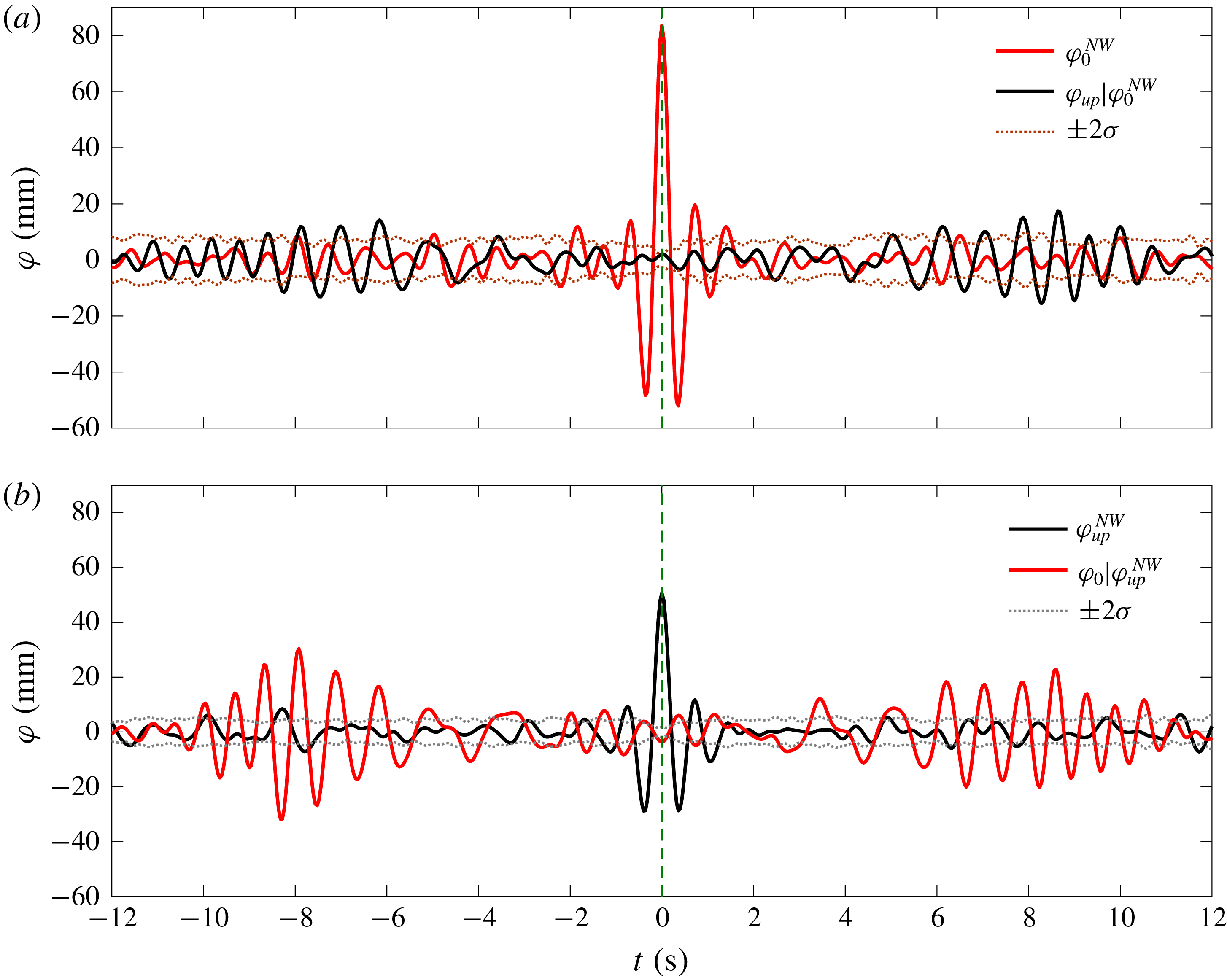
Figure 11. NewWave-type results of the response wave fields at different locations, i.e. at the ‘vessel gauge’ (
 $\unicode[STIX]{x1D711}_{0}$
) and the ‘upstream gauge’ (
$\unicode[STIX]{x1D711}_{0}$
) and the ‘upstream gauge’ (
 $\unicode[STIX]{x1D711}_{up}$
). (a) The NewResponse profile at the ‘vessel gauge’ (
$\unicode[STIX]{x1D711}_{up}$
). (a) The NewResponse profile at the ‘vessel gauge’ (
 $\unicode[STIX]{x1D711}_{0}^{NW}$
) and the associated response wave fields at the ‘upstream gauge’ (
$\unicode[STIX]{x1D711}_{0}^{NW}$
) and the associated response wave fields at the ‘upstream gauge’ (
 $\unicode[STIX]{x1D711}_{up}|\unicode[STIX]{x1D711}_{0}^{NW}$
), (b) the other way around.
$\unicode[STIX]{x1D711}_{up}|\unicode[STIX]{x1D711}_{0}^{NW}$
), (b) the other way around.

Figure 12. Reciprocity of the response wave fields at the ‘upstream gauge’
 $\unicode[STIX]{x1D711}_{up}|\unicode[STIX]{x1D711}_{0}^{NW}$
(time reversed about
$\unicode[STIX]{x1D711}_{up}|\unicode[STIX]{x1D711}_{0}^{NW}$
(time reversed about
 $t=0$
and thus ‘
$t=0$
and thus ‘
 $\pm t$
’ used here) and the ‘vessel gauge’
$\pm t$
’ used here) and the ‘vessel gauge’
 $\unicode[STIX]{x1D711}_{0}|\unicode[STIX]{x1D711}_{up}^{NW}$
;
$\unicode[STIX]{x1D711}_{0}|\unicode[STIX]{x1D711}_{up}^{NW}$
;
 $\unicode[STIX]{x1D709}_{b}=\text{r.m.s.}(\unicode[STIX]{x1D711}_{0})/\text{r.m.s.}(\unicode[STIX]{x1D711}_{up})=1.53$
.
$\unicode[STIX]{x1D709}_{b}=\text{r.m.s.}(\unicode[STIX]{x1D711}_{0})/\text{r.m.s.}(\unicode[STIX]{x1D711}_{up})=1.53$
.
Figure 11 presents the results, with (a) being the NewResponse profile at the ‘vessel gauge’ (
 $\unicode[STIX]{x1D711}_{0}^{NW}$
) and the associated response wave fields at the ‘upstream gauge’ (
$\unicode[STIX]{x1D711}_{0}^{NW}$
) and the associated response wave fields at the ‘upstream gauge’ (
 $\unicode[STIX]{x1D711}_{up}|\unicode[STIX]{x1D711}_{0}^{NW}$
) and (b) the NewResponse profile at the ‘upstream gauge’ (
$\unicode[STIX]{x1D711}_{up}|\unicode[STIX]{x1D711}_{0}^{NW}$
) and (b) the NewResponse profile at the ‘upstream gauge’ (
 $\unicode[STIX]{x1D711}_{up}^{NW}$
) and the associated response wave fields at the ‘vessel gauge’ (
$\unicode[STIX]{x1D711}_{up}^{NW}$
) and the associated response wave fields at the ‘vessel gauge’ (
 $\unicode[STIX]{x1D711}_{0}|\unicode[STIX]{x1D711}_{up}^{NW}$
). Each NewResponse is defined as the linearized average shape of the top
$\unicode[STIX]{x1D711}_{0}|\unicode[STIX]{x1D711}_{up}^{NW}$
). Each NewResponse is defined as the linearized average shape of the top
 $N$
responses as previously. One can clearly see that the NewResponse amplitude reduces from
$N$
responses as previously. One can clearly see that the NewResponse amplitude reduces from
 ${\sim}$
80 mm at the ‘vessel gauge’ to
${\sim}$
80 mm at the ‘vessel gauge’ to
 ${\sim}$
50 mm for that at the ‘upstream gauge’. We plot the time histories of
${\sim}$
50 mm for that at the ‘upstream gauge’. We plot the time histories of
 $\unicode[STIX]{x1D711}_{up}|\unicode[STIX]{x1D711}_{0}^{NW}$
and
$\unicode[STIX]{x1D711}_{up}|\unicode[STIX]{x1D711}_{0}^{NW}$
and
 $\unicode[STIX]{x1D711}_{0}|\unicode[STIX]{x1D711}_{up}^{NW}$
in figure 12, with the former being mirrored with respect to
$\unicode[STIX]{x1D711}_{0}|\unicode[STIX]{x1D711}_{up}^{NW}$
in figure 12, with the former being mirrored with respect to
 $t=0$
and scaled by a coefficient of
$t=0$
and scaled by a coefficient of
 $\unicode[STIX]{x1D709}_{b}=1.53$
. Again, we obtain a good reciprocity result between the signals. This suggests that the waves propagate from the ‘upstream gauge’ towards the structure as locally linear (first harmonic) quantities in random waves, providing further evidence of the Molin lensing phenomenon from a spatial evolution analysis.
$\unicode[STIX]{x1D709}_{b}=1.53$
. Again, we obtain a good reciprocity result between the signals. This suggests that the waves propagate from the ‘upstream gauge’ towards the structure as locally linear (first harmonic) quantities in random waves, providing further evidence of the Molin lensing phenomenon from a spatial evolution analysis.
6 Conclusions
It has been 15 years since the first study of the large wave run-up phenomena for a fixed vertical plate in regular waves (Molin et al. Reference Molin, Remy, Kimmoun and Ferrant2003). Surprisingly, very limited follow-up work has been performed, other than a comprehensive review of the work in this area by Molin’s group (Molin et al. Reference Molin, Kimmoun, Remy and Chatjigeorgiou2014). The mechanism driving the significant enhancement of wave run-up (Molin et al. Reference Molin, Remy, Kimmoun and Ferrant2003, Reference Molin, Remy, Kimmoun and Jamois2005, Reference Molin, Kimmoun, Liu, Remy and Bingham2010) is proposed to be the tertiary wave interactions of Longuet-Higgins & Phillips (Reference Longuet-Higgins and Phillips1962). Following Molin et al.’s pioneering work, we provide experimental evidence of large wave interactions on the weather side of a fixed box in random waves. Regular wave tests are also carried out in this study for a fixed rectangular box. Similar wave run-up amplifications as in Molin et al. for a fixed vertical plate have been observed, confirming that our experimental set-up is appropriate.
Using a NewWave-type analysis, we have identified both the time delay for large events and large wave run-up amplification in a random sea. The most striking effect is that the wave surface elevation in front of the fixed box can reach up to
 $4\times$
the amplitude of the incident waves at high frequencies in a broad-banded sea state. We see no significant tank resonant modes or standing waves between the wave paddles and the fixed model. We believe we have provided sufficient evidence that the significant wave surface amplification observed in our irregular wave test is also the result of tertiary wave interactions, the same mechanism as in Molin et al. (Reference Molin, Remy, Kimmoun and Jamois2005) for regular waves.
$4\times$
the amplitude of the incident waves at high frequencies in a broad-banded sea state. We see no significant tank resonant modes or standing waves between the wave paddles and the fixed model. We believe we have provided sufficient evidence that the significant wave surface amplification observed in our irregular wave test is also the result of tertiary wave interactions, the same mechanism as in Molin et al. (Reference Molin, Remy, Kimmoun and Jamois2005) for regular waves.
Such run-up amplification by tertiary wave interactions in irregular waves has not been previously reported. This effect may be of practical importance, e.g. survival of disabled floating structures and vessels in beam seas, air gap for multi-column offshore structures, breakwaters, etc.
In the present study, we have been focusing on the tertiary interactions in uni-directional waves with normal incidence. It will be also of interest to explore the role of directional spreading in the incident waves and the effect of the heading of the structure.
Acknowledgements
This work was funded by research and development grants from the University of Western Australia (UWA) and the ARC Industrial Transformation Research Hub for Offshore Floating Facilities which is funded by the Australian Research Council, Woodside Energy, Shell, Bureau Veritas and Lloyd’s Register (Grant No. IH140100012). The experiments were conducted in the Deepwater Wave Basin at Shanghai Jiao Tong University. The authors would like to thank Professor B. Molin for helpful discussions and his comments on a draft of this paper.
Appendix A
We have provided a variety of analyses in the context to support our observation of the tertiary interactions in irregular waves. However there might be concerns of some other unwanted effects contributing to the large wave run-up phenomena, e.g. ‘transverse’ tank resonance effects.

Figure 13. RAOs at the side (‘side gauge’) of the structure obtained from numerical simulations and experiments based on the steady-state time histories (from
 $t=130$
s onwards).
$t=130$
s onwards).
To eliminate the concerns, we run DIFFRACT (Sun et al. Reference Sun, Eatock Taylor and Taylor2015) providing linear diffraction predictions of the free-surface RAOs at the ‘side gauge’, 5.041 m away from the side of the fixed structure. These are compared to the RAOs obtained from the experiments in figure 13. In the linear diffraction predictions we did not take into account any tank resonance effect, or any Molin-type tertiary wave interaction effects. Therefore, the good agreement between the linear diffraction predictions and the measured data suggests that no significant tank resonance occurred in the experiments. Given the large size of the wave basin and the large distance, there will not be significant standing wave energy trapped between the wave paddles and the model. Otherwise, the ‘side gauge’ would have ‘felt’ it.

Figure 14. Illustration of NewWave-type analysis with a conditioning process. ‘C’ and ‘T’ represent crests and troughs, respectively;
 $\unicode[STIX]{x1D702}^{NW}$
refers to the NewWave profiles of the undisturbed waves (
$\unicode[STIX]{x1D702}^{NW}$
refers to the NewWave profiles of the undisturbed waves (
 $\unicode[STIX]{x1D702}$
), and
$\unicode[STIX]{x1D702}$
), and
 $\unicode[STIX]{x1D711}|\unicode[STIX]{x1D702}^{NW}$
the associated response wave profiles conditioned on the NewWave of the incident waves. Hence, for
$\unicode[STIX]{x1D711}|\unicode[STIX]{x1D702}^{NW}$
the associated response wave profiles conditioned on the NewWave of the incident waves. Hence, for
 $\unicode[STIX]{x1D711}|\unicode[STIX]{x1D702}_{(0)}$
, we find the local average shape of the response waves (
$\unicode[STIX]{x1D711}|\unicode[STIX]{x1D702}_{(0)}$
, we find the local average shape of the response waves (
 $\unicode[STIX]{x1D711}$
) around the time at which the undisturbed wave has a large crest. The subscripts ‘0’, ‘90’, ‘180’ and ‘270’ refer to the phase, and ‘1’, ‘
$\unicode[STIX]{x1D711}$
) around the time at which the undisturbed wave has a large crest. The subscripts ‘0’, ‘90’, ‘180’ and ‘270’ refer to the phase, and ‘1’, ‘
 $2+$
’, ‘
$2+$
’, ‘
 $3+$
’ and ‘
$3+$
’ and ‘
 $4+$
’ the first four harmonics extracted from the four-phase signals.
$4+$
’ the first four harmonics extracted from the four-phase signals.
Appendix B
The NewWave-type analysis requires extraction of NewWave-type profiles from the random sea signals. In this study, a set of NewWave-type profiles with four different phases are extracted, which further allow for the separation of the first four harmonics. The relationship between the undisturbed wave fields and the associated response wave fields can be then identified through a conditioning process. To provide a clear explanation of the NewWave-type analysis and the conditioning process, we summarize the procedure in the flowchart in figure 14. All the necessary signal processing was performed in MATLAB.


