


1. Introduction
Internal flows past flexible surfaces are important in the context of physiological flows and microfluidic applications, where flows are bounded by soft materials such as tissue or elastomers. The laminar–turbulent transition is of importance because both the drag force and the mixing rates are significantly higher in turbulent flows in comparison to laminar flows. An increase or decrease in the transition Reynolds number could affect the energy requirements and mixing rates in biological and microfluidic applications. Slow cross-stream mixing in microfluidic devices poses a technological barrier to the effective utilisation of lab-on-a-chip technologies (de Mello Reference de Mello2006; Whitesides Reference Whitesides2006). Due to the small dimension and flow velocity, the flow is laminar, and mixing takes place by molecular diffusion. Numerous novel methods have been proposed for enhancing the mixing rates, both passive (patterning grooves in channel walls (Stroock et al. Reference Stroock, Dertinger, Ajdari, Mezic, Stone and Whitesides2002), multiple bends (Liu et al. Reference Liu, Stremler, Sharp, Olsen, Santiago, Adrian, Aref and Beebe2000; Jiang et al. Reference Jiang, Drese, Hardt, Kupper and Schonfeld2004; Kane et al. Reference Kane, Hoffmann, Baumgartel, Seckler, Reichardt, Horsley, Schuler and Bakajin2008)) and active (ultrasound actuation (Ahmed et al. Reference Ahmed, Mao, Shi, Juluri and Huang2009), microstirrers (Mensing et al. Reference Mensing, Pearce, Graham and Beebe2004)). However, each of these has its disadvantages, such as an increase in pressure drop in grooved and bent channels and the requirement of expensive microfabrication in active strategies.
The diffusion coefficients of liquids comprising small molecules are of the order of
 $10^{-9}~\text{m}^{2}~\text{s}^{-1}$
, and the contact time required for mixing liquids across 1 mm (a typical channel width) is of the order or 1000 s. Mixing of multiple fluid streams in microfluidic devices is usually accomplished using long channels with lengths of many tens of centimetres required for a contact time of a few hundreds of seconds; these channels are curved in order to fit onto small microfluidic chips (van Berkel et al.
Reference van Berkel, Gwyer, Deane, Green, Holloway, Hollisb and Morgan2011; Han et al.
Reference Han, van Berkel, Gwyer, Capretto and Morgan2012). Due to the long path lengths and the small channel widths, large pressure drops of the order of atmospheres are required to drive the flow, and this requires pumps and compressors to be integrated into the device. This slow mixing presents a technological bottleneck to the integration of sample preparation strategies in microfluidic devices (de Mello Reference de Mello2006; Whitesides Reference Whitesides2006). Recent experiments (Verma & Kumaran Reference Verma and Kumaran2013) have demonstrated that the laminar flow in a microchannel can be destabilised at a Reynolds number much lower than the transition Reynolds number for the flow in a rigid channel if one of the walls is made sufficiently soft. The flow after transition also exhibits ultra-fast mixing and a reduction in the mixing time of up to five orders of magnitude in comparison to laminar diffusion. The flow velocities, of the order of
$10^{-9}~\text{m}^{2}~\text{s}^{-1}$
, and the contact time required for mixing liquids across 1 mm (a typical channel width) is of the order or 1000 s. Mixing of multiple fluid streams in microfluidic devices is usually accomplished using long channels with lengths of many tens of centimetres required for a contact time of a few hundreds of seconds; these channels are curved in order to fit onto small microfluidic chips (van Berkel et al.
Reference van Berkel, Gwyer, Deane, Green, Holloway, Hollisb and Morgan2011; Han et al.
Reference Han, van Berkel, Gwyer, Capretto and Morgan2012). Due to the long path lengths and the small channel widths, large pressure drops of the order of atmospheres are required to drive the flow, and this requires pumps and compressors to be integrated into the device. This slow mixing presents a technological bottleneck to the integration of sample preparation strategies in microfluidic devices (de Mello Reference de Mello2006; Whitesides Reference Whitesides2006). Recent experiments (Verma & Kumaran Reference Verma and Kumaran2013) have demonstrated that the laminar flow in a microchannel can be destabilised at a Reynolds number much lower than the transition Reynolds number for the flow in a rigid channel if one of the walls is made sufficiently soft. The flow after transition also exhibits ultra-fast mixing and a reduction in the mixing time of up to five orders of magnitude in comparison to laminar diffusion. The flow velocities, of the order of
 $1~\text{m}~\text{s}^{-1}$
, are significantly higher than those for conventional microfluidic devices. However, mixing is completed within a path length of the order of 2–3 cm (in contrast to the tens of centimetres required for conventional microfluidic devices). In addition, there is a significant deformation of the soft wall due to the applied pressure gradient (Gervais et al.
Reference Gervais, El-Ali, Guntherb and Jensen2006; Ozsun, Yakhot & Ekinci Reference Ozsun, Yakhot and Ekinci2013). A combination of the small path length and the channel deformation results in a pressure drop of less than 10 kPa, which is significantly smaller than the pressure drop of hundreds of kPa required in microfluidic devices based on laminar mixing, even though the flow rates are significantly higher. This fast mixing significantly enhances the feasibility of incorporating sample preparation steps into microfluidic devices. However, in order to facilitate design, it is necessary to have an accurate characterisation of the nature of the flow after transition. An experimental investigation of the mean and fluctuating velocities in a soft-walled microchannel after transition is the subject of the present study.
$1~\text{m}~\text{s}^{-1}$
, are significantly higher than those for conventional microfluidic devices. However, mixing is completed within a path length of the order of 2–3 cm (in contrast to the tens of centimetres required for conventional microfluidic devices). In addition, there is a significant deformation of the soft wall due to the applied pressure gradient (Gervais et al.
Reference Gervais, El-Ali, Guntherb and Jensen2006; Ozsun, Yakhot & Ekinci Reference Ozsun, Yakhot and Ekinci2013). A combination of the small path length and the channel deformation results in a pressure drop of less than 10 kPa, which is significantly smaller than the pressure drop of hundreds of kPa required in microfluidic devices based on laminar mixing, even though the flow rates are significantly higher. This fast mixing significantly enhances the feasibility of incorporating sample preparation steps into microfluidic devices. However, in order to facilitate design, it is necessary to have an accurate characterisation of the nature of the flow after transition. An experimental investigation of the mean and fluctuating velocities in a soft-walled microchannel after transition is the subject of the present study.
The flow in collapsible tubes is one of the widely studied internal flow models for the flow in airways. Here, there is a turbulent flow through an elastic tube with a constant external pressure. An increase in the flow rate within the tube can result in a decrease in the pressure, which leads to oscillations and collapse of the tube. These flows have been studied using low-dimensional models involving equations for the mass and the streamwise momentum averaged across the cross-section, along with an equation that relates the difference in the inside and outside pressures to the cross-sectional area (Shapiro Reference Shapiro1977; Cancelli & Pedley Reference Cancelli and Pedley1985; Jensen & Pedley Reference Jensen and Pedley1989; Pihler-Puzovic & Pedley Reference Pihler-Puzovic and Pedley2013). These models predict several interesting dynamical features such as tube collapse and steady flow in a collapsed tube (Jensen & Pedley Reference Jensen and Pedley1989), and self-excited and chaotic oscillations (Jensen & Heil Reference Jensen and Heil2003). Many of these features have been observed in experiments on collapsible tubes (Bertram Reference Bertram1986; Bertram, Raymond & Pedley Reference Bertram, Raymond and Pedley1991). In relation to the flow instability and transition problems discussed next, the work on flow through collapsible tubes considers flows that are generally already turbulent, and utilises approximate models which involve the mass and momentum equations coupled with an equation for the dependence of the cross-sectional area on the transmural pressure. The effect of laminar–turbulent transition on the tube collapse is an interesting aspect which does not seem to have received attention.
The pioneering experimental studies of Lahav, Eliezer & Silberberg (Reference Lahav, Eliezer and Silberberg1973) and Krindel & Silberberg (Reference Krindel and Silberberg1979) indicated that there could be a reduction in the transition Reynolds number in the flow through a tube if the wall of the tube was made of a soft polymer gel. A subsequent study (Yang, Grattoni & Zimmerman Reference Yang, Grattoni, Muggeridge and Zimmerman2000) suggested that the increase in the friction factor could be adequately explained without postulating a transition, but by just incorporating the change in tube shape due to the applied pressure gradient. However, the study of Krindel & Silberberg (Reference Krindel and Silberberg1979) was the first to suggest that there could be a decrease in the transition Reynolds number due to wall flexibility in parameter regimes of relevance to biological systems. The observation of Krindel & Silberberg (Reference Krindel and Silberberg1979) motivated a series of linear stability studies on the flow past viscoelastic surfaces (Kumaran Reference Kumaran2000, Reference Kumaran, Carpenter and Pedley2003). It should be noted that the transition Reynolds number in rigid tubes and channels is not accessible by linear stability studies, because the transition is highly subcritical and three-dimensional. In a rigid channel, linear stability analysis predicts that the flow becomes unstable at a Reynolds number of 5771 due to the Tollmien–Schlichting instability (Drazin & Reid Reference Drazin and Reid1981), whereas in experiments the transition is observed at a Reynolds number of approximately 1200 (Patel & Head Reference Patel and Head1969). Linear stability studies show that the flow through a rigid tube is stable at all Reynolds numbers, even though transition is experimentally observed at a Reynolds number of approximately 2100. For the flow in a conduit with soft viscoelastic walls, linear stability studies have shown that the flow can become unstable at a Reynolds number lower than the transition Reynolds number in a rigid conduit, provided that the wall is sufficiently soft. The transition in the flow through a soft conduit is qualitatively different from that in a rigid conduit in two important respects. First, the destabilisation is due to a coupling between the fluid velocity fluctuations and displacement fluctuations in the wall material, and the mechanism of destabilisation is the transfer of energy from the mean flow to the fluctuations due to the shear work done at the fluid–solid interface (in contrast to the Tollmien–Schlichting mechanism in the flow through hard-walled conduits). Second, linear stability analysis is found to accurately predict the transition Reynolds number observed in experiments.
For a soft-wall instability, the transition Reynolds number
 $Re_{t}=({\it\rho}VR/{\it\eta})$
is a function of the dimensionless parameter
$Re_{t}=({\it\rho}VR/{\it\eta})$
is a function of the dimensionless parameter
 ${\it\Sigma}=({\it\rho}GR^{2}/{\it\eta}^{2})$
and the viscosity ratio
${\it\Sigma}=({\it\rho}GR^{2}/{\it\eta}^{2})$
and the viscosity ratio
 ${\it\eta}_{r}=({\it\eta}_{g}/{\it\eta})$
, where
${\it\eta}_{r}=({\it\eta}_{g}/{\it\eta})$
, where
 ${\it\rho}$
and
${\it\rho}$
and
 ${\it\eta}$
are the fluid density and viscosity,
${\it\eta}$
are the fluid density and viscosity,
 $G$
and
$G$
and
 ${\it\eta}_{g}$
are the shear modulus and viscosity of the viscoelastic wall,
${\it\eta}_{g}$
are the shear modulus and viscosity of the viscoelastic wall,
 $R$
is the characteristic flow length scale and
$R$
is the characteristic flow length scale and
 $V$
is the characteristic velocity. There is an instability even in the limit of zero Reynolds number when the parameter
$V$
is the characteristic velocity. There is an instability even in the limit of zero Reynolds number when the parameter
 $V{\it\eta}/GR$
exceeds a critical value (Kumaran, Fredrickson & Pincus Reference Kumaran, Fredrickson and Pincus1994; Kumaran Reference Kumaran1995). The specific wall model does have a significant effect on the zero-Reynolds-number transition (Thaokar, Shankar & Kumaran Reference Thaokar, Shankar and Kumaran2001; Gkanis & Kumar Reference Gkanis and Kumar2005; Chokshi & Kumaran Reference Chokshi and Kumaran2008; Gaurav & Shankar Reference Shankar2009), and this transition is shown to be subcritical by weakly nonlinear stability analyses (Shankar & Kumaran Reference Shankar and Kumaran2001b
; Chokshi & Kumaran Reference Chokshi and Kumaran2007). Other mechanisms of instability at high Reynolds number are also qualitatively different from the instability for the flow past a rigid surface. Viscous effects are negligible in the bulk of the flow in the high-Reynolds-number ‘inviscid’ instability (Kumaran Reference Kumaran1996; Shankar & Kumaran Reference Shankar and Kumaran1999, Reference Shankar and Kumaran2000), though they are significant in boundary layers of thickness
$V{\it\eta}/GR$
exceeds a critical value (Kumaran, Fredrickson & Pincus Reference Kumaran, Fredrickson and Pincus1994; Kumaran Reference Kumaran1995). The specific wall model does have a significant effect on the zero-Reynolds-number transition (Thaokar, Shankar & Kumaran Reference Thaokar, Shankar and Kumaran2001; Gkanis & Kumar Reference Gkanis and Kumar2005; Chokshi & Kumaran Reference Chokshi and Kumaran2008; Gaurav & Shankar Reference Shankar2009), and this transition is shown to be subcritical by weakly nonlinear stability analyses (Shankar & Kumaran Reference Shankar and Kumaran2001b
; Chokshi & Kumaran Reference Chokshi and Kumaran2007). Other mechanisms of instability at high Reynolds number are also qualitatively different from the instability for the flow past a rigid surface. Viscous effects are negligible in the bulk of the flow in the high-Reynolds-number ‘inviscid’ instability (Kumaran Reference Kumaran1996; Shankar & Kumaran Reference Shankar and Kumaran1999, Reference Shankar and Kumaran2000), though they are significant in boundary layers of thickness
 $Re^{-1/2}$
at the walls. Similarly to the Tollmien–Schlichting mechanism, there is an internal critical layer of thickness
$Re^{-1/2}$
at the walls. Similarly to the Tollmien–Schlichting mechanism, there is an internal critical layer of thickness
 $Re^{-1/3}$
within the flow where the wave speed is equal to the flow velocity. The transition Reynolds number follows the scaling
$Re^{-1/3}$
within the flow where the wave speed is equal to the flow velocity. The transition Reynolds number follows the scaling
 $Re_{t}\propto {\it\Sigma}^{1/2}$
. The destabilising mechanism in the ‘wall mode’ instability at high Reynolds numbers (Kumaran Reference Kumaran1998; Shankar & Kumaran Reference Shankar and Kumaran2001a
, Reference Shankar and Kumaran2002) is the transfer of energy from the mean flow to the fluctuations due to the shear work at the interface. The viscous stress perturbations are important in a wall layer of thickness
$Re_{t}\propto {\it\Sigma}^{1/2}$
. The destabilising mechanism in the ‘wall mode’ instability at high Reynolds numbers (Kumaran Reference Kumaran1998; Shankar & Kumaran Reference Shankar and Kumaran2001a
, Reference Shankar and Kumaran2002) is the transfer of energy from the mean flow to the fluctuations due to the shear work at the interface. The viscous stress perturbations are important in a wall layer of thickness
 $Re^{-1/3}$
at the wall, and the transition Reynolds number scales as
$Re^{-1/3}$
at the wall, and the transition Reynolds number scales as
 $Re_{t}\propto {\it\Sigma}^{3/4}$
. Weakly nonlinear studies indicate that this instability is supercritical (Chokshi & Kumaran Reference Chokshi and Kumaran2009).
$Re_{t}\propto {\it\Sigma}^{3/4}$
. Weakly nonlinear studies indicate that this instability is supercritical (Chokshi & Kumaran Reference Chokshi and Kumaran2009).
The viscous instability has been verified in experiments (Kumaran & Muralikrishnan Reference Kumaran and Muralikrishnan2000; Muralikrishnan & Kumaran Reference Muralikrishnan and Kumaran2002; Eggert & Kumar Reference Eggert and Kumar2004), where a Couette flow was set up in a commercial rheometer between a soft polyacrylamide gel as the bottom surface and a rotating top plate, and a viscous silicone oil (with viscosity
 $10^{3}$
times that of water) was sheared in the gap between the two surfaces. The transition value of
$10^{3}$
times that of water) was sheared in the gap between the two surfaces. The transition value of
 $(V{\it\eta}/GR)$
for the destabilisation of the viscous modes is in quantitative agreement with theoretical predictions, and experiments also confirmed that the bifurcation is subcritical. Thus, the low-Reynolds-number instability phenomenon is now well understood both in theory and in experiments. In contrast, the practical realisation of the high-Reynolds-number instability was not considered feasible for a some time after the theory was formulated. In tubes and channels, the transition Reynolds number for the inviscid and wall mode instability is lower than that for transition in a rigid conduit only for low values of the parameter
$(V{\it\eta}/GR)$
for the destabilisation of the viscous modes is in quantitative agreement with theoretical predictions, and experiments also confirmed that the bifurcation is subcritical. Thus, the low-Reynolds-number instability phenomenon is now well understood both in theory and in experiments. In contrast, the practical realisation of the high-Reynolds-number instability was not considered feasible for a some time after the theory was formulated. In tubes and channels, the transition Reynolds number for the inviscid and wall mode instability is lower than that for transition in a rigid conduit only for low values of the parameter
 ${\it\Sigma}$
, which requires a small characteristic dimension (1 mm or less) and unrealistically low shear modulus
${\it\Sigma}$
, which requires a small characteristic dimension (1 mm or less) and unrealistically low shear modulus
 $G$
of a few tens of pascals. In soft solids such as polymer gels, the lowest feasible shear modulus is of the order of a few thousands of pascals. For such solids, the transition Reynolds number for the wall mode and inviscid mode instabilities is higher than the transition Reynolds number in a rigid conduit even for characteristic dimension
$G$
of a few tens of pascals. In soft solids such as polymer gels, the lowest feasible shear modulus is of the order of a few thousands of pascals. For such solids, the transition Reynolds number for the wall mode and inviscid mode instabilities is higher than the transition Reynolds number in a rigid conduit even for characteristic dimension
 $100~{\rm\mu}\text{m}$
to 1 mm. The value of
$100~{\rm\mu}\text{m}$
to 1 mm. The value of
 ${\it\Sigma}$
could be reduced by decreasing the characteristic dimensions of the conduit to tens of microns or less or using fluids of very high viscosity, but this would require a very large pressure difference to generate the velocity required for transition; such high pressure differences on conduits of small dimensions are likely to result in mechanical failure.
${\it\Sigma}$
could be reduced by decreasing the characteristic dimensions of the conduit to tens of microns or less or using fluids of very high viscosity, but this would require a very large pressure difference to generate the velocity required for transition; such high pressure differences on conduits of small dimensions are likely to result in mechanical failure.
Recent experiments (Verma & Kumaran Reference Verma and Kumaran2012, Reference Verma and Kumaran2013, Reference Verma and Kumaran2015) have shown that the high-Reynolds-number instability can be practically realised at a Reynolds number as low as 500 in tubes of diameter approximately 1 mm and length approximately 10 cm if the wall is made sufficiently soft, and at a minimum Reynolds number of 200 in a microchannel of length 3 cm, width (spanwise direction) approximately 1.5 mm and height
 $100~{\rm\mu}\text{m}$
if one of the walls is made sufficiently soft. The flow instability was found to be accompanied by the onset of wall motion. Different techniques were used for observing the instability of the laminar flow. In the dye-stream method, a dye is introduced at the centre, and the breakup of the dye is an indicator of the instability. The pressure difference across a deformed channel or tube was also compared with the computed prediction for the laminar flow in a channel or tube of the same shape using a finite difference scheme, and transition was inferred when the theoretical prediction was significantly lower than the experimental result, indicating that the flow had transitioned from a laminar to a more complicated velocity profile. In order to detect wall oscillations, fluorescent microbeads were embedded in the soft wall, and the motion of the beads was analysed using laser scattering. All three experimental measurements indicated that a flow instability and a transition to a non-laminar velocity profile occur simultaneously with the onset of wall motion. In both tubes and microchannels, the instability was observed at a Reynolds number smaller, by a factor of approximately 10, than that predicted theoretically for a parabolic flow in a channel or tube with a constant pressure gradient (Gaurav & Shankar Reference Shankar2009, Reference Shankar2010). A linear stability analysis indicated that the flow stability is significantly affected by wall deformation due to the applied pressure gradient. There is an expansion of the conduit close to the inlet, and then a contraction further downstream. This results in a modification of the velocity profile, and the pressure gradient is not a constant in the flow direction. When the modification of the pressure gradient and the velocity profile due to wall deformation is incorporated in the analysis, the predicted transition Reynolds number is in quantitative agreement with experimental results (Verma & Kumaran Reference Verma and Kumaran2013, Reference Verma and Kumaran2015). Linear stability analysis also predicts that the instability first occurs in the downstream converging section of the conduit, and not in the upstream diverging section; this is also in agreement with experimental observations.
$100~{\rm\mu}\text{m}$
if one of the walls is made sufficiently soft. The flow instability was found to be accompanied by the onset of wall motion. Different techniques were used for observing the instability of the laminar flow. In the dye-stream method, a dye is introduced at the centre, and the breakup of the dye is an indicator of the instability. The pressure difference across a deformed channel or tube was also compared with the computed prediction for the laminar flow in a channel or tube of the same shape using a finite difference scheme, and transition was inferred when the theoretical prediction was significantly lower than the experimental result, indicating that the flow had transitioned from a laminar to a more complicated velocity profile. In order to detect wall oscillations, fluorescent microbeads were embedded in the soft wall, and the motion of the beads was analysed using laser scattering. All three experimental measurements indicated that a flow instability and a transition to a non-laminar velocity profile occur simultaneously with the onset of wall motion. In both tubes and microchannels, the instability was observed at a Reynolds number smaller, by a factor of approximately 10, than that predicted theoretically for a parabolic flow in a channel or tube with a constant pressure gradient (Gaurav & Shankar Reference Shankar2009, Reference Shankar2010). A linear stability analysis indicated that the flow stability is significantly affected by wall deformation due to the applied pressure gradient. There is an expansion of the conduit close to the inlet, and then a contraction further downstream. This results in a modification of the velocity profile, and the pressure gradient is not a constant in the flow direction. When the modification of the pressure gradient and the velocity profile due to wall deformation is incorporated in the analysis, the predicted transition Reynolds number is in quantitative agreement with experimental results (Verma & Kumaran Reference Verma and Kumaran2013, Reference Verma and Kumaran2015). Linear stability analysis also predicts that the instability first occurs in the downstream converging section of the conduit, and not in the upstream diverging section; this is also in agreement with experimental observations.
Large velocity fluctuations in the spanwise direction were observed after transition in the microchannel experiments of Verma & Kumaran (Reference Verma and Kumaran2013) in microchannels of length approximately 3 cm. These fluctuations resulted in ultra-fast mixing between two streams that were introduced side-by-side in the microchannel. Mixing was characterised in two ways. The first was by pumping in two fluid streams of different colour through two adjacent inlets, and visually characterising the mixing by image analysis. The second was by separating out the two inlet streams at the outlet in a symmetric manner, and using conductivity measurements to determine the extent of mixing. These measurements indicated that the time required for complete mixing, which is a few tens of milliseconds, is lower, by five orders of magnitude, in comparison to the time required for molecular diffusion in a laminar flow across a distance of approximately 1 mm. This rapid mixing was accompanied by a relatively small increase in the pressure difference required to drive the flow, because the channel expansion due to the pressure difference results in a higher cross-sectional area and lower flow resistance.
It is important to reiterate that the mechanism of destabilisation, which involves a coupling between fluid and wall dynamics, is qualitatively different from that for transition in a rigid channel, and all of the available evidence indicates that the transition is accurately predicted by a linear stability analysis. A critical gap in our current understanding is the nature of the flow after transition. Experiments do show large velocity fluctuations in the spanwise direction along the width of the microchannel after transition, indicating that the flow is three-dimensional. However, there are no direct velocity measurements in the direction perpendicular to the soft wall across the smallest dimension of the channel, in which the mean velocity gradient is the largest. The objective of this paper is to examine the nature of the flow after the instability of the laminar flow. Dye-stream experiments were carried out by Verma & Kumaran (Reference Verma and Kumaran2013), where they introduced a dye at the centre of the channel and visualised the progression of the dye downstream. In these experiments, regular patterns were not observed, but there was a catastrophic breakup of the dye stream at transition. This motivates us to examine whether the flow transition exhibits the features of turbulence, by comparing the flow features with those of turbulence in rigid channels.
Here, we study the nature of the velocity profile in the case where the transition is induced by a dynamical interaction between the fluid and a soft wall when the flow length scale is of the order of
 $200{-}300~{\rm\mu}\text{m}$
. Since transition occurs at a Reynolds number of approximately 250 for the softest gels used here, the nature of the flow after transition is compared with turbulent flows in rigid channels at much higher Reynolds numbers. Of interest are the magnitudes of the velocity fluctuations (when scaled by the maximum velocity or friction velocity), as well as the shape of the profiles of the mean velocity (specifically the presence of the viscous sublayer, buffer layer and logarithmic layer), the root mean square of the fluctuating velocities (the near-wall peak in the intensity of the streamwise fluctuating velocity and the Reynolds stress profiles) and the fluctuating energy production rates. In a rigid-walled channel, all components of the fluctuating velocity decrease to zero due to the no-slip condition, and so the mean square of the fluctuating velocities, Reynolds stress and fluctuating energy production rate are zero at the wall. In a soft-walled channel, there could be wall motion due to the stresses exerted by the flow, and so there is the possibility that the mean square of the fluctuating velocities and the Reynolds stress are not zero at the wall. In addition, the mechanism of destabilisation of the laminar flow is the transfer of energy from the mean flow to the fluctuations due to the shear work done at the fluid–solid interface. If this mechanism persists after transition, there is the possibility that the fluctuating energy production is a maximum at the fluid–solid interface.
$200{-}300~{\rm\mu}\text{m}$
. Since transition occurs at a Reynolds number of approximately 250 for the softest gels used here, the nature of the flow after transition is compared with turbulent flows in rigid channels at much higher Reynolds numbers. Of interest are the magnitudes of the velocity fluctuations (when scaled by the maximum velocity or friction velocity), as well as the shape of the profiles of the mean velocity (specifically the presence of the viscous sublayer, buffer layer and logarithmic layer), the root mean square of the fluctuating velocities (the near-wall peak in the intensity of the streamwise fluctuating velocity and the Reynolds stress profiles) and the fluctuating energy production rates. In a rigid-walled channel, all components of the fluctuating velocity decrease to zero due to the no-slip condition, and so the mean square of the fluctuating velocities, Reynolds stress and fluctuating energy production rate are zero at the wall. In a soft-walled channel, there could be wall motion due to the stresses exerted by the flow, and so there is the possibility that the mean square of the fluctuating velocities and the Reynolds stress are not zero at the wall. In addition, the mechanism of destabilisation of the laminar flow is the transfer of energy from the mean flow to the fluctuations due to the shear work done at the fluid–solid interface. If this mechanism persists after transition, there is the possibility that the fluctuating energy production is a maximum at the fluid–solid interface.
There are several challenges in setting up the experiments and carrying out the experimental measurements. There is a significant deformation of the soft wall due to the pressure gradient across the channel, and so the cross-section is not rectangular in our experiments. The measurements are carried out only in the downstream section where the channel is converging and the slope of the wall is small, so that the mean flow along the central plane of the channel is close to a two-dimensional flow. However, the velocity profile is different from a parabolic profile due to the slope of the wall. Since the walls of the channel are made of polymer gels, the walls are relatively smooth; the maximum roughness (difference between maximum and minimum height) is approximately
 $0.5~{\rm\mu}\text{m}$
over an area of
$0.5~{\rm\mu}\text{m}$
over an area of
 $0.5~\text{mm}\times 0.5~\text{mm}$
for the soft wall. However, the roughness scaled by the height of the microchannel, which is approximately 0.2 %, is relatively large compared with that in large pipes and in wind tunnels where noise-free experiments on turbulence are carried out.
$0.5~\text{mm}\times 0.5~\text{mm}$
for the soft wall. However, the roughness scaled by the height of the microchannel, which is approximately 0.2 %, is relatively large compared with that in large pipes and in wind tunnels where noise-free experiments on turbulence are carried out.
Micro particle image velocimetry (Micro PIV) has been used extensively for characterising flows in microfluidic devices. In these measurements, images of the microfluidic chip are usually captured from above, resulting in velocities being averaged over the height (smallest dimension) of the microchannel. In the present experiments, it is necessary to determine the variations in the mean and fluctuating velocities along the height of the microchannel. This dimension is typically very small; in our experiments, even after the channel expands under an applied pressure gradient, the channel height (smallest dimension) is only
 $200{-}300~{\rm\mu}\text{m}$
. The seed particles used for velocity tracking need to be at most
$200{-}300~{\rm\mu}\text{m}$
. The seed particles used for velocity tracking need to be at most
 $2{-}3~{\rm\mu}\text{m}$
in diameter, smaller than the microchannel height by two orders of magnitude, for accurate velocity measurements. It is necessary to obtain a spatial resolution of the order of
$2{-}3~{\rm\mu}\text{m}$
in diameter, smaller than the microchannel height by two orders of magnitude, for accurate velocity measurements. It is necessary to obtain a spatial resolution of the order of
 $10~{\rm\mu}\text{m}$
in order to track these particles accurately. The laser sheet used in the experiments has to be sufficiently thin, much smaller than the spanwise width of the microchannel which is 1.5 mm, in order to obtain local measurements and to avoid averaging in the spanwise direction. In our experiments, the laser sheet is confined to a width of 0.2 mm at the central plane along the spanwise direction. It is also necessary to use high-speed imaging, since instability occurs when the mean velocity in the microchannel is
$10~{\rm\mu}\text{m}$
in order to track these particles accurately. The laser sheet used in the experiments has to be sufficiently thin, much smaller than the spanwise width of the microchannel which is 1.5 mm, in order to obtain local measurements and to avoid averaging in the spanwise direction. In our experiments, the laser sheet is confined to a width of 0.2 mm at the central plane along the spanwise direction. It is also necessary to use high-speed imaging, since instability occurs when the mean velocity in the microchannel is
 $1~\text{m}~\text{s}^{-1}$
or more.
$1~\text{m}~\text{s}^{-1}$
or more.
Wall motion is also difficult to measure experimentally for multiple reasons. Previous linear stability studies (Shankar & Kumaran Reference Shankar and Kumaran2001a
, Reference Shankar and Kumaran2002) indicate that for the most unstable ‘wall modes’, the normal displacement of the wall is zero in the leading approximation in an asymptotic expansion in the parameter
 $\mathit{Re}^{-1/3}$
, where
$\mathit{Re}^{-1/3}$
, where
 $\mathit{Re}$
is the Reynolds number. A weakly nonlinear analysis (Chokshi & Kumaran Reference Chokshi and Kumaran2009) found that the wall mode instability is supercritical, and the transition amplitude is typically small, of the order of
$\mathit{Re}$
is the Reynolds number. A weakly nonlinear analysis (Chokshi & Kumaran Reference Chokshi and Kumaran2009) found that the wall mode instability is supercritical, and the transition amplitude is typically small, of the order of
 $10^{-3}\sqrt{\mathit{Re }-\mathit{ Re }_{t}}$
times the channel height close to transition for the parameter values used here, where
$10^{-3}\sqrt{\mathit{Re }-\mathit{ Re }_{t}}$
times the channel height close to transition for the parameter values used here, where
 $\mathit{Re}_{t}$
is the transition Reynolds number. This would suggest that perpendicular wall motion will be of the order of microns when
$\mathit{Re}_{t}$
is the transition Reynolds number. This would suggest that perpendicular wall motion will be of the order of microns when
 $\mathit{Re}-\mathit{Re}_{t}\sim 100$
; wall displacement of such small magnitude is difficult to measure. Previous experiments (Verma & Kumaran Reference Verma and Kumaran2012, Reference Verma and Kumaran2013) found no discernible wall motion perpendicular to the interface, though wall motion parallel to the interface was inferred by laser scattering off beads embedded in the soft wall. The displacement parallel to the surface, due to the stress exerted by the fluid, is of the order of
$\mathit{Re}-\mathit{Re}_{t}\sim 100$
; wall displacement of such small magnitude is difficult to measure. Previous experiments (Verma & Kumaran Reference Verma and Kumaran2012, Reference Verma and Kumaran2013) found no discernible wall motion perpendicular to the interface, though wall motion parallel to the interface was inferred by laser scattering off beads embedded in the soft wall. The displacement parallel to the surface, due to the stress exerted by the fluid, is of the order of
 $5{-}10~{\rm\mu}\text{m}$
for the flow parameters used in the experiments, and so it is necessary to use high magnification to detect these displacements. Another issue is the time resolution required for the detection of wall motion. Linear stability studies (Shankar & Kumaran Reference Shankar and Kumaran2001a
, Reference Shankar and Kumaran2002) predict that the frequency of perturbations at transition is of the order of
$5{-}10~{\rm\mu}\text{m}$
for the flow parameters used in the experiments, and so it is necessary to use high magnification to detect these displacements. Another issue is the time resolution required for the detection of wall motion. Linear stability studies (Shankar & Kumaran Reference Shankar and Kumaran2001a
, Reference Shankar and Kumaran2002) predict that the frequency of perturbations at transition is of the order of
 $10^{4}{-}10^{5}~\text{Hz}$
. Such high frequencies are also very difficult to detect by direct imaging techniques. Here, we use direct imaging of dye-marked spots on the fluid–wall interface to detect low-frequency wall motion along the plane parallel to the fluid–wall interface, in order to determine wall displacement due to the fluid stress as well as low-frequency wall motion after transition.
$10^{4}{-}10^{5}~\text{Hz}$
. Such high frequencies are also very difficult to detect by direct imaging techniques. Here, we use direct imaging of dye-marked spots on the fluid–wall interface to detect low-frequency wall motion along the plane parallel to the fluid–wall interface, in order to determine wall displacement due to the fluid stress as well as low-frequency wall motion after transition.
The experimental methods developed and used here are discussed in § 2, and the experimental results for both the fluid velocity and the wall motion are provided in § 3. The important conclusions are discussed in § 4.
2. Experimental methods
2.1. Channel fabrication
The microchannels of height
 $160~{\rm\mu}\text{m}$
were fabricated using a modification of the procedure of Verma & Kumaran (Reference Verma and Kumaran2013). Due to limitations on the mechanical pressure that could be applied across these channels on account of the bonding strength, the maximum Reynolds number that could be attained was in the range of 400–500. It was not possible to validate the imaging and image analysis procedure for the turbulent velocity fluctuations in the microchannel with hard walls, since the transition Reynolds number of 1200 is not attainable in the microchannel. Therefore, channels with height 1.52 mm and width 1.5 cm were fabricated using a different procedure but with the same optical set-up (apart from the difference in magnification of a factor of 10) in order to validate the procedure for measuring the turbulent velocity fluctuations, as discussed in the Appendix. The experimental results for the mean velocity, the streamwise and wall-normal root mean square of the fluctuating velocities and the Reynolds stress were found to be in agreement, to within the experimental errors, with direct numerical simulation (DNS) channel flow simulations at a Reynolds number of 3500. This validates the experimental procedure for the velocity measurements discussed in § 2.4. The turbulence measurements in the Appendix, which were carried out in a rigid-walled channel, also provide a context for analysing the similarities and differences between rigid-wall turbulence and the flow after transition in the present system.
$160~{\rm\mu}\text{m}$
were fabricated using a modification of the procedure of Verma & Kumaran (Reference Verma and Kumaran2013). Due to limitations on the mechanical pressure that could be applied across these channels on account of the bonding strength, the maximum Reynolds number that could be attained was in the range of 400–500. It was not possible to validate the imaging and image analysis procedure for the turbulent velocity fluctuations in the microchannel with hard walls, since the transition Reynolds number of 1200 is not attainable in the microchannel. Therefore, channels with height 1.52 mm and width 1.5 cm were fabricated using a different procedure but with the same optical set-up (apart from the difference in magnification of a factor of 10) in order to validate the procedure for measuring the turbulent velocity fluctuations, as discussed in the Appendix. The experimental results for the mean velocity, the streamwise and wall-normal root mean square of the fluctuating velocities and the Reynolds stress were found to be in agreement, to within the experimental errors, with direct numerical simulation (DNS) channel flow simulations at a Reynolds number of 3500. This validates the experimental procedure for the velocity measurements discussed in § 2.4. The turbulence measurements in the Appendix, which were carried out in a rigid-walled channel, also provide a context for analysing the similarities and differences between rigid-wall turbulence and the flow after transition in the present system.

Figure 1. Schematics of the top views of the two different microchannel configurations used (a,b), the channel cross-section in the absence of flow (c) and the channel cross-section in the presence of flow (d), showing the deformation of the soft part. The shaded portions in (a,b) are the regions where the bottom wall is soft. The
 $y$
and
$y$
and
 $z$
coordinates for the wall-normal and spanwise directions are shown in (d).
$z$
coordinates for the wall-normal and spanwise directions are shown in (d).
The rectangular microchannels of dimensions
 $160~{\rm\mu}\text{m}$
height, 1.5 mm width and approximately 40 mm length were fabricated in cross-linked PDMS (polydimethyl-siloxane) gels (Sylgard 184 silicone elastomer kit from Dow Corning) as shown in figure 1. The channel consists of two sections, the upstream development section of length approximately 1 cm to attenuate disturbances at the inlet and a deformable test section of length approximately 3 cm where the velocities are measured. In the development section, all four walls are fabricated using 10 % cross-linker catalyst concentration, as prescribed for the Sylgard 184 kit, which results in a shear modulus of approximately 0.55 MPa. In the test section, three of the walls are made of hard PDMS of shear modulus 0.55 MPa, while the fourth wall is made of soft PDMS with a lower elasticity modulus, by decreasing the catalyst concentration during the fabrication process. Two different catalyst concentrations, 1.75 % and 2 %, were used in the experiments, and the elasticity moduli for these gels are given in table 1. Soft walls with four different shear moduli were used in the earlier study of Verma & Kumaran (Reference Verma and Kumaran2013) on the transition in a soft-walled channel of height
$160~{\rm\mu}\text{m}$
height, 1.5 mm width and approximately 40 mm length were fabricated in cross-linked PDMS (polydimethyl-siloxane) gels (Sylgard 184 silicone elastomer kit from Dow Corning) as shown in figure 1. The channel consists of two sections, the upstream development section of length approximately 1 cm to attenuate disturbances at the inlet and a deformable test section of length approximately 3 cm where the velocities are measured. In the development section, all four walls are fabricated using 10 % cross-linker catalyst concentration, as prescribed for the Sylgard 184 kit, which results in a shear modulus of approximately 0.55 MPa. In the test section, three of the walls are made of hard PDMS of shear modulus 0.55 MPa, while the fourth wall is made of soft PDMS with a lower elasticity modulus, by decreasing the catalyst concentration during the fabrication process. Two different catalyst concentrations, 1.75 % and 2 %, were used in the experiments, and the elasticity moduli for these gels are given in table 1. Soft walls with four different shear moduli were used in the earlier study of Verma & Kumaran (Reference Verma and Kumaran2013) on the transition in a soft-walled channel of height
 $160~{\rm\mu}\text{m}$
. The transition Reynolds numbers were
$160~{\rm\mu}\text{m}$
. The transition Reynolds numbers were
 $Re=250$
for the wall with shear modulus 18 kPa,
$Re=250$
for the wall with shear modulus 18 kPa,
 $Re=332$
for the wall with shear modulus 26 kPa,
$Re=332$
for the wall with shear modulus 26 kPa,
 $Re=378$
for the wall with shear modulus 37 kPa, and there was no transition for
$Re=378$
for the wall with shear modulus 37 kPa, and there was no transition for
 $Re<422$
for the wall with 54 kPa. There is an experimental limitation that the maximum Reynolds number that can be repeatedly achieved is approximately 400 before there is mechanical failure of the joints. Therefore, we were not able to observe turbulence for the soft wall with shear modulus 54 kPa. For the soft wall with shear modulus 37 kPa, the range of Reynolds numbers for which the flow is unstable, 378–400, is too small to be able to draw conclusions about the variation of the flow properties with Reynolds number. Therefore, we have studied the two lower shear moduli for which there is a sufficient range of Reynolds numbers over which the flow is turbulent.
$Re<422$
for the wall with 54 kPa. There is an experimental limitation that the maximum Reynolds number that can be repeatedly achieved is approximately 400 before there is mechanical failure of the joints. Therefore, we were not able to observe turbulence for the soft wall with shear modulus 54 kPa. For the soft wall with shear modulus 37 kPa, the range of Reynolds numbers for which the flow is unstable, 378–400, is too small to be able to draw conclusions about the variation of the flow properties with Reynolds number. Therefore, we have studied the two lower shear moduli for which there is a sufficient range of Reynolds numbers over which the flow is turbulent.
Table 1. The shear modulus
 $G$
, compression modulus
$G$
, compression modulus
 $K$
, Youngs modulus
$K$
, Youngs modulus
 $E$
and Poisson ratio
$E$
and Poisson ratio
 ${\it\nu}$
for the gels with catalyst concentrations of 1.75 % and 2 % used for the soft wall.
${\it\nu}$
for the gels with catalyst concentrations of 1.75 % and 2 % used for the soft wall.
Two different designs for the channel inlet manifolds were used in the experiments. The first is the Y-inlet, whose top view is shown in figure 1(a), where the flow rates in the two inlets are equal. In this design, two different fluids can be pumped into the two different inlets, and the mixing can be visually monitored. The two inlets are arranged symmetrically with equal widths. The second design is the split inlet (figure 1 b) with a central inlet of width 0.3 mm and two outer inlets of width 0.6 mm converging to a microchannel of width 1.5 mm. This is used to inject a dye stream at the centre of the channel and observe the breakup of the dye stream when there is a transition. In this case, the flow rates in the central channel and outer channels are maintained at the ratio 1:4, so that the velocities of these individual streams are equal at the entrance to the development section. Although the velocity profile at the inlet to the development section does depend on the inlet manifold, it has been verified (Verma & Kumaran Reference Verma and Kumaran2013) that the velocity profiles downstream in the test section do not depend on the specific type of inlet used. The split inlet was used in most of the experiments conducted here.
2.2. Experimental set-up
For reference, we consider a coordinate system where the
 $x$
axis is along the length of the channel, the
$x$
axis is along the length of the channel, the
 $z$
axis is in the spanwise direction with origin at the central plane and the
$z$
axis is in the spanwise direction with origin at the central plane and the
 $y$
axis is directed vertically upward from the soft wall across the height (smallest dimension) of the channel, as shown in figure 1(d). The channel is fixed on an optical breadboard of dimensions
$y$
axis is directed vertically upward from the soft wall across the height (smallest dimension) of the channel, as shown in figure 1(d). The channel is fixed on an optical breadboard of dimensions
 $1.2~\text{m}\times 0.9~\text{m}$
mounted on a frame with levelling screws from Holmarc Opto-Mechatronics Pvt. Ltd, Kochi, which has standard M6 tapped levelling screws on a 25 mm grid. At the bottom of the mounting assembly for the microchannel is a motorised linear translation stage with a maximum of 150 mm travel, 1 mm pitch screw driven by a stepper motor with
$1.2~\text{m}\times 0.9~\text{m}$
mounted on a frame with levelling screws from Holmarc Opto-Mechatronics Pvt. Ltd, Kochi, which has standard M6 tapped levelling screws on a 25 mm grid. At the bottom of the mounting assembly for the microchannel is a motorised linear translation stage with a maximum of 150 mm travel, 1 mm pitch screw driven by a stepper motor with
 $1.8^{\circ }$
steps in the
$1.8^{\circ }$
steps in the
 $x$
(flow) direction. The motor has a programmable control unit with a maximum speed of
$x$
(flow) direction. The motor has a programmable control unit with a maximum speed of
 $3.125~\text{mm}~\text{s}^{-1}$
. Above this is fixed a manual linear translation stage with maximum travel of 25 mm in the spanwise
$3.125~\text{mm}~\text{s}^{-1}$
. Above this is fixed a manual linear translation stage with maximum travel of 25 mm in the spanwise
 $z$
direction for positioning of the microchannel. Above this are two goniometers which permit rotation of the stage by
$z$
direction for positioning of the microchannel. Above this are two goniometers which permit rotation of the stage by
 $\pm 10^{\circ }$
about the
$\pm 10^{\circ }$
about the
 $z$
and
$z$
and
 $x$
axes respectively. A plate of dimension
$x$
axes respectively. A plate of dimension
 $10~\text{cm}\times 5~\text{cm}$
is fixed on top of the goniometer, and the microchannel is taped onto the stage.
$10~\text{cm}\times 5~\text{cm}$
is fixed on top of the goniometer, and the microchannel is taped onto the stage.

Figure 2. The configuration for imaging the channel from above (a) and from the side (b).
Two different configurations are used for acquiring images of the channel. For the dye-stream and wall motion experiments, the configuration shown in figure 2(a) is used to take images in the
 $x{-}z$
plane from above the channel. A Navitar zoom tube with
$x{-}z$
plane from above the channel. A Navitar zoom tube with
 $48\times$
magnification is connected to a Motion Pro HS-4 camera with a maximum framing rate of 1000 Hz and resolution of
$48\times$
magnification is connected to a Motion Pro HS-4 camera with a maximum framing rate of 1000 Hz and resolution of
 $512\times 512~\text{pixels}$
with optical axis along the
$512\times 512~\text{pixels}$
with optical axis along the
 $y$
direction. Lighting for the channel is provided from below using an MI 150 high-intensity illuminator from Edmund Optics, where the illumination is delivered using an optic fibre cable through a hole carved at the bottom of the mounting plate. For the particle image velocimetry (PIV) measurements and for measurements of the channel deformation, the configuration shown in figure 2(b) is used. A Navitar
$y$
direction. Lighting for the channel is provided from below using an MI 150 high-intensity illuminator from Edmund Optics, where the illumination is delivered using an optic fibre cable through a hole carved at the bottom of the mounting plate. For the particle image velocimetry (PIV) measurements and for measurements of the channel deformation, the configuration shown in figure 2(b) is used. A Navitar
 $48\times$
zoom tube is attached to the camera to provide adequate magnification. The camera and zoom tube assembly for capturing the images is aligned horizontally with optical axis along the
$48\times$
zoom tube is attached to the camera to provide adequate magnification. The camera and zoom tube assembly for capturing the images is aligned horizontally with optical axis along the
 $z$
direction for capturing images of the flow from the side. In all cases, the flow is driven through the two inlets by NE-1000 (New Era) syringe pumps which are not placed on the breadboard to avoid disturbances.
$z$
direction for capturing images of the flow from the side. In all cases, the flow is driven through the two inlets by NE-1000 (New Era) syringe pumps which are not placed on the breadboard to avoid disturbances.
In the experiments, it is observed that the channel deforms in the test section when there is a pressure difference between the inlet and the outlet (Gervais et al.
Reference Gervais, El-Ali, Guntherb and Jensen2006; Ozsun et al.
Reference Ozsun, Yakhot and Ekinci2013). This wall deformation significantly affects even the laminar velocity profile, and so it is important to characterise this accurately. Since the top and sidewalls are rigid, there is no deformation of these walls. The bottom wall deforms as shown in figure 1(d), with the maximum deformation along the centreline in the spanwise direction. The maximum height along the central plane varies with streamwise location, as shown by the images in figure 3 captured from the side using the configuration in figure 2(b). There is very little deformation in the development section for
 $x<0$
where all four walls are made of hard gel. When there is flow (figure 3
b,d), there is significant deformation of the bottom soft wall in the test section. The channel height first increases due to the high pressure at the entrance of the soft section and then decreases with downstream distance as the pressure decreases. In figure 3(c,d), it is observed that there is a small increase in the channel height at the outlet when the soft wall is made of shear modulus 18 kPa. This imperfection is caused by the very low catalyst concentration, and the consequent higher rate of evaporation of solvent at the edge of the microchannel. In order to avoid artefacts due to this expansion at the outlet, all measurements are taken for
$x<0$
where all four walls are made of hard gel. When there is flow (figure 3
b,d), there is significant deformation of the bottom soft wall in the test section. The channel height first increases due to the high pressure at the entrance of the soft section and then decreases with downstream distance as the pressure decreases. In figure 3(c,d), it is observed that there is a small increase in the channel height at the outlet when the soft wall is made of shear modulus 18 kPa. This imperfection is caused by the very low catalyst concentration, and the consequent higher rate of evaporation of solvent at the edge of the microchannel. In order to avoid artefacts due to this expansion at the outlet, all measurements are taken for
 $x\leqslant 2.4~\text{cm}$
upstream of the expansion at the outlet, as shown in figure 3(c,d).
$x\leqslant 2.4~\text{cm}$
upstream of the expansion at the outlet, as shown in figure 3(c,d).

Figure 3. Images from the side (using the camera in figure 2
b) of the undeformed microchannel (a,c) and the deformed microchannel when there is a flow with Reynolds number 277 (b,d) for microchannels with soft surfaces made of gel having shear modulus 26 kPa (a,b) and 18 kPa (c,d). The location
 $x=0$
is at the joint between the hard and soft sections. The solid rectangles in each image show the locations where the velocity is measured using PIV.
$x=0$
is at the joint between the hard and soft sections. The solid rectangles in each image show the locations where the velocity is measured using PIV.
The deformed cross-section of the microchannel and the variation in the channel deformation along the length are reconstructed from images taken from the side, as shown in figure 2(b), using Autodesk Inventor Professional 2013 software. These shapes are then used in the ANSYS FLUENT computational fluid dynamics package in order to determine the velocity profile and the pressure in the deformed microchannel for a laminar flow (Verma & Kumaran Reference Verma and Kumaran2013, Reference Verma and Kumaran2015). The detailed procedure is as follows. Wall deformation is measured using images in the
 $x{-}y$
plane using the configuration in figure 2(b) from the side for each value of the Reynolds number. Figure 3(a,c) shows the side view in the absence of flow, while figure 3(b,d) shows the side view when a pressure gradient is applied and the Reynolds number is 277. From the outline shown in figure 3(b), the maximum channel height at different downstream locations is determined. The channel is reconstructed using Autodesk Inventor Professional 2013 software, as shown by the side view in figure 4(a) and the cross sections at different downstream locations in figure 4(b), for each value of the Reynolds number. The channel geometry is reconstructed using a symmetric cubic spline fit for the bottom wall shape at each downstream location, using the locations of the points A, D and E in figure 1(d), and the condition that the slope is zero at point E, as shown in figure 4. The channel geometry thus generated is used for determining the laminar velocity profiles by solving the incompressible Navier–Stokes equations with no-slip boundary conditions at the walls using the ANSYS FLUENT computational fluid dynamics package. It should be noted that the simulation procedure cannot capture turbulent velocity profiles, because no turbulence model is used, and it also cannot be used to study the effects of wall motion. The simulations are used exclusively for validating the experimental results for the laminar velocity profile at low Reynolds number, and for detecting whether there is a departure from the laminar profile at transition.
$x{-}y$
plane using the configuration in figure 2(b) from the side for each value of the Reynolds number. Figure 3(a,c) shows the side view in the absence of flow, while figure 3(b,d) shows the side view when a pressure gradient is applied and the Reynolds number is 277. From the outline shown in figure 3(b), the maximum channel height at different downstream locations is determined. The channel is reconstructed using Autodesk Inventor Professional 2013 software, as shown by the side view in figure 4(a) and the cross sections at different downstream locations in figure 4(b), for each value of the Reynolds number. The channel geometry is reconstructed using a symmetric cubic spline fit for the bottom wall shape at each downstream location, using the locations of the points A, D and E in figure 1(d), and the condition that the slope is zero at point E, as shown in figure 4. The channel geometry thus generated is used for determining the laminar velocity profiles by solving the incompressible Navier–Stokes equations with no-slip boundary conditions at the walls using the ANSYS FLUENT computational fluid dynamics package. It should be noted that the simulation procedure cannot capture turbulent velocity profiles, because no turbulence model is used, and it also cannot be used to study the effects of wall motion. The simulations are used exclusively for validating the experimental results for the laminar velocity profile at low Reynolds number, and for detecting whether there is a departure from the laminar profile at transition.

Figure 4. The side view (a) and the cross-sectional view at different downstream locations (b) of the deformed microchannel reconstructed from the image in figure 3(b).
In the experiments, the level of disturbance in the laminar flow is relatively large. This is because the inlet conditions cannot be as precisely controlled as those in large wind tunnels. As shown in figure 2, the fluid enters from two syringe pumps through silicone tubing and two pipette tips vertically perpendicular to the microchannel, and then it changes direction by
 $90^{\circ }$
and travels horizontally along the microchannel. Further, from figure 1, the inlet consists of two or three streams which converge into a single stream. Due to these, there are relatively large fluctuations in the fluid velocity even in the laminar flow. The maximum of the root mean square of the streamwise velocity fluctuation is approximately 8 % of the maximum velocity, while the maximum root mean square of the cross-stream velocity fluctuations is approximately 1 % of the maximum velocity. Inlet manifolds of the type used here are common in microfluidics, and in such manifolds it is difficult to control the inlet conditions precisely. The level of disturbances might be decreased if the fluid were to enter parallel to the microchannel. However, such a manifold was not possible to fabricate because it requires the inlet to be placed at the joint between the PDMS stamp and the soft bottom surface; inlets placed at the joint result in debonding and mechanical failure due to the pressure exerted and the deformation of the soft surface. Even though there is a development section of 1 cm length following the inlet for flow development to take place, this is not adequate to damp out all of the disturbances. It is difficult to make microchannels with total length greater than the present
$90^{\circ }$
and travels horizontally along the microchannel. Further, from figure 1, the inlet consists of two or three streams which converge into a single stream. Due to these, there are relatively large fluctuations in the fluid velocity even in the laminar flow. The maximum of the root mean square of the streamwise velocity fluctuation is approximately 8 % of the maximum velocity, while the maximum root mean square of the cross-stream velocity fluctuations is approximately 1 % of the maximum velocity. Inlet manifolds of the type used here are common in microfluidics, and in such manifolds it is difficult to control the inlet conditions precisely. The level of disturbances might be decreased if the fluid were to enter parallel to the microchannel. However, such a manifold was not possible to fabricate because it requires the inlet to be placed at the joint between the PDMS stamp and the soft bottom surface; inlets placed at the joint result in debonding and mechanical failure due to the pressure exerted and the deformation of the soft surface. Even though there is a development section of 1 cm length following the inlet for flow development to take place, this is not adequate to damp out all of the disturbances. It is difficult to make microchannels with total length greater than the present
 ${\sim}4~\text{cm}$
, since these are made by soft lithography on silicon wafers which have a diameter of 3–4 in., and it is not possible to fit a pattern with linear dimension greater than 5 cm. Further advances in fabrication at the microscale are necessary both to fabricate larger patterns and to fabricate an inlet manifold parallel to the microchannel in order to control the level of disturbances. However, as shown in § 3, the level of the fluctuations after transition is much higher than the level of background disturbances, and so transition is clearly discernible in experiments.
${\sim}4~\text{cm}$
, since these are made by soft lithography on silicon wafers which have a diameter of 3–4 in., and it is not possible to fit a pattern with linear dimension greater than 5 cm. Further advances in fabrication at the microscale are necessary both to fabricate larger patterns and to fabricate an inlet manifold parallel to the microchannel in order to control the level of disturbances. However, as shown in § 3, the level of the fluctuations after transition is much higher than the level of background disturbances, and so transition is clearly discernible in experiments.
2.3. Wall displacement
Wall motion is detected using the set-up shown in figure 2(a) by marking the soft wall of the microchannel with dye spots, and then using a camera above the channel to take images of the displacement and the motion of a spot. This provides us with the tangential displacement parallel to the surface of the soft gel. As discussed in § 3, the tangential displacement of the bottom wall due to the shear flow is of the order of
 $10~{\rm\mu}\text{m}$
, and the fluctuations in the displacement due to the fluid velocity fluctuations are smaller still, of the order of
$10~{\rm\mu}\text{m}$
, and the fluctuations in the displacement due to the fluid velocity fluctuations are smaller still, of the order of
 $1~{\rm\mu}\text{m}$
or less. Therefore, we use a Navitar zoom tube with a magnification of
$1~{\rm\mu}\text{m}$
or less. Therefore, we use a Navitar zoom tube with a magnification of
 $48\times$
in order to magnify a spot on the bottom surface such that the total image covers an area of
$48\times$
in order to magnify a spot on the bottom surface such that the total image covers an area of
 $180~{\rm\mu}\text{m}\times 180~{\rm\mu}\text{m}$
. Images are recorded on an attached high-speed Red Lake HS-4 Motion Pro Camera, with a maximum framing rate of 1000 f.p.s. and a resolution of
$180~{\rm\mu}\text{m}\times 180~{\rm\mu}\text{m}$
. Images are recorded on an attached high-speed Red Lake HS-4 Motion Pro Camera, with a maximum framing rate of 1000 f.p.s. and a resolution of
 $512\times 512~\text{pixels}$
, such that each pixel covers a width of approximately
$512\times 512~\text{pixels}$
, such that each pixel covers a width of approximately
 $0.35~{\rm\mu}\text{m}$
at maximum magnification. The displacement of the dye spot between two successive frames is determined from the maximum in the autocorrelation of the intensity matrices between two successive images. In order to increase the accuracy of the displacement measurement, a continuous two-dimensional Gaussian function is fitted to the elements of the autocorrelation matrix about the peak location using a four-point Gaussian fit, and the displacement corresponding to the location of the peak of the Gaussian is determined. The minimum time interval
$0.35~{\rm\mu}\text{m}$
at maximum magnification. The displacement of the dye spot between two successive frames is determined from the maximum in the autocorrelation of the intensity matrices between two successive images. In order to increase the accuracy of the displacement measurement, a continuous two-dimensional Gaussian function is fitted to the elements of the autocorrelation matrix about the peak location using a four-point Gaussian fit, and the displacement corresponding to the location of the peak of the Gaussian is determined. The minimum time interval
 ${\rm\Delta}t$
is 1 ms (corresponding to a framing rate of 1000 f.p.s. and a Nyquist frequency of 500 Hz) and the displacements are determined over a time interval of 15 s or over 15 000 frames.
${\rm\Delta}t$
is 1 ms (corresponding to a framing rate of 1000 f.p.s. and a Nyquist frequency of 500 Hz) and the displacements are determined over a time interval of 15 s or over 15 000 frames.
2.4. Fluid velocity measurements
A customised procedure is used for synthesising the seed particles, which need to have a diameter of approximately
 $1~{\rm\mu}\text{m}$
for reliable flow tracking (Melling Reference Melling1997). Monodisperse glass beads cheaply available in large quantities could not be used, since the range of diameters
$1~{\rm\mu}\text{m}$
for reliable flow tracking (Melling Reference Melling1997). Monodisperse glass beads cheaply available in large quantities could not be used, since the range of diameters
 $8{-}14~{\rm\mu}\text{m}$
is too large for tracking the velocity in a
$8{-}14~{\rm\mu}\text{m}$
is too large for tracking the velocity in a
 $160~{\rm\mu}\text{m}$
microchannel. Monodisperse polymer beads of diameter down to
$160~{\rm\mu}\text{m}$
microchannel. Monodisperse polymer beads of diameter down to
 $1~{\rm\mu}\text{m}$
are available in small quantities and are expensive. Our procedure, adapted from Lenzmann et al. (Reference Lenzmann, Li, Kitai and Stover1994), is used to synthesise mono-dispersed spherical polymer particles of size approximately
$1~{\rm\mu}\text{m}$
are available in small quantities and are expensive. Our procedure, adapted from Lenzmann et al. (Reference Lenzmann, Li, Kitai and Stover1994), is used to synthesise mono-dispersed spherical polymer particles of size approximately
 $2~{\rm\mu}\text{m}$
by dispersion polymerisation of styrene in ethanol solution. The starting reaction mixture is homogeneous, and the formed polystyrene precipitates out as spherical particles stabilised by a steric barrier of solvated stabiliser. The average diameter is
$2~{\rm\mu}\text{m}$
by dispersion polymerisation of styrene in ethanol solution. The starting reaction mixture is homogeneous, and the formed polystyrene precipitates out as spherical particles stabilised by a steric barrier of solvated stabiliser. The average diameter is
 $2.12~{\rm\mu}\text{m}$
and the standard deviation of the size distribution is
$2.12~{\rm\mu}\text{m}$
and the standard deviation of the size distribution is
 $0.41~{\rm\mu}\text{m}$
. Careful control of the seed particle size in the range of
$0.41~{\rm\mu}\text{m}$
. Careful control of the seed particle size in the range of
 $1{-}3~{\rm\mu}\text{m}$
ensures that both particle inertia and Brownian fluctuations are negligible, and the particles follow the fluid streamlines.
$1{-}3~{\rm\mu}\text{m}$
ensures that both particle inertia and Brownian fluctuations are negligible, and the particles follow the fluid streamlines.
The PIV measurements are carried out using the configuration shown in figure 2(b). The LaVision time-resolved PIV system consists of a double-cavity diode-pumped Nd:YLF laser system (laser class 4) from Litron lasers, with a pulse energy of
 $2\times 22.25~\text{mJ}$
1000 Hz, an output wavelength of 527 nm, a beam diameter of 3 mm and a maximum frequency of 20 kHz per cavity. The laser beam is deflected through a light arm and expanded by light sheet optics to the desired specifications of approximately 40 mm width in the streamwise and 0.75 mm width in the spanwise direction. The high-speed camera is a Phantom Miro M110 with CMOS sensor, with a resolution of
$2\times 22.25~\text{mJ}$
1000 Hz, an output wavelength of 527 nm, a beam diameter of 3 mm and a maximum frequency of 20 kHz per cavity. The laser beam is deflected through a light arm and expanded by light sheet optics to the desired specifications of approximately 40 mm width in the streamwise and 0.75 mm width in the spanwise direction. The high-speed camera is a Phantom Miro M110 with CMOS sensor, with a resolution of
 $1280\times 800~\text{pixels}$
, sensor dimension
$1280\times 800~\text{pixels}$
, sensor dimension
 $5.6~\text{mm}\times 16.0~\text{mm}$
, maximum frame rate of 1630 Hz at full resolution, minimum interframe time of 500 ns, 12 bit, 3 GB memory module with Gigabit Ethernet interface. A Navitar
$5.6~\text{mm}\times 16.0~\text{mm}$
, maximum frame rate of 1630 Hz at full resolution, minimum interframe time of 500 ns, 12 bit, 3 GB memory module with Gigabit Ethernet interface. A Navitar
 $48\times$
zoom system with 12 mm fine focus and minimum working distance of 37 mm is mounted on the camera with a C-mount adapter. The acquisition system is a standard PIV package from LaVision including PC, PIV control software, frame grabber and programmable timing unit (PTU). The laser light sheet is aligned along the mid-plane in the spanwise (
$48\times$
zoom system with 12 mm fine focus and minimum working distance of 37 mm is mounted on the camera with a C-mount adapter. The acquisition system is a standard PIV package from LaVision including PC, PIV control software, frame grabber and programmable timing unit (PTU). The laser light sheet is aligned along the mid-plane in the spanwise (
 $z$
) direction.
$z$
) direction.
In the PIV system, the laser sheet thickness is approximately 0.75 mm, as measured by burning a line in on a piece of burn paper. This is approximately one-half of the width of the microchannel in the spanwise direction; using such a large width would result in averaging of the velocities in the spanwise direction, and it would not be possible to obtain velocities localised to the central plane. In order to restrict the zone of imaging in the spanwise direction, two masking tapes are placed over the microchannel with a gap of 0.2 mm, as shown in figure 5, such that the laser sheet illuminates the channel only between these two masking tapes. Thus, the velocity is averaged only over the central region of width 0.2 mm in the spanwise direction.

Figure 5. Schematic of the top view of the microchannel showing the width of the microchannel and the tapes used to localise the laser sheet in the spanwise direction when used in the configuration in figure 2(b). Images are taken using the zoom tube at three different downstream locations along the length of the microchannel. The zones A, B and C are 1, 1.8 and 2.4 cm downstream from the start of the test section when the soft wall is made of shear modulus 18 kPa, and 1, 1.8 and 2.9 cm from the start of the test section when the soft wall is made of shear modulus 26 kPa.
The velocities are measured at the three downstream locations A, B and C shown in figure 5. The three locations are 1, 1.8 and 2.4 cm downstream of the start of the test section when the soft wall is made with shear modulus 18 kPa, and 1, 1.8 and 2.9 cm when the soft wall is made with shear modulus 26 kPa. It might be expected that the curvature of the bottom wall due to deformation, as shown in figure 1(d), might refract the light from the particles and diminish the quality of the images taken from the side. There is distortion very close to the start of the test section where the deformation is maximum, and so we were not able to determine velocity profiles in this region. However, we have found that at downstream locations greater than 1 cm from the start of the test section, the refractive indices of the PDMS and the water are sufficiently close that there is very little distortion of the images.
For calculating the mean and fluctuating velocities, the microchannel was divided into 20 intervals in the wall-normal (
 $y$
) direction, so that each interval was between
$y$
) direction, so that each interval was between
 $10$
and
$10$
and
 $15~{\rm\mu}\text{m}$
. Velocity vectors were calculated at the centre of each interval, and the statistics were averaged over the streamwise direction. In cases where higher wall resolution is required, we have refined the three intervals close to the wall by dividing each into three. It was not possible to accurately determine the fluctuating velocities within a region of height
$15~{\rm\mu}\text{m}$
. Velocity vectors were calculated at the centre of each interval, and the statistics were averaged over the streamwise direction. In cases where higher wall resolution is required, we have refined the three intervals close to the wall by dividing each into three. It was not possible to accurately determine the fluctuating velocities within a region of height
 $10~{\rm\mu}\text{m}$
from the wall, due to scattering off the wall, but mean and fluctuating velocities were determined beyond a distance of approximately
$10~{\rm\mu}\text{m}$
from the wall, due to scattering off the wall, but mean and fluctuating velocities were determined beyond a distance of approximately
 $10~{\rm\mu}\text{m}$
from the wall. The velocity statistics were calculated by averaging over two separate experiments using two different microchannels for the same set of parameter values, each involving 2000 pairs of images recorded in four different sequences, resulting in eight sequences of 500 image pairs each. The velocity moment (mean/root mean square of the velocity) was calculated for each of these eight sequences separately. The data point reported for the velocity moment is the average of the eight values obtained, and the standard deviation is the root mean square of the deviation of the results for the eight sequences from the mean. The error bars, of length one standard deviation above and below the mean value, are calculated only at internal locations, and the results at the walls, where reported in the figures, are extrapolated.
$10~{\rm\mu}\text{m}$
from the wall. The velocity statistics were calculated by averaging over two separate experiments using two different microchannels for the same set of parameter values, each involving 2000 pairs of images recorded in four different sequences, resulting in eight sequences of 500 image pairs each. The velocity moment (mean/root mean square of the velocity) was calculated for each of these eight sequences separately. The data point reported for the velocity moment is the average of the eight values obtained, and the standard deviation is the root mean square of the deviation of the results for the eight sequences from the mean. The error bars, of length one standard deviation above and below the mean value, are calculated only at internal locations, and the results at the walls, where reported in the figures, are extrapolated.
2.5. Validation
The experimental results for the velocity profile along the central plane of the channel in the spanwise direction are compared with the results of numerical simulations in this subsection. In all cases, the flow is parameterised by the average Reynolds number
 $\mathit{Re}$
, based on the total flow rate
$\mathit{Re}$
, based on the total flow rate
 $Q$
and the channel width
$Q$
and the channel width
 $W$
in the spanwise direction,
$W$
in the spanwise direction,
 $$\begin{eqnarray}\mathit{Re}=\frac{{\it\rho}Q}{{\it\eta}W},\end{eqnarray}$$
where
 ${\it\rho}$
and
${\it\rho}$
and
 ${\it\eta}$
are the fluid density and viscosity.
${\it\eta}$
are the fluid density and viscosity.
Since the laser sheet illuminates a region of thickness 0.2 mm in the spanwise direction, it is first important to establish that there is very little variation in the velocity profile in the spanwise direction in this region, to ensure that we are not averaging over real velocity variations in the spanwise direction. For this, the velocity profiles for a laminar flow were determined using the ANSYS FLUENT package, to examine the variation in velocity with the distance from the central plane. In figure 6, the velocity profile is shown for different values of the
 $z$
coordinate, which is the distance from the plane of symmetry in the spanwise direction in zone A (figure 5), where the wall deformation is a maximum. In this figure, it is observed that there is a variation in the velocity profile in the spanwise direction, and the velocity decreases to zero at the sidewalls as required by the no-slip condition. However, in the central region of width approximately 0.3 mm in the spanwise direction, there is a variation of only approximately 1 % in the mean velocity. Thus, the velocity profiles can be considered invariant in the spanwise direction across the region of thickness 0.2 mm illuminated by the laser.
$z$
coordinate, which is the distance from the plane of symmetry in the spanwise direction in zone A (figure 5), where the wall deformation is a maximum. In this figure, it is observed that there is a variation in the velocity profile in the spanwise direction, and the velocity decreases to zero at the sidewalls as required by the no-slip condition. However, in the central region of width approximately 0.3 mm in the spanwise direction, there is a variation of only approximately 1 % in the mean velocity. Thus, the velocity profiles can be considered invariant in the spanwise direction across the region of thickness 0.2 mm illuminated by the laser.

Figure 6. The mean velocity
 $\overline{v}_{x}$
as a function of the
$\overline{v}_{x}$
as a function of the
 $y$
coordinate computed using ANSYS FLUENT in zone A in figure 5, at a Reynolds number of 222 for a microchannel with soft wall having shear modulus 18 kPa (a) and at a Reynolds number of 277 for a microchannel with soft wall having shear modulus 26 kPa (b) at the central plane
$y$
coordinate computed using ANSYS FLUENT in zone A in figure 5, at a Reynolds number of 222 for a microchannel with soft wall having shear modulus 18 kPa (a) and at a Reynolds number of 277 for a microchannel with soft wall having shear modulus 26 kPa (b) at the central plane
 $z=0$
(○),
$z=0$
(○),
 $z=0.15~\text{mm}$
(▵),
$z=0.15~\text{mm}$
(▵),
 $z=0.3~\text{mm}$
(▿),
$z=0.3~\text{mm}$
(▿),
 $z=0.45~\text{mm}$
(◃),
$z=0.45~\text{mm}$
(◃),
 $z=0.6~\text{mm}$
(▹).
$z=0.6~\text{mm}$
(▹).
The results for the velocity profiles are compared with the experimental PIV results in figure 7 at three different downstream locations at a Reynolds number of 222 in a microchannel with soft wall made of shear modulus 18 kPa, and at 277 for a microchannel with soft wall made with shear modulus 26 kPa. In both cases, the dye-stream experiments of Verma & Kumaran (Reference Verma and Kumaran2013) indicated that the flow is laminar. As shown in figure 7, there is quantitative agreement between experimental and the numerical results to within the experimental error bars, thereby validating the experimental procedure. We have also obtained experimental results for a hard-walled microchannel in which there is no wall deformation, and the experiments accurately capture the expected parabolic velocity profile to an accuracy of approximately 2 %; these results are not shown here for conciseness.

Figure 7. The experimental velocity profiles (open symbols, solid lines) compared with the velocity profiles from simulations (filled symbols, dashed lines) along the central plane of the microchannel in the
 $z$
direction at a Reynolds number of 222 and when the soft wall has shear modulus 18 kPa (a) and at a Reynolds number of 277 when the soft wall has shear modulus 26 kPa (b) at the locations A (○), B (▵) and C (▿) in figure 5.
$z$
direction at a Reynolds number of 222 and when the soft wall has shear modulus 18 kPa (a) and at a Reynolds number of 277 when the soft wall has shear modulus 26 kPa (b) at the locations A (○), B (▵) and C (▿) in figure 5.
3. Results
The experiments were carried out for microchannels with bottom soft walls made with two different shear moduli, 18 and 26 kPa. Experiments were also carried out in microchannels with a hard wall (made with shear modulus 0.55 MPa) to provide a measure of the level of disturbances at different Reynolds numbers when there is no transition. While there is no deformation of the microchannel when the wall is made of hard gel (shear modulus 0.55 MPa), to within the resolution in the measurements, there is substantial deformation when soft gels are used as the pressure drop and flow rate increase. The maximum height variation along the central plane of the microchannel in the spanwise direction (along the vertical lines in the cross sections in figure 4
b) is shown in figure 8. Figure 8(b) shows that there is not much variation in the height between the zones A, B and C (figure 5) when the bottom wall has shear modulus 26 kPa, and the maximum height varies from approximately 0.23 to approximately 0.36 mm when the Reynolds number is increased from 110 to 416. In contrast, there is a much larger variation from approximately 0.42 to approximately 0.65 mm for the same increase in the Reynolds number when the soft wall is made with shear modulus 18 kPa. Moreover, figure 8 also shows a small increase and decrease in the height near the outlet; this is caused due to a faster evaporation rate of the solvent near the edge of the soft wall during curing, and is also visible in the images (figure 3
c,d). Therefore, the zone C is placed ahead of this region of expansion at a distance 2.4 cm from the start of the soft wall. It is important to note that the height axis in figure 8 is magnified by a factor of approximately 100 in comparison to the
 $x$
axis, and so the slope of the wall is numerically very small. The maximum wall slope in the zones A, B and C is approximately 2 %, though it is higher upstream near the entrance of the soft section – the maximum slope of the wall at the entrance to the test section is only approximately
$x$
axis, and so the slope of the wall is numerically very small. The maximum wall slope in the zones A, B and C is approximately 2 %, though it is higher upstream near the entrance of the soft section – the maximum slope of the wall at the entrance to the test section is only approximately
 $15^{\circ }$
at a Reynolds number of 416 in figure 8(a), and the angle is smaller at lower Reynolds number and for the harder gel in figure 8(b).
$15^{\circ }$
at a Reynolds number of 416 in figure 8(a), and the angle is smaller at lower Reynolds number and for the harder gel in figure 8(b).

Figure 8. The height of the microchannel as a function of the downstream location
 $x$
at different Reynolds numbers,
$x$
at different Reynolds numbers,
 $Re=110$
(○), 222 (▵), 332 (▿) and 416 (♢), when the bottom wall is made of gel of shear modulus 18 kPa (a) and 26 kPa (b). The bottom wall is hard for
$Re=110$
(○), 222 (▵), 332 (▿) and 416 (♢), when the bottom wall is made of gel of shear modulus 18 kPa (a) and 26 kPa (b). The bottom wall is hard for
 $x<0$
, and the soft section starts at
$x<0$
, and the soft section starts at
 $x=0$
. The vertical dashed lines, from left to right, show the locations of zones A, B and C where the velocities are measured.
$x=0$
. The vertical dashed lines, from left to right, show the locations of zones A, B and C where the velocities are measured.
3.1. Fluid flow
Results for the mean and root mean square fluctuating velocities are plotted for three different parameter sets, based on the wall shear modulus and the transition Reynolds number. The transition Reynolds number has already been determined using the dye-stream method (Verma & Kumaran Reference Verma and Kumaran2013) for different downstream locations and for different shear moduli of the soft wall. In experiments, transition was first observed in the downstream converging section of the channel, and not in the upstream diverging section where the slope of the wall is largest. In the theoretical linear stability analysis, it was found that the modification of the mean velocity profile due to channel deformation had a significant effect on the flow stability, and the flow in the downstream converging section is more unstable than that in the upstream converging section. For a soft wall with shear modulus 18 kPa, the transition is observed at a lower Reynolds number at the downstream section C in comparison to the upstream sections A and B – the flow is laminar up to a Reynolds number of 222, and the non-laminar flow (described in § 3) is first observed at a Reynolds number of 250 in zone C, while it is first observed at a
 $Re=277$
in zones A and B. For a soft wall with shear modulus 26 kPa, the flow is laminar up to a Reynolds number of 332, and the non-laminar flow is first observed in all three zones at a Reynolds number of 388. Therefore, results are discussed for two different Reynolds numbers when the wall is made of shear modulus 18 kPa,
$Re=277$
in zones A and B. For a soft wall with shear modulus 26 kPa, the flow is laminar up to a Reynolds number of 332, and the non-laminar flow is first observed in all three zones at a Reynolds number of 388. Therefore, results are discussed for two different Reynolds numbers when the wall is made of shear modulus 18 kPa,
 $Re=277$
just above transition and
$Re=277$
just above transition and
 $Re=416$
which was the maximum achievable Reynolds number in the experiments. For a soft wall made of shear modulus 26 kPa, the profiles are shown only for
$Re=416$
which was the maximum achievable Reynolds number in the experiments. For a soft wall made of shear modulus 26 kPa, the profiles are shown only for
 $Re=416$
. For comparison, the velocity statistics for a microchannel made with four hard walls of shear modulus 0.55 MPa are also shown using the ♢ symbol. These statistics were evaluated at a distance 0.1 cm upstream of the exit of the microchannel, though we have verified that the statistics do not vary appreciably from a distance of approximately 1.5 cm upstream of the exit.
$Re=416$
. For comparison, the velocity statistics for a microchannel made with four hard walls of shear modulus 0.55 MPa are also shown using the ♢ symbol. These statistics were evaluated at a distance 0.1 cm upstream of the exit of the microchannel, though we have verified that the statistics do not vary appreciably from a distance of approximately 1.5 cm upstream of the exit.
It was mentioned in § 2.5 that the Reynolds number
 $\mathit{Re}$
(2.1), based on the flow rate and the width of the channel, is used to characterise the flow velocity. In order to provide a reference, the relation between the Reynolds number used here and other Reynolds numbers commonly used to characterise the flow is provided in figure 9. The Reynolds number based on the maximum velocity along the central plane in the spanwise direction and one-half of the channel width, referred to as the local Reynolds number
$\mathit{Re}$
(2.1), based on the flow rate and the width of the channel, is used to characterise the flow velocity. In order to provide a reference, the relation between the Reynolds number used here and other Reynolds numbers commonly used to characterise the flow is provided in figure 9. The Reynolds number based on the maximum velocity along the central plane in the spanwise direction and one-half of the channel width, referred to as the local Reynolds number
 $\mathit{Re}_{l}$
, is defined as
$\mathit{Re}_{l}$
, is defined as
 $$\begin{eqnarray}\mathit{Re}_{l}=\frac{{\it\rho}{\overline{v}_{x}}^{max}h}{2{\it\eta}},\end{eqnarray}$$
where
 ${\overline{v}_{x}}^{max}$
is the maximum velocity. For a two-dimensional flow, the maximum velocity is (
${\overline{v}_{x}}^{max}$
is the maximum velocity. For a two-dimensional flow, the maximum velocity is (
 $3/2$
) times the average velocity, and so
$3/2$
) times the average velocity, and so
 $\mathit{Re}_{l}=(3\mathit{Re}/4)$
, where
$\mathit{Re}_{l}=(3\mathit{Re}/4)$
, where
 $\mathit{Re}$
is based on the average velocity and the channel height. The local Reynolds number, shown in figure 9(a), is somewhat larger than
$\mathit{Re}$
is based on the average velocity and the channel height. The local Reynolds number, shown in figure 9(a), is somewhat larger than
 $(3\mathit{Re}/4)$
for the laminar flow for two reasons – the height along the central plane is larger than the undeformed height of the channel and the maximum velocity along the central plane is larger than that expected for a two-dimensional flow for the same pressure gradient due to the slowing down of the velocity near the sidewalls. The Reynolds number based on the friction velocity is defined as
$(3\mathit{Re}/4)$
for the laminar flow for two reasons – the height along the central plane is larger than the undeformed height of the channel and the maximum velocity along the central plane is larger than that expected for a two-dimensional flow for the same pressure gradient due to the slowing down of the velocity near the sidewalls. The Reynolds number based on the friction velocity is defined as
 $$\begin{eqnarray}\mathit{Re}_{\ast }=\frac{{\it\rho}v_{\ast }h}{{\it\eta}},\end{eqnarray}$$
where the friction velocity
 $v_{\ast }=\sqrt{{\it\tau}_{w}/{\it\rho}}$
and
$v_{\ast }=\sqrt{{\it\tau}_{w}/{\it\rho}}$
and
 ${\it\tau}_{w}$
is the wall shear stress. For a laminar flow,
${\it\tau}_{w}$
is the wall shear stress. For a laminar flow,
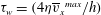 ${\it\tau}_{w}=(4{\it\eta}{\overline{v}_{x}}^{max}/h)$
and the friction Reynolds number
${\it\tau}_{w}=(4{\it\eta}{\overline{v}_{x}}^{max}/h)$
and the friction Reynolds number
 $\mathit{Re}_{\ast }=\sqrt{6\mathit{Re}}$
. Figure 9(b) shows that the Reynolds number based on the friction velocity is a little larger than
$\mathit{Re}_{\ast }=\sqrt{6\mathit{Re}}$
. Figure 9(b) shows that the Reynolds number based on the friction velocity is a little larger than
 $\sqrt{6\mathit{Re}}$
in the laminar regime, but it increases when there is a transition due to the increased wall shear stress.
$\sqrt{6\mathit{Re}}$
in the laminar regime, but it increases when there is a transition due to the increased wall shear stress.

Figure 9. The local Reynolds number
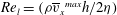 $\mathit{Re}_{l}=({\it\rho}{\overline{v}_{x}}^{max}h/2{\it\eta})$
(a) and the friction Reynolds number
$\mathit{Re}_{l}=({\it\rho}{\overline{v}_{x}}^{max}h/2{\it\eta})$
(a) and the friction Reynolds number
 $\mathit{Re}_{\ast }=({\it\rho}v_{\ast }h/{\it\eta})$
(b) as a function of the Reynolds number based on the flow rate and channel width
$\mathit{Re}_{\ast }=({\it\rho}v_{\ast }h/{\it\eta})$
(b) as a function of the Reynolds number based on the flow rate and channel width
 $\mathit{Re}=({\it\rho}Q/{\it\eta}W)$
in the zones A (○), B (▵) and C (▿) when the soft wall is made of shear modulus 18 kPa (solid lines) and 26 kPa (dashed lines). The dotted lines show the values for a two-dimensional laminar flow.
$\mathit{Re}=({\it\rho}Q/{\it\eta}W)$
in the zones A (○), B (▵) and C (▿) when the soft wall is made of shear modulus 18 kPa (solid lines) and 26 kPa (dashed lines). The dotted lines show the values for a two-dimensional laminar flow.

Figure 10. The mean velocity profiles in the zones A (○), B (▵) and C (▿) in figure 5 for a microchannel with soft wall made with shear modulus 18 kPa and Reynolds number 277 (a), shear modulus 18 kPa and Reynolds number 416 (b), shear modulus 26 kPa and Reynolds number 416 (c), and (d) the mean square of the difference in the mean velocities from experiments and ANSYS FLUENT simulations, (3.3), as a function of the Reynolds number for a microchannel with soft wall made of shear modulus 18 kPa (solid lines) and 26 kPa (dashed lines) in zones A (○), B (▵) and C (▿). In (a–c), the lines show the results obtained using the ANSYS FLUENT simulations.
The mean velocity profiles in the three different zones A, B and C (figure 5) are shown as a function of the cross-stream distance in figure 10. Also shown by the filled symbols are the results of the ANSYS FLUENT simulations for the laminar flow at the same Reynolds number. It is clearly observed that the experimental velocity profiles are flatter at the centre and steeper near the walls in comparison to the simulation results. The difference is relatively small but discernible at a Reynolds number of 277 when the soft wall is made with shear modulus 18 kPa, but the difference is much larger at a Reynolds number of 416. The mean velocity profiles do not show much variation with downstream location when the soft wall is made with shear modulus 26 kPa (possibly because there is very little variation in the height in the three different zones, as shown in figure 8 b), indicating that the flow is nearly fully developed. There is a significant change in the velocity profiles with downstream location when the soft wall is made with shear modulus 18 kPa, due to the larger height variation shown in figure 8(a). In all cases, the experimental velocity profile is significantly different from the laminar velocity profile for the same geometry when the Reynolds number exceeds the transition Reynolds number. This is in contrast to the excellent agreement between the experimental and simulation velocity profiles when the Reynolds number is below the transition Reynolds number, as shown in figure 7. A quantitative estimate of the difference between the experimental and simulation velocity profiles can be obtained by defining the scaled mean square of the difference between the experimental and simulation velocity profiles,
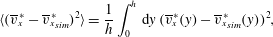 $$\begin{eqnarray}\langle ({\overline{v}_{x}}^{\!\!\ast }-{\overline{v}_{x}}_{sim}^{\!\!\ast })^{2}\rangle =\frac{1}{h}\int _{0}^{h}\,\text{d}y\,({\overline{v}_{x}}^{\!\!\ast }(y)-{\overline{v}_{x}}_{sim}^{\!\!\ast }(y))^{2},\end{eqnarray}$$
where
 ${\overline{v}_{x}}^{\!\!\ast }(y)$
is the mean velocity at the location
${\overline{v}_{x}}^{\!\!\ast }(y)$
is the mean velocity at the location
 $y$
scaled by the maximum velocity from the experiments,
$y$
scaled by the maximum velocity from the experiments,
 ${\overline{v}_{x}}_{sim}^{\!\!\ast }$
is the mean velocity predicted by the ANSYS FLUENT simulation, scaled by the maximum velocity, at the same location for a laminar flow. This measure, shown as a function of the Reynolds number in figure 10(d), is close to zero when the flow is laminar, but increases sharply after transition at a Reynolds number of 250 (in zone C) and 277 (in zones A and B) for a soft wall with shear modulus 18 kPa, and at 388 for a soft wall with shear modulus 26 kPa.
${\overline{v}_{x}}_{sim}^{\!\!\ast }$
is the mean velocity predicted by the ANSYS FLUENT simulation, scaled by the maximum velocity, at the same location for a laminar flow. This measure, shown as a function of the Reynolds number in figure 10(d), is close to zero when the flow is laminar, but increases sharply after transition at a Reynolds number of 250 (in zone C) and 277 (in zones A and B) for a soft wall with shear modulus 18 kPa, and at 388 for a soft wall with shear modulus 26 kPa.
The root mean square of the velocity fluctuations is shown as a function of the cross-stream distance in figure 11(a–c). The streamwise root mean square of the fluctuating velocity,
 $v_{x}^{\prime }$
, displays a maximum close to the wall and decreases towards the centre. This near-wall maximum in
$v_{x}^{\prime }$
, displays a maximum close to the wall and decreases towards the centre. This near-wall maximum in
 $v_{x}^{\prime }$
is clearly visible even at a Reynolds number of 277, just above the transition Reynolds number, when the soft wall is made of shear modulus 18 kPa. This near-wall maximum is a characteristic of the turbulence in a rigid channel and is attributed to the energy production due to turbulent bursts close to the wall. The
$v_{x}^{\prime }$
is clearly visible even at a Reynolds number of 277, just above the transition Reynolds number, when the soft wall is made of shear modulus 18 kPa. This near-wall maximum is a characteristic of the turbulence in a rigid channel and is attributed to the energy production due to turbulent bursts close to the wall. The
 $v_{x}^{\prime }$
profiles are clearly not symmetrical, and the value of
$v_{x}^{\prime }$
profiles are clearly not symmetrical, and the value of
 $v_{x}^{\prime }$
close to the soft wall is higher, by a factor of 2–3, in comparison to that close to the hard wall. This is very different from the flow in a rigid channel (Appendix, figure 20), where the
$v_{x}^{\prime }$
close to the soft wall is higher, by a factor of 2–3, in comparison to that close to the hard wall. This is very different from the flow in a rigid channel (Appendix, figure 20), where the
 $v_{x}^{\prime }$
profiles are symmetric about the centreline, and suggests the role of the soft wall in the production of the turbulent energy. The root mean square of the cross-stream velocity fluctuations,
$v_{x}^{\prime }$
profiles are symmetric about the centreline, and suggests the role of the soft wall in the production of the turbulent energy. The root mean square of the cross-stream velocity fluctuations,
 $v_{y}^{\prime }$
, is much smaller in magnitude than
$v_{y}^{\prime }$
, is much smaller in magnitude than
 $v_{x}^{\prime }$
, but it is also not symmetrical, and the magnitude is significantly larger near the soft wall. Figure 11(d) does indicate a shallow maximum in
$v_{x}^{\prime }$
, but it is also not symmetrical, and the magnitude is significantly larger near the soft wall. Figure 11(d) does indicate a shallow maximum in
 $v_{y}^{\prime }$
close to the wall, at a distance comparable to the distance of the maximum of
$v_{y}^{\prime }$
close to the wall, at a distance comparable to the distance of the maximum of
 $v_{x}^{\prime }$
from the wall. This is, again, very different form the flow in a rigid channel where the maximum in
$v_{x}^{\prime }$
from the wall. This is, again, very different form the flow in a rigid channel where the maximum in
 $v_{y}^{\prime }$
is further away from the wall in comparison to
$v_{y}^{\prime }$
is further away from the wall in comparison to
 $v_{x}^{\prime }$
, as shown in the Appendix in figure 20. In figure 11(a–c), we have not extrapolated the data to
$v_{x}^{\prime }$
, as shown in the Appendix in figure 20. In figure 11(a–c), we have not extrapolated the data to
 $v_{x}^{\prime }=0$
and
$v_{x}^{\prime }=0$
and
 $v_{y}^{\prime }=0$
at the soft wall, as is conventionally done in the profiles of the fluctuating velocities, since there is the possibility of velocity fluctuations at the soft wall. In order to examine the near-wall behaviour, higher-resolution images were analysed close to the wall, though we were not able to accurately resolve the region within approximately
$v_{y}^{\prime }=0$
at the soft wall, as is conventionally done in the profiles of the fluctuating velocities, since there is the possibility of velocity fluctuations at the soft wall. In order to examine the near-wall behaviour, higher-resolution images were analysed close to the wall, though we were not able to accurately resolve the region within approximately
 $10~{\rm\mu}\text{m}$
of the wall due reflections off the wall. The results of the high-resolution measurements within approximately
$10~{\rm\mu}\text{m}$
of the wall due reflections off the wall. The results of the high-resolution measurements within approximately
 $100~{\rm\mu}\text{m}$
of the wall are shown in figure 11(d). The value of
$100~{\rm\mu}\text{m}$
of the wall are shown in figure 11(d). The value of
 $v_{x}^{\prime }$
at the wall cannot be conclusively established from the results in figure 11(d); the data could plausibly be extrapolated to
$v_{x}^{\prime }$
at the wall cannot be conclusively established from the results in figure 11(d); the data could plausibly be extrapolated to
 $v_{x}^{\prime }=0$
at the wall, but the data also support a non-zero
$v_{x}^{\prime }=0$
at the wall, but the data also support a non-zero
 $v_{x}^{\prime }$
at the wall. In the case of the wall-normal velocity
$v_{x}^{\prime }$
at the wall. In the case of the wall-normal velocity
 $v_{y}^{\prime }$
, the data do not suggest a decrease to zero at the wall. This is in contrast to the flow in a rigid channel (Appendix, figure 20), where
$v_{y}^{\prime }$
, the data do not suggest a decrease to zero at the wall. This is in contrast to the flow in a rigid channel (Appendix, figure 20), where
 $v_{x}^{\prime }$
and
$v_{x}^{\prime }$
and
 $v_{y}^{\prime }$
are zero at the wall due to the no-slip condition.
$v_{y}^{\prime }$
are zero at the wall due to the no-slip condition.
Figure 11. The root mean square of the fluctuating velocities in the flow direction
 $v_{x}^{\prime }$
(solid lines and open symbols) and in the cross-stream direction
$v_{x}^{\prime }$
(solid lines and open symbols) and in the cross-stream direction
 $v_{y}^{\prime }$
(dashed lines and filled symbols) in the zones A (○), B (▵) and C (▿) in figure 5 for a microchannel with soft wall made with shear modulus 18 kPa and Reynolds number 277 (a), shear modulus 26 kPa and Reynolds number 416 (b), shear modulus 26 kPa and Reynolds number 416 (c), and a magnified view close to the soft wall of the root mean square fluctuating velocities for the soft wall made with shear modulus 18 kPa and Reynolds number 416 (d). The vertical dotted lines show, from right to left, the locations of the top wall in zones A, B and C respectively.
$v_{y}^{\prime }$
(dashed lines and filled symbols) in the zones A (○), B (▵) and C (▿) in figure 5 for a microchannel with soft wall made with shear modulus 18 kPa and Reynolds number 277 (a), shear modulus 26 kPa and Reynolds number 416 (b), shear modulus 26 kPa and Reynolds number 416 (c), and a magnified view close to the soft wall of the root mean square fluctuating velocities for the soft wall made with shear modulus 18 kPa and Reynolds number 416 (d). The vertical dotted lines show, from right to left, the locations of the top wall in zones A, B and C respectively.
The cross-correlation
 $\langle v_{x}^{\prime }v_{y}^{\prime }\rangle$
is of significance because it is proportional to the Reynolds stress, or the rate of transport of momentum due to the velocity fluctuations. As in the case of
$\langle v_{x}^{\prime }v_{y}^{\prime }\rangle$
is of significance because it is proportional to the Reynolds stress, or the rate of transport of momentum due to the velocity fluctuations. As in the case of
 $v_{x}^{\prime }$
and
$v_{x}^{\prime }$
and
 $v_{y}^{\prime }$
, the profile of
$v_{y}^{\prime }$
, the profile of
 $\langle v_{x}^{\prime }v_{y}^{\prime }\rangle$
is not symmetrical, and the zero is not at the centre of the channel, as shown in figure 12. Near the top rigid wall, the qualitative features of
$\langle v_{x}^{\prime }v_{y}^{\prime }\rangle$
is not symmetrical, and the zero is not at the centre of the channel, as shown in figure 12. Near the top rigid wall, the qualitative features of
 $\langle v_{x}^{\prime }v_{y}^{\prime }\rangle$
are similar to those for the flow in a rigid channel shown in figure 20 in the Appendix for the flow in a rigid channel, and
$\langle v_{x}^{\prime }v_{y}^{\prime }\rangle$
are similar to those for the flow in a rigid channel shown in figure 20 in the Appendix for the flow in a rigid channel, and
 $\langle v_{x}^{\prime }v_{y}^{\prime }\rangle$
does tend to zero at the top wall. However, based on the data and error in figure 12, the graph of
$\langle v_{x}^{\prime }v_{y}^{\prime }\rangle$
does tend to zero at the top wall. However, based on the data and error in figure 12, the graph of
 $\langle v_{x}^{\prime }v_{y}^{\prime }\rangle$
cannot plausibly be extrapolated to zero at the soft wall. This is significant because it implies a non-zero Reynolds stress at the soft wall and the presence of wall motion if no-slip boundary conditions are applied at the soft wall. As we show in § 3.2, wall motion is indeed detected after transition. Figure 12 shows that
$\langle v_{x}^{\prime }v_{y}^{\prime }\rangle$
cannot plausibly be extrapolated to zero at the soft wall. This is significant because it implies a non-zero Reynolds stress at the soft wall and the presence of wall motion if no-slip boundary conditions are applied at the soft wall. As we show in § 3.2, wall motion is indeed detected after transition. Figure 12 shows that
 $\langle v_{x}^{\prime }v_{y}^{\prime }\rangle$
has a maximum at the soft wall or close to the soft wall. In the following discussion, the value of
$\langle v_{x}^{\prime }v_{y}^{\prime }\rangle$
has a maximum at the soft wall or close to the soft wall. In the following discussion, the value of
 $\langle v_{x}^{\prime }v_{y}^{\prime }\rangle$
at the soft wall is determined by a cubic spline extrapolation using the four data points closest to the soft wall.
$\langle v_{x}^{\prime }v_{y}^{\prime }\rangle$
at the soft wall is determined by a cubic spline extrapolation using the four data points closest to the soft wall.

Figure 12. The root mean square of the fluctuating velocities in the flow direction
 $\langle v_{x}^{\prime }v_{y}^{\prime }\rangle$
in the zones A (○), B (▵) and C (▿) in figure 5 for a microchannel with soft wall made with shear modulus 18 kPa and Reynolds number 277 (a), shear modulus 18 kPa and Reynolds number 416 (b), and shear modulus 26 kPa and Reynolds number 416 (c). The vertical dotted lines show, from right to left, the locations of the top wall in zones A, B and C respectively.
$\langle v_{x}^{\prime }v_{y}^{\prime }\rangle$
in the zones A (○), B (▵) and C (▿) in figure 5 for a microchannel with soft wall made with shear modulus 18 kPa and Reynolds number 277 (a), shear modulus 18 kPa and Reynolds number 416 (b), and shear modulus 26 kPa and Reynolds number 416 (c). The vertical dotted lines show, from right to left, the locations of the top wall in zones A, B and C respectively.

Figure 13. The maximum values of
 $v_{x}^{\prime }$
(a),
$v_{x}^{\prime }$
(a),
 $v_{y}^{\prime }$
(b) and
$v_{y}^{\prime }$
(b) and
 $\langle v_{x}^{\prime }v_{y}^{\prime }\rangle$
(c) across the channel, scaled by suitable powers of the maximum mean velocity
$\langle v_{x}^{\prime }v_{y}^{\prime }\rangle$
(c) across the channel, scaled by suitable powers of the maximum mean velocity
 $\bar{v}_{xm}$
, as a function of the Reynolds number for soft walls made with shear modulus 18 kPa (solid line) and 26 kPa (dashed line) in zone A (○), B (▵) and C (▿) in figure 5. For comparison, the symbol ♢ shows the results at the downstream location
$\bar{v}_{xm}$
, as a function of the Reynolds number for soft walls made with shear modulus 18 kPa (solid line) and 26 kPa (dashed line) in zone A (○), B (▵) and C (▿) in figure 5. For comparison, the symbol ♢ shows the results at the downstream location
 $x=2.9~\text{cm}$
when the bottom wall is hard (shear modulus 0.55 MPa). The * symbol, referenced to the top
$x=2.9~\text{cm}$
when the bottom wall is hard (shear modulus 0.55 MPa). The * symbol, referenced to the top
 $x$
axis, shows the fluctuation intensities scaled by suitable powers of the maximum velocity from DNS (Moser, Kim & Mansour Reference Moser, Kim and Mansour1999; del Alamo et al.
Reference del Alamo, Jimenez, Zandonade and Moser2003; Hoya & Jimenez Reference Hoya and Jimenez2006) at much higher Reynolds number.
$x$
axis, shows the fluctuation intensities scaled by suitable powers of the maximum velocity from DNS (Moser, Kim & Mansour Reference Moser, Kim and Mansour1999; del Alamo et al.
Reference del Alamo, Jimenez, Zandonade and Moser2003; Hoya & Jimenez Reference Hoya and Jimenez2006) at much higher Reynolds number.
In figure 13, the maximum values of
 $v_{x}^{\prime }$
,
$v_{x}^{\prime }$
,
 $v_{y}^{\prime }$
and
$v_{y}^{\prime }$
and
 $|\langle v_{x}^{\prime }v_{y}^{\prime }\rangle |$
across the channel, scaled by suitable powers of the maximum of
$|\langle v_{x}^{\prime }v_{y}^{\prime }\rangle |$
across the channel, scaled by suitable powers of the maximum of
 $\bar{v}_{xm}$
, are shown as a function of the Reynolds number. The scaled velocities
$\bar{v}_{xm}$
, are shown as a function of the Reynolds number. The scaled velocities
 $(v_{x}^{\prime }/\bar{v}_{xm})$
and
$(v_{x}^{\prime }/\bar{v}_{xm})$
and
 $(v_{y}^{\prime }/\bar{v}_{xm})$
increase threefold from approximately 8 % to approximately 25 % and from approximately 2 % to approximately 6 % respectively at transition. The maximum of the ratio
$(v_{y}^{\prime }/\bar{v}_{xm})$
increase threefold from approximately 8 % to approximately 25 % and from approximately 2 % to approximately 6 % respectively at transition. The maximum of the ratio
 $(|\langle v_{x}^{\prime }v_{y}^{\prime }\rangle |/\bar{v}_{xm}^{2})$
also shows a threefold increase at transition. It is evident that the levels of the fluctuation intensities, scaled by the maximum velocity, vary little with Reynolds number before and after transition, but there is a near discontinuous change in the levels of the fluctuation intensities when there is a transition. Also shown in figure 13, referenced to the top
$(|\langle v_{x}^{\prime }v_{y}^{\prime }\rangle |/\bar{v}_{xm}^{2})$
also shows a threefold increase at transition. It is evident that the levels of the fluctuation intensities, scaled by the maximum velocity, vary little with Reynolds number before and after transition, but there is a near discontinuous change in the levels of the fluctuation intensities when there is a transition. Also shown in figure 13, referenced to the top
 $x$
axis, are the maximum fluctuation intensities scaled by suitable powers of the maximum velocity for a rigid channel at much higher Reynolds numbers. The scaled maximum fluctuation intensity in a soft-walled microchannel at a Reynolds number in the range 250–400 is comparable to that in a rigid-walled channel at a Reynolds number in the range 5000–20 000. The root mean square velocities scaled by the friction velocity at the soft wall have also been analysed, though the data are not shown here for conciseness. The ratio
$x$
axis, are the maximum fluctuation intensities scaled by suitable powers of the maximum velocity for a rigid channel at much higher Reynolds numbers. The scaled maximum fluctuation intensity in a soft-walled microchannel at a Reynolds number in the range 250–400 is comparable to that in a rigid-walled channel at a Reynolds number in the range 5000–20 000. The root mean square velocities scaled by the friction velocity at the soft wall have also been analysed, though the data are not shown here for conciseness. The ratio
 $v_{x}^{\prime }/v_{\ast }$
for the flow after transition in a soft-walled microchannel is approximately 20–30 % smaller, while
$v_{x}^{\prime }/v_{\ast }$
for the flow after transition in a soft-walled microchannel is approximately 20–30 % smaller, while
 $v_{y}^{\prime }/v_{\ast }$
is approximately one-half of that in a rigid-walled microchannel for Reynolds number in the range 5000–20 000. Similarly, the ratio
$v_{y}^{\prime }/v_{\ast }$
is approximately one-half of that in a rigid-walled microchannel for Reynolds number in the range 5000–20 000. Similarly, the ratio
 $\langle v_{x}^{\prime }v_{y}^{\prime }\rangle /v_{\ast }^{2}$
for the flow after transition in a soft-walled microchannel for Reynolds number in the range 250–400 is approximately one-half of that in a rigid-walled microchannel for Reynolds number in the range 5000–20 000. Thus, the fluctuation intensities in a soft-walled channel at a Reynolds number in the range 250–400 are comparable to those for a turbulent flow in a rigid channel at a Reynolds number one to two orders of magnitude higher.
$\langle v_{x}^{\prime }v_{y}^{\prime }\rangle /v_{\ast }^{2}$
for the flow after transition in a soft-walled microchannel for Reynolds number in the range 250–400 is approximately one-half of that in a rigid-walled microchannel for Reynolds number in the range 5000–20 000. Thus, the fluctuation intensities in a soft-walled channel at a Reynolds number in the range 250–400 are comparable to those for a turbulent flow in a rigid channel at a Reynolds number one to two orders of magnitude higher.
The total shear stress,
 ${\it\tau}_{xy}$
, is defined as
${\it\tau}_{xy}$
, is defined as
 $$\begin{eqnarray}{\it\tau}_{xy}={\it\eta}\frac{\partial \overline{v}_{x}}{\partial y}-{\it\rho}\langle v_{x}^{\prime }v_{y}^{\prime }\rangle ,\end{eqnarray}$$
where the velocity gradient is determined from the slope of the mean velocity profile using a cubic spline fit for the mean velocity. The total stress and the viscous stress
 ${\it\eta}(\text{d}\overline{v}_{x}/\text{d}y)$
are shown as a function of the
${\it\eta}(\text{d}\overline{v}_{x}/\text{d}y)$
are shown as a function of the
 $y$
coordinate in figure 14. The error bars are not shown in this figure for clarity. The error bars for the viscous stress are small, because the mean velocity is determined with good accuracy, as shown in figure 10. The error bars in the Reynolds stress are higher, by a factor of 1000 (density of water in SI units), in comparison to the error bars in the correlation
$y$
coordinate in figure 14. The error bars are not shown in this figure for clarity. The error bars for the viscous stress are small, because the mean velocity is determined with good accuracy, as shown in figure 10. The error bars in the Reynolds stress are higher, by a factor of 1000 (density of water in SI units), in comparison to the error bars in the correlation
 $\langle v_{x}^{\prime }v_{y}^{\prime }\rangle$
in figure 12. The Reynolds stress decreases to zero at the top rigid wall, as expected from the no-slip boundary conditions at a rigid wall. However, the Reynolds stress does not decrease to zero at the bottom soft wall, and it constitutes approximately 30 % of the total stress at the soft wall. This implies that the force exerted by the fluid on the wall contains a substantial component due to the fluid velocity fluctuations, and it is not entirely due to the viscous friction at the wall. An important feature to note is the curvature of the stress profiles. For a fully developed unidirectional flow in a channel with a constant pressure gradient, the total stress is a linear function of height. In the present experiments, the flow is not fully developed, since there is a variation in the channel height in the streamwise direction. However, the slope of the wall is numerically small, typically approximately 2 %, in the downstream sections where the velocities are measured. Therefore, the total stress is expected to be close to a linear function of the height. Figure 14 indicates that the slope of the viscous stress is certainly not a constant. However, the slope of the total stress profile is nearly a constant. In order to obtain a nearly constant slope, it is necessary to incorporate the Reynolds stress which is non-zero at the soft wall. This serves as a consistency check for the Reynolds stress which was measured independently from the velocity fluctuations; if the Reynolds stress is calculated from the pressure gradient, the values are close to those evaluated from the velocity fluctuations. The slope of the stress, which is the pressure gradient, does vary significantly with downstream position when the soft wall is made of shear modulus 18 kPa. This is due to the relatively large variation in the height of the microchannel with downstream position; this variation in the pressure gradient was observed even for a laminar flow before transition in Verma & Kumaran (Reference Verma and Kumaran2013). However, when the soft wall is made of shear modulus 26 kPa, there is a relatively small variation of approximately 20 % in the height of the microchannel and a corresponding small variation in the pressure gradient.
$\langle v_{x}^{\prime }v_{y}^{\prime }\rangle$
in figure 12. The Reynolds stress decreases to zero at the top rigid wall, as expected from the no-slip boundary conditions at a rigid wall. However, the Reynolds stress does not decrease to zero at the bottom soft wall, and it constitutes approximately 30 % of the total stress at the soft wall. This implies that the force exerted by the fluid on the wall contains a substantial component due to the fluid velocity fluctuations, and it is not entirely due to the viscous friction at the wall. An important feature to note is the curvature of the stress profiles. For a fully developed unidirectional flow in a channel with a constant pressure gradient, the total stress is a linear function of height. In the present experiments, the flow is not fully developed, since there is a variation in the channel height in the streamwise direction. However, the slope of the wall is numerically small, typically approximately 2 %, in the downstream sections where the velocities are measured. Therefore, the total stress is expected to be close to a linear function of the height. Figure 14 indicates that the slope of the viscous stress is certainly not a constant. However, the slope of the total stress profile is nearly a constant. In order to obtain a nearly constant slope, it is necessary to incorporate the Reynolds stress which is non-zero at the soft wall. This serves as a consistency check for the Reynolds stress which was measured independently from the velocity fluctuations; if the Reynolds stress is calculated from the pressure gradient, the values are close to those evaluated from the velocity fluctuations. The slope of the stress, which is the pressure gradient, does vary significantly with downstream position when the soft wall is made of shear modulus 18 kPa. This is due to the relatively large variation in the height of the microchannel with downstream position; this variation in the pressure gradient was observed even for a laminar flow before transition in Verma & Kumaran (Reference Verma and Kumaran2013). However, when the soft wall is made of shear modulus 26 kPa, there is a relatively small variation of approximately 20 % in the height of the microchannel and a corresponding small variation in the pressure gradient.

Figure 14. The shear stress
 ${\it\tau}_{xy}$
(solid line) and the viscous component of the shear stress
${\it\tau}_{xy}$
(solid line) and the viscous component of the shear stress
 $({\it\eta}\text{d}\overline{v}_{x}/\text{d}y)$
(dashed line) as a function of the cross-stream distance
$({\it\eta}\text{d}\overline{v}_{x}/\text{d}y)$
(dashed line) as a function of the cross-stream distance
 $y$
for a microchannel with soft wall made with shear modulus 18 kPa and Reynolds number 277 (a), shear modulus 18 kPa and Reynolds number 416 (b), and shear modulus 26 kPa and Reynolds number 416 (c) in zone A (○), B (▵) and C (▿).
$y$
for a microchannel with soft wall made with shear modulus 18 kPa and Reynolds number 277 (a), shear modulus 18 kPa and Reynolds number 416 (b), and shear modulus 26 kPa and Reynolds number 416 (c) in zone A (○), B (▵) and C (▿).
The rate of fluctuating energy production per unit mass,
 $-\langle v_{x}^{\prime }v_{y}^{\prime }\rangle (\text{d}\overline{v}_{x}/\text{d}y)$
, calculated from the Reynolds stress and the mean velocity gradient, is shown in figure 15. In contrast to the near-wall maximum expected for the flow near a rigid wall, it is observed that the fluctuating energy production rate is a maximum at the soft wall. This is due to the non-zero Reynolds stress and the maximum in the velocity gradient at the wall. The fluctuating energy production rate does decrease to zero at the hard upper wall and there is a maximum close to the upper wall. However, the maximum fluctuating energy production rate near the top wall is smaller, by a factor of 4, in comparison to that at the soft wall. The maximum of the fluctuating energy production rate also increases rapidly with a decrease in the channel height, both due to a significant increase in the fluid strain rate at the wall and the Reynolds stress. The rate of energy production at the wall increases sharply with an increase in the Reynolds number after transition in the downstream location C where the microchannel height is a minimum, as shown in figure 15(d), though the increase is not as large at the upstream locations A and B; this is because the strain rate at the wall is smaller at the upstream locations due to the channel expansion. The shape of the fluctuating energy production curve intriguingly suggests that the mechanism that generates velocity fluctuations is not the near-wall turbulence bursting responsible for turbulence production in the flow past a hard surface. Further work is required to establish the mechanism of near-wall fluctuating energy production near the soft wall, though the mechanism is certainly qualitatively different from that in a rigid channel.
$-\langle v_{x}^{\prime }v_{y}^{\prime }\rangle (\text{d}\overline{v}_{x}/\text{d}y)$
, calculated from the Reynolds stress and the mean velocity gradient, is shown in figure 15. In contrast to the near-wall maximum expected for the flow near a rigid wall, it is observed that the fluctuating energy production rate is a maximum at the soft wall. This is due to the non-zero Reynolds stress and the maximum in the velocity gradient at the wall. The fluctuating energy production rate does decrease to zero at the hard upper wall and there is a maximum close to the upper wall. However, the maximum fluctuating energy production rate near the top wall is smaller, by a factor of 4, in comparison to that at the soft wall. The maximum of the fluctuating energy production rate also increases rapidly with a decrease in the channel height, both due to a significant increase in the fluid strain rate at the wall and the Reynolds stress. The rate of energy production at the wall increases sharply with an increase in the Reynolds number after transition in the downstream location C where the microchannel height is a minimum, as shown in figure 15(d), though the increase is not as large at the upstream locations A and B; this is because the strain rate at the wall is smaller at the upstream locations due to the channel expansion. The shape of the fluctuating energy production curve intriguingly suggests that the mechanism that generates velocity fluctuations is not the near-wall turbulence bursting responsible for turbulence production in the flow past a hard surface. Further work is required to establish the mechanism of near-wall fluctuating energy production near the soft wall, though the mechanism is certainly qualitatively different from that in a rigid channel.

Figure 15. The fluctuating energy production rate per unit mass,
 $-\langle v_{x}^{\prime }v_{y}^{\prime }\rangle (\text{d}\overline{v}_{x}/\text{d}y)$
, as a function of the cross-stream distance
$-\langle v_{x}^{\prime }v_{y}^{\prime }\rangle (\text{d}\overline{v}_{x}/\text{d}y)$
, as a function of the cross-stream distance
 $y$
for a microchannel with soft wall made with shear modulus 18 kPa and Reynolds number 277 (a), shear modulus 18 kPa and Reynolds number 416 (b), and shear modulus 26 kPa and Reynolds number 416 (c) in zone A (○), B (▵) and C (▿), and (d) the maximum rate of fluctuating energy production per unit mass at the wall as a function of the Reynolds number for a microchannel with soft wall made of shear modulus 18 kPa (solid line) and 26 kPa (dashed line) in zone A (○), B (▵) and C (▿).
$y$
for a microchannel with soft wall made with shear modulus 18 kPa and Reynolds number 277 (a), shear modulus 18 kPa and Reynolds number 416 (b), and shear modulus 26 kPa and Reynolds number 416 (c) in zone A (○), B (▵) and C (▿), and (d) the maximum rate of fluctuating energy production per unit mass at the wall as a function of the Reynolds number for a microchannel with soft wall made of shear modulus 18 kPa (solid line) and 26 kPa (dashed line) in zone A (○), B (▵) and C (▿).

Figure 16. The reduced velocity
 $(\overline{v}_{x}/v_{\ast })$
as a function of the reduced distance
$(\overline{v}_{x}/v_{\ast })$
as a function of the reduced distance
 $(yv_{\ast }/{\it\nu})$
in the downstream zone C (figure 5) for a microchannel when the soft wall is made of shear modulus 18 kPa (a) and 26 kPa (b), and the Reynolds number is 110 (○), 222 (▵), 277 (▿), 332 (◃), 388 (▹) and 416 (♢), and for a rigid channel of height 1.52 mm at a Reynolds number of 3500 (●). Also shown are the curves for
$(yv_{\ast }/{\it\nu})$
in the downstream zone C (figure 5) for a microchannel when the soft wall is made of shear modulus 18 kPa (a) and 26 kPa (b), and the Reynolds number is 110 (○), 222 (▵), 277 (▿), 332 (◃), 388 (▹) and 416 (♢), and for a rigid channel of height 1.52 mm at a Reynolds number of 3500 (●). Also shown are the curves for
 $(\overline{v}_{x}/v_{\ast })=(yv_{\ast }/{\it\nu})$
(dotted line),
$(\overline{v}_{x}/v_{\ast })=(yv_{\ast }/{\it\nu})$
(dotted line),
 $(\overline{v}_{x}/v_{\ast })=2.5\log (yv_{\ast }/{\it\nu})+5$
(dashed line),
$(\overline{v}_{x}/v_{\ast })=2.5\log (yv_{\ast }/{\it\nu})+5$
(dashed line),
 $(\overline{v}_{x}/v_{\ast })=3\log (yv_{\ast }/{\it\nu})-2.3$
(solid line in (a)) and
$(\overline{v}_{x}/v_{\ast })=3\log (yv_{\ast }/{\it\nu})-2.3$
(solid line in (a)) and
 $(\overline{v}_{x}/v_{\ast })=2.8\log (yv_{\ast }/{\it\nu})-2.3$
(solid line in (b)). The data collapse can be compared with the dimensional velocity profiles shown in figure 10.
$(\overline{v}_{x}/v_{\ast })=2.8\log (yv_{\ast }/{\it\nu})-2.3$
(solid line in (b)). The data collapse can be compared with the dimensional velocity profiles shown in figure 10.
The viscous sublayer and the logarithmic layer close to the wall are universal features of turbulent flows near rigid surfaces. The viscous sublayer with a linear profile extends up to
 $(yv_{\ast }/{\it\nu})\sim 10$
and the velocity is given by
$(yv_{\ast }/{\it\nu})\sim 10$
and the velocity is given by
 $(\overline{v}_{x}/v_{\ast })=(yv_{\ast }/{\it\nu})$
, and the logarithmic layer extends from
$(\overline{v}_{x}/v_{\ast })=(yv_{\ast }/{\it\nu})$
, and the logarithmic layer extends from
 $30<(yv_{\ast }/{\it\nu})<200$
where the velocity profile satisfies the von Karman law
$30<(yv_{\ast }/{\it\nu})<200$
where the velocity profile satisfies the von Karman law
 $(\overline{v}_{x}/v_{\ast })=A\log (yv_{\ast }/{\it\nu})+B$
, where
$(\overline{v}_{x}/v_{\ast })=A\log (yv_{\ast }/{\it\nu})+B$
, where
 $A$
and
$A$
and
 $B$
are the von Karman constants. Here,
$B$
are the von Karman constants. Here,
 $v_{\ast }=\sqrt{{\it\tau}_{w}/{\it\rho}}$
is the friction velocity, and
$v_{\ast }=\sqrt{{\it\tau}_{w}/{\it\rho}}$
is the friction velocity, and
 ${\it\tau}_{w}$
is the wall shear stress at the soft wall shown in figure 14. Here, an attempt has been made to examine the velocity profile close to the wall, to check whether there is a discernible viscous sublayer and logarithmic layer in the flow past a soft surface. The results for the variation of the reduced velocity
${\it\tau}_{w}$
is the wall shear stress at the soft wall shown in figure 14. Here, an attempt has been made to examine the velocity profile close to the wall, to check whether there is a discernible viscous sublayer and logarithmic layer in the flow past a soft surface. The results for the variation of the reduced velocity
 $(\overline{v}_{x}/v_{\ast })$
with the reduced distance
$(\overline{v}_{x}/v_{\ast })$
with the reduced distance
 $(yv_{\ast }/{\it\nu})$
are shown in figure 16. Also shown, for comparison, is the velocity profile in a rigid channel at a Reynolds number of 3500 from the experiments discussed in the Appendix. The velocity profile in the rigid channel shows evidence of a viscous sublayer with the scaling
$(yv_{\ast }/{\it\nu})$
are shown in figure 16. Also shown, for comparison, is the velocity profile in a rigid channel at a Reynolds number of 3500 from the experiments discussed in the Appendix. The velocity profile in the rigid channel shows evidence of a viscous sublayer with the scaling
 $(\overline{v}_{x}/v_{\ast })=(yv_{\ast }/{\it\nu})$
for
$(\overline{v}_{x}/v_{\ast })=(yv_{\ast }/{\it\nu})$
for
 $(yv_{\ast }/{\it\nu})<5$
. After this, there is a transition to a profile that seems to agree well with the logarithmic law
$(yv_{\ast }/{\it\nu})<5$
. After this, there is a transition to a profile that seems to agree well with the logarithmic law
 $(\overline{v}_{x}/v_{\ast })=2.5\log (yv_{\ast }/{\it\nu})+5.0$
, even though the Reynolds number of 3500 for the rigid channel is a little low. In the case of the flow through the microchannel, there is a data collapse when we plot
$(\overline{v}_{x}/v_{\ast })=2.5\log (yv_{\ast }/{\it\nu})+5.0$
, even though the Reynolds number of 3500 for the rigid channel is a little low. In the case of the flow through the microchannel, there is a data collapse when we plot
 $(\overline{v}_{x}/v_{\ast })$
as a function of
$(\overline{v}_{x}/v_{\ast })$
as a function of
 $(yv_{\ast }/{\it\nu})$
only after transition, that is, for Reynolds numbers higher than 277 when the soft wall is made of shear modulus 18 kPa and higher than 332 when the soft wall is made of shear modulus 26 kPa. There is no evidence of the linear profile
$(yv_{\ast }/{\it\nu})$
only after transition, that is, for Reynolds numbers higher than 277 when the soft wall is made of shear modulus 18 kPa and higher than 332 when the soft wall is made of shear modulus 26 kPa. There is no evidence of the linear profile
 $(\overline{v}_{x}/v_{\ast })=(yv_{\ast }/{\it\nu})$
expected for a viscous sublayer even for
$(\overline{v}_{x}/v_{\ast })=(yv_{\ast }/{\it\nu})$
expected for a viscous sublayer even for
 $(yv_{\ast }/{\it\nu})$
as low as 2, though a viscous sublayer for smaller values of
$(yv_{\ast }/{\it\nu})$
as low as 2, though a viscous sublayer for smaller values of
 $(yv_{\ast }/{\it\nu})$
cannot be ruled out based on our data which extend only up to
$(yv_{\ast }/{\it\nu})$
cannot be ruled out based on our data which extend only up to
 $(yv_{\ast }/{\it\nu})\sim 2$
. The logarithmic layer seems to extend from
$(yv_{\ast }/{\it\nu})\sim 2$
. The logarithmic layer seems to extend from
 $(yv_{\ast }/{\it\nu})=4$
to approximately
$(yv_{\ast }/{\it\nu})=4$
to approximately
 $(yv_{\ast }/{\it\nu})=30$
. This is in contrast to the logarithmic layer in a pipe flow which extends from
$(yv_{\ast }/{\it\nu})=30$
. This is in contrast to the logarithmic layer in a pipe flow which extends from
 $(yv_{\ast }/{\it\nu})=30$
to approximately
$(yv_{\ast }/{\it\nu})=30$
to approximately
 $(yv_{\ast }/{\it\nu})=200$
. In the logarithmic layer, the velocity profile seems to follow the equation
$(yv_{\ast }/{\it\nu})=200$
. In the logarithmic layer, the velocity profile seems to follow the equation
 $(\overline{v}_{x}/v_{\ast })=A\log (yv_{\ast }/{\it\nu})+B$
, where best fits are obtained when
$(\overline{v}_{x}/v_{\ast })=A\log (yv_{\ast }/{\it\nu})+B$
, where best fits are obtained when
 $A$
assumes slightly different values of 3.0 and 2.8 for soft walls made with shear modulus 18 kPa and 26 kPa, and
$A$
assumes slightly different values of 3.0 and 2.8 for soft walls made with shear modulus 18 kPa and 26 kPa, and
 $B$
has a value of approximately
$B$
has a value of approximately
 $-2.3$
in both cases.
$-2.3$
in both cases.
In contrast to the universal logarithmic law for the mean velocity when scaled by the friction velocity, it has been known for some time now that the fluctuating velocity, scaled by the friction velocity, does not exhibit universal ‘wall scaling’ when expressed as a function of
 $(yv_{\ast }/{\it\nu})$
. This has been interpreted as an indication that the large-scale fluctuations in the outer flow far from the wall affect the turbulent bursting near the wall (Rao, Narasimha & Badri Narayanan Reference Rao, Narasimha and Badri Narayanan1971; Marusic et al.
Reference Marusic, McKeon, Monkewitz, Nagib, Smits and Sreenivasan2010) which generates the near-wall velocity fluctuations. It is of interest to examine whether this lack of ‘wall scaling’ is also observed for the flow at small dimensions and low Reynolds number. The root mean square of the streamwise fluctuating velocity, scaled by the friction velocity, is shown as a function of the scaled distance
$(yv_{\ast }/{\it\nu})$
. This has been interpreted as an indication that the large-scale fluctuations in the outer flow far from the wall affect the turbulent bursting near the wall (Rao, Narasimha & Badri Narayanan Reference Rao, Narasimha and Badri Narayanan1971; Marusic et al.
Reference Marusic, McKeon, Monkewitz, Nagib, Smits and Sreenivasan2010) which generates the near-wall velocity fluctuations. It is of interest to examine whether this lack of ‘wall scaling’ is also observed for the flow at small dimensions and low Reynolds number. The root mean square of the streamwise fluctuating velocity, scaled by the friction velocity, is shown as a function of the scaled distance
 $(yv_{\ast }/{\it\nu})$
in figure 17. The data for the scaled fluctuating velocity
$(yv_{\ast }/{\it\nu})$
in figure 17. The data for the scaled fluctuating velocity
 $v_{x}^{\prime }$
do not collapse onto a single curve, in contrast to those for the mean velocity in figure 16. This is similar to turbulence in a channel with rigid walls, where also it is observed that the streamwise root mean square velocity does not exhibit scaling when expressed in terms of inner variables. However, there is an important difference from rigid-wall-bounded turbulence. The location of the maximum in figure 17, approximately
$v_{x}^{\prime }$
do not collapse onto a single curve, in contrast to those for the mean velocity in figure 16. This is similar to turbulence in a channel with rigid walls, where also it is observed that the streamwise root mean square velocity does not exhibit scaling when expressed in terms of inner variables. However, there is an important difference from rigid-wall-bounded turbulence. The location of the maximum in figure 17, approximately
 $(yv_{\ast }/{\it\nu})=8$
, is smaller than the value of approximately 15 usually reported for the flow past a rigid surface at much higher Reynolds number. In figure 17, the maximum value of
$(yv_{\ast }/{\it\nu})=8$
, is smaller than the value of approximately 15 usually reported for the flow past a rigid surface at much higher Reynolds number. In figure 17, the maximum value of
 $(v_{x}^{\prime }/v_{\ast })$
is in the range 1.8–2.3, which is not much smaller than the maximum of 2.8–3 for the flow past a rigid surface at Reynolds numbers approximately two to three orders of magnitude higher. It should be noted that
$(v_{x}^{\prime }/v_{\ast })$
is in the range 1.8–2.3, which is not much smaller than the maximum of 2.8–3 for the flow past a rigid surface at Reynolds numbers approximately two to three orders of magnitude higher. It should be noted that
 $(v_{x}^{\prime }/v_{\ast })$
is large only near the soft wall; it is smaller by a factor of at least two near the hard wall.
$(v_{x}^{\prime }/v_{\ast })$
is large only near the soft wall; it is smaller by a factor of at least two near the hard wall.

Figure 17. The root mean square of the streamwise fluctuating velocities,
 $(v_{x}^{\prime }/v_{\ast })$
, as a function of the reduced distance
$(v_{x}^{\prime }/v_{\ast })$
, as a function of the reduced distance
 $(yv_{\ast }/{\it\nu})$
in the downstream zone C (figure 5) for a microchannel when the soft wall is made of shear modulus 18 kPa (a) and 26 kPa (b), and the Reynolds number is 110 (○), 222 (▵), 277 (▿), 332 (◃), 388 (▹) and 416 (♢).
$(yv_{\ast }/{\it\nu})$
in the downstream zone C (figure 5) for a microchannel when the soft wall is made of shear modulus 18 kPa (a) and 26 kPa (b), and the Reynolds number is 110 (○), 222 (▵), 277 (▿), 332 (◃), 388 (▹) and 416 (♢).
3.2. Wall displacement
The average displacement of the soft wall in the streamwise direction,
 $\bar{u}_{x}$
, at the fluid–wall interface, as measured by the motion of the ink spot discussed in § 2.3, is shown in figure 18(a). There is a displacement of up to
$\bar{u}_{x}$
, at the fluid–wall interface, as measured by the motion of the ink spot discussed in § 2.3, is shown in figure 18(a). There is a displacement of up to
 $10~{\rm\mu}\text{m}$
in the soft wall with shear modulus 18 kPa, and approximately
$10~{\rm\mu}\text{m}$
in the soft wall with shear modulus 18 kPa, and approximately
 $6~{\rm\mu}\text{m}$
for the soft wall with shear modulus 26 kPa. Also shown in figure 18(a), by the filled symbols, is the expected displacement from the fluid shear stress at the wall, shown in figure 14, in zone B (figure 5) where the dye spot is located. The expected displacement is calculated as the strain (ratio of the wall shear stress and the shear modulus) times the thickness (2 mm) of the bottom wall. The observed mean displacement is in good quantitative agreement with that expected from the shear stress exerted on the soft wall. It should be mentioned that there is a much larger displacement of the order of
$6~{\rm\mu}\text{m}$
for the soft wall with shear modulus 26 kPa. Also shown in figure 18(a), by the filled symbols, is the expected displacement from the fluid shear stress at the wall, shown in figure 14, in zone B (figure 5) where the dye spot is located. The expected displacement is calculated as the strain (ratio of the wall shear stress and the shear modulus) times the thickness (2 mm) of the bottom wall. The observed mean displacement is in good quantitative agreement with that expected from the shear stress exerted on the soft wall. It should be mentioned that there is a much larger displacement of the order of
 $100~{\rm\mu}\text{m}$
in the wall-normal direction as the Reynolds number increases, as is evident from figure 8. Despite this, the displacement tangential to the wall is accurately measured and correlates well with the shear stress exerted on the wall. The root mean squares of the displacement in the streamwise and spanwise directions,
$100~{\rm\mu}\text{m}$
in the wall-normal direction as the Reynolds number increases, as is evident from figure 8. Despite this, the displacement tangential to the wall is accurately measured and correlates well with the shear stress exerted on the wall. The root mean squares of the displacement in the streamwise and spanwise directions,
 $u_{x}^{\prime }$
and
$u_{x}^{\prime }$
and
 $u_{z}^{\prime }$
, calculated from the displacement time series, are shown in figure 18(b). The root mean square displacements
$u_{z}^{\prime }$
, calculated from the displacement time series, are shown in figure 18(b). The root mean square displacements
 $u_{x}^{\prime }$
and
$u_{x}^{\prime }$
and
 $u_{y}^{\prime }$
are non-zero even at zero Reynolds number, due to lack of experimental resolution of distances below approximately
$u_{y}^{\prime }$
are non-zero even at zero Reynolds number, due to lack of experimental resolution of distances below approximately
 $1~{\rm\mu}\text{m}$
. However, a sharp increase in the root mean square displacements in both the streamwise and spanwise directions occurs at the flow transition Reynolds number. The root mean squares of the wall displacement fluctuations are relatively small, of the order of
$1~{\rm\mu}\text{m}$
. However, a sharp increase in the root mean square displacements in both the streamwise and spanwise directions occurs at the flow transition Reynolds number. The root mean squares of the wall displacement fluctuations are relatively small, of the order of
 $1{-}2~{\rm\mu}\text{m}$
, but these are clearly discernible in figure 18(b), as well as the time traces of the fluctuations in the position of the dye spot discussed next. This confirms the onset of wall motion coupled with the transition in the fluid.
$1{-}2~{\rm\mu}\text{m}$
, but these are clearly discernible in figure 18(b), as well as the time traces of the fluctuations in the position of the dye spot discussed next. This confirms the onset of wall motion coupled with the transition in the fluid.

Figure 18. The steady displacement in the streamwise direction (a) and the root mean square of the fluctuations in the displacement in the streamwise (solid line) and spanwise (dashed line) directions (b) for the flow through a microchannel with soft wall made of shear modulus 18 kPa (○) and 26 kPa (▵). The filled symbols in (a) show the mean displacement calculated from the wall shear stress in the fluid and the shear modulus and thickness of the soft wall.
A more detailed picture of the wall fluctuations is obtained from the time variation of the displacement, measured as discussed in § 2.3. The time series of the streamwise displacement at different Reynolds numbers are shown in figure 19. High-frequency fluctuations are present even in the laminar regime, due to background noise and the noise in the CCD sensors of the camera. However, after transition (for Reynolds number greater than 250 for a soft wall with shear modulus 18 kPa in figure 19(a) and Reynolds number greater than 332 for a soft wall with shear modulus 26 kPa in figure 19(b)), variations at much lower frequency are visible in figure 19. The amplitudes of the fluctuations are relatively small, of the order of
 $1{-}2~{\rm\mu}\text{m}$
, but these fluctuations are clearly discernible in the time traces in figure 19(a,b). Based on the linear stability analysis (Verma & Kumaran Reference Verma and Kumaran2013), the frequency of the most unstable modes is expected to be
$1{-}2~{\rm\mu}\text{m}$
, but these fluctuations are clearly discernible in the time traces in figure 19(a,b). Based on the linear stability analysis (Verma & Kumaran Reference Verma and Kumaran2013), the frequency of the most unstable modes is expected to be
 $10^{3}{-}10^{4}~\text{Hz}$
. Such high frequencies cannot be measured with the imaging procedure used here, because the Nyquist frequency is 500 Hz for our imaging system with a framing rate of 1000 f.p.s.; considering an oversampling factor of 10, a framing rate of at least
$10^{3}{-}10^{4}~\text{Hz}$
. Such high frequencies cannot be measured with the imaging procedure used here, because the Nyquist frequency is 500 Hz for our imaging system with a framing rate of 1000 f.p.s.; considering an oversampling factor of 10, a framing rate of at least
 $10^{4}{-}10^{5}~\text{Hz}$
is required for capturing the frequencies predicted by the linear analysis. However, even with the present sampling rates, the appearance of relatively low-frequency structure after transition is also evident in the frequency spectra of the displacement shown in figure 19(c,d).
$10^{4}{-}10^{5}~\text{Hz}$
is required for capturing the frequencies predicted by the linear analysis. However, even with the present sampling rates, the appearance of relatively low-frequency structure after transition is also evident in the frequency spectra of the displacement shown in figure 19(c,d).

Figure 19. Time series (a,b) and frequency spectra (c,d) of the displacement of a dye spot in the streamwise direction at different Reynolds numbers when the soft wall is made with shear modulus 18 kPa (a,c) and 26 kPa (b,d). The curves are displaced vertically with respect to each other to enhance clarity, and the dotted lines show the baseline for each curve.
The observation of a non-zero stress at the wall and wall displacement suggests that the mechanism of fluctuating energy production may be different from that in rigid-walled channels, where the production term is given by
 $-{\it\rho}\langle v_{x}^{\prime }v_{y}^{\prime }\rangle (\text{d}\bar{v}_{x}/\text{d}y)$
due to the interaction of the Reynolds stress and the mean velocity gradient. Linear stability studies (Verma & Kumaran Reference Verma and Kumaran2013) indicate that the mechanism of destabilisation of the laminar flow is the transfer of energy from the mean flow to the fluctuations due to the shear work done at the fluid–solid interface. The rate at which shear work is done,
$-{\it\rho}\langle v_{x}^{\prime }v_{y}^{\prime }\rangle (\text{d}\bar{v}_{x}/\text{d}y)$
due to the interaction of the Reynolds stress and the mean velocity gradient. Linear stability studies (Verma & Kumaran Reference Verma and Kumaran2013) indicate that the mechanism of destabilisation of the laminar flow is the transfer of energy from the mean flow to the fluctuations due to the shear work done at the fluid–solid interface. The rate at which shear work is done,
 $\mathscr{S}$
, at the interface is the product of the shear stress and the tangential velocity integrated over the surface,
$\mathscr{S}$
, at the interface is the product of the shear stress and the tangential velocity integrated over the surface,
 $$\begin{eqnarray}\mathscr{S}=\int \text{d}S\,\boldsymbol{v}\boldsymbol{\cdot }{\it\tau}\boldsymbol{\cdot }\boldsymbol{n},\end{eqnarray}$$
where
 $\text{d}S$
is the differential surface area and
$\text{d}S$
is the differential surface area and
 $\boldsymbol{n}$
is the outward unit normal to the surface. When there is a no-slip condition at the surface, the tangential velocity is zero and so the shear work is zero. When there is a steady flow, the tangential velocity at the surface is once again zero (though there is a non-zero tangential displacement), and the shear work done at the interface is once again zero. When there are fluctuations, it is convenient to separate the tangential velocity at the surface into its mean and fluctuating components,
$\boldsymbol{n}$
is the outward unit normal to the surface. When there is a no-slip condition at the surface, the tangential velocity is zero and so the shear work is zero. When there is a steady flow, the tangential velocity at the surface is once again zero (though there is a non-zero tangential displacement), and the shear work done at the interface is once again zero. When there are fluctuations, it is convenient to separate the tangential velocity at the surface into its mean and fluctuating components,
 $v_{x}=\bar{v}_{x}+v_{x}^{\prime }$
. The rates of shear work done by the fluctuations on the fluid side
$v_{x}=\bar{v}_{x}+v_{x}^{\prime }$
. The rates of shear work done by the fluctuations on the fluid side
 $\mathscr{S}_{f}$
and the solid side
$\mathscr{S}_{f}$
and the solid side
 $\mathscr{S}_{s}$
are
$\mathscr{S}_{s}$
are
 $$\begin{eqnarray}\displaystyle & \mathscr{S}_{f}^{\prime }=-\displaystyle \int \text{d}S\,({\it\tau}_{xy}v_{x}^{\prime })|_{f}, & \displaystyle\end{eqnarray}$$
 $$\begin{eqnarray}\displaystyle & \mathscr{S}_{s}^{\prime }=\displaystyle \int \text{d}S\left.\left({\it\tau}_{xy}\frac{\text{D}u_{x}^{\prime }}{\text{D}t}\right)\right|_{s}, & \displaystyle\end{eqnarray}$$
 $f$
and
$f$
and
 $s$
refer to fluid and solid respectively, and the velocity fluctuation in the solid has been set equal to the substantial derivative of the surface displacement,
$s$
refer to fluid and solid respectively, and the velocity fluctuation in the solid has been set equal to the substantial derivative of the surface displacement,
 $(\text{D}u_{x}^{\prime }/\text{D}t)$
(the time rate of change of the mean displacement is zero). There is a negative sign in the expression for the shear work on the fluid side, because the outward unit normal is directed in the
$(\text{D}u_{x}^{\prime }/\text{D}t)$
(the time rate of change of the mean displacement is zero). There is a negative sign in the expression for the shear work on the fluid side, because the outward unit normal is directed in the
 $-y$
direction. When there is stress continuity, the shear stresses at the surface are equal on the fluid and solid sides. However, the velocity fluctuations on the two sides are not equal when the surface is displaced. For a surface displacement
$-y$
direction. When there is stress continuity, the shear stresses at the surface are equal on the fluid and solid sides. However, the velocity fluctuations on the two sides are not equal when the surface is displaced. For a surface displacement
 $u_{y}^{\prime }$
, the mean velocity at the displaced surface on the fluid side is
$u_{y}^{\prime }$
, the mean velocity at the displaced surface on the fluid side is
 $(\text{d}\bar{v}_{x}/\text{d}y)u_{y}^{\prime }$
, where
$(\text{d}\bar{v}_{x}/\text{d}y)u_{y}^{\prime }$
, where
 $(\text{d}\bar{v}_{x}/\text{d}y)$
is the mean strain rate, while the mean velocity at the displaced surface on the solid side is zero, since there is no mean motion in the solid. Therefore, the no-slip condition at the displaced surface, linearised about the base surface configuration, is
$(\text{d}\bar{v}_{x}/\text{d}y)$
is the mean strain rate, while the mean velocity at the displaced surface on the solid side is zero, since there is no mean motion in the solid. Therefore, the no-slip condition at the displaced surface, linearised about the base surface configuration, is  $$\begin{eqnarray}v_{x}^{\prime }+\frac{\text{d}\bar{v}_{x}}{\text{d}y}u_{y}^{\prime }=\frac{\text{D}u_{x}^{\prime }}{\text{D}t}.\end{eqnarray}$$
Due to this additional term in the velocity condition at the interface, the rates of shear work on the fluid and solid sides do not sum to zero,
 $$\begin{eqnarray}\mathscr{S}^{\prime }=\mathscr{S}_{f}^{\prime }+\mathscr{S}_{s}^{\prime }=\displaystyle \int \text{d}S\,{\it\tau}_{xy}u_{y}^{\prime }\,\frac{\text{d}\bar{v}_{x}}{\text{d}y}.\end{eqnarray}$$
When the stress is separated into a mean and a fluctuating part,
 ${\it\tau}_{xy}=\bar{{\it\tau}}_{xy}+{\it\tau}_{xy}^{\prime }$
, the correlations between the stress fluctuations
${\it\tau}_{xy}=\bar{{\it\tau}}_{xy}+{\it\tau}_{xy}^{\prime }$
, the correlations between the stress fluctuations
 ${\it\tau}_{xy}^{\prime }$
and the displacement fluctuations
${\it\tau}_{xy}^{\prime }$
and the displacement fluctuations
 $u_{y}^{\prime }$
can be non-zero, resulting a transfer of energy from the mean flow to the fluctuations which destabilises the laminar flow (Kumaran Reference Kumaran1995). While this mechanism is well established for the flow instability, it has not yet been demonstrated for energy production after transition. Although this provides a plausible mechanism different from the usual fluctuating energy production, a lot more theoretical work is required to conclusively establish the energy production mechanism in the present case.
$u_{y}^{\prime }$
can be non-zero, resulting a transfer of energy from the mean flow to the fluctuations which destabilises the laminar flow (Kumaran Reference Kumaran1995). While this mechanism is well established for the flow instability, it has not yet been demonstrated for energy production after transition. Although this provides a plausible mechanism different from the usual fluctuating energy production, a lot more theoretical work is required to conclusively establish the energy production mechanism in the present case.
4. Conclusions
Previous experimental results (Verma & Kumaran Reference Verma and Kumaran2013) have shown that the flow is highly diffusive, and the diffusivity in the spanwise direction is five orders of magnitude larger than the molecular diffusivity in a laminar flow. The present experiments reveal that the flow is also three-dimensional, and the magnitude of the fluctuating velocities is large even in the wall-normal direction, indicating that the flow after transition can be characterised as a turbulent flow. When compared with hard-wall-bounded turbulence, the flow characteristics are similar in many ways, but are also qualitatively different in important respects.
-
(1) After transition, the mean velocity profile measured in the experiments exhibits a distinct departure from the velocity profile for the laminar flow in a deformed channel of the same dimensions and flow rate. The qualitative nature of the mean velocity profile, which is flatter at the centre and steeper at the walls when compared with the velocity profile for a laminar flow, is similar to that observed in turbulent flow in a rigid channel.
-
(2) The flow also exhibits many of the characteristics observed in rigid-wall-bounded turbulence, such as the prominent near-wall maximum in the streamwise root mean square of the fluctuating velocity and the much smaller magnitude of the cross-stream root mean square fluctuating velocity. However, there are also important differences. The most important is the asymmetry in the profiles of
 $v_{x}^{\prime }$
, where the maximum near the soft wall is at least two times higher than that near the hard wall. This points to the role of the soft surface in the generation of turbulent velocity fluctuations.
$v_{x}^{\prime }$
, where the maximum near the soft wall is at least two times higher than that near the hard wall. This points to the role of the soft surface in the generation of turbulent velocity fluctuations. -
(3) It also appears that
$v_{x}^{\prime }$
and
$v_{y}^{\prime }$
may not decrease to zero at the soft surface, in contrast to the rigid surface where the velocity fluctuations are zero due to the no-slip conditions at a rigid surface. This indicates that there is the onset of wall motion coupled with the fluid velocity fluctuations. Wall fluctuations are indeed observed after transition, as noted in points (9) and (10) below. -
(4) The experiments also indicate that the Reynolds stress is non-zero at the soft surface, and the Reynolds stress constitutes up to 30 % of the total stress at the soft surface. Once again, this is in contrast to the flow past a rigid surface, where the Reynolds stress decreases to zero due to the zero-velocity condition at the surface.
-
(5) The fluctuating energy production rate has a maximum at the wall, in contrast to the near-wall maximum in the flow past hard surfaces. This suggests that the fluctuating energy production mechanism is not the near-wall bursting of eddies for the turbulent flow in a rigid channel.
-
(6) When compared with the turbulence in a rigid channel at Reynolds number in the range 5000–21 000, the maximum of the root mean square streamwise fluctuating velocity
$v_{x}^{\prime }$
at Reynolds number 250–400 is larger, the maximum of the root mean square cross-stream fluctuating velocity
$v_{y}^{\prime }$
is comparable and the maximum of the correlation
$\langle v_{x}^{\prime }v_{y}^{\prime }\rangle$
is significantly higher when scaled by suitable powers of the maximum velocity. Even when scaled by suitable powers of the friction velocity,
$v_{x}^{\prime }$
is smaller by approximately 30 %,
$v_{y}^{\prime }$
is approximately one-half and
$\langle v_{x}^{\prime }v_{y}^{\prime }\rangle$
is approximately one-half of that in a rigid channel at Reynolds number in the range 5000–20 000. -
(7) Logarithmic variation of the mean velocity with distance from the wall, characteristic of the ‘logarithmic layer’ in the flow past rigid surfaces, is also observed here. Although the logarithmic law is found to apply close to the surface, the von Karman constants are very different from those for the flow past hard surfaces and, based on the limited data available, they seem to depend on the shear modulus of the soft wall. The logarithmic law was found to be valid approximately in the range
$5\leqslant (yv_{\ast }/{\it\nu})\leqslant 30$
; both the lower and the upper limits of this range are much smaller than those for the flow past a hard wall. It is not clear whether these constants and the range of validity would smoothly transition to those for a hard wall. A viscous sublayer with a linear velocity profile was not detected in the experiments, where it was not possible to resolve velocities within approximately
$10~{\rm\mu}\text{m}$
of the surface. It is not clear whether there is a viscous sublayer that extends to wall-normal distances of less than
$10~{\rm\mu}\text{m}$
, or whether the layer itself is disrupted by wall motion. A relevant point of reference is the thickness of the Stokes layer near a boundary oscillating with the frequency of the soft wall predicted by the stability analysis at transition. Linear stability analysis (Verma & Kumaran Reference Verma and Kumaran2013) predicts that the frequency of the most unstable modes is approximately
$(10^{-3}G/{\it\eta})\sim 2\times 10^{4}~\text{Hz}$
for shear modulus
$G$
of approximately
$2\times 10^{4}~\text{Pa}$
and viscosity of
$10^{-3}~\text{kg}~\text{m}~\text{s}^{-1}$
. The thickness of the Stokes layer,
$(2{\it\nu}/{\it\omega})^{1/2}$
, is then approximately
$300~{\rm\mu}\text{m}$
, which is larger than the thickness of the microchannel. Therefore, it is possible that there is a disruption of the near-wall linear velocity profile due to wall mobilisation. -
(8) Other more subtle characteristics, such as the lack of ‘wall scaling’ when
$(v_{x}^{\prime }/v_{\ast })$
is expressed as a function of
$(yv_{\ast }/{\it\nu})$
, are also observed in the experiments at Reynolds numbers as low as 250. -
(9) The experiments also clearly show the presence of wall deformation and wall motion in the flow. The tangential surface displacement due to the applied stress is small, of the order of a few microns, as expected from the relative magnitudes of the fluid stress and the elasticity modulus of the wall material. The maximum fluid stress is approximately 100 Pa (as shown in figure 14), while the shear modulus of the soft material is approximately
$2\times 10^{4}~\text{Pa}$
. This results in a small strain of
$5\times 10^{-3}$
, which, for a material of thickness 2 mm, results in a displacement of approximately
$10~{\rm\mu}\text{m}$
. -
(10) After transition, there is a discernible increase in the magnitude of the displacement fluctuations in the wall, of the order of
$1{-}2~{\rm\mu}\text{m}$
. This indicates the advent of wall oscillations coupled with fluid velocity fluctuations at transition. The experiments were limited in their time resolution, and were able to resolve the fluctuations only up to a few 100 Hz. We do observe the appearance of low-frequency structure in the power spectrum of the displacement fluctuations after transition. Linear stability analysis indicates that the most unstable modes have a much higher frequency, of the order of
$2\times 10^{4}~\text{Hz}$
(Verma & Kumaran Reference Verma and Kumaran2013). More sophisticated measurements are required to resolve these high-frequency fluctuations in order to gain insight into the nature of wall motion.


There is also an unresolved issue regarding the non-zero velocity fluctuations at the interface. Based on the frequency of
 $2\times 10^{4}~\text{Hz}$
predicted by the linear stability analysis and the amplitude of oscillations of approximately a micron, the velocity of the surface of the soft material is of the order of
$2\times 10^{4}~\text{Hz}$
predicted by the linear stability analysis and the amplitude of oscillations of approximately a micron, the velocity of the surface of the soft material is of the order of
 $0.02~\text{m}~\text{s}^{-1}$
. Velocities of this magnitude could be obtained by extrapolation of the fluctuating velocities to the wall (figure 11). However, direct measurements of the high-frequency fluctuations are necessary to confirm this.
$0.02~\text{m}~\text{s}^{-1}$
. Velocities of this magnitude could be obtained by extrapolation of the fluctuating velocities to the wall (figure 11). However, direct measurements of the high-frequency fluctuations are necessary to confirm this.
The experimental results presented here indicate that the flow after transition in a microchannel with a soft viscoelastic wall can certainly be characterised as turbulent. This suggests that there is fluid turbulence at a Reynolds number smaller, by approximately an order of magnitude, in comparison to that observed in the flow past rigid surfaces. The striking qualitative differences between the present flow characteristics and those at a rigid surface suggest that soft-wall-bounded turbulence involving wall mobilisation belongs to a separate class of turbulent flows, distinct from hard-wall-bounded turbulence. This augments the now established distinct transition mechanism in the flow past soft surfaces, due to a linear instability caused by a coupling between the fluid and the wall dynamics. These distinctions could have a significant impact on the flow dynamics and transport processes in flows past soft surfaces both in microfluidic devices where conduits are made of soft materials and in biological systems where fluids are transported through soft tubes.
Acknowledgements
The authors would like to thank the Department of Science and Technology, Government of India for financial support. The authors gratefully acknowledge the experimental facilities made available and the advice provided by Professors O. N. Ramesh, J. Dey, R. Govardhan, J. H. Arakeri, A. Ghosh and S. V. Kailas. The authors are grateful to Professor A. C. Mandal, Dr M. K. S. Verma, Mr J. S. Murthy, Mr P. Kumar, Mr N. Jha, Mr V. Swamybabu and Ms L. Venugopalan for instructive discussions and help with the experiments.
Appendix. Validation of turbulence measurements
For the test channels, rectangular channels of cross-section dimensions
 $1.52~\text{mm}\times 1.5~\text{cm}$
and length approximately 20 cm were fabricated using template-assisted lithography in PDMS (Sylgard 184, Dow Corning) using a glass slide of width 1.5 cm and height 1.52 mm as the template. This procedure results in a rectangular bore of width 1.5 cm and height 1.52 mm at the centre of a rectangular PDMS block of width 2.5 cm and height 1 cm. Since the procedure is discussed in Verma & Kumaran (Reference Verma and Kumaran2012), the details are not provided here.
$1.52~\text{mm}\times 1.5~\text{cm}$
and length approximately 20 cm were fabricated using template-assisted lithography in PDMS (Sylgard 184, Dow Corning) using a glass slide of width 1.5 cm and height 1.52 mm as the template. This procedure results in a rectangular bore of width 1.5 cm and height 1.52 mm at the centre of a rectangular PDMS block of width 2.5 cm and height 1 cm. Since the procedure is discussed in Verma & Kumaran (Reference Verma and Kumaran2012), the details are not provided here.
In the experimental set-up, the channel is connected to a overhead tank, which is a custom-built stainless steel pressure vessel of diameter 1.8 m, height 0.9 m and wall thickness 3 mm. The tank has two inlets, one tapping for a pressure gauge, one outlet and a safety valve. One of the inlets for the overhead tank is connected to a 300 l capacity Sintex water storage vessel, while the other inlet is connected to a compressor with a maximum pressure rating of 10 bar through an air regulator. The connection between the tank and the gel-walled channel is through a water faucet, PVC tubing and a motorised needle valve to maintain a constant flow rate. In order to capture the velocity fields by PIV, glass beads of diameter
 $10~{\rm\mu}\text{m}$
(Potter Industries, USA) with a polydispersity of 15 % are mixed into the water in the tank. In a typical experiment, the Sintex tank is first filled with water and the glass beads are poured in and pumped back to the overhead tank and then to the Sintex tank and vice versa two to three times to suspend the particles. The water inlet is closed, the compressor inlet is opened and the tank is pressurised to the desired pressure of approximately 1.5 bar. The needle valve is then opened to obtain the desired flow rate of water into the channel.
$10~{\rm\mu}\text{m}$
(Potter Industries, USA) with a polydispersity of 15 % are mixed into the water in the tank. In a typical experiment, the Sintex tank is first filled with water and the glass beads are poured in and pumped back to the overhead tank and then to the Sintex tank and vice versa two to three times to suspend the particles. The water inlet is closed, the compressor inlet is opened and the tank is pressurised to the desired pressure of approximately 1.5 bar. The needle valve is then opened to obtain the desired flow rate of water into the channel.
The PIV images are captured using the configuration shown in figure 2(b). The magnification required is smaller, by a factor of approximately 10, in comparison to that used for the microchannel. Since the entire channel is made of hard gel, we take images at only one location approximately 18 cm downstream of the inlet, where the ratio of the length and the diameter is greater than approximately 100. At this location, the length to height ratio of the channel is greater than 0.03 times the Reynolds number when the Reynolds number is less than approximately 3500. Therefore, we compare the profiles of the mean and fluctuating velocities with the results of DNS at a Reynolds number of 3500. The comparison, shown in figure 20, confirms that the mean square fluctuating velocities are accurately captured in the experiments.

Figure 20. (a) The mean velocity scaled by the friction velocity and (b) the scaled fluctuating velocities
 $(v_{x}^{\prime }/v_{\ast })$
(○),
$(v_{x}^{\prime }/v_{\ast })$
(○),
 $(v_{y}^{\prime }/v_{\ast })$
(▵) and
$(v_{y}^{\prime }/v_{\ast })$
(▵) and
 $(v_{x}^{\prime }v_{y}^{\prime }/v_{\ast }^{2})$
(▿) as a function of the scaled cross-stream distance
$(v_{x}^{\prime }v_{y}^{\prime }/v_{\ast }^{2})$
(▿) as a function of the scaled cross-stream distance
 $(y/h)$
at a Reynolds number of 3500, where
$(y/h)$
at a Reynolds number of 3500, where
 $h$
is the channel width. The lines are the DNS results and the symbols are the experimental results.
$h$
is the channel width. The lines are the DNS results and the symbols are the experimental results.


