


1. Introduction
Flame stretch is a topic that has received considerable interest in the premixed combustion community (Pope Reference Pope1988; Candel & Poinsot Reference Candel and Poinsot1990; Cant, Pope & Bray Reference Cant, Pope and Bray1990; Trouve & Poinsot Reference Trouve and Poinsot1994; Vervisch et al. Reference Vervisch, Bidaux, Bray and Kollmann1995; Kollmann & Chen Reference Kollmann and Chen1998; Wang et al. Reference Wang, Hawkes, Chen, Zhou, Li and Aldén2017b; Luca et al. Reference Luca, Attili, Lo, Creta and Bisetti2019). The flame stretch is defined as the rate of change of flame surface area and can be written as (Candel & Poinsot Reference Candel and Poinsot1990; Cant et al. Reference Cant, Pope and Bray1990; Wang et al. Reference Wang, Hawkes, Chen, Zhou, Li and Aldén2017b)
 \begin{equation} \frac{\delta\dot{A}}{\delta{A}} = (\delta_{ij}-n_in_j)\frac{\partial\dot{X}_i}{\partial{x}_j}, \end{equation}
where  $\delta {A}$ is an infinitesimal element of the flame surface area,
  $n_i$ is the
  $i$th component of the flame normal vector,
  $\dot {X}_i$ is the
  $i$th component of the velocity of a point
  $\boldsymbol {X}$ on the surface in an isosurface following reference frame and is given by
  $\dot {X}_i = u_i + S_dn_i$, where
  $u_i$ is the
  $i$th component of the flow velocity and
  $S_d$ is the displacement velocity. In the flamelet regime, the flame surface density approach has been proposed for combustion modelling (Candel & Poinsot Reference Candel and Poinsot1990; Cant et al. Reference Cant, Pope and Bray1990; Trouve & Poinsot Reference Trouve and Poinsot1994). The transport equation of the flame surface density
  $\varSigma$ is
 \begin{equation} \frac{\partial\varSigma}{\partial{t}} + \boldsymbol{\nabla}\boldsymbol{\cdot}(\langle\dot{X}\rangle_s\varSigma) =\left\langle (\delta_{ij}-n_in_j)\frac{\partial\dot{X}_i}{\partial{x}_j}\right\rangle_s\varSigma, \end{equation}
where  $\langle {\cdot }\rangle _s$ denotes surface averaging, as will be further explained in § 3. It is obvious that flame stretch is connected closely with the flame surface density. The closure of models for the flame surface density equation was investigated in the context of large-eddy simulation (known as LES) by Hawkes & Cant (Reference Hawkes and Cant2000, Reference Hawkes and Cant2001). Although the equation above was originally developed with the intention of applications in the flamelet regime, it is exact and does not require a flamelet assumption. Thus, it is still applicable to describe the evolution of a flame that is not thin. Recently, Wang et al. (Reference Wang, Hawkes, Chen, Zhou, Li and Aldén2017b) examined flame stretch in a laboratory premixed flame in the broken reaction zones regime, and insights into flame stretch of highly turbulent flames were revealed. Luca et al. (Reference Luca, Attili, Lo, Creta and Bisetti2019) conducted DNS of four slot-jet flames in the thin reaction zones regime at increasing Reynolds number, and found that the contributions of different components of flame stretch are largely independent of the Reynolds number when scaled by the Kolmogorov time scale. There has been an increasing interest in combustion modes such as lean premixed combustion (Dunn-Rankin Reference Dunn-Rankin2007), where relatively weak flames interact with intense turbulence, so that these flames are located in the thin or broken reaction zones regime. The review of Driscoll et al. (Reference Driscoll, Chen, Skiba, Carter, Hawkes and Wang2020) and a number of direct numerical simulation (DNS) studies (Lapointe & Blanquart Reference Lapointe and Blanquart2017; Wang et al. Reference Wang, Hawkes, Zhou, Chen, Li and Aldén2017c, Reference Wang, Hawkes, Savard and Chen2018; Nilsson et al. Reference Nilsson, Langella, Doan, Swaminathan, Yu and Bai2019) showed that flamelet models could also be valid in a wider range of conditions than previously believed. However, some recent experimental studies have shown limitations of the flamelet assumption for highly turbulent premixed flames (Mohammadnejad et al. Reference Mohammadnejad, Vena, Yun and Kheirkhah2019, Reference Mohammadnejad, An, Vena, Yun and Kheirkhah2020). Therefore, improved understanding of fundamental aspects of flame stretch is critical to develop advanced combustion models for highly turbulent flames.
Flame stretch-related quantities, such as tangential strain rate (Donbar, Driscoll & Carter Reference Donbar, Driscoll and Carter2001; Steinberg & Driscoll Reference Steinberg and Driscoll2009; Zhang et al. Reference Zhang, Shanbhogue, Lieuwen and O'Connor2011; Steinberg, Driscoll & Swaminathan Reference Steinberg, Driscoll and Swaminathan2012; Sponfeldner et al. Reference Sponfeldner, Boxx, Beyrau, Hardalupas, Meier and Taylor2015; Steinberg, Coriton & Frank Reference Steinberg, Coriton and Frank2015), curvature (Lee, North & Santavicca Reference Lee, North and Santavicca1992; Anselmo-Filho et al. Reference Anselmo-Filho, Hochgreb, Barlow and Cant2009; Steinberg & Driscoll Reference Steinberg and Driscoll2009; Wang et al. Reference Wang, Zhang, Huang, Kudo and Kobayashi2013) and displacement velocity (Hartung et al. Reference Hartung, Hult, Balachandran, MacKley and Kaminski2009; Trunk et al. Reference Trunk, Boxx, Heeger, Meier, Böhm and Dreizler2013), have been measured extensively using experiments. In these studies, the flame location and structure is typically determined by planar laser-induced florescence (PLIF) (Lee et al. Reference Lee, North and Santavicca1992; Donbar et al. Reference Donbar, Driscoll and Carter2001; Anselmo-Filho et al. Reference Anselmo-Filho, Hochgreb, Barlow and Cant2009; Hartung et al. Reference Hartung, Hult, Balachandran, MacKley and Kaminski2009; Steinberg & Driscoll Reference Steinberg and Driscoll2009; Zhang et al. Reference Zhang, Shanbhogue, Lieuwen and O'Connor2011; Steinberg et al. Reference Steinberg, Driscoll and Swaminathan2012; Trunk et al. Reference Trunk, Boxx, Heeger, Meier, Böhm and Dreizler2013; Wang et al. Reference Wang, Zhang, Huang, Kudo and Kobayashi2013; Sponfeldner et al. Reference Sponfeldner, Boxx, Beyrau, Hardalupas, Meier and Taylor2015; Steinberg et al. Reference Steinberg, Coriton and Frank2015), while velocities are typically determined by particle-image velocimetry (PIV) (Donbar et al. Reference Donbar, Driscoll and Carter2001; Zhang et al. Reference Zhang, Shanbhogue, Lieuwen and O'Connor2011) or stereoscopic PIV (Hartung et al. Reference Hartung, Hult, Balachandran, MacKley and Kaminski2009; Steinberg & Driscoll Reference Steinberg and Driscoll2009; Steinberg et al. Reference Steinberg, Driscoll and Swaminathan2012; Trunk et al. Reference Trunk, Boxx, Heeger, Meier, Böhm and Dreizler2013; Sponfeldner et al. Reference Sponfeldner, Boxx, Beyrau, Hardalupas, Meier and Taylor2015; Steinberg et al. Reference Steinberg, Coriton and Frank2015). Measuring three-component quantities in two-dimensional (2-D) planes has been attempted. For example, (Trunk et al. Reference Trunk, Boxx, Heeger, Meier, Böhm and Dreizler2013) used dual-plane OH PLIF and stereoscopic PIV to compute the local displacement velocity of freely propagating premixed flames. Particularly, the flame was identified in each pair of PLIF images. The fitted flame surface between the PLIF images was used to determine the three components of flame orientation, which then was used to evaluate the displacement velocity in a measuring plane. Sponfeldner et al. (Reference Sponfeldner, Boxx, Beyrau, Hardalupas, Meier and Taylor2015) used crossed-plane OH-PLIF to measure the three components of the flame normal vector. Due to the difficulty of three-dimensional (3-D) measurements, most of these experiments were performed in two spatial dimensions, where the gradient of flow velocities and scalars in the third direction is not accessible. The 3-D measuring of flame stretch-related quantities using experiments is, therefore, very challenging. Alternatively, the 3-D statistics of flame stretch-related quantities could be obtained by correcting 2-D measurements, which motivates the present work.
There have been few DNS studies in the literature exploring the relationship between 2-D and 3-D statistics of turbulent flames. Hawkes et al. (Reference Hawkes, Sankaran, Chen, Kaiser and Frank2009) developed models for 3-D scalar dissipation probability density function (PDF) to be reconstructed from lower-dimensional approximations. Veynante et al. (Reference Veynante, Lodato, Domingo, Vervisch and Hawkes2010a) proposed and evaluated several models to obtain 3-D averages of flame surface density from 2-D measurements, with excellent agreement being achieved by comparing with DNS data where 3-D quantities are known. Later, models were proposed to approximate 3-D averages using 2-D measurements of quantities related to transport equations of flame surface density by Hawkes, Sankaran & Chen (Reference Hawkes, Sankaran and Chen2011) and scalar dissipation rate by Chakraborty et al. (Reference Chakraborty, Kolla, Sankaran, Hawkes, Chen and Swaminathan2013). Chakraborty et al. (Reference Chakraborty, Hartung, Katragadda and Kaminski2011) demonstrated the strengths and limitations of the predictive capabilities of the planar imaging techniques in the measurement of displacement velocity. Despite the above-mentioned works, to the best of our knowledge, there has been no systematic study of the relationship between 2-D and 3-D statistics of flame stretch and its related quantities.
The orientation of flame normal vector to principal strain rates of the flow affects the tangential strain rate, a component of flame stretch. Previous studies of turbulence–flame interactions exploited the alignment characteristics between the flame normal vector and principal strain rates using DNS (Swaminathan & Grout Reference Swaminathan and Grout2006; Chakraborty & Swaminathan Reference Chakraborty and Swaminathan2007; Kim & Pitsch Reference Kim and Pitsch2007; Cifuentes et al. Reference Cifuentes, Dopazo, Martin and Jimenez2014; Wang, Hawkes & Chen Reference Wang, Hawkes and Chen2016). In general, the flame normal vector aligns with the most extensive (compressive) strain rate in weakly (highly) turbulent flames. The alignments of flame normal vector and principal strain rates have also been studied experimentally (Hartung et al. Reference Hartung, Hult, Kaminski, Rogerson and Swaminathan2008; Steinberg et al. Reference Steinberg, Driscoll and Swaminathan2012; Sponfeldner et al. Reference Sponfeldner, Boxx, Beyrau, Hardalupas, Meier and Taylor2015), where the trends are consistent with those in the DNS. However, it is unclear to what extent the 2-D measurements agree with the actual 3-D results, which are not accessible from experimental measurements. This paper is going to explore the relationship between 2-D and 3-D turbulence–flame interactions and quantify their difference using DNS.
In this context, the objective of the present study is, therefore, to explore the 2-D and 3-D measurements of flame stretch and turbulence–flame interactions using DNS of turbulent premixed flames characterized by different levels of turbulence. Two DNS configurations are employed, including freely propagating planar flames without a mean shear and slot-jet flames with a mean shear. The present paper is organized as follows. Section 2 describes the DNS configuration and numerical methods employed in the present study. Section 3 introduces the mathematical background of this work. The results are presented and discussed in § 4. Finally, conclusions are made in § 5.
2. Simulation details
In this section, the numerical details of the two configurations are first given, respectively, followed by a brief description of the solver.
2.1. Freely propagating planar premixed flames
For the freely propagating planar flames (figure 1a), inflow and outflow boundary conditions are used in the streamwise direction  $x$, and periodic boundary conditions are used in the lateral directions
  $y$ and
  $z$. The reactants consist of lean
  $\textrm {CH}_4/\textrm {air}$ mixture with a temperature of 300 K and an equivalence ratio of 0.7 (Wang et al. Reference Wang, Hawkes and Chen2016; Wang, Hawkes & Chen Reference Wang, Hawkes and Chen2017a; Wang et al. Reference Wang, Hawkes, Chen, Zhou, Li and Aldén2017b). Under these conditions, the laminar flame velocity
  $S_L$ is
  $0.19\ \textrm {m}\ \textrm {s}^{-1}$, the laminar flame thermal thickness
  $\delta _L$ is 0.66 mm and the laminar flame time
  $\tau _L$ is 3.47 ms. The inflow velocity is constant and its value approaches the turbulent flame velocity, so that the flame position remains stationary in the computational domain.

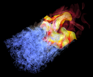
Figure 1. (a) Isosurface of vorticity magnitude ( $\omega = \omega _{max}/30$) coloured by the progress variable
  $c$ and isosurface of
  $c =0.8$ coloured by heat release rate (HRR) for freely propagating planar flames, where
  $\omega _{max}$ is the maximum value of the vorticity magnitude in the domain. The range of
  $c$ is from 0 to 1 and the range of HRR is from 0.4
 $\times 10^{9}$ to 2.0
 $\times 10^{9}\ \textrm {J}\ \textrm {m}^{-3}\ \textrm {s}^{-1}$ for all three cases. The slices show 2-D distributions of the surface density function
  $|\boldsymbol {\nabla }{c}|$. The range of
  $|\boldsymbol {\nabla }{c}|\delta _L$ is from 0 to 0.4 for case
  $L$, to 0.9 for case
  $M$ and to 1.7 for case
  $H$. (b) Three-dimensional rendering of the progress variable
  $c$ and the isosurface of
  $c =0.8$ coloured by HRR for the slot-jet flame. The range of
  $c$ is from 0 to 1 and the range of HRR is from 0 to
  $1.9\times 10^{9}\ \textrm {J}\ \textrm {m}^{-3}\ \textrm {s}^{-1}$.
The simulations were initialized with a corresponding laminar premixed flame solution and a homogeneous isotropic turbulence field based on a prescribed Passot–Pouquet energy spectrum (Passot & Pouquet Reference Passot and Pouquet1987). Three cases, i.e. case  $L$, case
  $M$ and case
  $H$, with different turbulent intensities were considered, where ‘
 $L$’, ‘
 $M$’ and ‘
 $H$’ refer to the level of turbulence (low, medium and high). The simulation parameters are listed in table 1, where
  $l_t$ is the turbulence integral length scale,
  $u'$ is the turbulent velocity and
  $\tau _e$ is the eddy turn-over time. The ratio of the turbulence integral length scale to flame thickness,
  $l_t/\delta _L$, is 1.0, which is of similar order as that found in a slot burner flame (Sankaran et al. Reference Sankaran, Hawkes, Chen, Lu and Law2007) and in a recent highly turbulent jet flame (Wang et al. Reference Wang, Hawkes, Chen, Zhou, Li and Aldén2017b). The turbulent Reynolds number is defined as
  $Re = u'l_t/\nu$, where
  $\nu$ is the viscosity. The Karlovitz number is defined as
  $Ka = \tau _L/\tau _\eta$, where
  $\tau _\eta = (\nu l_t/u'^{3})^{1/2}$ is the Kolmogorov time scale. In the Peters regime diagram (Peters Reference Peters2000), case
  $L$ is located in the thin reaction zones regime, while case
  $M$ and case
  $H$ are in the broken reaction zones regime. A linear forcing method was employed (Carroll & Blanquart Reference Carroll and Blanquart2016) to maintain a statistically stationary turbulent flame. The turbulent forcing was applied everywhere except for the boundaries in the streamwise direction to prevent the interaction of forcing with the inflow/outflow physical boundaries. Note that both of the forcing and flames were initialized at the beginning of the DNS. The flames reach a statistically steady state after the initial period, and statistical results presented in the paper are collected when the flames are statistically steady. It is found that turbulence parameters such as turbulent kinetic energy do not vary much in the vicinity of the flames compared with those in the upstream of the flames. Therefore, the interactions of turbulence and the flames could be characterized using the turbulence parameters in the reactants.
Table 1. Simulation parameters of the planar flames.

The computational domain is  $L_x \times L_y \times L_z = 6L \times L \times L$ in the streamwise direction
  $x$ and lateral directions
  $y$ and
  $z$, respectively, where
  $L$ is 3.14 mm. The grid resolution is chosen to properly resolve all the flame and turbulence scales. Uniform grids were used in all directions and the number of grids is
  $N_x \times N_y \times N_z = 768 \times 128 \times 128$ for case
  $L$ and case
  $M$ with a grid size of
  $24.5\ \mathrm {\mu }\textrm {m}$. In order to resolve the small-scale turbulence structures of case
  $H$, the grid number is increased to
  $N_x \times N_y \times N_z = 1344 \times 224 \times 224$ with a grid size of
  $14.0\ \mathrm {\mu }\textrm {m}$. There is more than 0.5 grid for all cases to resolve the smallest turbulence scale, i.e. the Kolmogorov scale
  $\eta$. Note that the laminar flame thickness is 0.66 mm, so that the DNS grids are sufficient for the flames.
A reduced chemical mechanism for premixed  $\textrm {CH}_4/\textrm {air}$ flames with NO was employed (Lu & Law Reference Lu and Law2008). The reduced mechanism, based on GRI-Mech3.0, contains 268 elementary reactions and 44 species, of which 28 species were transported on the DNS grid. The mechanism has been used and validated in previous DNS studies (Wang et al. Reference Wang, Hawkes, Chen, Zhou, Li and Aldén2017b). Constant species Lewis numbers (Le), determined from a fit to mixture-averaged transport properties in a premixed flame, were employed for transport properties (Wang et al. Reference Wang, Hawkes, Chen, Zhou, Li and Aldén2017b).
2.2. Slot-jet premixed flames
The configuration of the slot-jet flame consists of a coflow and a central jet (figure 1b). The coflow of the DNS is generated from lean  $\textrm {C}_3\textrm {H}_8/\textrm {air}$ combustion with an equivalence ratio of 0.87, and the coflow temperature is 1500 K. The thermochemical conditions of the central jet are determined by adiabatically mixing the coflow and a cold jet (
 $\textrm {C}_2\textrm {H}_4/\textrm {air}$ mixture with a temperature of 300 K and an equivalence ratio of 1.2). The resultant equivalence ratio of the central jet,
  $\phi _j$, is 1.07. The temperature of the central jet,
  $T_j$, is 823 K. This DNS case is denoted as ‘case
  $J$’.
$J$’.
The jet velocity  $U_j$ is
  $163\ \textrm {m}\ \textrm {s}^{-1}$ and the coflow velocity
  $U_c$ is
  $7.6 \ \textrm {m}\ \textrm {s}^{-1}$. The mean velocity profile at the inlet is given as
 \begin{equation} U = U_j+\frac{U_c-U_j}{2}\left[1+\tanh\left(\frac{y-H/2}{\delta}\right)\tanh\left(\frac{y+H/2}{\delta}\right)\right], \end{equation}
where the jet width  $H$ is 1.5 mm, and the shear layer thickness
  $\delta$ is specified as 0.1
 $H$. The jet Reynolds number based on
  $U_j$ and
  $H$ is
  $Re_j =2880$. The profile of a scalar
  $\psi$ (temperature or species mass fractions) at the inlet is similar to that in Wang et al. (Reference Wang, Hawkes, Chen, Zhou, Li and Aldén2017b) with a smooth transition between the jet and the coflow. A turbulence field is obtained by generating an auxiliary homogeneous isotropic turbulence. The turbulent velocity
  $u'$ is 10 % of
  $U_j$ for both cases and the integral length scale
  $l_t$ is the same as
  $H$, i.e. 1.5 mm. The isotropic turbulence field is then filtered outside of the jet and added to the mean inlet velocity using Taylor's hypothesis. The other simulation parameters are listed in table 2.
Table 2. Simulation parameters of the slot-jet flame.
The computational domain is  $L_x\times L_y\times L_z = 60H \times 40H \times 10H$ in the streamwise
  $x$, traverse
  $y$ and spanwise
  $z$ directions, respectively. The grid spacing is chosen to resolve the flame and turbulence structures. Particularly, a uniform grid with
  $\Delta x = 50\ \mathrm {\mu }\textrm {m}$ and
  $\Delta z = 37.5\ \mathrm {\mu }\textrm {m}$ is used in the streamwise and spanwise directions, respectively. A stretched grid is used in the
  $y$ direction with
  $\Delta y = 37.5\ \mathrm {\mu }\textrm {m}$ in the region between
  $y/H = -5$ and 5, and gradually stretched outside of this region. There is at least 0.5 grid point across the Kolmogorov scale,
  $\eta$, throughout the computational domain, satisfying the criterion for resolving turbulence scales. The resultant number of grids is
  $N_x\times N_y\times N_z = 1800 \times 800 \times 400$. The boundary conditions are periodic in the spanwise direction and non-reflecting in other directions.
A reduced mechanism for  $\textrm {C}_2\textrm {H}_4$ combustion including 206 elementary reactions and 32 species was used (Luo et al. Reference Luo, Yoo, Richardson, Chen, Law and Lu2012). This mechanism has been validated for various problems including autoignition and premixed flame propagation. The simulations were advanced for 3
 $\tau _j$ after reaching a statistically steady state, where
  $\tau _j$ is the flow-through time estimated as
  $\tau _j = L_x/U_j$.
2.3. DNS solver
In all simulations, the DNS code S3D (Chen et al. Reference Chen2009) was employed to solve the compressible transport equations for continuity, momentum, species mass fractions and total energy. The code uses a fourth-order Runge–Kutta method for time integration and a skew-symmetric, eighth-order explicit finite difference spatial scheme (Kennedy & Carpenter Reference Kennedy and Carpenter1994; Kennedy, Carpenter & Lewis Reference Kennedy, Carpenter and Lewis2000). A tenth-order filter was applied every 10 time steps to damp high-wavenumber oscillations. Improved Navier–Stokes characteristic boundary conditions (known as NSCBC) were used to prescribe the inflow and outflow boundary conditions (Yoo & Im Reference Yoo and Im2007).
3. Mathematical background
3.1. The coordinate system
We consider a flame element in a coordinate system described in figure 2. The flame normal vector is denoted as  $\boldsymbol {n}$, which is calculated as
 \begin{equation} {\boldsymbol{n}} ={-}\boldsymbol{\nabla}{c}/|\boldsymbol{\nabla}{c}|, \end{equation}
where  $c$ is the progress variable based on mass fractions of
  $\textrm {O}_2$ for freely propagating planar flames and
  $\textrm {H}_2\textrm {O}$ for the slot-jet flame. The value of
  $c$ increases monotonically from zero in the reactants to unity in the products. Sensitivity analyses of the results based on different definitions of the progress variable were carried out by Wang et al. (Reference Wang, Hawkes and Chen2017a) for understanding high
  $Ka$ flame structures and by Lipatnikov et al. (Reference Lipatnikov, Sabelnikov, Hernández-Pérez, Song and Im2020) for flamelet modelling of turbulent premixed flames with various
  $Ka$. In general, the selection of species for calculating the progress variable does not have significant impact on the trends of the results reported in these studies, though quantitative difference was observed. In the present work, we focus on the statistics of various quantities related to flame stretch and turbulence–flame interactions, with the results being little affected by this selection.

Figure 2. Schematic of the coordinate system.
By definition, the flame normal vector points towards the reactants. In a 3-D coordinate system, the flame normal vector could be rewritten as  ${\boldsymbol {n}} = {\boldsymbol {n}}(n_x, n_y, n_z)$, where
  $n_x$,
  $n_y$ and
  $n_z$ are components of the flame normal vector. In 2-D analysis, the
  $x$–
$x$– $y$ plane is taken as the measuring plane unless otherwise specified, where velocities and scalars such as progress variable and species mass fractions can be accessed in the plane. No information in the
  $z$ direction is used. Note that the mean direction of flame propagation aligns with
  $x$ for freely propagating planar flames, while it mostly aligns with
  $y$ for the slot-jet flame, so the
  $x$–
$x$– $y$ plane captures properly the mean behaviour of the flames. The projection of the flame normal vector in the measuring plane is
  ${\boldsymbol {n}}^{p}_{xy}$ with
  ${\boldsymbol {n}}^{p}_{xy} = {\boldsymbol {n}}^{p}_{xy}(n_x, n_y)$ which is unknown from planar measurement, and the unit vector normal to the flame front in the measuring plane is
  ${\boldsymbol {n}}_{xy}$ with
  ${\boldsymbol {n}}_{xy} = {\boldsymbol {n}}_{xy}(n_{x, xy}, n_{y, xy})$ which could be measured with planar images.
The in-plane angle  $\theta$ is defined as the angle between
  ${\boldsymbol {n}}^{p}_{xy}$ and the axis of
  $y$, i.e.
  $\theta = \arctan 2(n_x, n_y)$, and the out-of-plane angle
  $\phi$ is defined as the angle between
  ${\boldsymbol {n}}$ and the
  $x$–
$x$– $y$ plane, i.e.
  $\phi = \arcsin (n_z)$. The angle
  $\theta$ is known from planar measurement and satisfies
  $-{\rm \pi} \leqslant \theta \leqslant {\rm \pi}$, while the angle
  $\phi$ is unknown from planar measurement and is in the range of
  $-{\rm \pi} /2 \leqslant \phi \leqslant {\rm \pi}/2$. Based on these notations, it is obvious that the most probable values of (
 $\theta , \phi$) should be roughly (
 $-{\rm \pi} /2, 0$) for freely propagating planar flames and (
 $-{\rm \pi}$ or
  ${\rm \pi} , 0$) for the slot-jet flame, if we only consider the flame branch with
  $y > L_y/2$ and neglect the shear layer effect. For an isotropic distribution of a unit vector, the PDFs of
  $\theta$ and
  $\phi$ can be written as (Veynante et al. Reference Veynante, Lodato, Domingo, Vervisch and Hawkes2010b; Wang et al. Reference Wang, Hawkes and Chen2016)
 \begin{gather} P_{\theta}(\theta) = 1/2{\rm \pi}, \end{gather}
 \begin{gather}P_{\phi}(\phi) = \cos\phi/2. \end{gather}
3.2. The calculation of 2-D and 3-D flame stretch
The methods for 2-D and 3-D estimations of flame stretch and its related quantities are explained. Equation (1.1) can be recast into
 \begin{equation} \frac{\delta\dot{A}}{\delta{A}} = (\delta_{ij}-n_in_j)\frac{\partial\dot{X}_i}{\partial{x}_j} = a_t + S_d(\boldsymbol{\nabla}\boldsymbol{\cdot}\boldsymbol{n}), \end{equation}
where  $a_t$ is the flame tangential strain rate and
  $\boldsymbol {\nabla }\boldsymbol {\cdot }\boldsymbol {n}$ is the flame curvature. It is obvious that the flame curvature, tangential strain rate and displacement velocity are key quantities that determine the flame stretch. Therefore, these flame stretch-related quantities will be examined in detailed. The tangential strain rate,
  $a_t$, is calculated as
 \begin{equation} a_t = \boldsymbol{\nabla}\boldsymbol{\cdot}{\boldsymbol{u}} - a_n, \end{equation}
where  $\boldsymbol {\nabla }\boldsymbol {\cdot }\boldsymbol {u}$ is the dilatation and
  $a_n$ is the normal strain rate calculated as
 \begin{equation} a_n = n_iS_{ij}n_j, \end{equation}
where  $S_{ij}$ is the strain rate tensor component defined as
 \begin{equation} S_{ij} = (\partial{u}_i/\partial{x}_j+\partial{u}_i/\partial{x}_i)/2. \end{equation}
 The transport equation of the progress variable  $c$ is
 \begin{equation} \rho\frac{\textrm{D}c}{\textrm{D}t} = \dot{\omega}_c + \frac{\partial}{\partial{x_i}} \left(\rho{D}_c\frac{\partial{c}}{\partial{x_i}}\right), \end{equation}
where  $\dot {\omega }_c$ is the reaction rate of the progress variable and
  $D_c$ is the diffusivity of the progress variable. The progress variable isosurface propagates at a speed of
  $S_d$, which can be estimated as
  $S_{d} = S_a - {\boldsymbol {u}}\boldsymbol {\cdot }{\boldsymbol {n}}$ (Poinsot & Veynante Reference Poinsot and Veynante2005), where
  $S_a$ is the absolute velocity of the flame. In the practice of DNS,
  $S_d$ is calculated as (Wang et al. Reference Wang, Hawkes and Chen2017a,Reference Wang, Hawkes, Chen, Zhou, Li and Aldénb)
 \begin{equation} S_d = \frac{1}{|\boldsymbol{\nabla}{c}|}\frac{\textrm{D}c}{\textrm{D}t} = \frac{\dot{\omega}_c}{\rho|\boldsymbol{\nabla}{c}|} + \frac{1}{\rho|\boldsymbol{\nabla}{c}|}\frac{\partial}{\partial{x_i}}\left(\rho{D}_c\frac{\partial{c}}{\partial{x_i}}\right). \end{equation}
 The 2-D estimation of various quantities in the  $x$–
$x$– $y$ plane is discussed. The 2-D curvature is denoted as
 \begin{equation} (\boldsymbol{\nabla}\boldsymbol{\cdot}{\boldsymbol{n}})_{2D} = \frac{\partial{n}_{x,xy}}{\partial{x}} + \frac{\partial{n}_{y,xy}}{\partial{y}}. \end{equation}
The 2-D tangential strain rate  $a_{t,2D}$ is estimated as
 \begin{equation} a_{t,2D} = (\boldsymbol{\nabla}\boldsymbol{\cdot}{\boldsymbol{u}})_{2D} - a_{n,2D}, \end{equation}
where  $(\boldsymbol {\nabla }\boldsymbol {\cdot }{\boldsymbol {u}})_{2D}$ is the 2-D dilatation in the
  $x$–
$x$– $y$ plane computed as
 \begin{equation} (\boldsymbol{\nabla}\boldsymbol{\cdot}{\boldsymbol{u}})_{2D} = \frac{\partial{u}}{\partial{x}} + \frac{\partial{v}}{\partial{y}}. \end{equation}
The quantity  $a_{n,2D}$ is the 2-D normal strain rate in the
  $x$–
$x$– $y$ plane with
 \begin{equation} a_{n,2D} = {n}_{i,xy}S_{ij,xy}{n}_{j,xy}, \end{equation}
where  $S_{ij,xy}$ is the strain rate tensor component in the
  $x$–
$x$– $y$ plane.
The 2-D displacement velocity  $S_{d,2D}$ can be measured experimentally as
  $S_{d,2D} = S_{a,xy} - {\boldsymbol {u}}_{xy}\boldsymbol {\cdot }{\boldsymbol {n}}_{xy}$ (Hartung et al. Reference Hartung, Hult, Balachandran, MacKley and Kaminski2009), where
  $S_{a,xy}$ is the absolute velocity of the flame and
  ${\boldsymbol {u}}_{xy}$ is the 2-D flow velocity in the
  $x$–
$x$– $y$ plane. By accounting for the out-of-plane fluid motion, it is estimated in the DNS by the following apparent relationship (Hartung et al. Reference Hartung, Hult, Balachandran, MacKley and Kaminski2009; Chakraborty et al. Reference Chakraborty, Hartung, Katragadda and Kaminski2011; Hawkes et al. Reference Hawkes, Sankaran and Chen2011):
 \begin{equation} S_{d,2D} = S_d/\cos\phi. \end{equation}
 The 2-D flame stretch can be, therefore, computed as  $a_{t,2D} + S_{d,2D}(\boldsymbol {\nabla }\boldsymbol {\cdot }{\boldsymbol {n}})_{2D}$.
3.3. Statistical tools
The analysis in this paper employs surface averaged quantities. The fine-grained flame surface density  $\varSigma ^{*}$ is defined as (Veynante & Vervisch Reference Veynante and Vervisch2002)
 \begin{equation} \varSigma^{*} = \overline{|\boldsymbol{\nabla}{c}|\delta(c - c^{*})}, \end{equation}
where  $|\boldsymbol {\nabla }{c}|$ is the surface density function and
  $\delta$ is the delta function. The operation
  $\overline {(\cdot )}$ denotes ensemble average. The fine-grained surface average of a quantity
  $Q$ is denoted as
 \begin{equation} \left\langle{Q}\right\rangle_s^{*} = \frac{\overline{Q|\boldsymbol{\nabla}{c}|\delta(c - c^{*})}}{\varSigma^{*}}. \end{equation}
The flame stretch and the related quantities are averaged on the isosurface of the progress variable  $c = c^{*}$, so that the results depend on the choice of
  $c^{*}$. The generalized flame surface density
  $\varSigma$ has been introduced to overcome this problem (Borger et al. Reference Borger, Veynante, Boughanem and Trové1998; Veynante & Vervisch Reference Veynante and Vervisch2002; Chakraborty & Cant Reference Chakraborty and Cant2004), which is obtained by integrating (3.15) over all isosurface levels,
 \begin{equation} \varSigma = \int_0^{1} \varSigma^{*}\,\textrm{d}c^{*} = \int_0^{1} \overline{|\boldsymbol{\nabla}{c}|\delta(c - c^{*})}\,\textrm{d}c^{*} = \overline{|\boldsymbol{\nabla}{c}|}. \end{equation}
The generalized surface average of  $Q$ is denoted as
 \begin{equation} \left\langle{Q}\right\rangle_s = \frac{\overline{Q|\boldsymbol{\nabla}{c}|}}{\varSigma}. \end{equation}
 Statistics such as PDF and joint PDF are also explored to reveal the difference between 2-D and 3-D flame stretch and the related quantities. Consistent with the generalized surface average, the PDF and joint PDF are also weighted by  $|\boldsymbol {\nabla }{c}|$. In order to exclude regions where reaction is unimportant, the results are conditioned on
  $0.3 \leqslant {c} \leqslant {0.9}$.
3.4. Models for converting 2-D to 3-D statistics
We derive models to convert statistics of a flame stretch-related quantity  $\psi$ from 2-D measurements to 3-D reality, assuming isotropy of the flame normal vector orientation. Particularly, the aim is to use the 2-D surface averaged quantity
  $\langle {\psi _{2D}}\rangle _s$ to obtain
  $\langle {\psi }\rangle _{s,M}$, and to use the 2-D PDF
  $P_{\psi ,{2D}}(\psi _{2D})$ to obtain
  $P_{\psi ,M}(\psi )$, where the subscript ‘
 $M$’ indicates a specific model.
3.4.1. Tangential strain rate model
Following the notations of Hawkes et al. (Reference Hawkes, Sankaran and Chen2011), the 3-D tangential strain rate can be written as
 \begin{equation} a_t = \frac{\partial{u_{t1}}}{\partial{x_{t1}}} + \frac{\partial{u_{t2}}}{\partial{x_{t2}}}, \end{equation}
where  $t_1$ is tangent to the flame that also lies in the measuring plane and
  $t_2$ is the flame tangent perpendicular to
  $t_1$. Now the 2-D tangential strain rate in the measuring plane is
 \begin{equation} a_{t1,2D} = \frac{\partial{u_{t1}}}{\partial{x_{t1}}} \end{equation}
while the 2-D out-of-plane tangential strain rate is
 \begin{equation} a_{t2,2D} = \frac{\partial{u_{t2}}}{\partial{x_{t2}}}. \end{equation}
Two assumptions will be developed: the first is that  $a_{t1,2D} = a_{t2,2D}$; the second is that
  $a_{t1,2D}$ and
  $a_{t2,2D}$ are statistically independent. Both assumptions lead to the following relationship of 2-D and 3-D surface averaged tangential strain rate:
 \begin{equation} \left\langle{a_t}\right\rangle_{s,M} = 2\langle{a_{t,2D}}\rangle_s. \end{equation}
If  $a_{t1,2D} = a_{t2,2D}$, the 2-D PDF is related to the 3-D one by
 \begin{equation} P_{a_t,M1}(a_t) = \tfrac{1}{2}P_{a_{t,2D}}\left(\tfrac{1}{2}a_{t}\right). \end{equation}
If we assume that  $a_{t1,2D}$ and
  $a_{t2,2D}$ are statistically independent, the PDF of their sum is the convolution of their PDFs,
 \begin{equation} P_{a_t,M2}(a_t) = \int_{-\infty}^{\infty}P_{a_{t1,2D}}(a_{t1})P_{a_{t2,2D}}(a_t - a_{t1})\,\textrm{d}a_{t1}. \end{equation}
Because of isotropy, the statistics of  $a_{t1}$ and
  $a_{t2}$ are identical, i.e.
  $P_{a_{t1,2D}} = P_{a_{t2,2D}}$, so that
 \begin{equation} P_{a_t,M2}(a_t) = \int_{-\infty}^{\infty}P_{a_{t1,2D}}(a_{t1})P_{a_{t1,2D}}(a_t - a_{t1})\,\textrm{d}a_{t1}. \end{equation}
3.4.2. Curvature model
From Hawkes et al. (Reference Hawkes, Sankaran and Chen2011), the curvature measured in 2-D is related to the 3-D principal curvatures by
 \begin{equation} \cos\phi(\boldsymbol{\nabla}\boldsymbol{\cdot}{\boldsymbol{n}})_{2D} = \kappa_1\cos^{2}\alpha + \kappa_2\sin^{2}\alpha, \end{equation}
where  $\kappa _1$ and
  $\kappa _2$ are the two principal curvatures with the corresponding principal vectors denoted as
  ${\boldsymbol {k}}_1$ and
  ${\boldsymbol {k}}_2$, respectively. The unit vector
  ${\boldsymbol {t}}_1$ is lying in both the measuring plane and the flame tangent plane. Here
  $\alpha$ is the angle between
  ${\boldsymbol {t}}_1$ and
  ${\boldsymbol {k}}_1$. Note that the above relationship is general and no assumptions are made (Hawkes et al. Reference Hawkes, Sankaran and Chen2011). If
  $\phi$ and
  $\alpha$ are not correlated with other variables, the following is obtained:
 \begin{equation} \left\langle{\cos\phi}\right\rangle_s\left\langle{(\boldsymbol{\nabla}\boldsymbol{\cdot}{\boldsymbol{n}})_{2D}}\right\rangle_s = \langle{\kappa_1}\rangle_s\langle{\cos^{2}\alpha}\rangle_s + \langle{\kappa_2}\rangle_s\langle{\sin^{2}\alpha}\rangle_s. \end{equation}
By assuming  $\phi$ and
  $\alpha$ are isotropically distributed, we have
  $\langle {\cos \phi }\rangle _s = {\rm \pi}/4$ and
  $\langle {\cos ^{2}\alpha }\rangle _s = \langle {\sin ^{2}\alpha }\rangle _s = 1/2$. Finally, the following surprisingly simple relationship is obtained:
 \begin{equation} \left\langle{(\boldsymbol{\nabla}\boldsymbol{\cdot}{\boldsymbol{n}})_{2D}}\right\rangle_s = {\rm \pi}/2(\left\langle{\kappa_1}\right\rangle_s + \left\langle{\kappa_2}\right\rangle_s) = 2/{\rm \pi}\left\langle{\boldsymbol{\nabla}\boldsymbol{\cdot}{\boldsymbol{n}}}\right\rangle_s, \end{equation}
where  $\boldsymbol {\nabla }\boldsymbol {\cdot }{\boldsymbol {n}} = \kappa _1 + \kappa _2$ is the 3-D curvature. So that the surface averaged
  $\boldsymbol {\nabla }\boldsymbol {\cdot }{\boldsymbol {n}}$ can be modelled as
 \begin{equation} \left\langle{\boldsymbol{\nabla}\boldsymbol{\cdot}{\boldsymbol{n}}}\right\rangle_{s,M} = {\rm \pi}/2\left\langle{(\boldsymbol{\nabla}\boldsymbol{\cdot}{\boldsymbol{n}})_{2D}}\right\rangle_{s}. \end{equation}
The following model is proposed to approximately the PDF of  $\boldsymbol {\nabla }\boldsymbol {\cdot }{\boldsymbol {n}}$, using that of
  $(\boldsymbol {\nabla }\boldsymbol {\cdot }{\boldsymbol {n}})_{2D}$:
 \begin{equation} P_{\boldsymbol{\nabla}\boldsymbol{\cdot}{\boldsymbol{n}},M}(\boldsymbol{\nabla}\boldsymbol{\cdot}{\boldsymbol{n}}) = \frac{2}{\rm \pi}P_{(\boldsymbol{\nabla}\boldsymbol{\cdot}{\boldsymbol{n}})_{2D}} \left(\frac{2}{\rm \pi}\boldsymbol{\nabla}\boldsymbol{\cdot}{\boldsymbol{n}}\right). \end{equation}
3.4.3. Displacement velocity model
If we assume  $S_d$ and
  $\phi$ are not correlated and using (3.14), the surface averaged
  $S_{d}$ are modelled, using that of
  $S_{d,2D}$, by
 \begin{equation} \langle{S_{d}}\rangle_{s,M} = \langle{S_{d,2D}}\rangle_s\langle{\cos\phi}\rangle_s = {\rm \pi}/4\langle{S_{d,2D}}\rangle_s. \end{equation}
The following model is proposed to connect the PDF of  $S_d$ and that of
  $S_{d,2D}$:
 \begin{equation} P_{S_d,M}(S_d) = \frac{4}{\rm \pi}P_{S_{d,2D}}\left(\frac{4}{\rm \pi}S_{d}\right). \end{equation}
4. Results and discussion
In this section, the general characteristics of various flames are first discussed and the flame normal vector orientations are quantified. Then, the instantaneous and statistical flame stretch-related quantities are explored, and the 2-D and 3-D results are compared. Models for approximating the 3-D results using the 2-D measurements are evaluated. Third, the instantaneous and statistical results of 2-D and 3-D flame stretch are compared and discussed. Finally, the 2-D and 3-D turbulence–flame interactions are examined for various DNS cases, and the discrepancy of turbulence–flame interactions from 2-D and 3-D measurements are highlighted.
4.1. General characteristics
The general characteristics of the DNS cases are discussed. Figure 1(a) shows the isosurface of vorticity magnitude coloured by the progress variable and the isosurface of  $c = 0.8$ coloured by HRR for freely propagating planar flames. Note that
  $c = 0.8$ corresponds to the location of maximum HRR in the corresponding laminar flame. Fine-scale eddies are observed in the reactants and the eddies become fewer and larger behind the flame front, which is due to the thermal expansion effects (Tanahashi, Fujimura & Miyauchi Reference Tanahashi, Fujimura and Miyauchi2000). The intensity of turbulent eddies is increased from case
  $L$ to case
  $H$. For case
  $M$ and case
  $H$ in the broken reaction zones regime, the fine-scale eddies are able to enter into the reaction zone so that the inner flame structures are affected. The distributions of surface density function,
  $|\nabla {c}|$, are also shown for freely propagating planar flames. The surface density function can be regarded as a reciprocal flame thickness (Wang et al. Reference Wang, Hawkes, Chen, Zhou, Li and Aldén2017b). Moreover, it is closely related to the flame surface density as seen in the previous section. Figure 1(a) indicates that with increasing
  $Ka$, the fluctuation of
  $|\boldsymbol {\nabla }{c}|$ becomes more evident. Local thinning of the flame front in case
  $H$ is clearly observed. But on average the flame brush is thicker in case
  $H$ compared with the other two cases. Similar observations were made in a premixed jet flame by Wang et al. (Reference Wang, Hawkes, Chen, Zhou, Li and Aldén2017b).
Figure 1(b) displays 3-D rendering of the progress variable and the isosurface of  $c = 0.8$ coloured by HRR for the slot-jet flame. As can be seen, the HRR is negligible in the near field, where only mixing of the jet and coflow occurs. Evident HRR is observed after
  $x/H = 5$ when autoignition occurs. The magnitude of HRR increases with increasing downstream distance. Wang et al. (Reference Wang, Hawkes and Chen2017a) showed that such enhanced reaction rate in jet-type flames is related to enhanced levels of radicals such as OH and H in the downstream region. There are significant interactions between the shear-generated turbulence and the flame, modifying the flame topology, as will be quantified shortly.
Figure 1 indicates that both the freely propagating planar and slot-jet flames exhibit evident 3-D behaviours. Therefore, the flame orientations are analysed. For the slot-jet flame, three downstream locations, i.e.  $x/H = 10$,
  $20$ and
  $30$, are selected for the analysis. Figure 3 shows the PDFs of the out-of-plane angle
  $\phi$ and the in-plane angle
  $\theta$ for various cases. As can be seen, the distribution of
  $\phi$ is very similar to that predicted using (3.3), implying that the distribution of
  $\phi$ is close to isotropy. This is valid for both flames with and without a mean shear. For freely propagating planar flames, the most probable value of
  $\theta$ is approximately
  $-{\rm \pi} /2$, as expected. The distribution of
  $\theta$ becomes more isotropic with increasing
  $Ka$, due to the influence of intense turbulence. This observation is consistent with previous experimental results (Lee et al. Reference Lee, North and Santavicca1992). A different picture is observed for the slot-jet flame. In particular, the most probable value of
  $\theta$ is approximately
  $-3{\rm \pi} /4$ or
  ${\rm \pi} /4$. This is attributed to the local flame surface convex towards the products due to the presence of mean shear (Wang et al. Reference Wang, Hawkes and Chen2016). Particularly, as will be shown later, the flame normal vector aligns with the most compressive strain rate of the flow, which roughly orients roughly
  $-3{\rm \pi} /4$ or
  ${\rm \pi} /4$ to the radial direction. The results are also consistent with previous studies of passive scalars in non-reacting shear flows (Ashurst et al. Reference Ashurst, Kerstein, Kerr and Gibson1987; Nomura & Elghobashi Reference Nomura and Elghobashi1992). The distribution of
  $\theta$ is more isotropic with increasing downstream distance for the slot-jet flame.

Figure 3. The PDFs of the out-of-plane angle  $\phi$ and the in-plane-angle
  $\theta$ for the (a) freely propagating planar flames and (b) slot-jet flame.
The joint PDFs of out-of-plane angle  $\phi$ and the in-plane angle
  $\theta$ for various cases are shown in figure 4. For both the freely propagating planar and slot-jet flames, the two angles are poorly correlated. Similar results were reported by Veynante et al. (Reference Veynante, Lodato, Domingo, Vervisch and Hawkes2010b) and Wang et al. (Reference Wang, Hawkes and Chen2016). Consequently, the joint PDF of
  $\phi$ and
  $\theta$ could be modelled using the product of their marginal PDFs, i.e.
  $P_{\phi \theta }(\phi , \theta ) = P_{\phi }(\phi )P_{\theta }(\theta )$.

Figure 4. Joint PDFs of out-of-plane angle  $\phi$ and the in-plane angle
  $\theta$ for the (a) freely propagating planar flames and (b) slot-jet flame.
The correlation of  $\phi$ and
  $\theta$ is further demonstrated using the independence function, which is defined as
  $I(\phi , \theta ) = P_{\phi \theta }(\phi , \theta )/P_{\phi }(\phi )/P_{\theta }(\theta )$. Unity values of the independence function indicate that
  $\phi$ and
  $\theta$ are independent. Figure 5 shows the values of
  $I$ in various cases. As can be seen,
  $I$ is close to unity in most regions. There are also regions where
  $I$ is much larger or smaller than unity, the PDF of which is, however, small as seen in figure 4.

Figure 5. Independence functions of out-of-plane angle  $\phi$ and the in-plane angle
  $\theta$ for the (a) freely propagating planar flames and (b) slot-jet flame.
4.2. Evaluation of the models for flame stretch-related quantities
The orientations of the out-of-plane angle  $\phi$ and the in-plane angel
  $\theta$ examined above play significant roles in the relationship between 2-D and 3-D values of flame stretch-related quantities. The assumption of
  $\phi$ being isotropic has also been employed to derive models that convert 2-D to 3-D statistics of flame properties, as demonstrated in § 3.4. Let us now consider the flame stretch-related quantities, i.e. tangential strain rate, curvature and displacement velocity. Figure 6 shows the instantaneous 2-D and 3-D values of these quantities along
  $c = 0.8$ from a typical
  $x$–
$x$– $y$ plane of case
  $M$. As can be seen, the flame front is wrinkled by turbulence. Very large positive curvature is observed in both 2-D and 3-D results, which corresponds to small-scale wrinkling of the flame front. In general, the 3-D values of curvature are higher than the 2-D values along the flame. The 3-D tangential strain rate is also larger than the 2-D one. In contrast, the 3-D displacement velocity is slightly smaller than the 2-D one, as expected from (3.14). It is interesting to see that there is a negative correlation between the displacement velocity and curvature, consistent with Wang et al. (Reference Wang, Hawkes and Chen2017a) for methane–air premixed jet flames.

Figure 6. Comparison of instantaneous 2-D and 3-D values of tangential strain rate  $a_t\tau _L$, curvature
  $(\boldsymbol {\nabla }\boldsymbol {\cdot }{\boldsymbol {n}})\delta _L$ and displacement velocity
  $S_d/S_l$ along
  $c = 0.8$ from a typical slice of case
  $M$.
$M$.
More difference between the 2-D and 3-D values of flame stretch-related quantities is shown, and the performance of models described in § 3.4 is evaluated. Figure 7 compares 2-D, 3-D and model predicted surface averaged tangential strain rate, curvature and displacement velocity for various cases. For freely propagating planar flames, the results are shown across the flame brush as a function of the Favre averaged progress variable  $\tilde {c}$, while for the slot-jet flame, the results along the streamwise direction are presented. As can be seen, the 3-D surface averaged tangential strain rate and curvature are generally larger than their 2-D counterparts, while the 3-D surface averaged displacement velocity is smaller than the 2-D result in magnitude. The model predictions are in overall good agreement with the actual 3-D surface averaged quantities for various cases.

Figure 7. Comparison of 2-D, 3-D and model predicted surface averaged tangential strain rate  $a_t\tau _L$, curvature
  $(\boldsymbol {\nabla }\boldsymbol {\cdot }{\boldsymbol {n}})\delta _L$ and displacement velocity
  $S_d/S_l$ across the flame brush of case
  $L$, case
  $M$ and case
  $H$ and along the streamwise direction of case
  $J$.
$J$.
It is crucial to predict accurately the PDFs for flame stretch-related quantities. Figure 8 shows the 2-D, 3-D and model predicted PDFs of the tangential strain rate for various cases. Three representative axial locations of case  $J$ are selected for the analysis. The model based on (3.23) is labelled as ‘M1’ and that based on (3.24) is labelled as ‘M2’. Several observations can be made. First, the range of tangential strain rate is broadened with increasing
  $Ka$ in freely propagating planer flames, which is due to the large straining induced in highly turbulent flames. Second, the tangential strain rate in the slot-jet flame is decreased with downstream distance, in line with the decaying of the jet. Third, the prediction of M2 is in excellent agreement with the actual 3-D PDF, although the peak is over predicted at
  $x/H = 10$ of case
  $J$. Comparatively, the prediction of M1 is less accurate than M2.

Figure 8. Comparison of 2-D, 3-D and model predicted PDFs of tangential strain rate for various cases.
To provide quantitative measures of the performance of the modelled PDFs, a Kullack–Leibler divergence is introduced (Kullback & Leibler Reference Kullback and Leibler1951). The Kullack–Leibler divergence from the actual 3-D PDF,  $P_{a_t}$, to the modelled 3-D PDF,
  $P_{a_t,M}$, is defined as
 \begin{equation} D_{KL} = \sum_{x\in{X}}P_{a_t}(x)\log\left(\frac{P_{a_t}(x)}{P_{a_t,M}(x)}\right), \end{equation}
where  $X$ is the probability space of the tangential strain rate. The Kullack–Leibler divergence measures how one PDF is different from a second. A zero value of
  $D_{KL}$ indicates that the two PDFs are identical. The results of the Kullack–Leibler divergence for various cases are shown in figure 9. It is observed that the values of
  $D_{KL}$ for M2 are lower than those for M1 in all cases, which confirms that M2 is more accurate than M1.

Figure 9. Results of the Kullack–Leibler divergence for the tangential strain rate with different 3-D PDF models in the (a) freely propagating planar flames and (b) slot-jet flame.
The PDFs of curvature are compared in figure 10. For reference, the curvature measured in the  $y$–
$y$– $z$ plane is also displayed. It can be seen that the curvature PDFs from the
  $x$–
$x$– $y$ plane and the
  $y$–
$y$– $z$ plane almost overlap in various cases. Some minor difference is observed in case
  $L$, where the peak value of the curvature PDF in the
  $x$–
$x$– $y$ plane is larger than that in the
  $y$–
$y$– $z$ plane. The 3-D curvature distributions are wider than their 2-D counterparts. The model based on (3.30) is performing reasonably well in all cases.

Figure 10. Comparison of 2-D, 3-D and model predicted PDFs of curvature for various cases.
Finally, the 2-D, 3-D and modelled PDFs of displacement velocity are compared in figure 11. Negative displacement velocity is observed in various cases, which has been reported in previous DNS studies (Chakraborty et al. Reference Chakraborty, Hartung, Katragadda and Kaminski2011; Sankaran et al. Reference Sankaran, Hawkes, Yoo and Chen2015; Wang et al. Reference Wang, Hawkes and Chen2017a). The range of displacement velocity is broadened as turbulent intensity increases in freely propagating planer flames. As can be seen, the model prediction based on (3.32) is in very good agreement with the actual 3-D PDF for all cases.

Figure 11. Comparison of 2-D, 3-D and model predicted PDFs of displacement velocity for various cases.
4.3. Flame stretch
In this section, the 2-D and 3-D flame stretch results are presented. Figure 12 shows the instantaneous 2-D and 3-D values of flame curvature, tangential strain rate, curvature stretch and total flame stretch along  $c = 0.8$ from a typical
  $x$–
$x$– $y$ plane of case
  $M$. Note that flame stretch consists of tangential strain rate and curvature stretch. It has been shown previously that tangential strain rate tends to produce flame surface area while curvature stretch tends to destroy it (Candel & Poinsot Reference Candel and Poinsot1990; Wang et al. Reference Wang, Hawkes, Chen, Zhou, Li and Aldén2017b; Luca et al. Reference Luca, Attili, Lo, Creta and Bisetti2019). This is also true for the current DNS flames. Figure 12 indicates that the mean tangential strain rate is positive and the mean curvature stretch is negative. In general, the 2-D flame stretch and its components are smaller than their 3-D counterparts.

Figure 12. Comparison of instantaneous 2-D and 3-D values of curvature  $(\boldsymbol {\nabla }\boldsymbol {\cdot }{\boldsymbol {n}})\delta _L$, tangential strain rate
  $a_t\tau _L$ and curvature stretch
  $S_d(\boldsymbol {\nabla }\boldsymbol {\cdot }{\boldsymbol {n}})\tau _L$ and total flame stretch
  $a_t\tau _L+S_d(\boldsymbol {\nabla }\boldsymbol {\cdot }{\boldsymbol {n}})\tau _L$ along
  $c = 0.8$ from a typical slice of case
  $M$.
$M$.
There is evident correlation between flame stretch and curvature as shown in figure 12. In order to further assess the correlation, the joint PDFs of flame stretch and curvature for freely propagating planar flames are shown in figure 13. Both the 2-D and 3-D results are displayed. It is clearly observed that the flame stretch is positive in regions with low curvature magnitudes, and highly negative flame stretch occurs in regions with large curvature, the sign of the curvature being unimportant. It is, therefore, concluded that flame area tends to be produced in low curvature regions while it is destroyed in high curvature regions. This is consistent with the results reported in (Wang et al. Reference Wang, Hawkes, Chen, Zhou, Li and Aldén2017b). With increasing levels of turbulence from case  $L$ to case
  $H$, the magnitude of flame stretch also increases. It is interesting to see that although the magnitudes of flame stretch and curvature are smaller in the 2-D results, the trends of the relationship between flame stretch and curvature are reasonably captured. That is, flame stretch is positive (negative) in low (high) curvature regions.

Figure 13. Joint PDFs of (a) 3-D and (b) 2-D flame stretch and curvature for case  $L$, case
  $M$ and case
  $H$.
$H$.
The joint PDFs of flame stretch and curvature at three locations of the slot-jet flame are shown in figure 14. The existence of mean shear does not alter the correlations between flame stretch and curvature qualitatively. More specifically, the observations made above for freely propagating planar flames are also valid for the slot-jet flame. The flame stretch generally decreases with downstream distance, until the reactant is consumed completely and the flame disappears.

Figure 14. Joint PDFs of (a) 3-D and (b) 2-D flame stretch and curvature for various locations of case  $J$.
$J$.
4.4. Turbulence–flame interactions
The turbulence–flame interactions are examined in terms of the flame normal strain rate  $a_n$ and its related terms. Both the 2-D and 3-D results are presented. The flame normal strain rate is also written as
  $n_iS_{ij}n_j$, which was used in the calculation of tangential strain rate (3.5) and flame stretch. According to Wang et al. (Reference Wang, Hawkes and Chen2016),
  $a_n$ can be recast as
 \begin{equation} a_n = n_iS_{ij}n_j = \lambda_1|{\boldsymbol{n}}\boldsymbol{\cdot}{\boldsymbol{e}}_1|^{2} + \lambda_2|{\boldsymbol{n}}\boldsymbol{\cdot}{\boldsymbol{e}}_2|^{2} + \lambda_3|{\boldsymbol{n}}\boldsymbol{\cdot}{\boldsymbol{e}}_3|^{2}, \end{equation}
where  $\lambda _1$,
  $\lambda _2$ and
  $\lambda _3$ are the three principal eigenvalues of the velocity gradient tensor
  $\partial {u_i}/\partial {x_j}$ by the convention
  $\lambda _1 \geqslant \lambda _2 \geqslant \lambda _3$, which are determined from the characteristic equation of
  $\partial {u_i}/\partial {x_j}$ as follows:
 \begin{equation} \lambda^{3}+P\lambda^{2}+Q\lambda+R=0 \end{equation}
with the invariants specified as  $P = -S_{ii}$,
  $Q = (P^{2} - S_{ij}S_{ji} - W_{ij}W_{ji}) / 2$ and
  $R = (-P^{3} + 3PQ - S_{ij}S_{jk}S_{ki} - 3W_{ij}W_{jk}S_{ki}) /3$, where
  $W_{ij} = (\partial {u}_i/\partial {x}_j - \partial {u}_j/\partial {x}_i) / 2$ is the rotation tensor.
The eigenvectors of  $\lambda _1$,
  $\lambda _2$ and
  $\lambda _3$ are
  ${\boldsymbol {e}}_1$,
  ${\boldsymbol {e}}_2$ and
  ${\boldsymbol {e}}_3$, respectively. The orientations of the flame normal vector relative to the principal strain rate directions are characterized by the absolute value of the cosine of the angle between the flame normal vector and the strain rate eigenvectors, i.e.
  $|{\boldsymbol {n}}\boldsymbol {\cdot }{\boldsymbol {e}}_i|$. Note that in 2-D measurements, only the most extensive strain rate
  $\lambda _{1,xy}$ and the most compressive strain rate
  $\lambda _{3,xy}$ are available, while the intermediate strain rate
  $\lambda _{2,xy}$ is absent. Accordingly, only
  $|{\boldsymbol {n}}_{xy}\boldsymbol {\cdot }{\boldsymbol {e}}_{1,xy}|$ and
  $|{\boldsymbol {n}}_{xy}\boldsymbol {\cdot }{\boldsymbol {e}}_{3,xy}|$ are evaluated for the alignment between the flame normal vector and principal strain rates, while
  $|{\boldsymbol {n}}_{xy}\cdot {\boldsymbol {e}}_{2,xy}|$ is not available.
Figure 15 shows the PDFs of the principal strain rates for various cases. As can be seen, the most extensive strain rate of the 3-D results is always positive while the most compressive strain rate is negative. The most probable value of the intermediate strain rate is close to zero, and its distribution is positively skewed. The magnitude of the principal strain rates increases with  $Ka$ for freely propagating planar flames and decreases with downstream distance for the slot-jet flame, as expected. The principal strain rates of 2-D measurements are also shown. The profiles of
  $\lambda _{1,xy}$ and
  $\lambda _{3,xy}$ are very similar to those of
  $\lambda _1$ and
  $\lambda _3$. However, the most extensive (compressive) strain rate of 2-D measurements can be negative (positive). It is concluded that the above behaviours of the 2-D and 3-D principal strain rates are valid in flames with and without a mean shear. The distributions of the 2-D principal strain rates have been measured experimentally by Hartung et al. (Reference Hartung, Hult, Kaminski, Rogerson and Swaminathan2008) in premixed ethylene–air flames stabilized on a bluff body, and qualitatively similar PDFs of the 2-D principal strain rates were reported (see Hartung et al. (Reference Hartung, Hult, Kaminski, Rogerson and Swaminathan2008), figure 10).

Figure 15. The 2-D and 3-D PDFs of principal strain rates for various cases.
The orientation between the flame normal vector and the principal strain rate determines whether the scalar gradient  $|\boldsymbol {\nabla }{c}|$ are produced or destroyed by turbulence (Chakraborty & Swaminathan Reference Chakraborty and Swaminathan2007; Kim & Pitsch Reference Kim and Pitsch2007; Sponfeldner et al. Reference Sponfeldner, Boxx, Beyrau, Hardalupas, Meier and Taylor2015; Wang et al. Reference Wang, Hawkes and Chen2016). Previous investigations of turbulence–scalar interaction in non-reacting flows with and without a mean shear showed a preferential alignment of scalar gradient vector with the most compressive principal strain rate (Ashurst et al. Reference Ashurst, Kerstein, Kerr and Gibson1987). The effects of chemical reactions on the alignment characteristics have been studied in (Swaminathan & Grout Reference Swaminathan and Grout2006; Chakraborty & Swaminathan Reference Chakraborty and Swaminathan2007; Kim & Pitsch Reference Kim and Pitsch2007; Cifuentes et al. Reference Cifuentes, Dopazo, Martin and Jimenez2014), where it was found that the scalar gradient aligns with the most extensive strain rate and turbulence dissipates the scalar gradient in high
  $Da$ flames. This is because in high
  $Da$ flames the dilatation induced by heat release is dominant over the turbulent strain rate. The turbulence–flame interactions of high
  $Ka$ flames were investigated by Wang et al. (Reference Wang, Hawkes and Chen2016) and it was concluded that consistent with non-reacting flows, the scalar gradient aligns with the most compressive strain rate and turbulence generates the scalar gradient. In the present work, the alignment behaviours of the flame normal vector and the principal strain rates are examined in both 2-D and 3-D measurements. Figure 16 shows the distributions of the progress variable in a typical slice of case
  $L$, which is superimposed with the eigenvector of the most extensive and compressive strain rate of 2-D measurements, i.e.
  ${\boldsymbol {e}}_{1,xy}$ and
  ${\boldsymbol {e}}_{3,xy}$. There is a clear preferential alignment between
  ${\boldsymbol {e}}_{3,xy}$ and
  ${\boldsymbol {n}}_{xy}$, while the alignment characteristics between
  ${\boldsymbol {e}}_{1,xy}$ and
  ${\boldsymbol {n}}_{xy}$ are less obvious. This observation is further quantified below.

Figure 16. Distributions of the progress variable in a typical slice of case  $L$: (a) the arrows show the eigenvector of the 2-D most extensive strain rate and (b) the arrows show the eigenvector of the 2-D most compressive strain rate. The black line shows the isoline of
  $c = 0.8$.
The PDFs of  $|{\boldsymbol {n}}\boldsymbol {\cdot }{\boldsymbol {e}}_{i}|$ and
  $|{\boldsymbol {n}}_{xy}\boldsymbol {\cdot }{\boldsymbol {e}}_{i,xy}|$ for case
  $L$ are shown in figure 17. The PDFs for other cases have also been extracted and they are very similar to those of case
  $L$, so that only the results of case
  $L$ are presented. In the 3-D statistics, the flame normal vector aligns preferentially with the most compressive strain rate and misaligns with the most extensive and intermediate strain rates, which is the general feature of high
  $Ka$ (low
  $Da$) flames (Wang et al. Reference Wang, Hawkes and Chen2016). In the 2-D statistics, the alignment of the flame normal vector and the most compressive strain rate is much stronger than its 3-D counterpart. Interestingly, the most probable value of
  $|{\boldsymbol {n}}_{xy}\boldsymbol {\cdot }{\boldsymbol {e}}_{1,xy}|$ is unity in 2-D measurements, while that of
  $|{\boldsymbol {n}}\boldsymbol {\cdot }{\boldsymbol {e}}_1|$ is zero in 3-D measurements.

Figure 17. (a) The alignment of the 3-D eigenvectors and flame normal and (b) the alignment of the 2-D eigenvectors and flame normal for case  $L$.
$L$.
These findings highlight the difference in 2-D and 3-D measurements of turbulence–flame interactions. Particularly, the flame normal vector is aligned with the most compressive strain rate in both 2-D and 3-D measurements. However, the level of alignment is over-predicted in 2-D measurements. Moreover, the flame normal vector is weakly aligned with the most extensive strain rate in 2-D measurements, however, it is misaligned with the most extensive strain rate in 3-D measurements. This implies the planar measuring results from experiments should be carefully interpreted, as there can be a qualitative difference between the 2-D and 3-D statistics of turbulence–flame interactions.
Finally, the surfaced averaged normal strain rate and its components in (4.2) are evaluated across the flame brush for freely propagating planar flames and along the streamwise direction for the slot-jet flame in figure 18. Both 2-D and 3-D results are presented. In 3-D statistics of various cases,  $\langle {a_n}\rangle _s$ is always negative. Its magnitude generally decreases across the flame brush for case
  $L$, case
  $M$ and case
  $H$, and along the streamwise direction for case
  $J$. This is also true for 2-D statistics of most cases. However, in 2-D statistics of case
  $L$,
$L$,  $\langle {a_{n,xy}}\rangle _s$ is largely positive. As the flame normal vector
  ${\boldsymbol {n}}$ preferentially aligns with the most compressive strain rate, and
  $\lambda _3$ is negative as shown in figure 15, it is expected that
  $\lambda _3|{\boldsymbol {e}}_3\boldsymbol {\cdot }{\boldsymbol {n}}|^{2}$ is a dominant term for
  $a_n$. Indeed, the component breakdown reveals that, in 3-D statistics, the component
  $\lambda _3|{\boldsymbol {e}}_3\boldsymbol {\cdot }{\boldsymbol {n}}|^{2}$ is dominant and negative, while the components
  $\lambda _1|{\boldsymbol {e}}_1\boldsymbol {\cdot }{\boldsymbol {n}}|^{2}$ and
  $\lambda _2|{\boldsymbol {e}}_2\boldsymbol {\cdot }{\boldsymbol {n}}|^{2}$ are small and positive. In 2-D statistics,
  $\lambda _3|{\boldsymbol {e}}_3\boldsymbol {\cdot }{\boldsymbol {n}}|^{2}$ is still dominant in most cases. However, in case
  $L$,
$L$,  $\lambda _1|{\boldsymbol {e}}_1\boldsymbol {\cdot }{\boldsymbol {n}}|^{2}$ becomes more important, which explains the observed behaviour of positive
  $\langle {a_{n,xy}}\rangle _s$ of case
  $L$.
$L$.

Figure 18. The (dashed lines) 2-D and (solid lines) 3-D surface averaged normal strain rate and its components across the flame brush of case  $L$, case
  $M$ and case
  $H$ and along the streamwise direction of case
  $J$: (black)
  $a_n$; red,
  $\lambda _1|{\boldsymbol {e}}_1\boldsymbol {\cdot }{\boldsymbol {n}}|^{2}$; green
  $\lambda _2|{\boldsymbol {e}}_2\boldsymbol {\cdot }{\boldsymbol {n}}|^{2}$; blue
  $\lambda _3|{\boldsymbol {e}}_3\boldsymbol {\cdot }{\boldsymbol {n}}|^{2}$.
5. Conclusions
Flame stretch is a quantity measuring the rate of change of flame surface area, and by nature is 3-D. Most of the current experimental studies can only have access to information of flame stretch and turbulence–flame interactions using planar measurements. Therefore, it is crucial to understand the relationship between 2-D and 3-D flame stretch and propose models that could reconstruct 3-D properties based on 2-D measurements. In this paper, various DNS were performed, including three freely propagating planar flames with various  $Ka$, and a slot-jet flame with a strong mean shear. The DNS data were analysed to provide detailed information of 2-D and 3-D stretch and turbulence–flame interactions.
Turbulent flame orientations exhibit significant 3-D behaviours. In all flame cases, the distribution of the out-of-plane angle is isotropic. The most probable value of the in-plane angle is consistent with the mean flame propagation direction in freely propagating planar flames. It was interesting to see that local peaks of the PDF of the in-plane angle appear near  $-3{\rm \pi} /4$ and
  ${\rm \pi} /4$ for the slot-jet flame, which is due to the effects of mean shear. Similar observations have previously been made for passive scalars in non-reacting shear flows. The out-of-plane and in-plane angles are rarely correlated.
The surface averages and PDFs of flame stretch-related quantities, including the flame tangential strain rate, curvature and displacement velocity, were examined, and models were proposed to approximate the 3-D statistics using 2-D measurements. Despite several assumptions being employed in the model development, the modelled 3-D statistics agree well with the actual 3-D statistics of various quantities.
The statistical results of 2-D and 3-D flame stretch were presented. There was evident correlation between flame stretch and curvature. Particularly, flame surface area was generated in low curvature regions while it was destroyed in highly curved regions. This trend was reasonably captured by 2-D measurements, although the magnitude of flame stretch was underestimated.
The 2-D and 3-D turbulence–flame interactions were examined. The profiles of the most extensive and compressive strain rates are qualitatively similar between the 2-D and 3-D results for flames with and without a mean shear. The flame normal vector is aligned with the most compressive strain rate in both 2-D and 3-D measurements. However, the level of alignment was over-estimated in 2-D measurements. The flame normal vector was weakly aligned with the most extensive strain rate in 2-D measurements. But it was misaligned with the most extensive strain rate in 3-D measurements. Therefore, the planar measuring results of turbulence–flame interactions should be carefully interpreted, as qualitative different trends between the 2-D and 3-D results can exist.
The results are encouraging in that, despite that the mean shear influences the flame orientations, it does not change the flame stretch statistics and turbulence–flame interactions qualitatively. Meanwhile, models were successfully used to correct 2-D measurements and reconstruct 3-D statistics that are relevant to flame stretch. These models will be applied to experimental studies in future work.
Funding
This work was supported by Natural Science Foundation of China (grant nos. 51976185, 91841302).
Declaration of interests
The authors report no conflict of interest.


