
“The evils of deflation and liquidation through bankruptcy and default manifest themselves more malevolently in agriculture than in any other great industrial group.”
—Irving Fisher (Fisher Reference Fisher1932, p. 32).
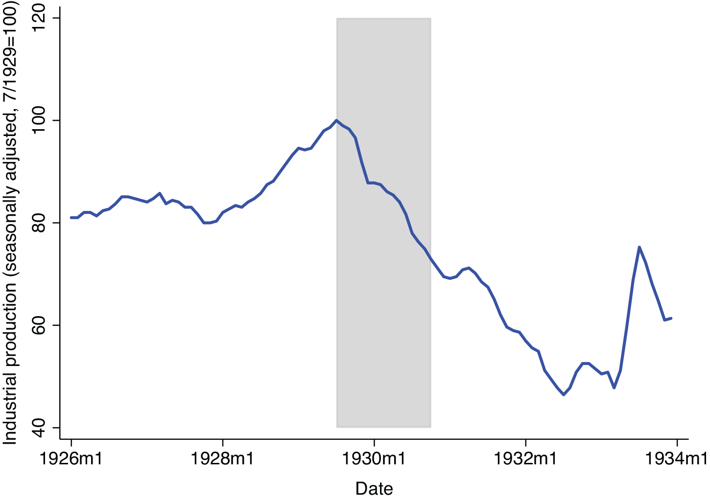
The first year of the Great Depression in the United States was exceptionally severe, much more severe than that in other countries. Figure 1 shows the path of U.S. industrial production in the first year of the Great Depression.Footnote 1 Had the U.S. Depression ended in 1930, the output decline would still have been more severe than that in any other post-1869 recession with the exception of 1945–46.Footnote 2 Industrial production fell 27 percent from its peak in July 1929 to October 1930; year-on-year, in 1930, real GDP fell 8.5 percent.Footnote 3 In her sample of 23 countries, Romer (Reference Romer1993, table 1) finds that the United States was the only country in 1930 to see a year-over-year decline in industrial production of more than 20 percent; among the 15 countries in which industrial production fell, the median decline was 9 percent (Romer Reference Romer1993, p. 21).

Figure 1 INDUSTRIAL PRODUCTION
Note: Shading indicates July 1929 to October 1930, the period of the Great Depression before the first banking panic.
Source: FRED series INDPRO.
Table 1 FARM PRODUCT PRICES

Notes: Prices are producer prices (prices received by farmers); annual prices are unweighted calendar year averages. Farm product value equals physical production times price. Farm product value and production figures are for the crop year, which is not necessarily the calendar year. For further notes, see Online Appendix A.
Source: See Online Appendix A.
We argue that the size and characteristics of the agricultural sector explain part of why initial negative shocks resulted in a large downturn. This helps to account for why 1930 was an exceptionally bad year for the U.S. economy despite the continued stability of the banking system through most of the year. The worldwide recession that began in summer 1929 quickly lowered the prices of farm products, particularly those of internationally traded crops. These price declines in turn depressed farmers’ incomes. Likely because lower farm incomes interacted with fixed nominal debt burdens, spending in agricultural areas collapsed. We estimate that absent this propagation through the agricultural sector, the output decline in the first year of the Depression would have been at least 10 to 30 percent smaller.
To document the importance of farmers for the severity of the early U.S. Great Depression, we proceed in four steps. First, in the next section, we show that at the beginning of the Depression, farm product prices fell rapidly in both absolute and relative terms, depressing farm incomes. These price declines were particularly large for crops exposed to world demand. Entirely because of price declines, the combined dollar value of U.S. cotton, wheat, and tobacco production fell 38 percent between 1929 and 1930.Footnote 4
We then show that in 1930 the spending of farmers fell relative to nonfarmers. To examine farm spending, we use monthly auto sales data by state and newly-collected data on auto sales in Ohio counties.Footnote 5 We find that in the first year of the Depression, spending fell more in states and counties most exposed to falling crop prices. The cross-sectional effect of exposure to farm product price declines was large: a one-standard-deviation increase in the share of a state’s population living on farms was associated with a 5.5 percentage point larger decline in auto sales between the second and third quarter of 1929 and the second and third quarter of 1930. Qualitatively similar results in some (though not all) specifications in the county and state data increase our confidence in the economic significance of the relationship between farming and the Depression. The similarity of the results across Ohio counties and across U.S. states suggests that this relationship is not simply an idiosyncratic artifact of a few states’ performances.
A large cross-sectional effect of exposure to farm product prices need not indicate an important role for farmers in the aggregate. But redistribution away from farmers would have mattered for the aggregate economy if farmers had higher marginal propensities to consume (MPCs) than the companies, business owners, and workers benefiting from lower farm product prices.Footnote 6 We show that this is plausible because farmers entered the Great Depression with high nominal debt burdens, and because there was incomplete pass-through of lower farm product prices to lower consumer prices.
In the final section of the paper, we use the structure of the model in Hausman, Rhode, and Wieland (Reference Hausman, Rhode and Wieland2019) to obtain a quantitative sense of the effect of falling farm product prices on the severity of the early Great Depression. We ask: If relative farm product prices had not declined before October 1930, how much less severe would the first year of the Depression have been? We find that lower farm product prices likely explain at least 10–30 percent of the output decline that occurred before fall 1930. The large range is due to uncertainty about the relative MPC of farmers and nonfarmers, the pass-through of farm product prices to final goods prices, and the aggregate multiplier.
This paper relates to several themes in the economic history and macroeconomics literatures. Most obviously, we contribute to the literature on the beginning of the Great Depression. Friedman and Schwartz (Reference Friedman and Anna1963, pp. 306–7) emphasize tight monetary policy as a cause of the initial output decline in 1930. By contrast, Temin (Reference Temin1976) and Romer (Reference Romer1993) dispute the importance of tight monetary policy for causing the downturn in 1930 and instead emphasize non-monetary shocks. The literature has pointed to the stock market crash (Romer Reference Romer1990) and consumer debt burdens (Olney Reference Olney1999) as non-monetary shocks that may have contributed to the large decline in U.S. output before the first banking crisis. And in a recent paper, Gorton, Laarits, and Muir (Reference Gorton, Toomas and Tyler2019) argue that despite the lack of depositor runs, bank behavior contributed to the output decline in 1930, as banks cut back on loans in favor of safe assets. Since the upper end of our range for the effect of lower farm product prices on 1930 output still leaves two-thirds of that year’s output decline to be explained, our work is consistent with a large role for the shocks and propagation mechanisms identified by prior authors. We add to this prior work by documenting substantial regional heterogeneity in the severity of the early Great Depression and by arguing that lower farm product prices, income, and spending are a plausible propagation mechanism through which exogenous shocks (e.g., the stock market crash) led to a large output decline.
Relative to the literature on the U.S. Great Depression, the literature on the international Great Depression has put more emphasis on agriculture.Footnote 7 Kindleberger (Reference Kindleberger1973) is concerned with how trade in agricultural products helped to transmit economic distress across countries. He devotes a chapter to “The Agricultural Depression,” and he suggests that low farm product prices could have contributed to the Depression. He refers to the “conventional wisdom that price declines are deflationary in so far as they ‘check confidence, provoke bank failures, encourage hoarding and in various ways discourage investment’” (Kindleberger Reference Kindleberger1973, p. 142). Interestingly, however, he doubts the importance of the effect that we emphasize of a higher MPC among farmers translating lower farm product prices into lower aggregate spending (p. 142).
The more recent literature on agriculture and the international Great Depression is small. Most related to our work are Madsen (Reference Madsen2001) and Federico (Reference Federico2005). Madsen (Reference Madsen2001) examines the role of agricultural prices in transmitting the Great Depression across countries. Like us, he emphasizes that farmers probably had a higher MPC than nonfarmers. Using cross-country data, he concludes that falling agricultural prices likely account for a significant portion of the output decline during the Great Depression. Federico (Reference Federico2005) addresses a similar question but comes to a different conclusion. He is interested in whether conditions in agriculture substantially contributed to the severity of the Great Depression. He concludes that they did not. His evidence comes from (1) an analysis of world farm product demand and supply that suggests little overproduction in the 1920s, and (2) a review of the literature in which he finds limited support for the view that problems in agricultural areas were an independent cause of the nationwide banking panics in the U.S. Great Depression. Relative to Madsen (Reference Madsen2001) and Federico (Reference Federico2005), we are focused more narrowly on one country (the United States) and one year (1929/30). This allows us to look at detailed state and county data.
In addition to our findings’ importance for understanding the aggregate U.S. economy at the beginning of the Depression, we also contribute to the literature on regional heterogeneity in the Depression’s severity. We add to the findings in Garrett and Wheelock (Reference Garrett and David C.2006), Rosenbloom and Sundstrom (Reference Rosenbloom1999), and Wallis (Reference Wallis1989) in two ways. First, we quantify the large role of agriculture in explaining variations in state economic performance at the beginning of the Depression. Second, we show that it was internationally traded crop production rather than agricultural activity as a whole that drove differences in state performance.
We also contribute to a growing literature in macroeconomics on redistribution and MPC heterogeneity. Recent work in macroeconomics has stressed the importance of redistribution and MPC heterogeneity for aggregate outcomes.Footnote 8 We show that these forces are also relevant to understanding the Great Depression.
FARM PRICES AND INCOME
Figure 2 plots an index of farm product prices and, for comparison, the producer price index and the CPI. It shows the extraordinary decline of farm product prices in absolute and relative terms after the summer 1929 business cycle peak. The seasonally adjusted index of farm product prices graphed in Figure 2 fell 2 percent between July and December 1929, and then by more than 20 percent between December 1929 and September 1930. Industrial production peaked in July 1929 and fell rapidly after October (Figure 1). Since the most rapid farm product price declines did not begin until January 1930, this timing strongly suggests that lower farm product prices were not an exogenous shock causing the U.S. Depression. Rather, they were a response to the Depression and, we shall argue, a propagation mechanism worsening the Depression.
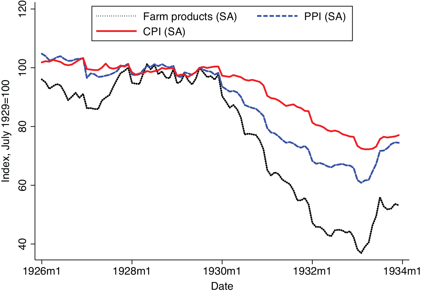
Figure 2 PRICES
Note: The figure shows the level of seasonally adjusted farm product prices, producer prices (PPI), and consumer prices (CPI).
Sources: Farm product prices: FRED series M04058USM350NNBR, originally from NBER series m04058, which was collected from BLS publications; PPI: FRED series PPIACO; CPI: FRED series CPIAUCNS. We seasonally adjust these series using data from 1926 through 1935, excluding 1933 because of the very large farm product price movements in that spring. Seasonally adjusted prices in month t are
 $${e^{{{\hat \varepsilon }_t} + \sum _{j = 1}^{12}{{\hat \beta }_j}/12}}$$
, where
$${e^{{{\hat \varepsilon }_t} + \sum _{j = 1}^{12}{{\hat \beta }_j}/12}}$$
, where
 $${{{\hat \varepsilon }_t}}$$
is the residual from a regression of the price index on monthly dummies, and
$${{{\hat \varepsilon }_t}}$$
is the residual from a regression of the price index on monthly dummies, and
 $${{{\hat \beta }_j}}$$
is the OLS coefficient on the month j dummy.
$${{{\hat \beta }_j}}$$
is the OLS coefficient on the month j dummy.
Why Did Farm Product Prices Fall?
Our focus is on the consequences of the farm product price decline, not its causes. Still, the causes of the farm product price decline are both of independent interest and may matter for the interpretation of our results. The most basic explanation for the price decline is the interaction of a decrease in demand (foreign and domestic) combined with a price inelastic demand curve for farm products and a close to completely price inelastic supply curve. The demand curve for farm products shifted in as the United States and the world fell into recession. For farm products overall, the Depression in the United States certainly played the dominant role; much of farm output was nontraded, and even for traded crops, it mattered that the U.S. output decline in 1930 was more severe than that abroad. The decline in demand had large price effects because in the short term, supply was determined by past planting decisions. And even in the medium term, U.S. farmers facing price declines for their products may have maintained production; a price decline for a farmer has a substitution effect pushing a farmer to plant less but an income effect pushing a farmer to plant more. These forces were combined with an influx of workers into agriculture during the Great Depression, as unemployed urban workers moved to rural areas. Throughout the 1920s, there was net migration from farms/rural areas to cities; this pattern reversed in 1930 with net migration to farms from cities each year from 1930–33 (U.S. Department of Agriculture, 1936, table 445, p. 339). The combination of a growing farm population and an income effect encouraging more production meant that the farm product supply curve was close to vertical during the Depression. As Ezekiel and Bean (Reference Ezekiel and Bean1933, p. 21) put it: “Left to themselves, farmers as a group have been unable to readjust their total production in line with the reduced demands.”Footnote 9 Despite a collapse in wheat prices, for instance, world wheat production rose between the 1929/30 season and the 1931/32 season.Footnote 10
The effect of inelastic supply on the farm product price response was compounded by inelastic demand. Food expenditure is insensitive to price (Taylor and Houthakker Reference Taylor and H. S.2009), likely leading to an inelastic demand curve for farm products primarily used for food. Of course, inelastic supply and demand for farm products were not unique to the Great Depression. Bordo (Reference Bordo1980) notes that at least since Cairnes (Reference Cairnes1873), economists have known that inelastic supply may make commodity prices more volatile than the prices of manufactured goods.Footnote 11 Thus farm product prices often swing dramatically in response to shocks. Beyond these general factors, idiosyncratic shocks drove large price declines of certain farm products. Table 1 shows the prices of 12 major farm products early in the Depression. It illustrates that while the prices of all major farm products fell in 1930, the price decline was far from uniform. It is beyond the scope of the present paper to present a full description and explanation of the behavior of different farm product prices in 1930. Rather we consider one natural distinction, that between more and less internationally traded crops.
In 1930, the prices of wheat, cotton, and tobacco fell more than those of other crops. Cotton, tobacco, and wheat are the three crops in Table 1 that were traded most internationally; Figure 3 illustrates the much larger decline in traded than in nontraded farm product prices after the beginning of the Depression. This distinction was noticed at the time; the U.S. Department of Agriculture (1933, p. 94) wrote “The prices of major cash crops, being more subject to international influence, at first suffered more than did the prices of livestock and livestock products, that are consumed almost entirely in the domestic markets.” To illustrate how international factors mattered, we briefly explore the wheat and cotton price decline.
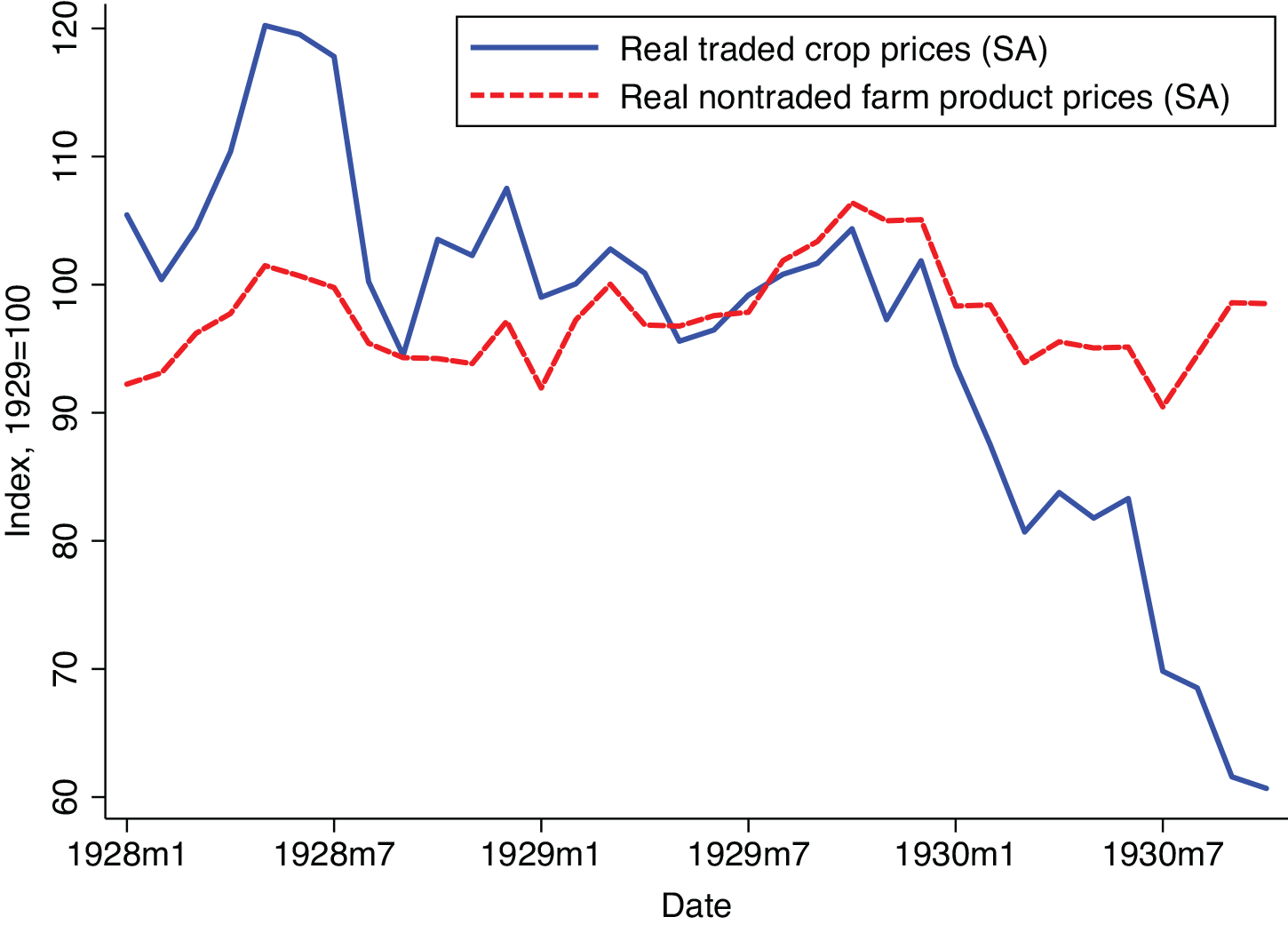
Figure 3 TRADED AND NONTRADED FARM PRODUCT PRICES
Notes: The figure shows seasonally adjusted traded crop and nontraded farm product prices. Traded crops are wheat, cotton, and wool, major internationally traded crops for which monthly price data are available. Tobacco is excluded because only annual prices are available. Nontraded farm products are corn, potatoes, hay, cattle, hogs, milk, eggs, and chickens; these products were traded little internationally. See Online Appendix B for details on the construction of these price indices.
Source: See Online Appendix B.
We start by comparing the price that was received by U.S. wheat and cotton farmers to measures of wheat and cotton prices abroad. Figure 4(a) compares the price of wheat received by U.S. producers to the wholesale price of wheat in Winnipeg, Canada and the wholesale price of imported wheat in Liverpool, England. The figure shows that all three prices followed a roughly similar downward path from fall 1929 to fall 1930. Figure 4(b) compares the price of cotton received by U.S. producers to the prices of U.S. and Indian cotton in Liverpool, England. After the United States, India was the largest exporter of cotton in the late 1920s (U.S. Department of Agriculture 1936, table 112, p. 86). Even more than for wheat, for cotton, there is a close correlation between the U.S. producer price and the two foreign prices. Figures 4(a) and 4(b) suggest, as one might expect with an easily transportable commodity, that world developments determined the prices received by U.S. wheat and cotton farmers. While determining causality is difficult, and quantitatively disentangling the influence of different shocks even more so, it is possible to describe the broad forces lowering world wheat and cotton prices in 1930.
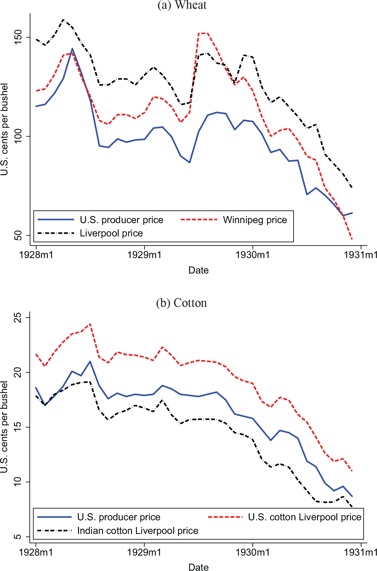
Figure 4 WHEAT AND COTTON PRICES
Notes: All series are non-seasonally adjusted. Figure 4(a) shows wheat prices paid to U.S. producers, the wholesale wheat price of No. 3 Manitoba Northern wheat in Winnipeg, Canada and the price of imported wheat in Liverpool, England. Figure 4(b) shows cotton prices paid to U.S. producers, the wholesale price of American Middling cotton in Liverpool, England, and the wholesale price of Indian Oomra No.1, Fine cotton in Liverpool, England.
Sources: Wheat U.S. Department of Agriculture (1936, table 15, p. 19, table 18, p. 21, and table 19, p. 21). Cotton - U.S. Department of Agriculture (1936, table 106, p. 82 and table 111, p. 85).
World wheat prices fell as the world economy fell into depression, with two more idiosyncratic factors also contributing to the decline. First, world wheat production in 1928/29 was exceptionally large; excluding Russia and China, production rose 9 percent between 1927/28 and 1928/29 (U.S. Department of Agriculture 1936, table 5, p. 11). This led to an accumulation of stocks, which put downward pressure on prices in 1930 ( Wheat Studies, VI:9, Aug. 1930, pp. 387–8; Wheat Studies, VII:2, Dec. 1930, p. 90).Footnote 12
A second idiosyncratic factor pushing down wheat and other grain prices was exports from the Soviet Union. In 1913, before WWI and the Bolshevik revolution, Russia had been the world’s largest wheat producer (U.S. Department of Agriculture 1936, table 5, p. 11). The disruption of WWI and the Russian Civil War reduced Russian wheat production from 1.03 billion bushels in 1913 to a low of 205 million bushels in 1921 (U.S. Department of Agriculture 1936, table 5, p. 11). But production roughly recovered to 1913 levels by 1930 (U.S. Department of Agriculture 1936, table 5, p. 11), and Soviet wheat exports grew from 124,000 bushels in 1928/29, to 7.4 million bushels in 1929/30, and 112 million bushels in 1930/31 (U.S. Department of Agriculture 1933, table 17, p. 417). While it is hard to judge the quantitative significance, we believe it likely that Soviet exports and the prospect thereof depressed wheat prices.
The decline in cotton prices in 1930 is a simpler story. Likely even more for cotton than for wheat, the global depression itself depressed prices. In its summary of the decline in cotton prices during the Depression, the U.S. Department of Agriculture (1933) writes: “The outstanding forces that led to the present cotton situation were general deflation in commodity prices and declines in business activity and consumer incomes throughout the world” (p. 97).Footnote 13 Unlike wheat, which is primarily used to produce food, cotton was used in industry, most obviously, but not only to produce textiles. Thus the demand for cotton was a causality of the world output decline. To give one example of this mechanism, in 1929, the production of car tires accounted for roughly 10 percent of all cotton consumed in the United States (U.S. Department of Agriculture 1933, p. 105). The production of U.S. tire casings fell by 26 percent between 1929 and 1930 with, one imagines, a corresponding hit to demand for cotton.Footnote 14 Of course, world manufacturing output also fell in 1930. As world demand fell, so did the volume of U.S. cotton exports as well as the price. Exports fell from 8.4 million bales in the year beginning August 1928 to 7.0 million bales in the year beginning August 1929. As with wheat, demand for U.S. cotton was also affected by idiosyncratic factors. In particular, manufacturers abroad were increasingly using cheaper foreign, in particular Indian, cotton instead of U.S. cotton (U.S. Department of Agriculture 1931, p. 12).
We draw three conclusions from the wheat and cotton experience. First—and unsurprising—U.S. traded crop prices moved with world prices, meaning that any explanation for the 1930 price decline likely needs to include international shocks. Second, a crop could be tradeable in the sense that its price tracked world prices even if the share of production actually leaving the United States was modest. Exports of wheat in 1930 accounted for less than 20 percent of U.S. wheat production, yet U.S. wheat prices tracked foreign prices closely. Finally, it is difficult to quantify the effect of idiosyncratic versus aggregate shocks and the exact extent to which agricultural price declines were driven by the U.S. Depression and the Depression abroad. This unfortunately means it is difficult to make causal or quantitative statements about the role of foreign versus U.S. shocks in the U.S. farm product price decline. Thus we interpret the results that follow as an exploration of the impact not of an exogenous shock, but rather of a propagation mechanism.
Farm Incomes
The effect of a large commodity price movement depends on its incidence; it was the U.S. economy’s misfortune in 1930 that the burden of lower farm product prices fell on indebted farm households. An individual farmer’s income roughly equals the price of their product times the quantity produced, so the large decline in farm product prices produced a large decline in the income of farmers. Farm incomes are shown in Figure 5. Between July 1929 and October 1930, real, cpi-deflated farm income fell 29 percent; income from crops fell 42 percent. While individuals who became unemployed may have seen larger income declines, the decline in income for the typical farmer was far larger than that for the typical nonfarm worker. Annual nominal income data from the BEA (table SA04) deflated by the CPIFootnote 15 show that real nonfarm personal income fell 6.3 percent between 1929–1930; over the same period, real farm income fell 25.1 percent.

Figure 5 FARM INCOME
Note: The figure shows seasonally adjusted total farm income and income from crop production.
Sources: Pre-1932 – Survey of Current Business, May 1934, p. 19. 1932–33: 1936 Supplement – Survey of Current Business, p. 9. These nominal values are deflated by the CPI (not seasonally adjusted), taken from FRED series CPIAUCNS.
To understand whether the fall in farm income in 1930 was driven by lower farm product prices, Figure 6 shows farm income, the quantity of marketed farm products, and farm product prices from 1927 to 1930. Unlike the series shown in Figure 5, these series are not seasonally adjusted; thus they show the regular seasonal peak in fall of farm products sold and farm income received. Income and marketing track each other closely until mid-1930. This is a bit mysterious given the steady fall in farm product prices. In any case, beginning in mid-1930, farm marketing rises in its typical seasonal fashion while farm income increases little relative to its normal seasonal increase. The unusually small increase in farm income reflects falling farm product prices. The behavior of these series shows that before mid-1930 falling seasonally adjusted farm incomes (Figure 5) may have largely reflected less marketing of farm products. Reduced marketing may in part have been a result of drought, which shrank the 1929 harvest. (In our cross-state regression, we control for drought conditions.) In any case, beginning in summer 1930 lower farm product prices are the likely driver of lower farm incomes.
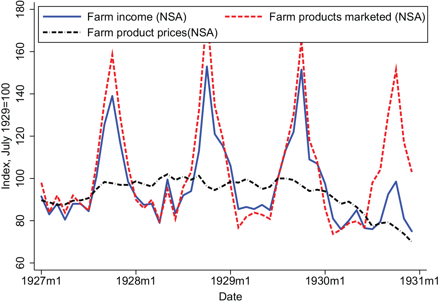
Figure 6 FARM INCOME, MARKETING, AND PRICES
Note: The figure shows nominal farm income, the quantity of farm products marketed, and farm product prices. No series is seasonally adjusted.
Sources: Farm income – Survey of Current Business, May 1934, p. 19. Farm marketing – Survey of Current Business, March 1933, p. 20. Farm product prices – FRED series M04058USM350NNBR, originally from NBER series m04058, which was collected from BLS publications.
EXPENDITURE IN FARM AREAS
The large decline in farm product prices and incomes led to a collapse of spending in farm areas. Initial evidence for this comes from a comparison of rural and small-town retail sales with department and variety store sales. Rural and small-town retail sales are a Department of Commerce index (U.S. Department of Commerce 1934a) that uses data on mail order and chain store sales to measure consumption in small towns (those with a population less than 10,000) and on farms.Footnote 16 Department stores were located in urban areas and thus capture a part of urban consumption. They have the disadvantage, however, of being weighted towards higher-priced goods. The U.S. Department of Commerce (1934b) developed an index of variety store sales in part to correct for this bias. The variety store index has the disadvantage for our purpose, however, of being based on a sample that puts a heavy weight on relatively small cities, those with a population less than 100,000. Still, the Department of Commerce saw this series as at least somewhat representative of consumption in urban areas (U.S. Department of Commerce 1934a).
Figure 7 graphs these series between 1929 and 1933. (The rural and variety store indices begin in January 1929.) The indices start to diverge in December 1929; between July 1929 and October 1930, seasonally adjusted department store and variety store sales fell 7 percent; rural and small-town retail sales fell 28 percent.
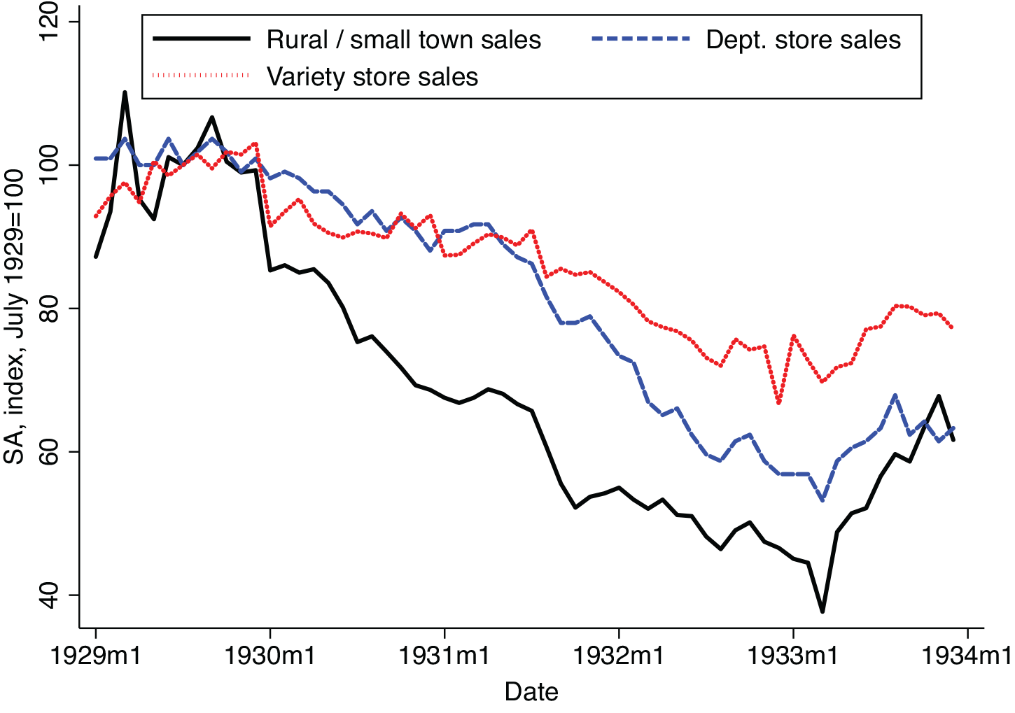
Figure 7 RURAL AND URBAN RETAIL SALES
Note: All series are seasonally adjusted.
Sources: Pre-1932 department store sales – 9/1936 Survey of Current Business, p. 19; Pre-1932 rural sales – 12/1934 Survey of Current Business, p. 20; 1932–1933 department store and rural sales – 1936 Survey of Current Business Supplement, pp. 27–28; variety store sales – 3/1934 Survey of Current Business, p. 18.
While this is already evidence of a large relative decline in consumption in farm areas, we turn to state and county data to more precisely quantify the evolution of spending in farm versus nonfarm areas. In particular, we focus on data on auto sales. Auto sales have three advantages. First, the data are available monthly by state and monthly by county in Ohio. We know of no other indicator of expenditure available by state or county at this frequency. Second, the data are likely to be relatively well-measured, given that car registration was required. Finally, while only one component of household spending, cars played an outsized role in the initial year of the Great Depression. As emphasized by Romer (Reference Romer1990), in 1930 durables consumption fell much more than non-durables consumption.
Evidence from the U.S. States
Monthly data on new passenger car registrations come from the 1934 Automotive Daily News Review and Reference Book.Footnote 17 These data closely approximate sales and for conciseness, we will generally refer to auto “sales” rather than “new registrations.” States required the registration of new cars, so new registrations were a direct measure of sales. As discussed further in Online Appendix C, at times the measure could be inexact, but only to a limited degree.
Figure 8 shows a scatter plot of the percent change in new registrations (sales) between the second and third quarter of 1929 and the second and third quarter of 1930 and the share of a state’s population living on farms. Here and in our regressions later we compare car sales between these six-month averages (1929:Q2–Q3 and 1930:Q2–Q3), since doing so filters out idiosyncratic noise in the monthly data, and since using a 12-month sample window allows us to avoid the uncertainty associated with seasonal adjustment. Figure 8 shows a clear negative relationship between car sales growth and farm share of the population during the first year of the Great Depression.

Figure 8 PERCENT CHANGE IN CAR SALES AND FARM POPULATION SHARE
Sources: Car sales – see text; farm share of the population – Haines and ICPSR (Reference Haines2010).
Figure 9(a) provides another way to see the relationship between farm share and economic performance. It graphs the average level of auto sales in each of four quartiles of states, where states are grouped by the share of their population living on farms. To construct this graph, we seasonally adjust auto sales using data from 1929 (when the series begins) through 1934, excluding 1933.Footnote 18 We note that before 1930 there is no consistent ranking of auto sales by farm quartile, which is to say there is no apparent pre-trend. There is a notable upward spike in auto sales in quartile 4 in late 1929. This upward spike is driven by very high auto sales in Alabama and Mississippi, numbers that we suspect may be errors. For this reason, Figure 9(b) repeats the calculation with Alabama and Mississippi excluded.
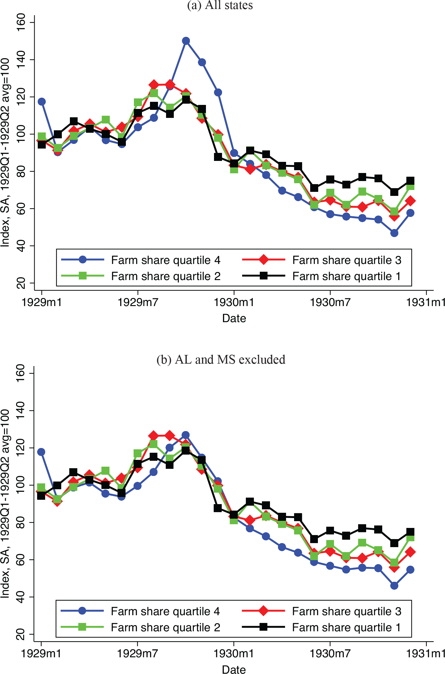
Figure 9 CAR SALES BY FARM SHARE QUARTILE
Sources: Car sales – see text; farm share of the population – Haines and ICPSR (Reference Haines2010).
The first indication of a divergence between high and low farm share quartiles begins in February or March 1930 depending on whether Alabama and Mississippi are included. In these months we first see the expected pattern: the least farm intensive states have the smallest drop in car sales (relative to 1929), followed by quartiles 2 and 3, with the largest decline in car sales occurring in quartile 4. While this timing accords with the drop in farm product prices in Figure 2, one needs to be cautious in reading too much into short-term movements given the uncertainty associated with the seasonal adjustment. Still, by the second half of 1930, a clear pattern emerges, in which auto sales had fallen most in the highest farm share states (quartile 4) and least in the lowest farm share states (quartile 1).
Table 2 investigates the relationship between farm intensity and auto sales more carefully by estimating regressions of the form:
 $$\% \Delta {\rm{Auto}}\;{\rm{sale}}{{\rm{s}}_{i,{\rm{1929}}:{\rm{Q2 - Q3 - 1930}}:{\rm{Q2 - Q3}}}} = {\beta _0} + {\beta _1}{\rm{Agricultural}}\;{\rm{exposur}}{{\rm{e}}_i} + \gamma '{{\rm{X}}_{\rm{i}}}{\rm{ + }}{\varepsilon _{\rm{i}}},$$
where
 $${\rm{\% }}\Delta {\rm{Auto\;sale}}{{\rm{s}}_{i,{\rm{1929:Q2 - Q3 - 1930:Q2 - Q3}}}}$$
is auto sales growth in state i at the beginning of the Depression, “Agricultural exposure” is a measure of a state i’s exposure to falling farm prices, and X is a set of control variables. Column (1) shows results for the single-variable regression analogous to the scatter plot in Figure 8. The coefficient is both economically and statistically significant (the t-statistic equals 5). The coefficient of –0.32 implies that a one-standard-deviation change in farm population share (17 percentage points) is associated with a 5.5 percentage point decline in auto sales growth. For comparison, nationwide auto sales fell 34 percent over this period.Footnote
19
Note also that the R2 is 0.30: as measured by auto sales, the farm share of the population alone explains 30 percent of the cross-state variation in the severity of the early Great Depression.
$${\rm{\% }}\Delta {\rm{Auto\;sale}}{{\rm{s}}_{i,{\rm{1929:Q2 - Q3 - 1930:Q2 - Q3}}}}$$
is auto sales growth in state i at the beginning of the Depression, “Agricultural exposure” is a measure of a state i’s exposure to falling farm prices, and X is a set of control variables. Column (1) shows results for the single-variable regression analogous to the scatter plot in Figure 8. The coefficient is both economically and statistically significant (the t-statistic equals 5). The coefficient of –0.32 implies that a one-standard-deviation change in farm population share (17 percentage points) is associated with a 5.5 percentage point decline in auto sales growth. For comparison, nationwide auto sales fell 34 percent over this period.Footnote
19
Note also that the R2 is 0.30: as measured by auto sales, the farm share of the population alone explains 30 percent of the cross-state variation in the severity of the early Great Depression.
Table 2 CROSS-STATE REGRESSIONS

Notes: The dependent variable is the percent change in non-seasonally adjusted car sales from the 1929:Q2–Q3 average to the 1930:Q2–Q3 average; p.c. means per capita. Robust standard errors in parenthesis. *p < 0.1, **p < 0.05, ***p < 0.01.
Sources: New car sales—see text; population and percent of the population on farms—the 1930 Census as reported in Haines and ICPSR (Reference Haines2010); 1929 value of crops sold per capita—the 1940 Census as reported in Haines, Fishback, and Rhode (Reference Haines, Price and Paul2015); 1928 car sales—Automotive Industries, 23 February 1929, p. 271; we construct the drought dummies using data from the National Climate Data Center. Regional fixed effects are dummy variables for the four census regions: northeast, midwest, south, and west.
In interpreting the results in Table 2, it is worth emphasizing that Specification (1) is not directly measuring the change in purchases of cars by farmers themselves; the difference between the change in car sales in more and less farm intensive states is due not only to the purchasing behavior of farmers but also to the purchasing behavior of segments of the population whose livelihood was linked to that of farmers. When farmers’ spending fell, the owner of the local general store may have also foregone an auto purchase.
Column (2) adds control variables to address omitted variable bias concerns. We control for population to assure that the percent of a state’s population living on farms is not simply proxying for a small versus large state effect;Footnote 20 we control for the per-capita number of cars sold in 1928 to assure that estimates are not biased by greater propensities to purchase cars in some states; and we control for region fixed effects to isolate the effects of farm intensity within regions. These control variables have essentially no effect on the coefficient. Column (3) controls for drought with two dummy variables equal to 1 in states that suffered a moderate drought or worse in the second and third quarters of 1930 and 1929.Footnote 21 With the controls for drought, the coefficient on farm share of the population is again little changed.
Column (4) of Table 2 uses an alternative indicator of a state’s agricultural exposure: the value of crops sold per capita in 1929. The coefficient is again economically and statistically significant (t-statistic equal to 4). The coefficient of –0.12 implies that a one-standard-deviation increase in crops sold per capita in a state ($39.70) results in a 4.8 percentage point larger decline in auto sales in the first year of the Depression. This is very similar to the decline in auto sales associated with a one-standard-deviation change in the farm share of the population. Column (5) adds control variables and region-fixed effects. The coefficient shrinks by one-third, but remains economically and statistically significant. Column (6) adds controls for drought. This results in an increase in the coefficient on crops sold per capita.
The results in Table 2 show that agriculture-intensive states suffered more during the first year of the Great Depression. This is consistent with a story in which lower agricultural prices depressed farm incomes and farm consumption and investment. We would also like to know what sort of farm areas did worst in 1930. If spending declined most in areas growing crops whose prices declined most, this would support our argument that lower farm product prices and income lowered farm area spending. To investigate this, we look at how state performance varied with the type of agricultural product produced.
RESULTS BY CROP
Table 3 shows the relationship between the auto sales growth in the first year of the Depression and the production of two categories of farm products: internationally traded crops and nontraded farm products. In distinguishing between traded and nontraded farm products, our goal is to distinguish between those farm products whose prices were likely to be strongly influenced by world demand (e.g., cotton) from those less influenced by world demand (e.g., milk). Whether it reflects the impact of world demand or not, the division between traded and nontraded roughly captures the division between farm products whose prices collapsed in 1930 and those whose prices fell more modestly (Table 1 and Figure 3 ). We define traded crops to be the value of cotton, tobacco, cereals, and wool production. While not all cereals were traded, their substitutability meant that their prices often moved together (Hausman, Rhode, and Wieland Reference Hausman, Rhode and Wieland2019). Nontraded farm production equals nontraded crop production plus the value of dairy and livestock sold. Nontraded crop production is equal to the value of total crop production minus the value of traded crops. We also include corn in the nontraded crops category. Corn is a cereal, and corn prices may have moved with other cereals prices; but movements in corn prices did not necessarily directly impact farm incomes, because corn was often grown to feed hogs. An increase in the market price of corn had little or no effect on many corn farmers’ incomes since the same farmers were using the corn to feed their hogs.Footnote 22
Table 3 CROSS-STATE REGRESSIONS BY FARM PRODUCT TYPE

Notes: The dependent variable is the percent change in non-seasonally adjusted car sales from the 1929:Q2–Q3 average to the 1930:Q2–Q3 average. Corn is included in nontraded crops because of its use in hog production; p.c. means per capita. Robust standard errors in parenthesis.
*p < 0.1, **p < 0.05, ***p < 0.01.
Sources: Per capita farm product production—the 1940 Census as reported in Haines, Fishback, and Rhode (Reference Haines, Price and Paul2015); all other variables—see Table 2.
The first column of Table 3 shows that traded crop production was much more correlated with auto sales than was nontraded farm product production. The coefficient on traded crop production of –0.15 implies that a one-standard-deviation increase in traded crop production ($39) would have resulted in 5.7 percentage points lower auto sales growth. The coefficient is estimated precisely, with a t-statistic above 4 and a 95 percent confidence interval of [–0.21, –0.08]. Thus we can be confident that there was an economically significant relationship between traded crop production and economic performance.
By contrast, conditional on traded crop production, there is no evidence of a negative association between nontraded farm product production and car sales growth in the first year of the Depression. The conclusion remains the same in Columns (2) and (3) when we add control variables. In sum, the cross-state results show that it was traded crop production rather than agricultural production as a whole that was associated with a more severe beginning of the Depression. This is consistent with the much larger declines in traded crop prices than in the prices of farm products as a whole.
Evidence from Ohio Counties
To obtain further evidence on the relationship between agriculture and the severity of the early Great Depression, we collected data on new car registrations in Ohio counties. To our knowledge, these are the only available county-level data on new car registrations at an annual or higher frequency in 1929/30. The data come from the Bulletin of Business Research prepared by the College of Commerce and Administration of the Ohio State University. The data are monthly and are presented as “Registrations of New Automobile Bills of Sales in Ohio Counties” with the source specified as “Clerks of Courts of Listed Counties.”Footnote 23 Unfortunately, the data do not cover all counties: we have data for 50 of the 88 counties in Ohio. But these counties accounted for most car sales; in 1928, more than 80 percent of all new car sales in Ohio occurred in these 50 counties.Footnote 24
The Bulletin of Business Research presents data on both new passenger car sales and new truck sales. Unfortunately, however, there are too few counties with substantial truck sales to make the truck sales data useful for understanding the early Great Depression. Thus we confine ourselves to an analysis of the new passenger car sales. This has the added advantage of easy comparability with our cross-state results, which are only for passenger cars.
Figure 10 presents a cross-county scatter plot analogous to the cross-state scatter plot in Figure 8. Across Ohio counties, there is no clear relationship between farm population share and new car sales growth. Close inspection of the data, however, reveals that the null result is driven by a few counties, in particular, Gallia, Geauga, and Union. These three counties had large portions of their population living on farms but relatively low values of crop production. As discussed previously, it is crop-producing areas that we expect to have suffered most at the beginning of the Depression, because crop prices fell more than farm product prices as a whole. Figure 11 thus shows a similar scatter plot, but with the value of crops sold per capita rather than the proportion of the population living on farms on the x-axis. As expected, here there is a more obvious negative relationship. This results in part from the shift of Gallia, Geauga, and Union Counties from the far right of the graph to near the middle, reflecting their mid-range crop production despite large farm population shares.

Figure 10 OHIO COUNTIES: PERCENT CHANGE IN NEW CAR SALES AND FARM POPULATION SHARE
Sources: Car sales – see text; farm share of the population – Haines and ICPSR (Reference Haines2010).

Figure 11 OHIO COUNTIES: PERCENT CHANGE IN NEW CAR SALES AND VALUE OF CROPS SOLD PER CAPITA
Sources: Auto sales – see text. Crops sold per capita – Haines, Fishback, and Rhode (Reference Haines, Price and Paul2015).
To more formally investigate the relationship in Ohio between agricultural intensity and performance early in the Depression, we run regressions across counties like those estimated across states in the previous section. Specifically, we estimate
 $$\% \Delta {\rm{Auto}}\;{\rm{sale}}{{\rm{s}}_{j,{\rm{1929}}:{\rm{Q2 - Q3 - 1930}}:{\rm{Q2 - Q3}}}} = {\beta _0} + {\beta _1}{\rm{Agricultural}}\;{\rm{exposur}}{{\rm{e}}_j} + \gamma '{{\rm{X}}_{\rm{j}}}{\rm{ + }}{\varepsilon _{\rm{j}}},$$
where
$$\% \Delta {\rm{Auto}}\;{\rm{sale}}{{\rm{s}}_{j,{\rm{1929}}:{\rm{Q2 - Q3 - 1930}}:{\rm{Q2 - Q3}}}}$$
is new auto sales growth in county j at the beginning of the Depression, “Agricultural exposure” is a measure of exposure to falling farm product prices, and X is a set of control variables.
Columns (1) and (2) of Table 4 show the single variable regressions corresponding to the scatter plots in Figures 10 and 11. Columns (3) and (4) add controls for population and 1928 car sales per capita. Unsurprisingly given the scatter plot (Figure 10 ), with and without controls the coefficient on farm share is small and insignificant. By contrast, with and without controls, the coefficient on crop sales per capita is economically and statistically significant. Its magnitude (–0.13) is somewhat larger than that in the cross-state regression with these controls (Column (5) of Table 2). Thus the results support the cross-state finding of an economically significant relationship between the importance of crops in a county and the depth of the Depression in 1929/30. Columns (5) and (6) explore the relationship between traded and nontraded farm product production and auto sales. As in the cross-state results in Table 3, across Ohio counties, the negative impacts of agriculture are driven by the cultivation of traded crops. But the conclusion is more tentative in the Ohio county data than it is in the state data, since when controls are added (Column (6)) the coefficient on traded crops loses statistical significance.
Table 4 CROSS-COUNTY REGRESSIONS

Notes: The dependent variable is the percent change in non-seasonally adjusted new car sales from the 1929:Q2–Q3 average to the 1930:Q2–Q3 average; p.c. means per capita. While we observe monthly new sales in 1929/30 in 50 counties, there are only 49 observations since 1928 sales were not reported for Morgan County. Robust standard errors in parenthesis. *p < 0.1, **p < 0.05, ***p < 0.01.
Sources: New car sales—see text; population and percent of the population on farms—the 1930 Census as reported in Haines and ICPSR (Reference Haines2010); 1929 value of crops sold per capita and farm product categories—the 1940 Census as reported in Haines, Fishback, and Rhode (Reference Haines, Price and Paul2015); 1928 car sales—calculated from the Industrial and Commercial Ohio Yearbook (1930, table XVI, p. 104), which lists by county both 1929 new car sales and the 1928/29 percent change in new car sales.
Unlike the state results, which change little when weighted by population (Online Appendix Table E.1), some of the cross-county specifications are sensitive to population weighting. Specifically, Online Appendix Table E.2 shows that the univariate results (Specifications (1) and (2)) become stronger, with more evidence of a negative relationship between auto sales and farm share or crops sold per capita. But the results with controls (Specifications (3) and (4)) become weaker. When weighted, there is no longer a negative coefficient on crops sold per capita. Reassuringly, weighting strengthens the finding in Columns (5) and (6) that traded crop production drove worse economic performance while nontraded farm product production did not.
Taken together, the cross-county data are supportive of the findings from the cross-state data. The county sample is too small and noisy for precise, statistically significant conclusions in all specifications, but the results support the robust message from the cross-state data that areas producing traded crops suffered most in the first year of the Depression.
Narrative Evidence
Further evidence for the effect of lower farm product prices on car sales comes from narrative evidence. Narrative evidence itself does not establish the importance of a channel from farm product prices to car sales. But combined with the previous quantitative evidence, it is reassuring. That contemporaries noticed the channel from farm product prices to auto sales suggests that the effect was significant; it supports the mechanism we posit, in which lower farm product prices reduced farmers’ incomes and hence their expenditure.
Narrative evidence comes from the publication Automobile Topics, which reported on car sales conditions around the country. In the summer and fall of 1930, it reports many instances of lower farm product prices depressing sales. The 2 August 1930 edition includes these reports:
-
“IOWA - Grain prices are too low. Farmers will not buy” (p. 1028).
-
“MICHIGAN - Better prices for agricultural products would help sales” (p. 1028).
-
“SOUTH DAKOTA - Prices of farm products hurting our business” (p. 1028).
Similar comments were made in the 4 October 1930 issue:
-
“SOUTH CAROLINA - Prices on cotton and tobacco retarding sales” (p. 678).
-
“GEORGIA - Low price of cotton hurting” (p. 678).
-
“NORTH DAKOTA - Poor crops and low grain prices retarding sales. There can be no prosperity here until grain prices go up” (p. 678).
To be sure—and consistent with our argument—low farm product prices are far from the only factor discussed in Automobile Topics. Many quotes are also to be found on depressed conditions in manufacturing, on complaints about banks, and on idiosyncratic local conditions. Like our quantitative evidence, however, the narrative evidence is consistent with a large role for lower farm product prices in explaining lower auto sales in 1930.
REDISTRIBUTION
Lower farm product prices transferred income from the farm sector to the rest of the economy, and we have shown that spending fell in farm relative to nonfarm areas. This does not establish, however, that lower farm product prices harmed the economy as a whole. Like Madsen (Reference Madsen2001), we believe that a mechanism through which the transfer of income away from farmers was on net contractionary is that farmers likely had a higher MPC than the agents benefiting from lower farm product prices.
Unlike the econometric evidence of the previous section, the evidence for a relatively high MPC among farmers is fragmentary. The first piece of evidence is farmers’ debt burden. As the quote from Irving Fisher that begins this paper suggests, low farm product prices and incomes posed particularly severe problems for farmers because of large nominal debt burdens. In 1930, farm mortgage debt was 190 percent of net farm personal income.Footnote 25 By contrast, residential mortgage debt was 39 percent of nonfarm personal income.Footnote 26 High farm debt burdens were reflected in large numbers of farm foreclosures. In 1929 and 1930, there were 14.7 and 15.7 foreclosures per 1,000 farms. This indicates a severe level of distress relative to other times; during the boom period of 1913–20, foreclosures per 1,000 farms averaged 3.2 and even between 1921 and 1925—after farm product prices fell in the aftermath of WWI—foreclosures per 1,000 farms averaged 10.7, roughly 50 percent less than in 1929/30 (Alston Reference Alston1983, table 1, p. 888).
These debt problems were long in the making. Farmers acquired debt during WWI as farm product prices and farmland values rose. Nominal debt continued to rise in the 1920s even as farm product and farmland prices fell (Wickens Reference Wickens1932; Alston Reference Alston1983). This put farmers in a perilous position on the eve of the Great Depression: when farm product prices fell in 1929/30, real farm debt burdens rose to very high levels. Table 5 shows that the ratio of farm debt to gross income and the ratio of farm debt to assets roughly doubled between 1910 and 1930. The debt to gross income ratio increased by 20 percent just between 1928 and 1930.
Table 5 FARM DEBT

Notes: Debt is farm mortgage debt. Assets are the value of farmland and buildings.
Source: Clark (Reference Clark1933, table 5, p. 28).
One would expect these large nominal debt burdens to have increased the difficulties farmers faced from lower farm product prices in 1930. As farmers’ incomes fell, debt service absorbed more of their income, squeezing their spending. Olney (Reference Olney1999) argues that a similar mechanism affected households burdened by consumer debt, contributing to the economy-wide collapse of spending in 1930. To understand the contribution of farm mortgage debt to the collapse of spending in farm states, we start by examining the univariate relationship between auto sales over our sample period (1929:Q2–Q3 to 1930:Q2–Q3) and farm leverage in a state, with leverage defined as assets/(assets–debt), where debt is equal to farm mortgage debt, and assets are equal to the value of farm land and buildings.
Figure 12 shows a scatter plot of this relationship. There is some evidence of a negative relationship, though it is not statistically significant when Washington, D.C. (an obvious outlier with little agriculture) is excluded. Of more interest than this bivariate relationship would be whether the interaction of traded crop production and farm leverage was a determinant of auto sales in 1930. (We focus on traded crops because those are the farm products whose prices fell most.) The hypothesis—consistent with Olney (Reference Olney1999)—is that the negative effect of traded crop production on auto sales would have been largest in those areas with the most farm leverage. In other words, we expect farmers to have cut back most on spending in response to farm product price declines in places where their debt burdens were heaviest.

Figure 12 PERCENT CHANGE IN CAR SALES AND FARM LEVERAGE
Sources: Car sales – see text; farm leverage – authors’ calculations (see text) from data on debt and assets in Haines, Fishback, and Rhode (Reference Haines, Price and Paul2015).
To test this hypothesis, we would like to estimate:
 $$\% \Delta {\rm{Auto}}\;{\rm{sale}}{{\rm{s}}_{i,{\rm{1929}}:{\rm{Q2 - Q3 - 1930}}:{\rm{Q2 - Q3}}}} = {\beta _0} + {\beta _1}{\rm{Traded}}\;{\rm{crop}}\;{\rm{p}}.{\rm{c}}{._i} + {\beta _2}{\rm{Leverag}}{{\rm{e}}_i} + {\beta _3}{\rm{Traded}}\;{\rm{crop}}\;{\rm{p}}.{\rm{c}}{._i} \times {\rm{Leverag}}{{\rm{e}}_i} + \gamma '{{\rm{X}}_{\rm{i}}}{\rm{ + }}{\varepsilon _{\rm{i}}}.$$
The problem is that with 49 observations we lack the statistical power to do this estimation; in our 49 observation sample, there is essentially no variation in the interaction term that is not explained by the level of traded crop production and leverage. The R 2 of the regression of the interaction on the levels of traded crop production and leverage is 0.998. Thus we cannot plausibly identify
 $${\beta _3}$$
.
$${\beta _3}$$
.
Despite our inability to estimate Equation (3), we have three reasons to believe that
$${\beta _3}$$
is negative, that more debt was associated with a larger decline in spending when farm product prices fell. First, a negative
$${\beta _3}$$
is predicted by theory. One way to see this is to note that a debt burden is likely to indicate one or more of the following: (1) that an agent expects income to be higher in the future; (2) that an agent is an impatient, hand-to-mouth consumer; or (3) that an agent is liquidity constrained. (1) would be the case, for instance, if a farmer borrowed with the expectation that farm product prices would be higher in the future; (2) would occur if a farmer wished to consume as much as possible in the present; (3) would occur if a farmer wanted to finance a large purchase, for example, of more land, without sufficient cash on hand to make the purchase. All these possibilities suggest that the presence of debt will coincide with a lack of savings and thus that the response to an income decline will be a large decline in consumption.
In addition to this economic logic, limited empirical evidence is consistent with a correlation between debt and a higher MPC. In Hausman, Rhode, and Wieland (Reference Hausman, Rhode and Wieland2019), we estimate a regression similar to Equation (3) on nationwide county auto sales data in 1933, when farm product prices rose; we find that higher farm product prices had a larger effect on spending in counties where more farms were mortgaged. More recent evidence from the 2008 financial crisis is also consistent with a correlation between higher debt burdens and a higher MPC; Mian, Rao, and Sufi (Reference Mian, Kamalesh and Amir2013) find that in 2008 more leverage was associated with a higher MPC.
The second argument suggesting that farmers had a relatively high MPC concerns the distribution of the benefits of lower farm product prices. Insofar as lower farm product prices benefited urban workers, many of whom were losing their jobs in 1930, it is not obvious that the difference between the MPCs of the winners and losers would be large. Limited pass-through meant, however, that it was businesses as well as workers who benefited from lower farm product prices. And it is quite plausible that the marginal propensity to spend of businesses was much below that of farmers.Footnote 27
Limited pass-through was driven by the stickiness of many final goods prices at the beginning of the Depression. For example, while the producer price of tobacco fell 23 percent from 1929–1930, the price of a pack of cigarettes rose 2 percent.Footnote 28 Retail bread prices fell 0.17 cents per pound while the price of the farm product input fell 0.26 cents.Footnote 29 And while the price of the wheat input to a 28-oz package of wheat cereal fell by 0.8 cents between 1929:Q2–Q3 and 1930:Q2–Q3, the retail price fell only 0.2 cents (U.S. Department of Agriculture 1945, table 42, p. 195). These (and other) examples suggest that in 1930 businesses producing final goods from farm products often benefited from lower farm product prices.Footnote 30
AGGREGATE EFFECT
To obtain a quantitative sense of how farmers’ relatively high MPC could have led to aggregate effects of lower farm product prices, we follow Hausman, Rhode, and Wieland (Reference Hausman, Rhode and Wieland2019). In that framework, output is demand-determined (prices are sticky) so changes in aggregate consumption and investment demand resulting from lower farm product prices affect output. In Hausman, Rhode, and Wieland (Reference Hausman, Rhode and Wieland2019), we argue that the aggregate effect of a farm product price change on car sales can be approximated by
 $$\% {\rm{ }}\Delta cars = \underbrace {\beta \times {\phi ^f}}_{\scriptstyle naive \atop
\scriptstyle {\rm{extrapolation}} } \times \underbrace {{{{\rm{Farm area income per capita}}} \over {{\rm{Nationalincomeper capita}}}}}_{{\rm{Relative income p}}{\rm{.c}}{\rm{.}}} \times \underbrace {\left( {1 - \xi {{{\theta ^w}} \over {{\theta ^f}}}} \right)}_{\scriptstyle {\rm{Redistribution from}} \atop
\scriptstyle {\rm{ high - MPC consumers}} } \times \underbrace {{\mu _t}}_{\scriptstyle {\rm{Aggregate}} \atop
{\scriptstyle {\rm{spending}} \atop
\scriptstyle {\rm{multiplier}} }} + \underbrace { - \sigma d\ln (1 + {r_t})}_{{\rm{Intertemporal Substitution}}}.$$
$$\% {\rm{ }}\Delta cars = \underbrace {\beta \times {\phi ^f}}_{\scriptstyle naive \atop
\scriptstyle {\rm{extrapolation}} } \times \underbrace {{{{\rm{Farm area income per capita}}} \over {{\rm{Nationalincomeper capita}}}}}_{{\rm{Relative income p}}{\rm{.c}}{\rm{.}}} \times \underbrace {\left( {1 - \xi {{{\theta ^w}} \over {{\theta ^f}}}} \right)}_{\scriptstyle {\rm{Redistribution from}} \atop
\scriptstyle {\rm{ high - MPC consumers}} } \times \underbrace {{\mu _t}}_{\scriptstyle {\rm{Aggregate}} \atop
{\scriptstyle {\rm{spending}} \atop
\scriptstyle {\rm{multiplier}} }} + \underbrace { - \sigma d\ln (1 + {r_t})}_{{\rm{Intertemporal Substitution}}}.$$
 $$\beta $$
is the coefficient from the cross-state regression of the percent change in car sales on the farm share of the population. From Column (1) of Table 2, this is –0.32.
$$\beta $$
is the coefficient from the cross-state regression of the percent change in car sales on the farm share of the population. From Column (1) of Table 2, this is –0.32.
 $${\phi ^f}$$
is the farm share of the U.S. population, which in 1930 was 24.8 percent. We call the product of
$$\beta $$
and
$${\phi ^f}$$
a naive extrapolation since it is what one would guess about the aggregate effect from assuming that the aggregate effect of farmers on economic performance was exactly equal to the cross-sectional effect.
$${\phi ^f}$$
is the farm share of the U.S. population, which in 1930 was 24.8 percent. We call the product of
$$\beta $$
and
$${\phi ^f}$$
a naive extrapolation since it is what one would guess about the aggregate effect from assuming that the aggregate effect of farmers on economic performance was exactly equal to the cross-sectional effect.
As discussed earlier, this naive extrapolation is wrong since the cross-sectional coefficient measures both the negative effect of lower farm product prices on farmers and the positive effect of lower farm product prices on nonfarmers. We assume that there are two types of nonfarmers: capitalists and workers. By assumption, capitalists have a MPC of zero, so that gains from lower farm product prices absorbed by businesses have no effect on aggregate demand. Thus, for instance, we assume that the gains of cigarette manufacturers from lower tobacco prices do not lead to more investment spending by cigarette manufacturers. Nonfarm workers, by contrast, do have a positive MPC, and we assume that they spend a substantial fraction of their gains from lower farm product prices. We believe this assumption to be reasonable given, for instance, the evidence in Gelman et al. (Reference Gelman, Yuriy, Shachar, Dmitri, Matthew, Dan and Steven2019) on consumers’ spending response to lower gas prices in 2014–2015; Gelman et al. (Reference Gelman, Yuriy, Shachar, Dmitri, Matthew, Dan and Steven2019) find an MPC near 1 from the increase in income due to lower gas prices. While gas prices may be uniquely salient, it is likely that lower farm product prices, insofar as they passed through to lower consumer (e.g., food) prices, did increase real worker spending, including that on cars.
These assumptions are reflected in our adjustment for redistribution.Footnote
31
The adjustment factor,
 $$\xi \frac{{{\theta ^w}}}{{{\theta ^f}}}$$
, equals the extent to which lower farm product prices were passed through to workers (
$$\xi \frac{{{\theta ^w}}}{{{\theta ^f}}}$$
, equals the extent to which lower farm product prices were passed through to workers (
 $$\xi $$
) times the ratio of the MPC of workers (
$$\xi $$
) times the ratio of the MPC of workers (
 $${\theta ^w}$$
) to the MPC of farmers (
$${\theta ^w}$$
) to the MPC of farmers (
 $${\theta ^f}$$
). As in Hausman, Rhode, and Wieland (Reference Hausman, Rhode and Wieland2019), we consider a range of values for the redistribution factor,
$${\theta ^f}$$
). As in Hausman, Rhode, and Wieland (Reference Hausman, Rhode and Wieland2019), we consider a range of values for the redistribution factor,
 $$\xi \frac{{{\theta ^w}}}{{{\theta ^f}}}$$
, of 0.3 to 0.7, and a range for the aggregate spending multiplier of 1 to 3. Also as in Hausman, Rhode, and Wieland (Reference Hausman, Rhode and Wieland2019), we ignore the possible quantitative contribution of intertemporal substitution, in other words, the contractionary effect of lower inflation expectations caused by lower farm product prices.
$$\xi \frac{{{\theta ^w}}}{{{\theta ^f}}}$$
, of 0.3 to 0.7, and a range for the aggregate spending multiplier of 1 to 3. Also as in Hausman, Rhode, and Wieland (Reference Hausman, Rhode and Wieland2019), we ignore the possible quantitative contribution of intertemporal substitution, in other words, the contractionary effect of lower inflation expectations caused by lower farm product prices.
The results of this exercise are shown in Table 6. Columns (1) through (3) show the percent decline in car sales accounted for by lower farm product prices for given assumptions about the redistribution factor and the aggregate multiplier. Columns (4) through (6) divide these estimates by the total decline in new car sales growth from 1929:Q2–Q3 to 1930:Q2–Q3 to show the fraction of the decline in new car sales growth explained by lower farm product prices. These estimates show that lower farm product prices had a significant effect on auto sales in the initial year of the Depression unless one believes: (1) that lower farm product prices were passed through to urban workers (
$$\xi $$
high), (2) that urban workers had a MPC similar to farmers (
$${\theta ^w}$$
close to
$${\theta ^f}$$
), and (3) that the aggregate multiplier was low. For example, a mid-range estimate of the redistribution factor (0.5) and of the aggregate multiplier (2) suggests that had farm product prices not fallen, the decline in auto sales would have been 15 percent smaller.
Table 6 IMPLIED AGGREGATE EFFECT

Notes: Columns (1)–(3) display the implied new car sales growth rate from Equation (4) given the indicated parameter values, and
 $$\beta = - 0.32$$
,
$$\beta = - 0.32$$
,
 $${\phi ^f} = 0.248$$
, and
$${\phi ^f} = 0.248$$
, and
 $$\frac{{{Y_{p.c.,a}}}}{{{Y_{p.c.}}}} = 0.66$$
;
$$\frac{{{Y_{p.c.,a}}}}{{{Y_{p.c.}}}} = 0.66$$
;
 $$\frac{{{Y_{p.c.,a}}}}{{{Y_{p.c.}}}}$$
is the ratio of 1929 per capita income in states with farm population greater than the national average in 1930 to per capita income in all states. Columns (4)–(6) show the fraction of actual new car sales growth explained. Actual new car sales growth in our sample period, 1929:Q2–Q3 to 1930:Q2–Q3, was –34 percent (NBER macrohistory series m01109).
$$\frac{{{Y_{p.c.,a}}}}{{{Y_{p.c.}}}}$$
is the ratio of 1929 per capita income in states with farm population greater than the national average in 1930 to per capita income in all states. Columns (4)–(6) show the fraction of actual new car sales growth explained. Actual new car sales growth in our sample period, 1929:Q2–Q3 to 1930:Q2–Q3, was –34 percent (NBER macrohistory series m01109).
Sources: Income data are from BEA table SA4 and population data are from Haines and ICPSR (Reference Haines2010).
So far we have discussed the impact of lower farm product prices on auto sales. We are ultimately interested in the effect on aggregate output. Fortunately, one can reasonably assume that the share of the auto sales decline explained by lower farm product prices is roughly equal to the share of the output decline explained by lower farm product prices.Footnote
32
If one considers the ratio shown in Columns (4) to (6):
 $$\frac{{{\rm{impact\;on\;car\;sales\;growth}}}}{{{\rm{actual\;car\;sales\;growth}}}}$$
, both the numerator and denominator are likely larger than they would be for a measure of output. The numerator is likely larger since it is plausible that farmers cut back more on auto purchases than on purchases of other items, for example, nondurable goods. And we know from data that the denominator is larger: over our sample period, between the second and third quarter of 1929 and the second and third quarter of 1930, new car sales declined 34 percent while industrial production declined 23 percent (NBER macrohistory series m01109 and FRED series INDPRO). Thus—while obviously subject to uncertainty—we take the estimates in Columns (4) to (6) to be reasonable estimates of the share of the 1929–30 output decline explained by lower farm product prices.
$$\frac{{{\rm{impact\;on\;car\;sales\;growth}}}}{{{\rm{actual\;car\;sales\;growth}}}}$$
, both the numerator and denominator are likely larger than they would be for a measure of output. The numerator is likely larger since it is plausible that farmers cut back more on auto purchases than on purchases of other items, for example, nondurable goods. And we know from data that the denominator is larger: over our sample period, between the second and third quarter of 1929 and the second and third quarter of 1930, new car sales declined 34 percent while industrial production declined 23 percent (NBER macrohistory series m01109 and FRED series INDPRO). Thus—while obviously subject to uncertainty—we take the estimates in Columns (4) to (6) to be reasonable estimates of the share of the 1929–30 output decline explained by lower farm product prices.
Importantly, this may be a conservative, lower bound for the impact of lower farm product prices on the U.S. economy. Because of the difficulty in quantifying the effect, in our calculation, we deliberately exclude the contractionary effect of lower farm product prices operating through deflation and deflationary expectations. But this effect could have been large: plummeting farm product prices were one of the early indicators of the severe deflation that began in 1930.
CONCLUSION
We argue that the agriculture sector played an important role in propagating negative shocks that hit the U.S. economy in 1929 and 1930. Declines in world demand translated into large declines in farm product prices and farmers’ incomes. Income declines in turn lowered farmers’ expenditure, a process likely intensified by farmers’ large nominal debt burdens.
We find that between mid-1929 and mid-1930 car sales fell most in states most exposed to farm product price declines. While less robust, we find a similar pattern across Ohio counties. The rough consistency of the county results with the state results is reassuring evidence that the effect we find is real and is not an artifact of a spurious cross-state correlation. The cross-sectional results are themselves of interest; they show, for instance, that knowing the farm share of a state’s population in 1930 is quite predictive of the severity of a state’s economic contraction in 1930. We are, however, ultimately interested in the aggregate implications of low farm product prices. To estimate these, we used a model, and our calculations were necessarily more speculative. But a plausible range of parameters suggests that the mechanism through which farm product prices lowered spending by farmers explains 10–30 percent of the decline in U.S. output before the first banking crisis.
Our results point to limits put on policy by the gold standard. Had the United States left the gold standard and devalued the dollar in 1930, it could have avoided much of the decline in farm product prices. Leaving the gold standard in 1930 would have increased dollar-denominated farm product prices just as it did in 1933 (Hausman, Rhode, and Wieland Reference Hausman, Rhode and Wieland2019); 30 percent lower wheat prices in Liverpool and a 30 percent weaker dollar would have meant unchanged wheat prices for U.S. farmers. Of course, lower farm product prices were just one consequence of U.S. adherence to the gold standard; more important were the real or perceived limits on monetary policy imposed by the gold standard later in the Depression (Eichengreen Reference Eichengreen1992).
This paper’s concern is with a specific historical episode. But there are contemporary implications. A growing theoretical and empirical literature in macroeconomics shows the importance of redistribution as a propagation mechanism for macroeconomic shocks. Much of the empirical motivation for this literature comes from the experience of the 2008–2009 financial crisis and recession in which the costs of falling house prices were concentrated on indebted households. The large spending response of these households to this negative shock was a key driver of the recessions’ severity (Mian, Rao, and Sufi Reference Mian, Kamalesh and Amir2013).
Farmers in 1930 are the analog to mortgaged households in 2008. They had high levels of debt and their spending was sensitive to income declines. Just as declines in spending by mortgaged households explain a part of the 2008–2009 recession, so declines in farmers’ spending explain part of the early U.S. Great Depression. This result supports macroeconomists’ recent focus on redistribution. It is also a reminder of the value of a detailed understanding of an economy’s structure even for aggregate questions. Redistribution effects depend on the distribution of income and the spending propensities of the affected groups. Thus our work also supports the long-standing concern of economic historians with agriculture in the interwar period.