
The fact of Malden being a “no-license” city has been the cause of many people choosing it as a place of residence […] The result of the absence of the sale of liquor is that we have the cleanest of streets, a large absence of crime, many who own their own homes, a savings bank with large deposits, and everything that goes to make us a happy and prosperous community.
—George Louis Richards, Mayor of Malden, Massachusetts 1908 Anti-Saloon League HandbookProhibition, a set of laws to restrict alcoholic beverages, was a major policy issue at the beginning of the twentieth century. Efforts to limit access to alcohol culminated with the ratification of the Eighteenth Amendment and the passage of the Volstead Act in 1919, which made the production and sale of alcoholic beverages illegal nationwide. Prohibition, however, did not originate as a federal policy: in 1919, the country was already a patchwork of dry laws at the state, county, and local levels. As the quote from Richards illustrates, local Prohibition aimed to rid communities of not only alcohol consumption but also its negative consequences. For the mostly rural areas that enacted it, Prohibition was a major local policy change.
In this paper, we investigate the local equilibrium effects of this policy. Prohibition was a sudden policy change with significant heterogeneity in terms of both preferences and local enactment, making it a good setting to study Tiebout (Reference Tiebout1956) sorting. In addition, Prohibition was a policy that affected the amenity value of a location.Footnote 1 Economists have significant interest in how amenities affect economic activity (e.g., Florida Reference Florida2003; Diamond Reference Diamond2016), but their equilibrium effect can be challenging to identify because most policies that affect amenity values are gradual or extremely local in nature.Footnote 2 Dry laws, being an abrupt policy shock affecting the entire locality, provide a rare opportunity to explore the role of such policy changes in a local economy.
Our empirical strategy estimates the effect of Prohibition by comparing same-state rural counties with similar preferences towards alcohol that introduced dry laws slightly earlier (1900-1909) or slightly later (1910— 1919) in a differences-in-differences design.Footnote 3 The identification assumption is that early and late adopters of local prohibition are on parallel trends. We provide supportive evidence for this assumption using event study specifications.Footnote 4
We find that local Prohibition had significant economic effects on rural counties. First, Prohibition increased population and land prices, consistent with it being a policy that people find desirable. Second, we show that counties that enacted Prohibition saw increases in labor productivity and capital investment after they became dry, consistent with agglomeration that comes through a land price channel. We also see an increase in banks in the areas, suggestive of more lending.Footnote 5 Third, we show counterintuitive sorting patterns: counties with local Prohibition attracted relatively more immigrants and African-Americans. Given that these groups were generally less in favor of Prohibition, these sorting patterns seem unlikely to have been driven by preferences for the policy but could have been the product of growing labor market opportunities.
The causal effect of Prohibition on productivity is one of our more novel results, especially considering that it was not one of the stated goals of the policy. The causal channel we propose is similar to the effect of land prices on investment in modern times (Chaney, Sraer, and Thesmar Reference Chaney, Sraer and Thesmar2012; Bahaj, Foulis, and Pinter Reference Bahaj, Angus and Gabor2020): landowners become wealthier and have more access to collateral, so they can invest more in their businesses or, in this case, farms.Footnote 6 While we do not claim to prove that this channel is the primary channel or the only mechanism through which Prohibition affected productivity, we present several pieces of evidence consistent with it. For example, we see this in a large increase in farm equipment. In addition, looking at heterogeneity across ex ante measures of banking intensity, the effects are stronger in areas with more banks per capita and higher mortgage shares. This result has interesting implications for other policies and suggests that policies improving local amenities could have productivity effects by increasing the value of land.Footnote 7
Prohibition has one major advantage for studying Tiebout (Reference Tiebout1956) sorting and the effects of local policies that affect amenities: it was a large sudden change that affected the amenity value of entire labor markets allowing for difference-in-differences estimation. But it also has a couple of downsides that we work to address. The first disadvantage is that it is not randomly assigned, so plausible identification is a challenge. Because of the historical and political context, we use within-state variation and dynamically control for both baseline preferences towards alcohol and the initial demographic characteristics that predict Prohibition adoption. We think that the remaining variation, possibly due to the timing and scarce resources of the Prohibition movement, can plausibly identify the effects of Prohibition.
The second disadvantage to our setting is that Prohibition could have had direct effects on productivity by making workers more sober.Footnote 8 This seems less likely than our land price channel for a few reasons. First, we find stronger effects in counties with railroads and counties that bordered wet counties. This makes sense because population and land prices would increase more in areas that are more accessible to migrants. It is inconsistent with a sobriety story because alcohol would likely be more accessible in these areas as well. Second, the share of workers in farms decreased. If the productivity increase were due only to more sober workers, we would expect farmers to hire more labor. But if the productivity increase is because of labor-substituting farm equipment, the decrease in farm- employment shares makes sense. Last, while Prohibition did shut down saloons, historians debate to what extent consumption decreased. Counties that passed Prohibition had large numbers of Protestants, many of which would have taken teetotaler pledges with their church (Okrent Reference Okrent2010). And, for those that did drink, they were not prohibited from buying it in a neighboring county or state until the Webb-Simpson Act of 1913.Footnote 9
Our work is directly related to the literature on the effects of alcohol prohibition in the United States and abroad. Previous work has focused on the effect of Prohibition on alcohol consumption (Miron and Zwiebel Reference Miron1991; Dills and Miron Reference Dills2004; Law and Marks Reference Law2020), infant mortality (Jacks, Pendakur, and Shigeoka Reference Jacks, Krishna and Hitoshi2017), violence (Owens Reference Owens2014), crime (Owens Reference Owens2011; Heaton Reference Heaton2012), the brewing industry (Hernández Reference Hernández2016), crop production (Edwards and Howe Reference Edwards and Travis2015), and innovation (Andrews Reference Andrews2020). We add to this by demonstrating that Prohibition had large equilibrium outcomes because it was valued as an amenity. There is renewed interest in this question because of recent changes to laws on marijuana (Caulkins, Kilmer, and Kleiman Reference Caulkins, Beau and Kleiman2016). Indeed, Cheng, Mayer, and Mayer (Reference Cheng, Mayer and Mayer2018) claim the legality of marijuana is a positive amenity that causes house price increases of about 6 percent, and Zambiasi and Stillman (Reference Zambiasi and Steven2020) argue that it increased the population of Colorado by 3.2 percent.Footnote 10
Unlike some of the other papers looking at the effects of Prohibition, we focus only on the pre-Eighteenth-Amendment period, when dry laws were voluntarily introduced by many localities. While the introduction and repeal of Federal Prohibition have desirable qualities for exogeneity, the former was forced upon areas that likely did not value it, and the latter was after it had generally been recognized to have negative social consequences (García-Jimeno Reference García-Jimeno2016). Therefore, only our time period is appropriate for studying the effect of Prohibition as a local policy increasing amenity values.
Our work is related to the literature on the sorting of people into regions with different policies, which began with Tiebout (Reference Tiebout1956). Ellickson (Reference Ellickson1973) and Donahue (Reference Donahue1997) raised important theoretical considerations related to Tiebout’s original idea. In terms of empirical applications, Hoxby (Reference Hoxby2000) investigates the effects of school districts, and Banzhaf and Walsh (Reference Banzhaf2008) look at policies that change air quality. Rhode and Strumpf (Reference Rhode2003) and Bayer and McMillan (Reference Bayer and Robert2012) investigate other empirical predictions related to Tiebout sorting and moving or commuting costs. Our contribution to this literature is demonstrating that people do move in response to local policies within a federal system, having important equilibrium effects on land prices, productivity, and sorting. Prohibition is a nice setting for this investigation because the shock is impactful and affects a large area—a county—for which it might be less clear that people would migrate.
Our work also contributes to the literature on the effects of amenities on house values and other local economic outcomes. Like many in this literature, we find that amenities are associated with higher land values (Rosen Reference Rosen, Mieszkowsi and Staratzheim1979; Roback Reference Roback1982; and many more since then). We then find evidence of agglomeration that results from these higher land values, which we believe is a novel result. Lastly, we show sorting patterns from higher land prices that are quite different than other studies because they have focused on amenity’s effects on rents rather than productivity (Guerrieri, Hartley, and Hurst Reference Guerrieri, Hartley and Hurst2013; Diamond Reference Diamond2016; Autor, Palmer, and Pathak Reference Autor, Palmer and Pathak2017; Su Reference Su2020).Footnote 11
The last strand of literature to which we contribute focuses on the role of credit in early twentieth-century farming (e.g., Pope Reference Pope1914; Fulford Reference Fulford2015; Rajan and Ramcharan Reference Rajan and Rodney2015; Jaremski and Fishback Reference Jaremski and Fishback2018; Carlson, Correia, and Luck Reference Carlson, Sergio and Stephan2020). Our results are consistent with this literature as credit plays an important mediating role in our land price channel.
BACKGROUND
A Brief History of Prohibition
Prohibition has a long history in the United States. As shown in Figure 1, which plots the share of counties that were dry from 1800 to 1920, legislation restricting access to alcoholic beverages started appearing at the local level around 1850. In the next 50 years, the share fluctuated but never became higher than 30 percent. Prohibition was especially popular in rural counties, which tended to have a lower population: the fraction of the population in dry counties was slightly lower than the fraction of dry counties. The fortune of Prohibition changed drastically after 1900: in the short span of 20 years, dry laws went from being the exception to the rule. This process culminated in 1919, when the ratification of the Eighteenth Amendment and the passage of the Volstead Act officially banned the production, sale, and transport of alcohol in the entire United States.
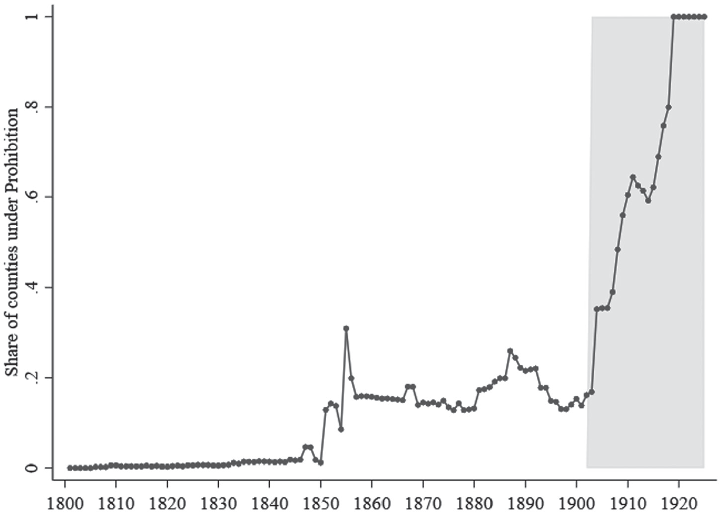
Figure 1 SHARE OF DRY COUNTIES 1800-1925
Notes: The graph shows the share of counties under a dry law for each year 1800-1925. The three shaded areas refer to the three Waves of Prohibition. The figure does not correct for county boundary changes.
Source: Sechrist (Reference Sechrist2012).
This paper focuses on the years from 1900 to 1920, the so-called Third Wave of Prohibition, which corresponds to the period when local and state dry laws experienced rapid expansion.Footnote 12 Most historians credit the success of the Third Wave to the Anti-Saloon League, which was founded in 1893 in Ohio, but soon developed into a national force to the point of assuming the leadership of the temperance movement by the end of the twentieth century (Okrent Reference Okrent2010).
The Anti-Saloon League was rooted in local institutions under the guidance of the national organization. Local churches were fundamental in this effort: the Anti-Saloon League managed to gain the support of those religious denominations in favor of Temperance to the point that it selfdescribed itself as “The Church in Action Against the Saloon” (Anderson Reference Anderson1910). As this quote and the name suggest, while previous instances of the Temperance movement focused on abstention from drinking, the League’s main focus was to restrict access to saloons, which were seen as the chief facilitator of excessive drinking.
The key to the Anti-Saloon League’s success was that it was a singleissue non-partisan movement, willing to support any candidate that would vote to ban saloons. By focusing on a single issue, they were able to build a broad coalition in support of specific dry candidates across party lines (Kerr Reference Kerr1985). This was in sharp contrast to both the Prohibition Party and the Women’s Christian Temperance Union, which in particular had supported numerous social reforms as part of their political project but had failed to make substantial progress on their main reform of interest (Skocpol Reference Skocpol1995).
By focusing on a single issue, the Anti-Saloon League managed to hold together disparate groups who could all get behind the objective of limiting access to the saloon. As Okrent (Reference Okrent2010) notes, “five distinct, if occasionally overlapping, components make up this unspoken coalition: racists, progressives, suffragists, populists… and nativists [emphasis added].” In addition, the Anti-Saloon League was politically savvy and would focus its resources on fighting battles that had a higher likelihood of succeeding: “Study local conditions and reach after the attainable” (as cited in Kerr Reference Kerr1985, p. 95). At the national level, they would push for states to allow counties to have “local options” and work from the local level up if an outright ban was infeasible.
As one might expect from the nativist, racist, and suffragist undertones of the Temperance coalition, Prohibition was more popular among white people, natives, and women. Table 1 shows the coefficients from a Cox survival model exploring how county characteristics relate to adoption. Consistent with the historical narrative and existing evidence (e.g., Lewis Reference Lewis2008), we find that less populous counties, counties with higher shares of whites, females, natives, and people adhering to anti-alcohol religious denominations adopted Prohibition earlier. This is consistent with Strumpf and Oberholzer-Gee (Reference Strumpf2002), who estimate these preferences after the repeal of Federal Prohibition. Importantly, conditional on demographics, economic variables do not help predict the early adoption of Prohibition, as we show in Column (3).
Table 1 CORRELATES OF EARLY ADOPTION

Notes: The table shows the coefficients of a Cox hazard model for when counties become dry. The explanatory variables are county characteristics in 1900. Productivity is defined as log output for the five major crops (corn, cotton, oats, tobacco, and wheat) times 1910 prices per capita. Denomination in favor of Prohibition are Baptist, Evangelical, Methodist/Episcopal, Mormon, and Presbyterian. Railroads is an indicator variable equal to one if the county has railroad access. Standard errors are robust. ***p < 0.01, **p < 0.05, *p < 0.1.
Sources: Prohibition adoption data is from Sechrist (Reference Sechrist2012). Population, share urban, share male, share white, and share immigrant are from the 1900 Population Census. Share in denominations in favor of Prohibition is from the 1890 Census of Religious Bodies. Farm values, implements per capita, share of land in farms, and productivity are from the 1890 Census of Agriculture. Information on railroads is from Atack (Reference Atack2016). Banks data are from Jaremski and Fishback (Reference Jaremski and Fishback2018). See Appendix Table I for more details.
The Effect of Prohibition on Alcohol Consumption, Health, and Crime
The effect of Prohibition on alcohol consumption is still debated. Typically, county dry laws closed down saloons and the production of alcohol but did not involve prohibiting the consumption of alcohol in the home. The effect of Prohibition on alcohol consumption may not have been large for two reasons: many counties in which Prohibition was popular already had high numbers of teetotalers; members at most of the churches behind the Anti-Saloon League would make vows to not drink. In addition, those that did drink were often still able to get alcohol. Until 1913 with the passage of the Webb-Simpson Act, it was legal to ship alcohol across state lines, including states in which alcohol was banned, so it was still available for those that wished to have it for private consumption.
The empirical evidence on consumption is mixed. Data on national alcohol consumption per capita show very little movement between 1900 and 1918, suggesting the effects of local Prohibition did not have much effect on alcohol consumption before federal Prohibition (Miron and Zwiebel Reference Miron1991). Dills and Miron (Reference Dills2004) find that the state dry laws had less than 1 percent effect on cirrhosis from 1910-1920 and less than a 5 percent effect from 1920-1933. However, recent work by Law and Marks (Reference Law2020) that considers the presence of local dry laws finds up to 30 percent lower deaths due to alcoholism in fully dry versus fully wet states. In line with these results, Prohibition appears to have had positive spillovers on children’s health. For example, Evans et al. (Reference Evans, Eric, Jonathan and Ashwin2016) find that exposure to Prohibition in utero increased educational attainment and decreased obesity, while Jacks, Pendakur, and Shigeoka (Reference Jacks, Krishna and Hitoshi2017) find that counties that waited to repeal Prohibition had lower infant mortality than counties that became wet immediately after 1933.
Prohibition might also have affected crime. Owens (Reference Owens2011) finds no overall effects of state dry laws on overall homicide rates, although in Owens (Reference Owens2014) the rates increased for young adults with respect to other age ranges, perhaps in line with higher market-based violence. To the extent that these studies also include the introduction of Federal Prohibition as part of their treatment, it is unclear to what extent we should expect to see the same effect for the local dry laws we are examining, where the incentives to engage in illegal markets were much more limited, and there was likely less tension between the public and law enforcement on the matter. García-Jimeno (Reference García-Jimeno2016) finds that the homicide rate increased after Federal Prohibition and that the increase was larger in cities with stronger wet constituencies. This is also consistent with the idea early supporters of Prohibition might also have seen limited effects on crime.
DATA
County-level data are from the United States Censuses of Population 1880-1920 and Agriculture 1880-1925. We use the official tabulations of the related Census publications, which have been digitized and made available by Manson et al. (Reference Manson, Jonathan, Riper and Ruggles2018) (Census of Population) and Haines, Fishback, and Rhode (2014) (Census of Agriculture). We adjust county- level data to fixed 1920 boundaries following Hornbeck (Reference Hornbeck2010).
We use the Population Censuses to study population, the share of county population living in urban areas, share male, share white, share 1st generation immigrant, and share 1st and 2nd generation immigrant. We supplement the data for outcomes that were not reported in the original tabulations, such as occupation shares for prime-aged men, with our own calculations from a 25 percent sample of the census micro-data from Ruggles et al. (Reference Ruggles2020).Footnote 13
We use the Agricultural Censuses to look at land values per county acre, productivity, value of implements, and share of land in farms. Because land values are not reported separately before 1900, we proxy for land values using farm values, which also include the value of buildings (approximately 20 percent of total farm values). We show in the robustness checks that, if we run the analysis using data after 1900 and define the outcome as the land value per acre, thus excluding the value of buildings, this barely affects our point estimate.Footnote 14,Footnote 15
We use data on county membership of religious organizations from the 1890 Census of Religious Bodies, also available from Manson et al. (Reference Manson, Jonathan, Riper and Ruggles2018), to proxy for baseline preferences for temperance. We divide the different denominations between those in favor of Prohibition (Baptist, Evangelical, Methodist/Episcopal, Mormon, Presbyterian) and against Prohibition (Catholic, Jewish, Lutheran) to define the share of the population in denominations in favor of Prohibition in 1890 following García-Jimeno (Reference García-Jimeno2016). County boundaries are similarly normalized to 1920.
Data on the introduction of Prohibition is from Sechrist (Reference Sechrist2012). The dataset reports information on whether a county was wet or dry yearly from 1800 to 1919, collected from state-specific historical accounts for the earlier period and Prohibition maps published in the Anti-Saloon League after the turn of the century. If only part of a county was dry, for example, if a local option was introduced in a town but not in another, the county is categorized as wet: counties are only classified as dry if their entire territory is under Prohibition. However, in our normalization of county boundaries to their 1920 counterpart, we consider a county as dry if any of the parts constituting the 1920 county were dry to be as conservative as possible.
Finally, data on the number of banks per county are from Jaremski and Fishback (Reference Jaremski and Fishback2018). We define whether a county has access to the railroad network using maps digitized and made available by Atack (Reference Atack2016).
All the data used in the analysis can be found in Howard and Ornaghi (Reference Howard and Arianna2021).
Descriptive Statistics
Table 2 presents the descriptive statistics for the variables used in the analysis for all rural counties that introduced Prohibition after 1900 and separately for early and late adopters. In addition, Appendix Table I provides a summary of how each variable is defined, together with the precise data source used.
Table 2 DESCRIPTIVE STATISTICS

Notes: This table reports descriptive statistics for the main variables considered in the analysis. Columns (1) to (3) restrict the sample to rural counties that adopted Prohibition after 1900 (the sample used throughout the analysis), Columns (4) to (6) restrict the sample to counties that adopted Prohibition before 1910, and Columns (7) to (9) restricts the sample to counties that adopter Prohibition after 1910. Productivity is defined as log output for the five major crops (com, cotton, oats, tobacco, and wheat) times 1910 prices per capita. Denomination in favor of Prohibition are Baptist, Evangelical, Methodist/Episcopal, Mormon, and Presbyterian. Railroads is an indicator variable equal to one if the county has railroad access. All variables are in 1900.
Sources'. Prohibition adoption data is from Sechrist (Reference Sechrist2012). Population, share urban, share male, share white, share 1st and 2nd generation immigrant, and share 1st generation immigrant are from the 1900 Population Census. Share German, Irish, and Italian immigrants and share of males 15-60 in various occupations are calculated from a 25 percent sample of the Population Census 1890-1910. Share in denominations in favor of Prohibition is from the 1890 Census of Religious Bodies. Farm values, implements per capita, share of land in farms, productivity, and share mortgaged are from the 1890 Census of Agriculture. Information on railroads is from Atack (Reference Atack2016). Banks data are from Jaremski and Fishback (Reference Jaremski and Fishback2018). See Appendix Table I for more details.
EMPIRICAL STRATEGY
The empirical strategy estimates the effect of Prohibition by comparing same state counties with similar preferences towards alcohol that introduced dry laws early (1900-1909) and late (1910-1919) in a differences- in-differences design. In 1919, the Volstead Act introduced Prohibition in the entirety of the United States. Because Federal Prohibition was imposed centrally on areas that did not necessarily value it and provided limited enforcement, its effect is likely to be quite different with respect to local adoption in rural areas. As a result, we focus on the effect of local Prohibition, looking at the 1890 to 1910 period. Nonetheless, we explore longer-term outcomes using late adopters as controls in 1920 and 1925 in the event study specification.
The focus of the analysis is the Third Wave of Prohibition, spanning the years between 1900 and 1919. During this period, expansion of dry laws was swift, with the share of dry counties going from 20 to 100 percent over the short span of 20 years: counties in our treated and control group adopted alcohol restrictions only a few years apart. Importantly, the effort was spearheaded by the political efforts of the Anti-Saloon League. The League had a strategy of investing their political and social capital in those places where they thought they could have Prohibition passed first, possibly because of already existing local temperance organizations, and then expand from there to the state and national level. This is suggestive that differences in treatment status for same-state counties with similar baseline preferences for Prohibition likely depended on idiosyncratic differences in whether a window of opportunity opened up a couple of years earlier in a county than in another.Footnote 16
Figure 2 shows the geographic distribution of the treatment. The figure shows that overall the West, Midwest, and Northeast appear to have adopted Prohibition earlier, but there is still significant variation in adoption year within states. Given our focus on the Third Wave of Prohibition, we restrict the sample to counties that were wet in 1899. In addition, we restrict the sample to rural counties, which is the relevant sample for our investiga- tion.Footnote 17 The resulting sample consists of approximately 2,300 counties.

Figure 2 TREATMENT STATUS MAP
Notes: The map shows the treatment status of counties across the United States. Early adopters (treatment group) are counties that introduced Prohibition from 1900 to 1909; late adopters (control group) are counties that introduced Prohibition from 1910 to 1919. We exclude from the sample counties for which there no information about year of introduction of Prohibition (54 counties), counties which adopted before 1900 (412 counties), and urban counties (219 counties). The final sample includes 2,381 counties. The maps shows 1920 county boundaries.
Source: Prohibition adoption data is from Sechrist (Reference Sechrist2012).
The baseline specification we estimate is:
 $${y_{ct}} = \beta 1{(early\,adopter)_c}*\,1{(1910)_t} + {\eta _{bt}}X_{c.1890}^'{\theta _t} + {\alpha _c} + {\alpha _{st}} + {\varepsilon _{ct}},$$
where y ct is outcome y for county c and year t; 1(early adopter) c is a dummy equal to 1 if the county introduced a dry law after 1900 but before 1910; 1(1910)t is a dummy equal to 1 if the year is 1910; q bt are dummies for which decile of the share of the population belonging to denominations in favor of Prohibition in 1890 the county belongs to, interacted with year dummies; X c 1890 are demographic controls according to the 1890 census (population, share urban, share male, share white, share 1st, and share 1st and 2nd generation immigrant), interacted with year dummies; a c are county fixed effects; and a st are state-year fixed effects. Standard errors are clustered at the county level, but we also always report Conley standard errors allowing for spatial correlation in the errors between counties in a radius of 500 kilometers (Conley Reference Conley1999).
The coefficient β estimates the relative change in the outcome in early versus late adopters of dry laws in 1910 after local Prohibition is introduced. The identification assumption is that rural counties that introduced dry laws early in the Third Wave of Prohibition, if not for these laws, would have experienced similar changes in population and farm values as same-state counties with similar Prohibition preferences that introduced them only after 1910. The concern is that late adopters of Prohibition are not a good control group for counties that introduced Prohibition earlier on.
Our preferred specification minimizes endogeneity concerns in a number of ways. First, the fact that we include county fixed effects ensures that any fixed difference across the two groups is considered in the estimation. Second, the inclusion of state-year fixed effects ensures that we are only using a within-state variation. Third, by including dummies for the decile of the share of the population belonging to denominations in favor of Prohibition in 1890, interacted with time dummies, we are comparing counties with similar baseline preferences for Prohibition.Footnote 18 Finally, allowing counties with different baseline characteristics to be on different trends with the inclusion of demographic controls interacted with year dummies further enhances the comparability of the two groups of counties.
However, we might still worry that places that introduced Prohibition earlier did so because they were experiencing different socio-economic changes, to begin with. To take this into account, we additionally estimate the following event study specification for the 1890 to 1925 period:
 $${y_{ct}} = {\sum _\tau }{\beta _\tau }{(early\,adopter)_c} + {\eta _{bt}} + {\theta _t}{X_{c.1890}} + {\alpha _c} + {\alpha _{st}} + {\varepsilon _{ct}},$$
where variables are defined as before and те {1890,1910,1920,1925}. The 1890 coefficients provide an immediate test for pre-existing differences in the two groups with respect to the baseline year. This means that we can use this specification to provide supportive evidence for the identification assumption.Footnote 19 In addition, we use event studies to report coefficients on the longer-term effect of Prohibition. As mentioned earlier in this section, because of the introduction of national Prohibition in 1919 (which was imposed with limited enforcement, and thus likely to imply a quite different “treatment”), we cannot interpret the coefficient in 1920 or 1925 as the causal effect of local Prohibition. Still, we might be interested in the differences between counties in case there is a persistent effect of early adoption of local Prohibition. It is important to note that several states and many counties in our control group enacted local Prohibition between 1910 and 1919, so the reader should not assume that the estimate in 1920 is comparing places with many years of Prohibition to places that only had one year. Rather, it is comparing places that have had Prohibition for more than ten years to places that have had it for less.
Given that our most interesting results are about the local economy, it is reassuring that the Cox adoption model we presented earlier (Table 1) shows the limited predictive power of economic variables, conditional on the demographic controls and state fixed effects. Of the five variables that we group as “economic”—the presence of a railroad, the number of banks per capita, the log of average farm value per acre, the log value of implements per person, the share of land in farms, and the log of productivity—only the log of productivity is marginally significant. Jointly, we cannot reject that all the economic values are zero, suggesting that the treated and control counties have similar economic conditions at baseline.
A related concern to identification is that some other change occurred between 1900 and 1910 that correlated with Prohibition and made counties more attractive and productive. Given that progressives were a key constituency of the temperance movement, we might be particularly concerned about Progressive Era Reforms such as Workers’ Compensation and Mothers’ Pension coinciding with the introduction of dry laws at the county level. A few points are worth noting in this respect. First, Workers’ Compensation and Mothers’ Pension were introduced at the state level and, importantly, mostly during the 1910s (Aizer et al. Reference Aizer, Eli, Ferrie and Lleras-Muney2016; Fishback and Kantor Reference Fishback2007). Moreover, in most states, agricultural workers were excluded from Workers’ Compensation (Fishback and Kantor Reference Fishback2007), thus making the reform less relevant for the rural setting we study. Because reforms at the state level would be controlled for by the state-year fixed effects, and we look at effects starting from 1910, this would not bias our estimates. Second, while the Anti-Saloon League did draw alliances with other movements when it was convenient to do so, it was at heart a single-issue interest group (Okrent Reference Okrent2010) and unaffiliated with any political party (Kerr Reference Kerr1985), which means that it is unlikely that Prohibition was systematically part of large packages of law changes.
Finally, alcohol taxation was a major form of revenue for the government during this time period. Counties that pass dry laws forego this revenue. Data on this is not available at the county level during this time period (Jacks, Pendakur, and Shigeoka Reference Jacks, Krishna and Hitoshi2017). Moreover, this would likely bias our results downward, as higher other taxes or lower public services would lower demand to live in Prohibition counties.
RESULTS
Our results are organized into four parts. First, we show that local Prohibition attracted people and raised farm values. Second, we show that it increased farm labor productivity and especially raised investment in equipment. Third, we show evidence consistent with the hypothesis that the increased productivity is due to increased investment from higher land values. Finally, we show that Prohibition attracted immigrants and African-Americans, a surprising result given the politics of the Temperance Movement.
Prohibition Attracted People and Raised Farm Values in Rural Counties
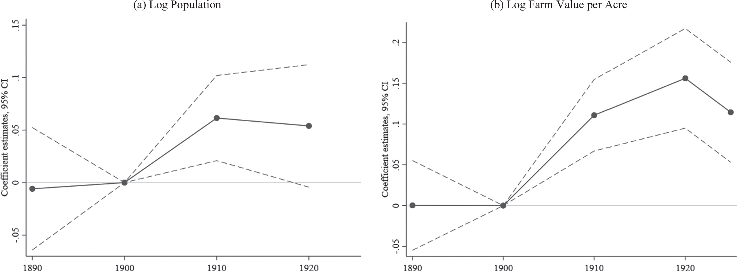
Figure 3 shows the coefficients from the event study specification (Equation (2)), together with 95 percent confidence intervals. Population and farm values, our proxy for land prices, increased in counties that passed Prohibition. This provides evidence for the Tiebout (Reference Tiebout1956) hypothesis that people are willing to move when there are heterogeneous policies in a federal system. It is also consistent with the interpretation that Prohibition was a policy that increased the amenity value of these locations. From 1890 to 1900, there is no economically or statistically different trend for these counties in either population or farm value, showing that the counties were on similar trends. Then, between 1900 and 1910, the population increased by more than 5 percent, and farm values increased by 10 percent in counties that passed local Prohibition. For population, we show that this increase was sustained until 1920. For farm values, we show that it continued to increase from 1910 to 1920, before declining from 1920 to 1925.Footnote 20

Figure 3 PROHIBITION COUNTIES HAVE HIGHER POPULATION AND FARM VALUES
Notes'. The graphs show the effect of Prohibition on population and farm values per county acre by year. Each graph shows the coefficients ß with 95 percent confidence intervals from the event study specification (Equation (2)). We regress the outcome on an indicator variable for being an early adopted interacted with year dummies, deciles of the share of population belonging to denominations in favor of Prohibition in 1890 interacted with year dummies, baseline controls interacted with year dummies, county fixed effects, and state-year fixed effects (Equation (2)). Baseline controls are log population, share urban, share white, share male, share 1 st and 2nd generation immigrant, and share 1 st generation immigrant, all measured in 1890. Population regressions do not control for baseline population. The sample excludes urban counties and counties that adopted Prohibition before 1899. All regressions are estimated by OLS. Standard errors are clustered at the county level.
Sources'. Population is from the Population Census 1890-1920. Farm values are from the Census of Agriculture 1890-1925. Prohibition adoption data is from Sechrist (Reference Sechrist2012). Share in denominations in favor of Prohibition is from the 1890 Census of Religious Bodies. Baseline demographic controls are from the 1890 Population Census. See Appendix Table I for more details.
Table 3 presents the estimates of our baseline specification (Equation (1)), sequentially adding controls. Column (1), which includes no controls, shows positive and large effects. Including controls, especially baseline religiosity in Column (2) and baseline demographics in Column (3), decreases the size of coefficients but also makes our estimates more precise. Our preferred specification is reported in Column (4).
Table 3 EFFECT OF PROHIBITION ON POPULATION AND FARM VALUES

Notes: The table shows the effect of Prohibition on population and farm values per county acre. We regress the outcome on an indicator variable for being an early adopted interacted with an indicator variable for the post period, deciles of the share of population belonging to denominations in favor of Prohibition in 1890 interacted with year dummies, baseline controls interacted with year dummies, county fixed effects, and state-year fixed effects (Equation (1)). Baseline controls are log population, share urban, share white, share male, share 1st and 2nd generation immigrant, and share 1st generation immigrant, all measured in 1890. Population regressions do not control for baseline population. The sample excludes urban counties and counties that adopted Prohibition before 1899, and is restricted to counties for which the outcome is never missing. All regressions are estimated by OLS. Standard errors clustered at the county level are in parentheses and Conley standard errors are in brackets. ***p < 0.01, **p < 0.05, *p < 0.1.
Sources: Population is from the Population Census 1890-1910. Farm values are from the Census of Agriculture 1890-1910. Prohibition adoption data is from Sechrist (Reference Sechrist2012). Share in denominations in favor of Prohibition is from the 1890 Census of Religious Bodies. Baseline demographic controls are from the 1890 Population Census. See Appendix Table I for more details.
The table confirms the event study results: Prohibition increased population by 6.4 percent and farm values by 10.7 percent.Footnote 21,Footnote 22 To put this number in perspective, the standard deviation of population growth rates across all rural counties from 1900-1910 was 46 percent. The five-year interstate migration rate in 1910 was more than 7 percent (Molloy, Smith, and Wozniak Reference Molloy, Smith and Wozniak2011); it may be that Prohibition did not convince people to move, but rather convinced people that were already moving to consider Prohibition in their location decisions.
In Table 4, we show that our results are robust to a number of potential concerns. In Column (1), we windsorize the outcome variable to show that our results do not depend on outliers. Restricting to counties that implemented Prohibition between 1905 and 1915 to only compare counties that adopted Prohibition within a 10-year interval gives very similar, if somewhat smaller, results (Column (2)). Note that this also eliminates counties that did not voluntarily enact Prohibition. Including counties that have missing values for some of the years or using 1900 county boundaries leaves the coefficients virtually unchanged (Column (3) and Column (4)). In addition, as anticipated in the data section, Column (5) shows that focusing on land values (only available after 1900) instead of farm values (which includes the value of buildings but is available for the full period) does not affect the results. This confirms that the effect we observe comes from changes in land values, not building values. Finally, in Appendix Figure II, we explore heterogeneous effects by the share of the population that is rural. There is no effect of Prohibition on population and land values in urban counties, consistent with the idea that Prohibition was a desirable policy change that could impact land values only in rural counties, which supports our sample restriction.
Table 4 ROBUSTNESS CHECKS

Notes: The table shows robustness of the effect of Prohibition on population and farm values per county acre. We regress the outcome on an indicator variable for being an early adopted interacted with an indicator variable for the post period, deciles of the share of population belonging to denominations in favor of Prohibition in 1890 interacted with year dummies, baseline controls interacted with year dummies, county fixed effects, and state-year fixed effects (Equation (1)). Baseline controls are log population, share urban, share white, share male, share 1st and 2nd generation immigrant, and share 1st generation immigrant, all measured in 1890. Population regressions do not control for baseline population. The sample excludes urban counties and counties that adopted Prohibition before 1899, and is restricted to counties for which the outcome is never missing. All regressions are estimated by OLS. Column (1) shows that the main results are robust to winsorizing the outcomes at the 95 percent level. Column (2) restricts the sample to counties that adopted Prohibition between 1905 and 1915. Column (3) includes counties for which we have missing values in certain years. Finally, Column (4) uses 1900 county boundaries. Standard errors clustered at the county level are in parentheses and Conley standard errors are in brackets. ***p < 0.01, **p < 0.05, *p < 0.1.
Sources: Population is from the Population Census 1890-1910. Farm values and land values are from the Census of Agriculture 1890-1910. Prohibition adoption data is from Sechrist (Reference Sechrist2012). Share in denominations in favor of Prohibition is from the 1890 Census of Religious Bodies. Baseline demographic controls are from the 1890 Population Census. See Appendix Table I for more details.
One concern with using a difference-in-differences strategy to study migration is that there are inevitably violations of the stable unit treatment values assumption (SUTVA) as migrants move from an untreated county to a treated county. To that extent, the point estimates should be taken with caution. But given that a gain in the relative amenity value from one area has to be a decline for other areas, the sign of the estimated coefficient is still correct. In Appendix Table III, we show that the results are robust to dropping neighboring counties, which are the most likely to be affected by violations of SUTVA.
Prohibition Led to Higher Farm Productivity and Investments
Next, we show that Prohibition was associated with higher labor productivity and investments. We construct a measure of output from the agricultural census, which provides consistent measures for five major crops (corn, cotton, oats, tobacco, and wheat), covering about 70 percent of total farm production. We use average prices for these five crops in 1910 to get a real measure. We measure farm output by multiplying the quantity of the crop by the price in 1910 and labor productivity as output per person.
Figure 4 shows that counties that adopted Prohibition had large increases in labor productivity, compared to the control counties, conditional on the control variables. The regression estimates from the baseline specification are reported in Table 5. Consistent with the event studies, Column (1) shows that labor productivity increased by approximately 9.2 percent. The effect is significant at the 5 percent level. In Appendix Table IV, we show that this result is robust to different ways of defining the productivity measure.

Figure 4 PROHIBITION COUNTIES HAVE HIGHER PRODUCTIVITY
Notes'. The graphs show the effect of Prohibition on productivity, investments, and banks per capita by year. Each graph shows the coefficients ß with 95 percent confidence intervals from the event study specification (Equation (2)). Productivity is defined as log output for the five major crops (com, cotton, oats, tobacco, and wheat) times 1910 prices per capita. W e regress the outcome on an indicator variable for being an early adopted interacted with year dummies, deciles of the share of population belonging to denominations in favor of Prohibition in 1890 interacted with year dummies, baseline controls interacted with year dummies, county fixed effects, and state-year fixed effects (Equation (2)). Baseline controls are log population, share urban, share white, share male, share 1 st and 2nd generation immigrant, and share 1st generation immigrant, all measured in 1890. The sample excludes urban counties and counties that adopted Prohibition before 1899. All regressions are estimated by OLS. Standard errors are clustered at the county level.
Sources'. Productivity, implements per capital, and share of land in farms are from the Census of Agriculture 1890-1925. Banks data are from Jaremski and Fishback (Reference Jaremski and Fishback2018). Prohibition adoption data is from Sechrist (Reference Sechrist2012). Share in denominations in favor of Prohibition is from the 1890 Census of Religious Bodies. Baseline demographic controls are from the 1890 Population Census. See Appendix Table I for more details.
Table 5 EFFECT OF PROHIBITION ON PRODUCTIVITY AND INVESTMENTS

Notes: The table shows the effect of Prohibition on productivity, investments, and banks per capita. Productivity is defined as log output for the five major crops (com, cotton, oats, tobacco, and wheat) times 1910 prices per capita. We regress the outcome on an indicator variable for being an early adopted interacted with an indicator variable for the post period, deciles of the share of population belonging to denominations in favor of Prohibition in 1890 interacted with year dummies, baseline controls interacted with year dummies, county fixed effects, and state- year fixed effects (Equation (1)). Baseline controls are log population, share urban, share white, share male, share 1st and 2nd generation immigrant, and share 1st generation immigrant, all measured in 1890. The sample excludes urban counties and counties that adopted Prohibition before 1899, and is restricted to counties for which the outcome is never missing. All regressions are estimated by OLS. Standard errors clustered at the county level are in parentheses and Conley standard errors are in brackets. ***p < 0.01, **p < 0.05, *p < 0.1.
Sources: Productivity, implements per capital, and share of land in farms are from the Census of Agriculture 1890-1910. Banks data are from Jaremski and Fishback (Reference Jaremski and Fishback2018). Prohibition adoption data is from Sechrist (Reference Sechrist2012). Share in denominations in favor of Prohibition is from the 1890 Census of Religious Bodies. Baseline demographic controls are from the 1890 Population Census. See Appendix Table I for more details.
The increase in productivity is consistent with increased investment in labor-saving technology. The early twentieth century was a time of increased mechanization. Many of the biggest productivity gains occurred at the end of the nineteenth century, as farms transitioned from manpower to animal power, but new technologies such as improved plows, seed drills, and steam-powered threshers were still spreading to new farms during the time period we study (Rasmussen Reference Rasmussen1962; Manuelli and Seshadri Reference Manuelli2014). Importantly, the technological improvements of this time tended to be labor-saving: “Such devices not only eased the burden of back-breaking labor but also reduced the number of workers and the period of employment for each task” (Atack, Bateman, and Parker Reference Atack, Bateman and Parker2000, p. 261).
Figure 4 shows that early adopters of Prohibition saw the value of implements per capita increase significantly in 1910 and 1920, relative to late adopters. More precisely, Table 5 estimates that Prohibition led to a 9 percent increase in investment in equipment in per capita terms. The share of land devoted to farming also increased but only slightly. Finally, the number of banks increased by more than 0.031 per 1,000 people, which is consistent with the increased demand for credit.
Despite the increase in farm productivity, the share of workers employed in agriculture decreased (Table 6 Column (1)), although the effect is not statistically significant. The negative coefficient is driven entirely by the share of farm laborers (Columns (2) and (3)). The result is consistent with the idea that farm investment is labor-substituting; the addition of equipment on farms allows farms to replace workers.
Table 6 EFFECT OF PROHIBITION ON EMPLOYMENT SHARES

Notes: The table shows the effect of Prohibition on employment shares. We regress the outcome on an indicator variable for being an early adopted interacted with an indicator variable for the post period, deciles of the share of population belonging to denominations in favor of Prohibition in 1890 interacted with year dummies, baseline controls interacted with year dummies, county fixed effects, and state-year fixed effects (Equation (1)). Baseline controls are log population, share urban, share white, share male, share 1st and 2nd generation immigrant, and share 1st generation immigrant, all measured in 1890. The sample excludes urban counties and counties that adopted Prohibition before 1899, and is restricted to counties for which the outcome is never missing. All regressions are estimated by OLS. Standard errors clustered at the county level are in parentheses and Conley standard errors are in brackets. ***p < 0.01, **p < 0.05, *p < 0.1.
Sources: All outcomes are calculated from a 25 percent sample of the Population Census 1900-1910. Prohibition adoption data is from Sechrist (Reference Sechrist2012). Share in denominations in favor of Prohibition is from the 1890 Census of Religious Bodies. Baseline demographic controls are from the 1890 Population Census. See Appendix Table I for more details.
The net effect on the labor market is ambiguous given that productivity increased, but the increase was due to labor-substituting capital. However, note that the decrease in the share of farm laborers was small compared to the population increase, so the total number of farm laborers would still be increasing. In addition, the share of employed workers fell by less and was not statistically significant (Column (4)). This would suggest the labor market boost of increased farm productivity spilled over into other sectors, possibly including manufacturing (Column (5)).Footnote 23
The Land Price Channel
Why did Prohibition have such a large effect on productivity? Our preferred explanation is that the higher land values allowed increased borrowing and investment in capital. This investment raised labor productivity and further increased the population inflows and land values. We highlight the key forces behind this land price channel in a simple model presented in Online Appendix 2.
In the previous sections, we already presented some evidence consistent with this channel: the disproportionate increase in equipment is suggestive of lower capital costs. Here, we show that the effects of Prohibition on farm values, population, and productivity were stronger in areas of the country where this channel would be more likely to be operative. In addition, we use these interactions to help us to distinguish whether the land price channel had any effect beyond any direct effects of Prohibition on productivity.
Our results are presented in Figure 5. To run these regressions, we use the same baseline specification but estimate a separate coefficient for different areas. We also include a dummy control for being in that area.Footnote 24 We begin by investigating heterogeneous effects by access to lending, which we proxy by whether a county is above or below the state median of share of farms mortgaged in 1890 as reported on the Agricultural Census, and the number of banks per capita in 1890 from Jaremski and Fishback (Reference Jaremski and Fishback2018).Footnote 25 The early twentieth century was a time when farmers were becoming increasingly reliant on borrowing. Often, mortgages were taken out in order to invest in the mechanization of the farm (Pope Reference Pope1914). The farm mortgage market was regionally segregated, leading to differences in mortgage rates, and presumably mortgage lending, that was independent of default risk (Snowden Reference Snowden1987; Eichengreen Reference Eichengreen1987).

Figure 5 HETEROGENEOUS EFFECTS BY MORTGAGE SHARE IN 1890, BANKS PER CAPITA, RAILROAD ACCESS, AND SHARE OF BORDER THAT IS ALSO DRY
Notes'. The graphs show heterogeneous effects by mortgage share in 1890, number of banks per capita, railroad access, and share of border that is also dry for population, farm value per county acre, and productivity. The coefficients are estimated in an interacted specifications. We regress the outcome on an indicator variable for being an early adopter interacted with an indicator variable dummy for the post period and with dummies for the group of interest, dummies for the group of interest interacted with year dummies, deciles of the share of population belonging to denominations in favor of Prohibition in 1890 interacted with year dummies, baseline controls interacted with year dummies, county fixed effects, and state-year fixed effects. Baseline controls are log population, share urban, share white, share male, share 1 st and 2nd generation immigrant, and share 1 st generation immigrant, all measured in 1900 and interacted with year dummies. Population regressions do not control for baseline population. The points are the point estimates ß with 95 percent confidence intervals. Standard errors are clustered at the county level.
Sources'. Population is from the Population Census 1890-1910. Farm values, productivity, and share mortgaged are from the Census of Agriculture 1890-1910. Prohibition adoption data is from Sechrist (Reference Sechrist2012). Share in denominations in favor of Prohibition is from the 1890 Census of Religious Bodies. Baseline demographic controls are from the 1890 Population Census. Information on railroads is from Atack (Reference Atack2016). Banks data are from Jaremskiand Fishback (2018). Share of border that is dry is from authors’ calculations. See Appendix Table I for more details.
The results appear to be stronger in places where there was more lending, and therefore an easier way for the land price channel to matter. This is true for population, farm values, and productivity and across the two measures of lending availability. Overall, we think this is suggestive that the land price channel helps explain why Prohibition had large productivity effects.
Next, we look for a different type of heterogeneity based on how much we expect location demand to change. Specifically, counties on railroads were more connected and able to attract migrants. Similarly, places surrounded by wet counties were likely going to be destinations for people that wanted to move into dry counties, more so than places that are already surrounded by dry counties.Footnote 26 Importantly, we also expect that these might be correlated with the availability of alcohol within that county. If we thought Prohibition had a direct effect on productivity, we would expect to see that in places where alcohol was still available in neighboring counties or on a railroad, that the effects on productivity would be smaller. Therefore, this interaction should tell us more than just whether Prohibition was a desirable policy; it will also help us distinguish between two stories about why it might increase productivity.
The results do confirm our interpretation that Prohibition increased the amenity value of these locations. Both population and land prices went up more in railroad-connected counties and counties with relatively more wet borders. They also indicate that the productivity improvements were likely due to the land price channel rather than any direct productivity effects of less drinking, although it is hard to draw strong conclusions from the heterogeneous effects on railroads because of the large standard errors. For the dry border share, there is a much stronger effect in places with more wet borders, which is a natural implication of the land price story because land prices went up more, but the opposite of what a direct effect from the less-drinking story would suggest.
Prohibition Attracted Immigrants and African-Americans
One of our main results is that local Prohibition attracted people. Here, we investigate which people. There are two reasons to do this: first, because it is inherently interesting which groups of people benefit from the policy change, and second because it provides additional evidence on the land price channel.
Some historical context is helpful to understand the intended beneficiaries. Closing the saloon was made the chief goal of the movement, not only because it would diminish temptation, but also because it would thwart the ability of immigrant groups to organize (Sismondo Reference Sismondo2011) and decrease access to alcohol of Southern blacks (see, among others, McGirr (Reference McGirr2015)). According to the Montgomery Advertiser in 1929, “In Alabama, it [was] hard to tell where the Anti-Saloon League ends and the Klan begins” (as cited in Ball Reference Ball1996, p. 61).
Yet, given our previous results on economic effects, it is possible that Prohibition attracted individuals whose preferences might have been not directly aligned with the policy itself but who responded to the potentially higher wages. In addition, these migrants would likely only be attracted by external increases in productivity, like our land price channel, rather than benefits from sobriety. Given that minorities and immigrants were especially mobile, they are particularly likely to be responsive to the changes induced by Prohibition. For example, the timing of Prohibition slightly overlaps with the First Great Migration (Boustan Reference Boustan2009; Derenoncourt Reference Derenoncourt2021), a time when African-Americans were particularly mobile.
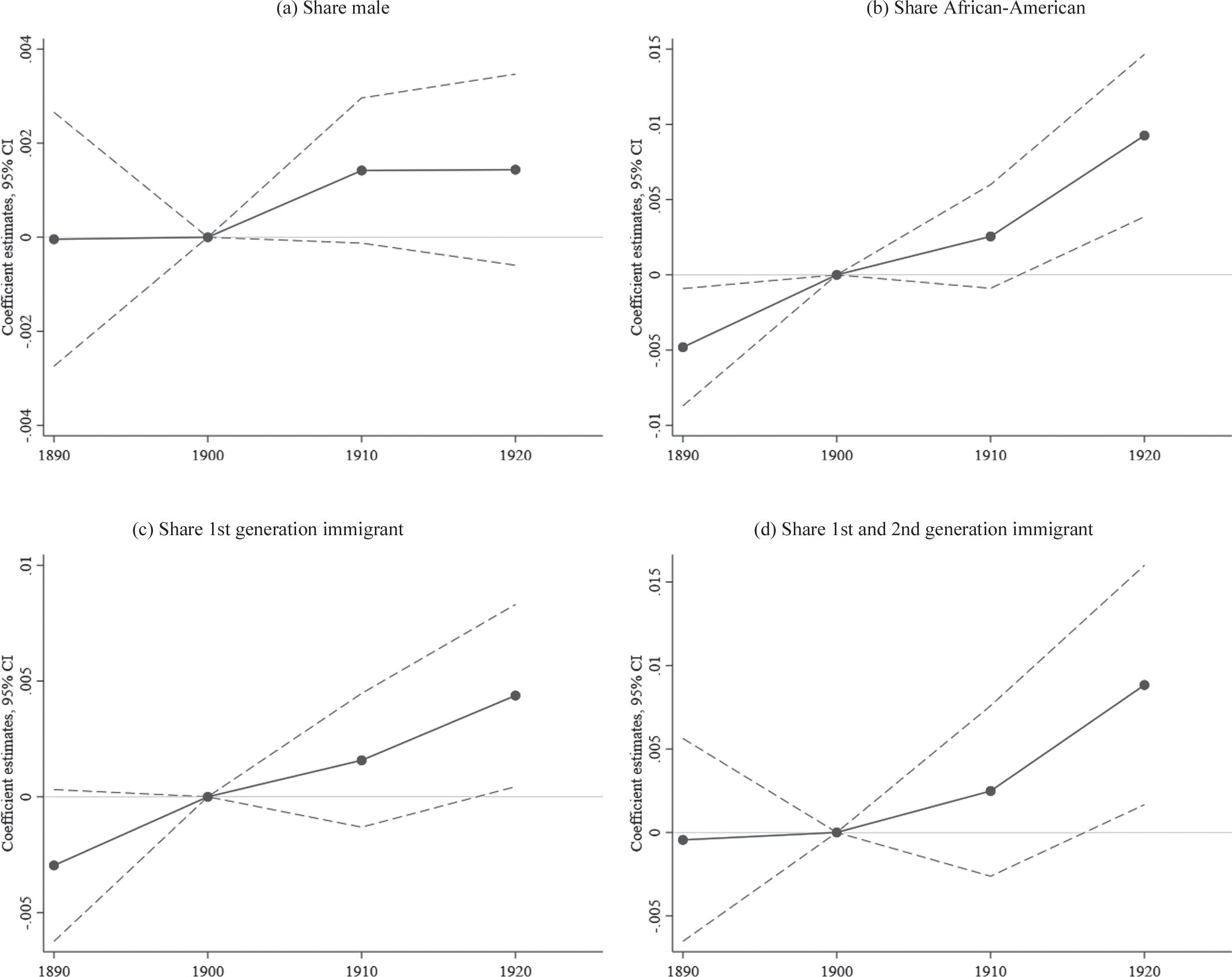
Our event study results are shown in Figure 6, while Table 7 reports the estimates from the baseline specification (Equation (1)). The share of men slightly increased in counties that passed Prohibition, but the effect is not statistically significant in the main specification. The share of African-Americans increased instead by 0.5 percentage points in early-adopting counties after they became dry, with respect to late adopters. To put this number in perspective, the standard deviation of the change in share African-American across counties from 1900-1910 is 2.4 percentage points, so the effect we measure is about a fifth of one standard deviation. Similarly, the share of first-generation immigrants increased by 0.3 percentage points, and the share of first- and second- generation immigrants increased by 0.3 percentage points, although the coefficient is not statistically significant. The standard deviation for these changes is 3 and 4.7 percentage points, respectively. Immigrants who—according to the historical narrative—were particularly opposed to Prohibition, Germans, Irish, and Italians, accounted for most of the gain.Footnote 27,Footnote 28

Figure 6 EFFECT OF PROHIBITION ON SORTING
Notes'. The graphs show the effect of Prohibition on sorting by year. Each graph shows the coefficients ß with 95 percent confidence intervals from the event study specification (Equation (2)). We regress the outcome on an indicator variable for being an early adopted interacted with year dummies, deciles of the share of population belonging to denominations in favor of Prohibition in 1890 interacted with year dummies, baseline controls interacted with year dummies, county fixed effects, and state-year fixed effects (Equation (2)). Baseline controls are log population, share urban, share white, share male, share 1 st and 2nd generation immigrant, and share 1 st generation immigrant, all measured in 1890. In regressions including one of the outcomes, we omit the respective control. The sample excludes urban counties and counties that adopted Prohibition before 1899. All regressions are estimated by OLS. Standard errors are clustered at the county level.
Sources'. All outcomes are from the Population Census 1890-1920. Prohibition adoption data is from Sechrist (Reference Sechrist2012). Share in denominations in favor of Prohibition OO is from the 1890 Census of Religious Bodies. Baseline demographic controls are from the 1890 Population Census. See Appendix Table I for more details. ^
Table 7 EFFECT OF PROHIBITION ON SORTING

Notes: The table shows the effect of Prohibition on sorting. We regress the outcome on an indicator variable for being an early adopted interacted with an indicator variable for the post period, deciles of the share of population belonging to denominations in favor of Prohibition in 1890 interacted with year dummies, baseline controls interacted with year dummies, county fixed effects, and state-year fixed effects (Equation (1)). Baseline controls are log population, share urban, share white, share male, share 1st and 2nd generation immigrant, and share 1st generation immigrant, all measured in 1890. Column (1) excludes share male, Column (2) excludes share white, and Columns (3)-(5) exclude share 1st and 2nd generation immigrant and share 1st generation immigrant from the baseline controls. The sample excludes urban counties and counties that adopted Prohibition before 1899, and is restricted to counties for which the outcome is never missing. All regressions are estimated by OLS. Standard errors clustered at the county level are in parentheses and Conley standard errors are in brackets. ***p < 0.01, **p < 0.05, *p < 0.1.
Sources: All outcomes are from the Population Census 1890-1910, with the exception of share German, Irish, and Italian immigrants that is calculated from a 25 percent sample of the Population Census 1900-1910. Prohibition adoption data is from Sechrist (Reference Sechrist2012). Share in denominations in favor of Prohibition is from the 1890 Census of Religious Bodies. Baseline demographic controls are from the 1890 Population Census. See Appendix Table I for more details.
The event studies for minorities and first-generation immigrants do have borderline significant pre-trends, which raises concerns about whether we identify the causal effect. As a result, these estimates should be taken with some caution. In particular, one story that we are unable to rule out is that Prohibition was passed because of the in-movement of immigrants and African-Americans. For example, in a different time period, Goldin (Reference Goldin, Goldin and Gary1994) argues that increased immigrant populations caused a backlash in policies targeting immigrants. The counties that enacted Prohibition were not places that immigrants had traditionally moved to (see Table 1), but it could be that they begin to move in, and in response, Prohibition is passed.Footnote 29 However, even if that is the case, we still think the event studies presented in Figure 6 are interesting. One might imagine that such policies would be effective at discouraging immigrants, but if anything, it appears to be the opposite, with movements into the counties accelerating after the adoption of Prohibition. Finally, such a story should not concern us with interpreting the economic outcomes causally. The number of immigrants is small both before and after the shock, and the magnitudes would not be able to account for such large changes in productivity and investment.
While the magnitudes of our estimates are small, the particularly interesting part is the signs. Prohibition’s supporters tended to be female, white, and native, so it is unlikely that these results are due to the heterogeneous preferences for the policy. Rather, these groups are also most likely to benefit from increased farm labor productivity. It supports the land price channel because increased productivity due to sobriety would have been available to them in any location, but increased productivity due to higher investment would be specific to a location.
The sorting of workers might also have amplified the effects on productivity, as the groups moving in may have had higher farm productivity. However, attracting these groups was probably not the initial cause of the increased productivity, as these groups valued the policy less. So while we think this sorting may have amplified the channels discussed previously, we still think the evidence points to the land price channel as the initial cause.
Finally, it is important to note that the magnitudes of our sorting results do not imply that women, natives, and whites were moving out of areas that imposed Prohibition. In fact, combining this with our results on population would imply that the number of people of all groups rose because of Prohibition. But we wish to stress the fact that these were disproportionately immigrants and African-Americans.
CONCLUSION
In this paper, we investigated the equilibrium effects of a prominent policy, the U.S. Prohibition. Our results are consistent with the interpretation of Prohibition as a policy that increased amenity values: land prices and population increased and did so more in areas that were connected via railroad or that were surrounded by counties without Prohibition. Prohibition increased productivity, and we present evidence that this was due to a land price channel. We also show evidence that sorting occurred in a counterintuitive way: the groups that most preferred Prohibition actually decreased as a share of the population. So while there does seem to have been a lot of migration in response to heterogeneous policies à la Tiebout (Reference Tiebout1956), the direction of sorting was not always intuitive.
The various causal relationships between sorting, productivity, land prices, and amenities have been the subject of many studies (e.g., Glaeser, Kolko, and Saiz Reference Glaeser, Jed and Albert2001; Florida Reference Florida2003). Here, we are able to document a new channel that positive amenities cause higher land prices that cause higher productivity that cause a higher share of low-skilled workers. To our knowledge, this has not been previously documented. The existing literature has focused on the effects of amenities affecting sorting either directly or through land prices and usually finds sorting toward high- skilled workers (Diamond Reference Diamond2016). Our paper shows that in at least one setting, policies affecting amenities encouraged sorting towards low- skilled groups. More generally, we have shown that it is important to pay attention to the land price channel on productivity when considering the sorting effects of local policies in a federal system.
Supplementary material
For supplementary material accompanying this paper visit https://doi.org/10.1017/S0022050721000346