


1. Introduction
Population aging poses a major challenge to the social security system in all the Organization for Economic Co-operation and Development (OECD) countries. While aggregate public pension and health care expenditures are expected to rise strongly, future GDP growth may fall. Belgium is no exception to the phenomenon of aging. As in other countries, fertility has gradually declined throughout the twentieth century. This downward trend was interrupted only during the period of the baby boom in the 1950s and 1960s. At the same time life expectancy has increased enormously. Together with the retirement of the baby boom generation since about a decade and the reduced size of more recent generations, the structural increase in life expectancy will imply a drastic change in the age distribution of the Belgian population in the period 2010–2040. As we show in Figure 1, the age dependency ratio, computed as the number of people younger than 18 or older than 64 relative to the population at working age, is expected to rise from about 60% in 2010 to an unprecedented 80% by 2040. Figure 2 depicts the evolution of the size of the underlying three age groups. Changes in the number of children reflect changes in fertility. While the number of people older than 64 rises rapidly, the Belgian population at working age is expected to decline between 2020 and 2040. By 2040 there will be eight dependent persons for every ten people at working age.

Figure 1. Age dependency ratio in Belgium (%).
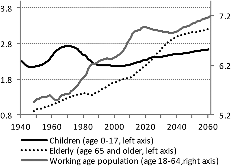
Figure 2. Size of three age groups (millions). Data sources: Federal Planning Bureau, Population forecasts 2015–2060, March 2016; Belgian Federal Government (FPS Economy, Statistics Belgium).
Without behavioral changes in labor supply, education and savings, which may all affect investment in physical capital, this demographic transformation will certainly cause a significant loss in per capita output and income. As a matter of simple arithmetic, if fewer active people are available to produce output for more dependent people, and no one changes his or her behavior, lower per capita output is unavoidable [Onder and Pestieau (Reference Onder and Pestieau2014)]. Fortunately, individual behavior can change. A large theoretical literature has demonstrated that falling fertility and increasing life expectancy (aging) will also affect the incentives for individual households and firms to work, to save, and to invest in human and physical capital. At least four major questions remain, though: (i) Will these incentives go in the right direction? The literature remains ambiguous; (ii) If they go in the right direction, will they be strong enough to reverse the negative effects of demographic transformation on per capita output? (iii) Given that not everyone has the same abilities and/or chances to study or work, what will be the impact of demographic change and the induced behavioral responses on income inequality and unemployment? (iv) What is the impact of the underlying components of demographic change (reduced fertility versus increasing life expectancy)?
To the best of our knowledge, the existing literature does not yet provide clear and comprehensive quantitative answers to this set of questions. In a recent survey article, Lee (Reference Lee, Piggott and Woodland2016, p. 110) qualifies these or highly similar questions as to be explored furtherFootnote 1. Our objective and the main contribution of this paper is to answer these four questions for Belgium, a small open European economy. We focus on one particular country that we know well. This also seems by far the most realistic way to proceed, given the importance of taking into account country-specific structural and institutional characteristics and the need for quantitative answersFootnote 2. It goes without saying, though, that our approach can also be adopted to study other (small) open economies.
To obtain the answers to our questions, several steps need to be taken. First of all, a rich and realistic parameterized model of the Belgian economy will be necessary. We construct this model in the first part of this paper. It will be a 28-period overlapping generations model for an open economy, facing an exogenous world interest rate, that we calibrate to Belgium. Next to its overlapping generations setup, its main characteristics are the following. First, fertility and life expectancy are exogenous but time-varying. Second, hours worked, human capital and income are all endogenous, which implies the capacity of the model to capture and measure important behavioral responses to aging. Third, as to the sources of inequality in the model, individuals differ not only by age but also by innate ability. We distinguish individuals with either high, medium or low ability. Individuals with higher ability enter with more human capital. They are also more productive in building additional human capital and skills when they allocate time to education. For individuals with low ability, expanding time in education is not a productive option. Furthermore, while the labor market for high and medium ability individuals is perfectly competitive and clears, above market-clearing wages imply (involuntary) unemployment among low ability individuals. The introduction of different ability types and unemployment is a second contribution of this paper to the literature. Whereas recent models like those developed by e.g., Ludwig et al. (Reference Ludwig, Schelkle and Vogel2012), Attanasio et al. (Reference Attanasio, Bonfatti, Kitao, Weber, Piggott and Woodland2016) and Marchiori et al. (Reference Marchiori, Pierrard and Sneessens2017) focus on the intergenerational dimension of the impact of population aging, our model also allows an analysis of the intragenerational dimension. Last but not least, our model includes a rich specification of fiscal policy. At the revenue side, the government can change (progressive) tax rates on labor, capital, and consumption. At the expenditure side, it can change non-employment benefits for involuntarily unemployed workers and government purchases of goods and services. It can also allocate resources to maintain financial balance in the public pension system, if necessary. The latter is modeled as a pay-as-you-go (PAYG) system of the defined benefit type.
As a second step, before we use the model for simulations of the future, it should convince in its capacity to replicate the evolution of key data in the past. We, therefore, relate the calibrated model's predictions for the old-age dependency ratio, per capita growth, capital formation, employment, education, and inequality to the data in Belgium since about 1960. We find that the model performs well in this respect. Our third step is the computation of our baseline simulation. This simulation quantifies the effects of projected future demographic change on the endogenous variables in our model until 2061, under the assumption of unchanged policies and under the main rules of the current pension system. Major attention will go to our predictions for future per capita growth, its underlying determinants (employment, physical capital formation, education, and human capital formation), and income differences between low and high ability individuals. Counterfactual simulations will allow us to assess the impact of the separate components of demographic change.
Our predictions are not optimistic. Arithmetically, i.e. for unchanged household and firm behavior, projected demographic change may cut off about 0.4%-points on average of the annual per capita growth rate in the next 25 years. Although we do observe sizeable (and mostly positive) behavioral adjustments by households and firms to the demographic transformation, their effects can only partially counteract the unfortunate arithmetical consequences of the rapidly increasing dependency ratio. A net negative effect on future annual per capita growth of 0.29%-points remains. The reasons are multiple. First, some of the behavioral responses are negative, in particular the response of private investment in physical capital. Private investment suffers mainly from the negative effect on the productivity of physical capital induced by reduced fertility and a declining population at working age. Second, the strong increase in savings that we also observe cannot counteract this negative effect: in an open economy these savings may also be invested abroad (capital outflow). Third, some of the positive behavioral adjustments have already taken place in previous decades.
Decomposing the behavioral responses and their growth effects according to the separate components of demographic change, it is clear from our results that the main problem is reduced (low) fertility after the baby boom. This has not only resulted in a reduced population at working age, with negative effects on investment in physical capital, the retirement of the baby boom generation is now also a major factor behind the growing share of retirees. The induced behavioral effects from rising life expectancy are broadly positive and almost strong enough to compensate for the quantitative effect of longer life spans on the number of retirees.
Our findings on the income distributional effects of demographic change are nuanced. The capacity of individuals with a high ability (and income) to respond to increasing life expectancy by building more human capital, and by saving more, are clearly forces that lead to higher income inequality. To some degree, individuals of low ability may counter these forces by working more hours, but this then goes at the cost of their leisure and welfare. As to unemployment among low ability individuals, we find no noticeable impact of demographic change. Last but not least, our results highlight the major role of the pension system for inequality. If pensions do not follow wages, a rapidly rising share of elderly people will be another important force to higher income inequality.
Our results also contribute to the recent literature on secular stagnation. In line with Gordon (Reference Gordon, Teulings and Baldwin2014) and Cervellati et al. (Reference Cervellati, Sunde and Zimmermann2017), we provide evidence supporting the hypothesis that the observed and expected long-run slowdown in per capita growth is mainly a supply-side problem, with demographic change as one of the main “headwinds.”
The structure of this paper is as follows. In section 2, we assess the arithmetical effects on per capita growth of projected demographic change in Belgium in comparison to other European countries. We also give a brief overview of the potential behavioral responses of households and firms to demographic change, as discussed in the literature. Section 3 sets out the model. In section 4, we describe our calibration procedure and the parameterization of the model. Section 5 demonstrates our model's capacity to replicate the evolution since about 1960 of key macro variables. In section 6, we report our baseline and counterfactual simulation results on the macroeconomic effects of (separate components of) demographic change until 2061. Section 7 discusses income distributional effects across ability groups. Section 8 concludes the paper.
2. Demographic change and aging: unfortunate arithmetic and behavioral effects
In the neoclassical framework that we adopt in this paper, the long-run per capita growth rate is determined solely by the exogenous rate of technical progress. In long transition periods, however, per capita growth can be much higher or much lower than technical progress. Demographic change is a prominent possible cause of such growth deviations. Consider the following decomposition of per capita output

where Y t/Hourst is real output per hour worked (or labor productivity), ${\rm Hour}{\rm s}_t/N_t^w$ hours worked per person at working age and $N_t^w /{\rm Po}{\rm p}_t$
 the share of people at working age in total population. Taking growth rates, it then follows that

The left side of this equation is the annual per capita economic growth rate. On the right, g π is the annual growth rate of labor productivity, n pop the growth rate of total population, n hours the growth rate of total hours worked, and $n_N^w$ the growth rate of population at working age. As can easily be seen, demographic change pushes per capita growth below the growth rate of labor productivity when total population grows faster than population at working age (=rising dependency, $n_{{\rm pop}} \gt n_N^w$
 ) and/or when population at working age grows faster than aggregate hours worked (=falling employment rate, $n_{{\rm hours}} \lt n_N^w$
 ). In the very long run, dependency and employment rates will be constant, and labor productivity and per capita output will grow at the same rate as technology. In long transition periods, however, things may be very different. Figure 1 showed us the evolution of the past and projected future overall dependency ratio in Belgium. Figure 3 reports the arithmetical effects of this changing dependency on per capita growth. We compare Belgium to a few other countries and the European average. Ceteris paribus, the projected unprecedented rise in the dependency ratio between 2010 and 2040 will have significant adverse effects on future per capita growth. In the next 25 years it may cut off almost 0.4%-points on average from annual per capita growthFootnote 3. Compared to other countries, Belgium takes an intermediate position. In Germany and in the EU28 on average the negative arithmetical effects of rising dependency are larger (about 0.5%-points on average in the next 25 years). They are weaker in a country like Sweden (about 0.2%-points). In all countries, and Germany in particular, these negative arithmetical effects are the strongest in 2020–2035.
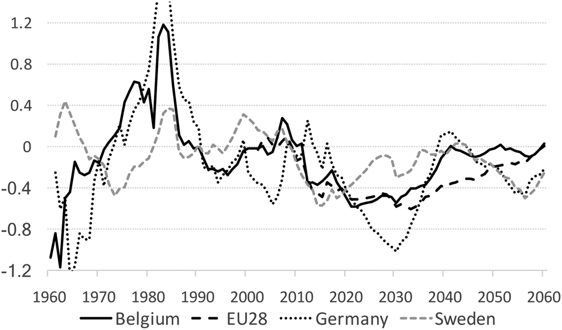

The negative effects of a rising dependency ratio on per capita growth can be countered if countries succeed in raising hours worked among the smaller group of people at working age or the growth rate of labor productivity (output per hour). Despite some progress in the second half of the 1990s, Belgium is one of the countries with the poorest labor market performance (Figure 4). Moreover, in the last decade, per capita hours worked have again stagnated. The employment gap between Belgium and other countries is particularly large for older workers and low-skilled workers [OECD (2015)]. At the same time, this gap also creates huge opportunities to counter low per capita growth if Belgium manages to mobilize this enormous amount of non-employed labor. As to the growth rate of labor productivity, Belgium also lags behind other countries. In 1996–2016 the annual growth rate of real GDP per hour worked in Belgium was 1%. In the EU28 it was 1.3% [OECD.Stat, Productivity database (2017)].
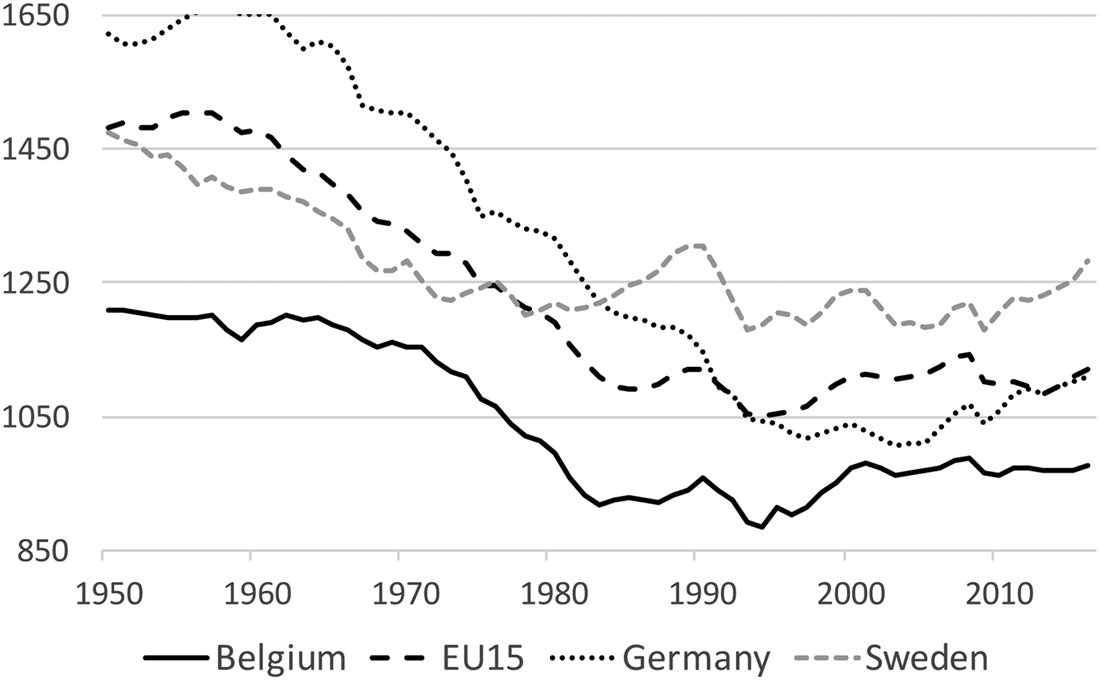
Figure 4. Average annual hours worked per person at working age.
The effects of demographic transformation on per capita growth in the medium to long run are not limited, however, to the arithmetic described above. Demographic change also implies a change in the structure of the population, and thus in the relative size of different age groups with different behavior. Moreover, and maybe more important, demographic change will also affect the incentives for individual households to supply labor, to invest in human capital, and to save. Likewise, it will affect the incentives for firms to hire workers and to invest in physical capital. Changes in investment behavior will affect labor productivity. It is unclear from the literature, however, whether the net effect of all these incentives will be positive for growth or negative. And if it is positive, whether it will be strong enough to reverse the arithmetical effect shown in Figure 3.
When it comes to aggregate savings, there are reasons that can justify a decline in response to demographic change, as well as reasons that would predict an increase. Whereas middle-aged and older workers are net savers, young people and (old) retirees are generally described as borrowers or dissavers. Considering the demographic transition in Figure 2, the obvious expectation would be that aggregate savings will gradually be declining as the rising share of dependent versus active people should soon feed through in a rising fraction of dissavers [see e.g., Goodhart and Erfurth (Reference Goodhart and Erfurth2014), IMF (2014)]. Increasing life expectancy, however, may imply the opposite. Individuals prefer to smooth consumption over their whole lifetime. The perspective of living longer may then force them to increase their savings during their active life [Krueger and Ludwig (Reference Krueger and Ludwig2007), Onder and Pestieau (Reference Onder and Pestieau2014)]. A key element determining the extent to which this will happen is the retirement decision and the length of working life. The ambition to maintain consumption during old age will also provide an incentive for individuals to work longer and to postpone retirement, at least if good health and productivity can be assumed [Bloom et al. (Reference Bloom, Canning, Mansfield and Moore2007), Heijdra and Reijnders (Reference Heijdra and Reijnders2018)]. The stronger the reaction in labor supply, the smaller will be the need to increase savings at middle age.
Increasing life expectancy does not only provide an incentive to work longer. It will also increase the incentive for individuals to invest in education, at least if they have the ability to do so. The reason is obvious. If people expect to live longer—starting with reduced mortality during normal working ages—and if they expect to work longer, accumulated human capital will be productive for a longer period of time. All this raises the return to investment in education [Ben-Porath (Reference Ben-Porath1967), Ludwig et al. (Reference Ludwig, Schelkle and Vogel2012), Cervellati and Sunde (Reference Cervellati and Sunde2013), Heylen and Van de Kerckhove (Reference Heylen and Van de Kerckhove2013)].
The response of individuals regarding saving, working and schooling, will matter a great deal for firms' investment in physical capital. For given (constant) individual behavior, demographic change will most likely imply disinvestment. If fertility and the size of working-age population decline, this will cause an increase in the capital-labor ratio and reduce the marginal productivity of physical capital. The lower rate of return to physical capital may then lead to a fall in investment [Ludwig et al. (Reference Ludwig, Schelkle and Vogel2012), Heylen and Van de Kerckhove (Reference Heylen and Van de Kerckhove2013)]Footnote 4. If individuals adjust their behavior, however, the outcome may be very different. An increase in savings may push down the interest rate and reduce the cost of investment. Increased labor supply and/or postponement of retirement, and increased accumulation of human capital will raise the marginal productivity of physical capital, and counteract the negative effect of a decline in population aged 18–64. An important element here is the extent to which the interest rate can indeed fall. Given our focus on Belgium, we model in this paper an open economy. A fall in the interest rate and an increase in domestic investment are then not obvious, as savings may simply be invested abroad (capital outflow). This will be the case if the rate of return to physical capital abroad is higher than at home. In the end, what matters is relative aging in the home economy versus abroad, as well as the relative response of labor supply and schooling.
If one thing is clear from this discussion, it is that demographic change affects household and firm behavior in many ways. Uncovering overall net effects on the macro economy will require a coherent general equilibrium model. It is our aim to construct this model in section 3.
3. The model
We assume an open economy with an exogenous but time-varying world interest rate. Physical capital moves freely across borders. Human capital and labor, however, are assumed internationally immobile. Time-varying exogenous fertility and survival rates drive demographic change. Twenty-eight generations of individuals coexist. Individuals enter the model at the age of 18. They live at most for 28 periods of 3 years. Within each generation one fraction of the individuals is assumed to have low innate ability, others have medium ability, a third group has high innate ability. Depending on their ability, individuals will enter the model with a different initial human capital endowment and with a different productivity of schooling. Young individuals with high or medium ability will continue education when they enter the model at 18. Individuals with low ability will not. The introduction of differences in individuals' ability and productivity of schooling is a new element compared to existing models to study the economic effects of demographic change [see e.g., Ludwig et al. (Reference Ludwig, Schelkle and Vogel2012), Attanasio et al. (Reference Attanasio, Bonfatti, Kitao, Weber, Piggott and Woodland2016), Marchiori et al. (Reference Marchiori, Pierrard and Sneessens2017)]. It also allows an analysis of the intragenerational dimension of these effects. Next to endogenous education and human capital, our model also has endogenous employment. Besides studying (for high and medium ability individuals) everyone optimally allocates time to labor and leisure. The labor market for high and medium ability households is assumed perfectly competitive. The labor market for low ability households is imperfectly competitive. We assume the existence of a union that sets wages for low ability workers. Above market-clearing wages may cause involuntary unemployment. As to output, domestic firms are modeled to employ physical capital and effective labor under constant returns to scale. Technology is assumed to have exogenous growth. The government in our model sets tax rates on labor (both on employees and employers), consumption, and capital income. It allocates its resources to goods and services, non-employment benefits and pensions (to finance possible deficits in the public pay-as-you-go system). It may also borrow.
Concerning notation, superscript t denotes the time an individual or group of individuals (a generation) enter the model. Subscript j refers to the j-th period of life or, differently put, the age. It goes from 1 to 28Footnote 5. When a subscript s is used, it denotes one of three levels of innate ability: low (L), medium (M) or high (H). Last but not least, time subscripts t added to aggregate variables indicate historical time.
3.1 Demography
Demographic change in our model is captured by the evolution over time of fertility and survival rates, with the latter determining individuals' expected length of life. Equation (1) expresses the size of the youngest or “newborn” generation at time t relative to the size of the youngest generation at t−1, following among others de la Croix et al. (Reference de la Croix, Pierrard and Sneessens2013). f t(>0) is the time-dependent “fertility” rate in the model.

Equation (2) describes the evolution of the size of a specific generation over time. We denote by $sr_{j-1}^t$ (<1) the probability for each individual of generation t to survive until model age j conditional on reaching age j − 1. This survival rate is both generation and age-dependent.

The trajectories of both f t and $sr_j^t$ are taken as exogenous in our modelFootnote 6. Figures 5a and 5b show the data. Finally, the population consists of low, medium, and high ability agents:

with v s denoting their respective shares and $\sum_{s = L,M,H}v_s = 1$ . Assuming the fertility and survival rates to be equal across ability types, these shares will be constantFootnote 7.

The fertility rate f t in Figure 5a is computed as the ratio of the size of the population of actual age 18–20 in a particular 3-year period to its size 3 years earlier. We observe a peak in 1963–65 and 1966–68, when the after-war baby boomers became 18. Both periods reveal a growth rate of the youngest generation by almost 20% compared to the previous period. After a few more periods with f t > 1 in the 1970s, we observe a decline of the youngest generation (f t < 1) in the 1980s and 1990s. Later decades show a pattern of dampened oscillation. Figure 5b shows the evolution over time of conditional survival rates, $sr_j^t$ , for individuals born in 1905, 1925, 1950, 1975, and 2014. We observe an overall rise, with higher probabilities to survive at higher age, for people born later. The increase is particularly strong at ages 75 and 90. A child born in Belgium can now (unconditionally) expect to reach age 90 with a probability of more than 60%. For a child born in 1950 that probability was less than 30%.
In line with our assumption that only physical capital is internationally mobile, we do not model migration in this paper. Our data for the exogenous fertility rate do, however, capture the impact of migration of individuals not older than 20. The data also count the children of migrants when these children reach age 18–20 (model age 1)Footnote 8.
3.2 Households
Individuals of the same generation and ability are grouped in a representative household of unitary mass [Merz (Reference Merz1995), Andolfatto (Reference Andolfatto1996), Boone and Heylen (Reference Boone and Heylen2019)]. As low ability individuals can be involuntarily unemployed, their household will consist both of a fraction of unemployed (u) and a fraction of employed members (1 − u). They pool their income, so consumption is equalized across household members. Medium and high ability households have only employed members.
3.2.1 Instantaneous household utility
The instantaneous utility function of a representative high or medium ability household of age j born at time t depends positively on consumption $c_{j,s}^t$ and leisure time $l_{j,s}^t$
 (equation 4). Preferences are logarithmic in consumption and iso-elastic in leisure. The intertemporal elasticity of substitution in leisure is 1/θ. Furthermore, γ j indicates the relative utility value of leisure versus consumption. It may differ by age. The instantaneous utility function of a low ability household of age j is the same except that only the leisure time of the employed fraction of the household (1 − u t+j−1) is taken into account (equation 5). Implicitly, leisure of the unemployed fraction is assumed to be neutral for household utility.


with γ j > 0 and θ > 0 (θ ≠ 1).
3.2.2 Expected lifetime utility
A household that enters the model at time t maximizes expected lifetime utility described by equation (6) subject to its budget and time constraints (cf. infra). In this equation β is the discount factor and $\pi _j^t$ the unconditional probability to survive until age j.

with 0 < β < 1, $\pi _1^t = 1$ , $0 \lt \pi _j^t = \prod \nolimits_{i = 1}^{j-1} sr_i^t \lt1$
 for 1 < j < 29, and $\pi _{29}^t = 0$
 .
.
3.2.3 Time constraints
Every period, an individual is endowed with one unit of time that can be split into hours worked while employed (n), education (e) and leisure (l) depending on age and innate ability. Equations (7) to (9) describe the age-dependent time constraints for medium and high ability individuals (s = M, H). Only in the first 4 periods an individual can spend time in post-secondary education next to working and enjoying leisure. From period 5 until 15, time can exclusively be allocated to labor and leisure. From period and age 16 onwards an agent is eligible for public old-age pensions.


Equations (10) and (11) relate to low ability individuals. Since these individuals start working earlier than individuals of medium or high ability, they can also leave the labor market earlier. They receive a public pension from period and age 15 onwardsFootnote 9. Unemployed low ability individuals cannot choose hours worked or leisure (for them $n_{j,L}^t = 0$ ). They only have “leisure”. As mentioned before, this does not carry positive utility.


3.2.4 Budget constraints
Households have varying budget constraints over their life cycle depending on age and innate ability. Equation (12) describes the budget constraint faced by households of high and medium ability during active life (periods 1–15).

Disposable income is used to consume $c_{j,s}^t$ and accumulate non-human wealth. We denote by $a_{j,s}^t$
 the stock of wealth held by a type s individual at the end of the j-th period of his life. τ c is the tax rate applied by the government on consumption goods. When individuals assign a fraction $n_{j,s}^t$
 of their time to work, with productive efficiency $\varepsilon _jh_{j,s}^t$
 , they earn a net labor income of $w_{t + j-1}^s \varepsilon _jh_{j,s}^t n_{j,s}^t \lpar {1-\tau_{w,j,s}} \rpar$
 . Underlying factors are the real gross wage per unit of effective labor of ability type s ($w_{t + j-1}^s$
 ), an exogenous parameter linking productivity to age (ɛ j), human capital ($h_{j,s}^t$
 ), and the average labor income tax rate (τ w,j,s). The contribution rate cr 1 of workers to the public pension system is included in τ w,j,s. Engaging in work, however, also induces costs related to child care and transportation T j,s. Moreover, if the individuals in a household work more days a week and more weeks per year, implying higher n, these costs will rise. This explains why we have $T_{j,s}n_{j,s}^t$
 in the budget constraint. One reason for T to depend on ability is for example the use of company cars, which make transportation cheaper typically for higher ability individuals. A reason for T to depend on age is the need (to pay for) for child care at low j, when households have children.
Next to labor income, disposable income consists of interest income earned on assets, $r_{t + j-1}a_{j-1,s}^t$ with r t+j−1 the exogenous world real interest rate, and lump-sum transfers received from the government z t+j−1. A final source of income are transfers from accidental bequests tr t+j−1 (plus interest). There are no annuity markets in our model. Transfers are uniformly distributed among the population (N k):

From the eligible pension age j = 16 onwards individuals of high and medium ability receive public pension benefits $ppt_{j,s}^t$ (see also section 3.3). Equation (13) presents these individuals' budget constraint.

The budget constraint of low ability households at working age (equation 14) looks slightly different. Here, only the employed fraction of the representative household (1 − u t+j−1) earns a labor income while the unemployed part receives an unemployment benefit related to what they would have earned when employed. The policy parameter b indicates the gross benefit replacement rate.

After retirement (from age j = 15 onwards) the budget constraint of low ability households is the same as the one of high or medium ability households.

All households in our model are born without assets. They also plan to consume all accumulated assets by the end of their life. A final assumption is that retired individuals cannot have negative assets. Algebraically, $a_{0,s}^t = a_{28,s}^t = 0$ and $a_{j,s}^t \ge 0$
 for j >15 (for s = H, M) or 14 (for s = L).
3.3 The pension system
Our model includes a public pay-as-you-go (PAYG) pension scheme of the defined benefit type that makes pension payments to retirees out of contributions (taxes) paid by current workers and firms. Individuals receive a pension benefit from model age j = 16 (for s = H, M) or j = 15 (for s = L) onwards, i.e., respectively actual age 63 or 60. The amount $ppt_{j,s}^t$ they receive at the time of retirement is

or

The pension benefit is related to one's own contributions during active life. More precisely, the pensioner receives a fraction of the average of revalued earlier net labor income. In equation (16), rr s is the net replacement rate, which can differ by ability (income), and wg is the period-wise revaluation factor applied to net labor income earned in the past. The pension will rise in the earned wage, the individual's hours of work and his productive efficiency with the latter also increasing in human capital. For retired low ability households the pension amount looks very similar, except for the lower eligibility age of 60 (model age 15). Underlying this, is our assumption that periods of unemployment, as experienced by some household members, are considered equivalent to periods of workFootnote 10.
After the initial pension payment, the pension benefit may be revalued to adjust for a changed living standard, so $ppt_{j,s}^t$ then becomes


with pg k the coefficient that revalues the pension benefit of period k − 1 to k Footnote 11.
The public pension system's budget identity is as follows:

with cr = cr 1 + cr 2.
The left side of equation (18) indicates total pension expenditures at time t. As public pensions are organized on a PAYG basis, this amount is financed by (a) the working population from taxes on their gross labor income applying contribution rate cr 1 and by (b) the firms applying cr 2. In equations (12) and (14), cr 1 is thus part of the labor tax rate τ w,j,s. Tailored to institutional reality in Belgium, GPP t denotes the total resources assigned to pension payments by the government to ensure that equation (18) holds.
3.4 Human capital production
Individuals enter the model at the age of 18 with a predetermined ability-specific endowment of human capital. In equation (19), h 0 stands for the initial time-invariant human capital endowment of a high ability individual. Low and medium ability individuals are respectively endowed with lower human capital stocks ω Lh 0 and ω Mh 0 with 0 < ω L < ω M < ω H = 1.

High and medium ability individuals can engage in higher education to accumulate additional human capital in the first four periods (equation 20a). ϕ s is a positive ability-related efficiency parameter reflecting the productivity of schooling, and σ the elasticity of human capital growth with respect to time input. After the first four periods, human capital remains constant (equation 20b). We assume that learning-by-doing offsets depreciation. Constant human capital, however, does not imply constant productive efficiency $h_j^t \varepsilon _j$ , as there is still variation in the exogenous age-productivity link ɛ j.


with: 0 < σ < 1, ϕ H, ϕ M > 0.
Individuals with low innate ability do not study at the tertiary level. Their human capital remains constant at the initial level:

3.5 Household optimization
Low ability individuals will choose consumption and labor supply to maximize equation (6), taking into account their instantaneous utility function (equation 5), their time and budget constraints (equations 10, 11, 14 and 15) and the human capital process (equations 19 and 21). Individuals of medium and high ability will in addition choose the fraction of time they spend in education when young. They optimize equation (6), taking into account equation (4), and their time and budget constraints and the human capital formation process described by equations (7)–(9), (12), (13), (19) and (20). For details on the optimality conditions, we refer to our supplementary online Appendix A.
3.6 Firms, output and factor prices
Firms act competitively on the output market. The constant returns to scale production function to produce a homogeneous good is given by


In equation (22), K t is the stock of physical capital at time t, while A tH t indicates employed labor in efficiency units at that time. Technical progress is labor augmenting and occurs at an exogenous rate g a,t. Total effective labor H t is defined in equation (24) as a CES-aggregate of effective labor performed by the three ability groups. In this equation λ is the elasticity of substitution between the different ability types of labor, and η L, η M and η H are the input share parameters. We will impose that they sum to 1.

Effective labor supply by the high and medium ability group is specified as

Our assumption of a competitive labor market for high and medium ability individuals implies that the total supply of effective labor will equal demand and employment for these individuals ($H_{s,t} = H_{s,t}^d$ for s = M, H). For low ability households, however, effective employment is lower than supply ($H_{L,t}^d \lt H_{L,t}$
 , equation 26). There is unemployment.


This brings us to wage formation and union involvement. For medium and high ability labor, the labor market and wage formation are assumed to be competitive. The total wage cost per unit of effective labor will be equal to the market-clearing marginal labor productivity (equation 28). τ p is the employer social contribution rate. It includes the contribution cr 2 to the public pension system.

For low ability labor, however, wages will be above the competitive level. The existence of minimum wages or union influence are obvious possible explanations. As in Sommacal (Reference Sommacal2006) and Fanti and Gori (Reference Fanti and Gori2011) firms will, therefore, choose the optimizing unemployment rate among low ability individuals (equation 29).

In the spirit of Boone and Heylen (Reference Boone and Heylen2019), we assume a union which sets the union wage $w_t^L$ in equation (30) as a markup on top of a reference wage. This reference wage is a weighted average of the competitive wage $w_t^{L,c}$
 , the average wage of the medium and high ability group $\lpar {w_t^M + w_t^H} \rpar /2$
 and the unemployment benefit. The competitive wage is the hypothetical wage that would occur if there were no unemployment among low ability households. The weights q 1, q 2 and q 3 sum to 1. We take their values from Boone and Heylen (Reference Boone and Heylen2019). μ is the wage premium which we calibrate.

Furthermore, firms install physical capital up to the point where the after-tax marginal product of capital net of depreciation equals the exogenous world interest rate r t:

with δ the depreciation rate of physical capital, and τ k a tax paid by firms on capital returns. If the net marginal product of capital exceeds the world interest rate, capital will flow in until equality is restored. For a given interest rate, firms will install more capital when employed effective labor increases or the capital tax rate falls.
3.7 Fiscal government
Equation (32) describes the government's budget constraint. Its revenues consist of taxes on labor income paid by workers T nt, taxes on capital T kt, employer taxes on labor income T pt and consumption taxes T ct. They are allocated to interest payments on outstanding debt r tB t, spending on goods and services G t, pension payments GPP t, unemployment benefits UB t and lump-sum transfers Z t. Note in equation (33) our assumption that the government claims a fraction g of GDP for its expenditures on goods and services. Fiscal deficits explain the issuance of new government bonds (B t+1 − B t).

with:


Labor income taxes paid by workers τ w,j,s are progressive. We model this by using a tax function

where y j,s is gross labor income of a household of ability s and age j, and $\tilde{y}$ is average gross labor income. As we have mentioned before, the pension contribution rate cr 1 is a (non-progressive) part of the labor tax rate. As in Guo and Lansing (Reference Guo and Lansing1998) and Koyuncu (Reference Koyuncu2011), ξ and Γ govern the level and slope of the tax schedule. The marginal tax rate $\tau _{w^m,j,s}$
 is the rate applied to the last euro earned:

This means that the marginal tax rate is higher than the average tax rate when ξ>0, i.e., the tax schedule is said to be progressive. Households are aware of the progressive structure of the tax system when making decisions. Note that, consequently, in the budget constraints average tax rates are used, while in the first-order conditions (cf. supplementary online Appendix A) marginal tax rates are used.
3.8 Aggregate equilibrium and the current account
Optimal behavior by firms and households and government spending underlie aggregate domestic demand for goods and services in the economy. Our assumption that the economy is open implies that aggregate domestic demand may differ from supply and income, which generates international capital flows and imbalance on the current account. Equation (43) describes aggregate equilibrium defined for all generations living at time t. The LHS of this equation represents national income. It is the sum of domestic output Y t and net factor income from abroad r tF t where F t stands for net foreign assets at the beginning of t. Aggregate accumulated private wealth is denoted by Ωt. It can be allocated to physical capital K t, domestic government bonds B t and foreign assets F t (equation 44). At the RHS of equation (43) CA t stands for the current account in period t. Equation (45) denotes that a surplus on the current account translates into more foreign assets. Equation (46) is the well-known identity relating investment to the evolution of the physical capital stock.

with:


4. Parameterization and calibration procedure
We have taken a first set of parameters from the literature or from existing datasets. For the discount factor β we impose a value of 0.9423, which is equivalent to a rate of time preference equal to 2% per year [see e.g., Kotlikoff et al. (Reference Kotlikoff, Smetters and Walliser2007)]. The value of θ, i.e. the reciprocal of the intertemporal elasticity to substitute leisure, is 2. Estimates for this parameter used in the literature, lie somewhere between 1 and 10. Micro studies often reveal very low elasticities (i.e. high θ). However, given our macro focus, these studies may not be the most relevant ones. Rogerson and Wallenius (Reference Rogerson and Wallenius2009) show that micro and macro elasticities may be unrelated. Rogerson (Reference Rogerson2007) also adopts a macro framework. He puts forward a reasonable range for θ from 1 to 3.
We impose a share coefficient α of physical capital of 0.375 and a depreciation rate of 4.1% per year [Feenstra et al. (Reference Feenstra, Inklaar and Timmer2015), Penn World Table 8.1]. The latter implies δ = 0.118 considering that one period in the model consists of 3 years. Following Caselli and Coleman (Reference Caselli and Coleman2006), who state that the empirical labor literature consistently estimates values between 1 and 2, we set the elasticity of substitution λ between the three ability types in effective labor equal to 1.5. In the human capital production function, we choose a conservative value of 0.3 for the elasticity with respect to education time (σ). This value is within the range considered by Bouzahzah et al. (Reference Bouzahzah, de la Croix and Docquier2002), but much lower than the value imposed by Lucas (Reference Lucas1990). The literature provides much less guidance for the calibration of the relative initial human capital of low and medium ability individuals relative to the initial human capital of high ability individuals, ω L and ω M. To determine these parameters we follow Buyse et al. (Reference Buyse, Heylen and Van de Kerckhove2017) who rely on PISA science test scores. These tests are taken from 15 year old pupils, and therefore indicative of the cognitive capacity with which individuals enter our model at age 18. We use the test scores of pupils at the 17th and the 50th percentile relative to the score of pupils at the 83rd percentile, as representative for ω L and ω M. This approach yields values for ω L and ω M of 0.653 and 0.826, while ω H = 1. The parameter ξ of the tax function (cf. equation 41) is chosen so that it generates the right amount of progressivity during the calibration period. The data with which we compare the tax function's values concern the observed differences in average personal income tax rates between three income groups in Belgium (67%, 100% and 150% of the average wage, OECD Tax Database, Table I.5). Minimizing the average root mean squared error between data and function values results in a value for ξ of 0.332. The weights used in the determination of the union's reference wage q 1, q 2, and q 3 are 0.8, 0.05, and 0.15, respectively and taken from Boone and Heylen (Reference Boone and Heylen2019). The last parameters that we took directly from the literature are the age-specific productivity parameters ɛ j. We follow the hump-shaped pattern imposed by Miles (Reference Miles1999).
The second set of 24 parameters is determined by calibration. Our calibration procedure is based on Ludwig et al. (Reference Ludwig, Schelkle and Vogel2011). It consists of six steps.
1. We obtain an initial guess of the parameters by calibrating for a steady state as this is easy and fast. As calibration period we take 1996–2007 and impose a stationary population distribution by assuming survival rates and fertility rates to be constant at their 1996–2007 level. Parameters are determined to match observed averages of key data in the calibration periodFootnote 12. These data concern hours worked by age (averaged over the three ability types), hours worked by ability (low and medium, averaged over two large age groups), average participation in education by ability, the unemployment rate among the individuals of low ability, and wage differentials between ability groups. Our overall approach is to use data for individuals who did not finish higher secondary education as representative for low ability individuals, and data for individuals with a higher secondary degree but no tertiary degree as a representative for medium ability individuals. Data for individuals with a tertiary degree are assumed representative for individuals with high ability. The middle part of Table 1 shows the 24 target values.
2. Using the parameters from step 1, we calculate an artificial initial steady state. As our demographic data are only available from 1948, we use this year as the starting point. The population distribution is again assumed stationary at this point.
3. We feed the demographics, the world interest rate, the rate of technical progress and data on policy variables into the model as exogenous driving forces and calculate the transition path to the new steady state.
4. We calculate the simulated averages along the transition and compare them with the real moments in the calibration period (1996–2007). These may differ quite substantially. To take this into account, overestimation or underestimation ratios are calculated (i.e., simulated moments divided by real moments).
5. The calibration targets of step 1 are rescaled by dividing them by these ratios.
6. We repeat steps 1 to 5 until the distance between simulated and real moments (i.e., the mean squared error) in 1996–2007 is minimized. The included Appendix contains the outcome of this calibration procedure, i.e., for each of the calibration targets we report the final overestimation or underestimation ratio.
Table 1. Parameterization of the model

a The reported constants are the costs related to working per capita and adjusted for technical change.
b For more details about the data of the target values of our calibration and the underlying exogenous variables, we refer to our supplementary online Appendices B and C and section 5.1.
An overview of all calibrated parameter values that result from this procedure is provided in Table 1.
5. Empirical relevance
To investigate the empirical relevance of our calibrated model, we first introduce the time series for the exogenous variables and then check how well model simulations replicate the data for the most important endogenous variables. We compare the model's fitted values to the data for the old-age dependency ratio, per capita GDP growth, aggregate average per capita hours worked, the capital-output ratio, and the Gini coefficient in Belgium since the 1950s or 1960s. We do the same for per capita hours worked in different age groups and different ability (or education) groups, and for participation in higher education, in shorter time periods.
5.1 Exogenous variables
The exogenous variables in our model concern demography (fertility and survival rates), the world real interest rate (Figure 6), the rate of technical progress (Figure 7), and a set of fiscal and pension policy parameters (Figure 8). We already showed and discussed the demographic variables in section 3.1. Here, we focus on the other ones.

Figure 6. Annual world interest rate.

Figure 7. Average annual rate of technical progress.

Figure 8. Fiscal and pension policy variables.
The assumption of an open economy with perfect capital mobility implies that the net after-tax rate of return on physical capital will always be equal to the (exogenous) world real interest rate r t. It requires us to introduce data for this interest rate over a very long period of time. To the best of our knowledge, however, this is not readily available. Krueger and Ludwig (Reference Krueger and Ludwig2007) and—more recently—Marchiori et al. (Reference Marchiori, Pierrard and Sneessens2017) have computed highly relevant series using an OLG model and taking into account projections for future demography at the world or OECD level. Their results are fairly similar, but their data do not cover the whole period since 1950. To get data also for the earliest decades, we relied on the US stock market data from Shiller (Reference Shiller2015). Figure 6 includes his cyclically adjusted earnings/price ratio in %. We take it as a proxy for the return to physical capital in the world in the 20th century. Combining this proxy with the simulated real interest rate series for 2000–2050 from Marchiori et al. (Reference Marchiori, Pierrard and Sneessens2017), and smoothing using a third degree polynomial, gives us our world real interest rate.
Figure 7 displays the exogenous rate of labor augmenting technical change ga t since 1951. Our main source is Feenstra et al. (Reference Feenstra, Inklaar and Timmer2015, Penn World Table 8.1). We used their data for TFP growth until 2011, after a double adjustment. First, a correction was necessary for the different treatment of hours workedFootnote 13. Second, we HP-filtered the corrected data to obtain the trend rate of technical change and to exclude cyclical effects. For the years until 2021, we approximate ga t by the growth rate of productivity per hour worked as projected by the Federal Planning Bureau (2016). As of 2022, we use productivity per worker as advanced by the Belgian Studiecommissie voor de Vergrijzing (2016) as a proxy. The projected 1.5% annual growth rate after 2034 also corresponds to the projection for the rate of technical progress of the 2015 European Commission's Working Group on Ageing.
The evolution over time of the fiscal and pension policy variables in our model is shown in Figure 8. In supplementary online Appendix C.2, more detail is provided on the underlying data sources and computations. We also include the evolution of the public debt to GDP ratio in Figure 8f. We determined the lump sum transfer Z t in equation (32) such that our simulated model exactly replicates this evolution.
5.2 Backfitting
Our model is calibrated to match as closely as possible the data in 1996–2007. Can it also, after introducing the time-varying values of the exogenous variables, replicate the data in earlier and later periods?
Figure 9 reports the results for six endogenous macro variables since the 1950s or 1960s. The different panels reveal that our model performs very well for the evolution of per capita hours worked (panel b), the capital-output ratio (panel d), and the old-age dependency ratio (panel f). For average annual per capita GDP growth (panel a) the model series is more volatile than the data, mainly due to the assumption of perfect capital mobility, but it captures well the trend observed over a very long time period. In panel c the use of a different scale makes a direct comparison of the data for investment in tertiary education with the simulated model education rate among high ability individuals (e H) impossible. Indirectly, one can see, however, the same upward trend over time, and even the slight acceleration in the major part of the 1990s. Last but not least, panel e compares the values of the pre-tax Gini coefficient generated by the model with the data. Pre-tax income includes labor income, unemployment benefits, interest income, pensions, and excludes lump-sum transfers. We consider the unemployed members of a low ability household as a separate group. The most important thing to note is the fairly identical stability over time in the data and in our simulated Gini.

Figure 9. Backfitting.
Figure 10 shows the variation in per capita hours by age and ability in 2005–2007. Panel a reports aggregated data by age. Panels b, c, and d break this variable down in its constituting parts by ability. Although not perfect, the match between simulated and true data is very good.

Figure 10. Backfitting: annual per capita hours worked by age and ability in 2005–2007.
6. Macroeconomic effects of demographic change
Having demonstrated the capacity of our calibrated model to replicate the level and evolution of key data in Belgium in 1960–2014, we now use the model to assess the effects of demographic changes on a wide range of endogenous macroeconomic variables. (In the next section, we investigate distributional effects across ability groups). The changes we consider are the increase in life expectancy (increasing survival rates) and the strong fluctuation in the size of the youngest generation induced by changing fertility, as we have shown in Figures 5a and 5b.
6.1 Baseline simulation and counterfactual scenarios
Our considered demographic changes allow to study four scenarios: a baseline scenario and three counterfactuals. In each of them fiscal and pension policy parameters are kept constant (mostly at their level of 2014). Lump-sum transfers adjust to maintain a constant public debt to GDP ratio from 2014 onwards. Furthermore, the rate of technical progress is in each scenario assumed to manifest itself as projected in Figure 7.
Our “baseline simulation” assumes that the projections for fertility and survival rates in Figure 5, and the projection for the future world real interest rate in Figure 6, become true. The full black lines in the different panels of Figure 11 reveal the implied future size and structure of the population. They confirm for example the strong increase in the old-age dependency ratio in panel b, and the drop in the population at working age in panel e, most dramatically so in 2010–2040, that we also observed in Figures 1 and 2. The alternative “no demographic change” scenario counterfactually assumes that (i) the fertility rate (i.e., the growth rate of the generation of age 18–20) remains constant at its 1948–50 level, and (ii) the unconditional probability to survive is constant at the value that holds for the youngest generation of 1948–50. As such, the “no demographic change” scenario imposes a constant instead of an increasing life expectancy for generations entering our model in 1948 or later. Another assumption (iii) concerns the projected evolution of the exogenous world interest rate. Existing literature is fairly unanimous in its expectation that demographic change induces a lower world real interest rate. The majority of existing studies advances a reduction in the interest rate due to demographic change of about 0.5 to 1%-point by 2025 [see e.g., Krueger and Ludwig (Reference Krueger and Ludwig2007), Ludwig et al. (Reference Ludwig, Schelkle and Vogel2012), Attanasio et al. (Reference Attanasio, Bonfatti, Kitao, Weber, Piggott and Woodland2016), Marchiori et al. (Reference Marchiori, Pierrard and Sneessens2017)]. Among these studies, Ludwig et al. (Reference Ludwig, Schelkle and Vogel2012) project the smallest decline. The reason is their assumption of endogenous human capital and the positive effect of demographic change on human capital accumulation. Only Attanasio et al. (Reference Attanasio, Bonfatti, Kitao, Weber, Piggott and Woodland2016) predict a decline in the interest rate that exceeds 1.5%-points. Building on these existing studies, and taking into account that also in our model human capital is endogenous, we impose in our “no demographic change” counterfactual an interest rate that exceeds the baseline level by 0.5%-points from 2020 onwards. The higher interest rate gap arises gradually, starting from 1993 onwards. Our supplementary online Appendix D.1 shows this imposed counterfactual interest rate scenarioFootnote 14, Footnote 15.

Figure 11. Demographic change: effects on the population and its distribution.
The implications of the “no demographic change” assumption for various indicators of the size and the distribution of the population are clear from Figure 11. As one of the main (expected) counterfactual results, we observe in panel c a constant ratio of the population at working age to total population, from about 2010 onwards. Unsurprisingly, the same holds for the old-age dependency ratio in panel b.
Last but not least, Figure 11 also reveals the projected size and distribution of the population in our third and fourth counterfactual simulation. These keep one of the demographic components constant at the level of 1948–50, while baseline projections are imposed for the other. In these two counterfactual simulations, we also adjust the assumed world interest rate (see supplementary online Appendix D.1)Footnote 16.
6.2 Macroeconomic effects
Arithmetically, i.e. disregarding behavioral adjustments, we found in section 2 that projected demographic change may cut off about 0.4%-points of the annual per capita growth rate in Belgium in the next 25 years. Accounting now for behavioral adjustment, Figure 12a reveals an average per capita growth gap due to demographic change of only 0.29%-points in 2017–2040. This reduced gap clearly points to significant favorable behavioral effects of demographic change. At the same time, however, these effects are not strong enough. Accumulated over 25 years, a remaining 0.29%-points decline of the annual per capita growth rate would cost about 7% of per capita income. The different panels of Figures 13 and 14 provide more insight. Anticipating, we find that falling fertility and (especially) increasing life expectancy stimulate individual labor supply, private savings, and human capital accumulation. Despite these favorable adjustments, future growth remains weak for at least three reasons. First, due to reduced fertility and the implied fall in the population at working age, investment in physical capital declines. Second, in an open economy increased household savings may leave the country (capital outflow), which reinforces the fall in physical capital investment. Third, many of the favorable adjustments have already taken place in previous decades. A comparison of the “fertility constant” counterfactual with the baseline simulation in Figure 12b highlights the key role of reduced fertility as the main driver of lower per capita growth. It explains almost the whole loss. Only a minor part is due to increasing life spans. The positive behavioral effects of higher life expectancy related to hours worked, education, and investment in Figure 14 almost compensate its negative effect resulting from the rapidly increasing number of retirees.

Figure 12. Per capita growth effects of demographic change.

Figure 13. Components of per capita growth in the baseline simulation and under constant demography.

Figure 14. Demographic change: macroeconomic effects.
Figure 13 returns to the decomposition of per capita output growth that we presented at the beginning of section 2. Behavioral adjustment should show up either in changes in labor productivity growth (Figure 13a), for example, due to changes in investment in physical or human capital, or in changes in the growth rate of hours worked per person at working age (Figure 13b). Comparing our baseline simulation for both growth rates with their counterfactual under the assumption of no demographic change, we see that counterfactual growth has almost always been lower since the 1980s. Demographic change thus implied higher productivity growth and increasing hours worked. Since the 2000s, however, the difference has become smaller.
Figure 14 focuses on the behavioral responses themselves. We show our baseline simulation and three counterfactuals for hours worked, education (by those of high ability), gross investment in physical capital and savings (as captured by the accumulated stock of non-human wealth). We also include our results for the current account and for public pension expenditures in % of GDP.
If we first compare the level and evolution of the full black line in the different panels of Figure 14 (baseline simulation) with the interrupted black line (no demographic change), our main findings are the following. Demographic change induces an increase in labor supply and per capita hours worked, an increase in schooling, an increase in savings and the stock of non-human wealth, but lower gross investment, and much higher future pension expenditures. Related to the changes in savings and investment, the current account balance increases (and capital flows out).
Figure 14a shows that the increased participation in higher education is mainly due to longer life expectancy. An overall increase in survival rates encourages individuals to study since it allows individuals to enjoy the returns on their investment during a (much) longer period. Increased returns will include higher labor income before the normal retirement age (which individuals will be more likely to reach) as well as higher pensions after it (which individuals will enjoy for a longer period of time). For the latter effect to materialize, however, it is important that pensions are related to the individual's own labor income and education (see the first-order condition in supplementary online Appendix A).
The increase in human capital and its positive effect on the wage is one element making it attractive for individuals to work more. Another one is the perspective of longer life (including longer life in retirement for a given pension age), which implies the need for more resources at old age to maintain consumption standards. These effects will ultimately lead to increased average annual hours worked per person at working age in Figure 14b, with most of the action after 2010 coming from increased life expectancy. These positive effects will—again—be stronger if increased hours of work also feed through into higher future pensions (see supplementary online Appendix A).
Next to making individuals work more, the need for more resources will also make them save more and accumulate more financial assets (and consume less when young). The dominant positive impact of increasing life expectancy on savings is most clear in Figure 14c. This result supports the hypothesis that its positive effect on savings (due to the fact that people at active age and young retirees will save more) dominates its negative effect (arising from the growing number of dissavers).
The increase in individuals' labor supply and the accumulation of more human capital are two elements that could encourage firms to invest in physical capital. Both elements raise the marginal productivity of physical capital. Figure 14d confirms this. Investment would be the highest (until about 2032) if the fertility rate was kept constant at its level of 1948–50, but life expectancy was free to vary as it did in reality. The reason for the drastic reduction of investment in the baseline simulation is clear then. It follows from the drop in the population at working age (see also Figure 11e). Although individuals optimally raise their labor supply, aggregate labor input will fall due to the lower number of people. The negative effect of this fall on the need for equipment and the productivity of physical capital is an important cause of capital outflow (an increase of the current account and a reduction of net capital inflow, see Figure 11f) and disinvestment.
Another determining factor of aggregate hours worked is the unemployment rate. Our simulations (not shown) reveal no noticeable effect from demographic change (or the size of labor supply) on the unemployment rate. On the one hand, a falling number of workers could provide jobs for those who are initially unemployed. On the other hand, however, the decrease in labor supply will raise competitive wages, which translates into higher wages set by the union in equation (30). Labor demand for low ability workers will then decline also.
The strong increase in the old-age dependency ratio (Figure 11b) due to subsequent relatively smaller youngest cohorts and increasing life expectancy translates in fast-growing public pension expenditures from 2014 onwards. Over 2014–61 demographic change induces public pension expenditures to be on average 1.6% of GDP higher compared with the constant fertility and life expectancy scenario. The maximum increase is about 2% of GDP in the early and mid-2030s. Figure 14e reveals that the main cause up until 2032 is the path of fertility experienced in the past. Later, increased life expectancy is becoming more important.
The results that we showed in Figure 14 are macroeconomic results. To further substantiate our conclusions on the behavioral effects of demographic change, we include in supplementary online Appendix E the results of counterfactual simulations at the level of separate cohorts (generations) of individuals over time. We distinguish cohorts that entered the model at age 18 in 1966, 1981, 1996, and 2011. We observe for most cohorts indeed higher hours worked, increased savings, and increased time allocated to education when young.
6.3 Robustness
We tested the robustness of our results in Figures 12, 13, and 14 to variation in the projected future world real interest rate and future technical change. We simulated and compared new baselines and new “no demographic change” counterfactuals, respectively, assuming in both scenarios a higher world real interest rate (0.5%-points higher by 2030) and a lower rate of technical change (0.5%-points lower by 2035) than shown in Figures 6 and 7. The levels of all endogenous variables obviously change, but also under these alternative projections the net per capita growth effect of demographic change in 2017–2040 is very close to −0.3%-points, while the increase in pension expenditures remains about 1.6% of GDP. Also under these alternative projections, individuals increase their participation in higher education, work more and save more due to demographic change. Capital will again flow out and private investment will be lower.
In the second series of additional simulations, we investigated the robustness of our results for changes in the assumed effect of demographic change on the world real interest rate. Our “no demographic change” counterfactual simulations in Figures 12, 13 and 14 assumed a world interest rate that exceeded the baseline level by 0.5%-points from 2020 onwards. Most existing studies, however, suggest a stronger effect (see our discussion in section 6.1). As an additional robustness simulation we therefore, assumed a 1%-point higher world interest in the “no demographic change” counterfactual. Supplementary online Appendix D.2 demonstrates that our main findings in Figures 12 and 14 did not change.
As a third robustness check, we used the consumption tax rate as a fiscal instrument to close the public budget after 2014 in our simulations (rather than lump-sum transfers). Again, this did not change our results and conclusions.
7. Demographic change and income distribution
In this section, we report our projections for the income distributional effects of demographic change across ability groups. The six panels of Figure 15 contain the main simulation results.

Figure 15. Income distributional effects of demographic change.
Panel a shows a rapidly increasing pre-tax Gini coefficient from about 2020 onwardsFootnote 17. A comparison with the counterfactual "no demographic change” simulation reveals that about a fourth to a fifth of this increase may be due to demographic change. The larger part of the increase, however, would also occur at constant demography.
Figures 15b–15f dig deeper into the underlying components of increasing income inequality. Somewhat surprisingly, panel b shows no increase in gross labor income inequality: our model projects about the same increase in $w_th_j^{t-j + 1} \varepsilon _jn_j^{t-j + 1}$ for both low and high ability individuals. The evolution of the separate factors making up labor income does however differ. We observe in panel c a clear increase in the relative wage ($w_th_j^{t-j + 1} \varepsilon _j$
 ) of high ability individuals, partly in response to demographic change. The reason is their increased investment in tertiary education, which we highlighted before in Figure 14. That higher relative wages do not feed through into higher labor income inequality, is explained by the much stronger reaction of low ability individuals in their hours worked (panel d). Higher labor income inequality can thus be avoided, but only at the cost of leisure for the low ability individuals (and therefore, at the cost of rising welfare inequality). When it comes to interest income, there is no such counterbalancing force. Figure 15e reveals growing inequality from about 2020 onwards. After a small reduction until 2040, individuals of high ability see their interest income increase strongly. Individuals of low ability also experience the small reduction, but no sizeable increase afterwards. The ratio of interest income per person of high ability to interest income per person of low ability rises from 2.5 in 2020 to 2.8 three decades later. Differences in savings behavior explain this growing interest income inequality. A comparison with the reported “no demographic change” counterfactuals illuminates that here demographic transformation plays a major role. Last but not least, Figure 15f helps to explain the significant growth in the Gini coefficient in panel a that is unrelated to demography. Even with constant pension policy parameters from 2014 onwards, as we assumed in all our simulations, the relative income of pensioners versus workers is projected to decline strongly over time. Combined with a growing share of elderly people, rising pressure on the pension system or declining generosity may therefore provide the biggest threat to equality in incomeFootnote 18. In this respect, our results are fully in line with earlier studies [e.g., European Commission (2013)].
We have tested also these results for their robustness. Might they not be different in another institutional context? In alternative simulations, we have therefore examined to what extent they depend on the characteristics of the pension system or the unemployment benefit system. More precisely, we ran the simulations reported in Figure 15 again, alternatively assuming a stronger adjustment of pension benefits to changes in living standards (a higher pg in equation 17), a higher pension replacement rate (rr s), or a higher unemployment benefit replacement rate (b)Footnote 19. Our main findings on the distributional effects of demographic change did not change at all. The details of these alternative simulations are available upon simple request.
8. Conclusions and policy implications
Demographic change, characterized by an increasing life expectancy, decreased fertility rates and the retirement of the baby boom generation, constitutes a major challenge to most OECD economies, including Belgium. In this paper, we construct and parameterize a large-scale 28-period OLG model for an open economy to quantitatively assess the effects of this demographic challenge. Individuals in the model do not only differ by age, but also by innate ability. The model explains within one coherent framework a wide range of variables including hours worked and employment by age and ability, unemployment among individuals with low ability and skills, investment in human and in physical capital, per capita output, the public budget, and inequality in income.
After calibration, the model replicates the fundamental evolution of important macroeconomic variables in Belgium in the previous decades quite well. This observation raises confidence that the model may produce a reliable projection of fundamental macroeconomic developments in the future. Assuming unchanged policies, our predictions are not optimistic. Demographic change may cause a significant drag on per capita growth, of on average 0.29%-points annually for the next 25 years. It also implies an increase in public pension expenditures by on average almost 1.6% of GDP annually. A key factor is the negative effect of reduced fertility and the resulting fall in the population at working age on the return to investment in physical capital. The induced positive behavioral effects from the demographic change on individual labor supply and schooling can only partially counteract this drop in the size of the labor force. Moreover, rather than promoting domestic investment, the increased savings to which longer life expectancy contributes, may to an important extent flow out of the country.
Considering our expectation of a long-run slowdown in per capita growth due to demographic change, our paper tends to match with the supply-side view in the recent secular stagnation literature, as expressed by among others Gordon (Reference Gordon, Teulings and Baldwin2014) and Cervellati et al. (Reference Cervellati, Sunde and Zimmermann2017).
Demographic change may not only bring lower per capita growth and income, our simulations show that it may also imply increasing income inequality over time. A crucial element is the capacity of individuals with a high ability (and income) to respond to increasing life expectancy by investing more time in education, and by saving more. Individuals of low ability may partially counteract these forces by working more hours, but this then goes at the cost of their leisure and welfare. For the unemployment rate among low ability individuals, we find no noticeable impact of demographic change. Last but not least, our results highlight the major role of the pension system. If pensions do not follow wages, a rapidly rising share of elderly people will be another important force to higher income inequality.
The loss of aggregate per capita growth and income is a reason for concern. Not only will it be more difficult to finance future public pension expenditures and other costs related to aging, so it will be to cope with rising inequality. Our result that lower fertility and a reduced population at working age are the main problem (while increased life expectancy is not) also provides a clear perspective on policy implications. Policies that encourage people to join, remain in or re-enter the labor force will be paramount, as well as policies to enable those willing to work to actually do so. In Belgium, there still is an enormous potential to raise hours worked as they are currently far below the level in most other OECD countries, in particular among low educated and older individuals [Heylen and Van de Kerckhove (Reference Heylen and Van de Kerckhove2019)]. In this context, the IMF (2018) among others recently emphasized the need for reforms of the tax system to reward work, investment in education and training, pension reform encouraging longer careers, policies helping workers to combine family and work life, etc. In the end, however, the dramatic demographic shift may also force policymakers to rethink migration policies to boost labor supply.
Supplementary material
The supplementary material for this article can be found at https://doi.org/10.1017/dem.2019.14.
Acknowledgements
We are grateful to Lionel Artige, Mikkel Barslund, Tim Buyse, Bart Capéau, André Decoster, Pierre Devolder, Hans Fehr, Pierre Pestieau, Glenn Rayp, Erik Schokkaert, Dirk Van de gaer, Frank Vandenbroucke and two anonymous referees for useful comments and suggestions during the development of this paper. We have also benefited from comments at the 31st Annual Conference of the European Society for Population Economics (Glasgow, 2017) and the 23rd International Conference of the Society for Computational Economics (New York, 2017). We acknowledge financial support from Belgian Science Policy (BRAIN-be Programme).
Conflict of interest
The authors declare that they have no conflict of interest.
Appendix: Calibration results: model output as a fraction of the calibration targets during 1996–2007 (%)


