1. Introduction
Although the total fertility rate (TFR) during the 1930s and the 1970s in the USA was roughly the same, there were significant changes in reproductive behavior which were masked behind a constant TFR. For example, proportions of women who had very few or very many children during their lifetimes in the 1970s decreased, compared to the 1930s, implying a reduction in the variation of completed fertility (Figure 4). Another difference between those decades is that, unlike the 1970s, women in the 1930s with first-born sons tended to have fewer children than women with first-born daughters. Thus, this study is aimed at identifying a modeling approach which can capture changes in the reproductive behavior of women in the USA. This behavior manifested itself in reduced fertility differentials, as well as weakening the dependency of completed fertility on the gender of the first-born child. I demonstrate that allowing a standard fertility model to make an explicit distinction between boys and girls alone can help capture both above-mentioned phenomena, even in the absence of traditional factors such as child mortality, contraceptive use, gender wage gap, urbanization, and other factors. Such results hint that, with this modeling approach, we can obtain more refined and reliable results, while studying the effects of variation in the traditional fertility factors.
I propose to relax the often-made implicit assumption of the fertility models that all children, who survive to adulthood, will be employed. More specifically, I allow a fairly standard “quality-quantity” type fertility model, where parents derive utility directly from the human capital of children (scaled by wages), to make an explicit distinction between boys and girls. I use the labor force participation rate (FLFPR) of married women as the probability of each girl becoming an employed woman, while each boy is assumed to become an employed man. In this setup, I study how the expected labor market status of children affects the parental decision to have another child, dependent on the current gender mix of the family. I demonstrate that no ex-ante differences among households are required to generate variation in the completed fertility (differentials) and that increases in FLFPR can reduce this variation in a way consistent with the available empirical evidence.
In my model, FLFPR is a source of uncertainty, in addition to the uncertainty regarding the gender of the next child. At a lower FLFPR, girls are “risky” assets. As a result, prudent parents, whose first-born children are girls, tend to have another child in the hopes that it will be a boy. Parents, whose first-born children are boys, abstain from having another child out of “fear” of having a girl, whose expected return is small. This behavior is compatible with a phenomenon often referred to as son-preferring differential stopping behavior (SP-DSB). As a result of the SP-DSB, girls at a lower FLFPR have more siblings on average. A greater number of siblings, coupled with lower expected return, implies that girls receive less investment in their human capital formation both within and across households. An increase in FLFPR affects the household decision through two channels: it affects the expected return from an additional child (“flow effect”), as well as the return from the existing children if there are girls among them (“stock” effect). If the first effect unambiguously increases fertility, the direction of the “stock” effect depends on the interaction of the opposite mean (expected return) and variance (uncertainty) effects. For relatively concave utility functions, it is shown that the “stock” effect negatively impacts fertility. Thus, the main contribution of the study is the demonstration that increases in FLFPR generate reduction in within-cohort fertility differentials, as well as in within-household and country-wide reduction in the human capital investment gender gap. This reduction in fertility differentials is consistent with the main features of the distributions of US women by number of children (women born between 1912 and 1916 and women born between 1946 and 1950). Particularly at a higher FLFPR, proportions of both large and small families decrease and the distribution becomes more concentrated.
Different aspects of this study relate to Sah (Reference Sah1991), Portner (Reference Portner2001), de la Croix and Doepke (Reference de la Croix and Doepke2003), Kalemli-Ozcan (Reference Kalemli-Ozcan2003), Birchenall and Soares (Reference Birchenall and Soares2009), Olivetti and Albanesi (Reference Olivetti and Albanesi2010), Galindev (Reference Galindev2011), Gobbi (Reference Gobbi2013), Aaronson et al. (Reference Aaronson, Lange and Mazumder2014), Bailey and Hershbein (Reference Bailey and Hershbein2018), Bar et al. (Reference Bar, Hazan, Leukhina, Weiss and Zoabi2015), Baudin et al. (Reference Baudin, de la Croix and Gobbi2015), Hazan and Zoabi (Reference Hazan and Zoabi2015), and Iyigun and Lafortune (Reference Iyigun and Lafortune2016). Bailey and Hershbein (Reference Bailey and Hershbein2018) state the importance of looking beyond the mean fertility rate, and call for directing efforts to understanding the emergence of the two child standard, the reduction in fertility variance, and the low childlessness observed after the 1960s. They note that common factors used to explain the fertility transition can barely account for distributional changes. I see gender-differentiation of children as a way to proceed in the study of these distributional changes. The distinction of children by gender can be found in Hazan and Zoabi (Reference Hazan and Zoabi2015). They discuss co-evolution of gender preferences and the gender educational gap. At a lower return to human capital, families with a first-born son end up with the lowest number of children, while those with a first-born daughter(s) end up with the highest. At a higher return to human capital, son-preference weakens the difference in completed fertility. The distribution of completed fertilities collapses to the left extreme, which is slightly different compared to what we observe for the USA, where there was also a reduction in the proportion of single-child and childless women (Figure 4). Hazan and Zoabi (Reference Hazan and Zoabi2015) also assume that all girls will become employed women. Once the ex-ante uncertainty of the newborn child's gender is resolved, parents face no uncertainty, so they obtain a marginal benefit from education that is the same for boys and girls within the same family. Thus, there is no within-household gender educational gap, a mismatch with reality that is admitted by the authors. Contrary to this, in my study, even after the ex-ante uncertainty of the child's gender is resolved, there remains uncertainty over how many girls will end up with employment, which generates within-family gender educational differentials. Moreover, unlike the model from the paper by Hazan and Zoabi (Reference Hazan and Zoabi2015), my model also generates a reduction in the proportion of single-child and childless women.
Iyigun and Lafortune (Reference Iyigun and Lafortune2016) gender-differentiate parents in a theoretical study of the effect of increasing returns to education on the gender educational gap. Given the crucial assumption that both spouses cannot study simultaneously, the early formation of a family is costly, possibly due housing costs, which makes both men and women delay marriage (and study more). When income increases relative to the cost of starting a family (e.g., housing costs), men marry earlier and continue to study, while women cease education upon marriage. With even higher income (and increased FLFPR), it is beneficial for both spouses to wait and study. As a result, they obtain an empirically observed U-shape for marriage age and an inverted U-shape for the gender educational gap. Note that the educational gap results from the decisions of young people, rather than their parents’ decisions about human capital investment. My interest, however, is studying the changes in reproductive behavior when anticipated labor market outcomes of daughters change. These types of changes are less studied compared to changes in the reproductive behavior of women who face a higher opportunity cost of children, due to increased wages, a decreased gender wage gap, or a higher likelihood of employment. From this point of view, my study follows studies such as Birchenall and Soares (Reference Birchenall and Soares2009) and Olivetti and Albanesi (Reference Olivetti and Albanesi2010). Birchenall and Soares (Reference Birchenall and Soares2009) investigated the results of an increased lifespan, which affects both adults and their children. Because parents care about their children and they realize that their children also benefit from an increased lifespan, this additional channel makes the effect of the longevity increase stronger. In Olivetti and Albanesi (Reference Olivetti and Albanesi2010), medical advances at the beginning of the 20th century significantly reduced maternal mortality. In the model, mothers realize that a decrease in maternal mortality will also be enjoyed by their daughters. Thus, the decrease in maternal mortality has another channel through which it can affect parental fertility decision making. Note that this is a gender-specific channel like the increases in FLFPR in my study. One may assume a modeling approach, where, in addition to parental investment in human capital, children need to work on their human capital too. In this setup, parents making human capital decisions may anticipate actions of their adult children, assuming they will behave as in Iyigun and Lafortune (Reference Iyigun and Lafortune2016). Such an approach (which should be done in the future), where parental decisions will depend on expectations of earning, marriage, and career, rather than on the exogenous likelihood of being in the labor market, will share much commonality to the model developed in Hazan and Zoabi (Reference Hazan and Zoabi2015).
De la Croix and Doepke (Reference de la Croix and Doepke2003), using the “quality-quantity” trade-off framework, find that the fertility differentials between high and low income households may decrease. Bar et al. (Reference Bar, Hazan, Leukhina, Weiss and Zoabi2015) find that they may increase. Galindev (Reference Galindev2011) argues that the observed similarity in fertility patterns between high and low income households can be potentially explained by “conventional leisure goods becoming less luxury.” However, all of these studies assume that when fertility differentials change, the TFR will also change, often due to changes in the right-tail of the fertility distribution, as in Hazan and Zoabi (Reference Hazan and Zoabi2015). Additionally, it is unclear whether people at the lower extreme of Figure 4 were always richer, while those at the higher extreme were always poorer.
Gobbi (Reference Gobbi2013) discusses the changes in the left-tail of the fertility distribution by focusing on the dynamics of the childlessness of women in the USA and proposes several models to explain it. Aaronson et al. (Reference Aaronson, Lange and Mazumder2014) study the effects of the program aimed at reducing education costs on the fertility behavior of the Black population in the USA, both on extensive and intensive margins. They find that, due to the program, childlessness decreased for women in childbearing years. However, for women who benefited from the program as children, childlessness increased. The reduction in childlessness is explained by the “essential complementarity,” meaning that, to benefit from the reduced cost of education, adults must have at least one child. A similar phenomenon is found in my study when analyzing the behavior of voluntary childless households. Childlessness is further studied in Baudin et al. (Reference Baudin, de la Croix and Gobbi2015) from the time when it was mainly natural and social (coming from low income, bad nutrition, health issues, and inability to sustain children) to the modern spike in voluntary childlessness, coming from the increasing opportunity cost of time for women. Thus, my study complements findings in Gobbi (Reference Gobbi2013) and Baudin et al. (Reference Baudin, de la Croix and Gobbi2015): changes in the FLFPR (apart from the direct effect of increased opportunity cost) can magnify or dampen the effects of mechanisms described in these studies.
The gender differentiation of children requires discrete choice models. In the fertility model, where parents derive utility from the total income of children and the FLFPR is the probability that each of the girls will be employed, FLFPR is similar to child “survivability.” This makes it possible to use theoretical results developed for models with child mortality/survivability rates and compare the predictions of the models. The discrete choice model of human fertility decision-making in the presence of a child mortality risk was introduced by Sah (Reference Sah1991). The main conclusion of Sah (Reference Sah1991) is that an increase in child survivability reduces fertility. Kalemli-Ozcan (Reference Kalemli-Ozcan2003) uses a fertility model (with a logarithmic utility function) in which parents derive utility from the total income of their children. It is shown that an increase in child survivability reduce fertility. Portner (Reference Portner2001), in a similar setting with no strict restrictions on the form of the utility function, shows that an increase in survivability is more likely to reduce fertility. A similar result, under the name of the “stock” effect, is found in my study as the driving force of change in the right-tail of the fertility distribution.
The rest of paper is organized as follows: section 2 documents empirical evidence of the within-cohort fertility differentials, the SP-DSB, and an increased FLFPR. Section 3 presents the structure of the model. In section 4, I study the effects of changing the FLFPR on the fertility stopping decisions of the households, and its effect on the distribution of women by parity. In section 5, I present a numerical exercise to visualize the effect of fertility stopping rules on the distribution of women by number of children, and compare them to the empirical evidence. Section 6 concludes the study. Proofs are found in the Appendix.
2. Demographic trends
The objective of this section is to explore several other-than-TFR measures of fertility, namely the distribution of women by number of children ever born and the dependency of fertility stopping rules on the gender of children. It is shown that, despite similar means, the fertility distribution in the USA during the 1970s was more concentrated than during the 1930s. In addition, I present empirical evidence that households in the 1930s, unlike the 1970s, exhibited a son-preference. This section also documents a significant increase in the FLFPR of married women between the 1930s and the 1970s.
2.1 Within-cohort fertility differentials
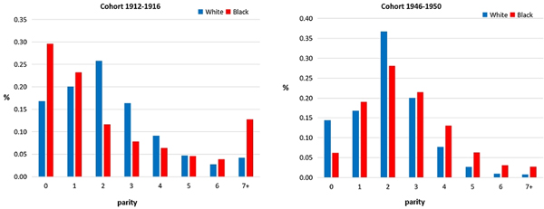
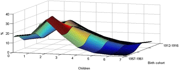
The TFR in the USA was decreasing at the beginning of the 19th century (Figure 1). At the beginning of 1800s, the TFR was approximately seven children (for white women—the rate was higher for black women). The TFR was approximately two children at the beginning of the second quarter of the 20th century (Figure 2). After a brief period of increase (the “Baby Boom”), the TFR returned to roughly two children (the “Baby Bust”), and remained relatively constant for the last 30 years of the 20th century. The periods of interest for this study are the 1930s and the 1970s, during which time the TFR was approximately two children. For these periods, consider another indicator of fertility behavior: the distribution of women by number of children (completed fertilities). Figure 4 depicts the distribution of women by number of children ever born for US women aged 45–49, born in 1912–1916 and 1946–1950, obtained from the National Vital Statistics System (NVSS). Despite the similarity of the average fertility (proxied by TFR) for these cohorts, their fertility behavior (fertility stopping rules) differed significantly. In the earlier cohort, some 60% of women had 1–3 children, less than a quarter of women had exactly two children, and roughly 20% of women had more than four children, making the average fertility a weak predictor of the completed fertility for any given mother. Women of the later cohort were more homogeneous in their fertility behavior. Almost 70% of women had 1–3 children, more than 35% had exactly two children, and large families became much more rare. However, the proportion of childless women, as well as women who had just one child in their lifetime, also decreased. Overall, the standard deviation of completed fertility decreased from 1.9 to 1.4, resulting in a distribution more concentrated around two children. A more complete picture of this concentration around two children (with multiple cohorts of women born between 1912 and 1961) can be observed in Figure 7. Note that in Figure 4 (as well as Figure 7), the distribution is presented for all women, while the analytical derivations (section 4) and numerical exercise (section 5) are performed for married women only. This raises concerns that some features observed in Figure 4 may be related to changes in celibacy rates, and that data on married women would be more appropriate for the purpose of this study. These data are available and are presented in studies such as Jones and Tertilt (Reference Jones and Tertilt2008). This study is interested in marital fertility and presents the distribution of married women (aged 40–45) by parity, obtained from the US Census data. The cohorts from 1908 and 1948 in Jones and Tertilt (Reference Jones and Tertilt2008), seen in their Figure A3, correspond most closely to those from NVSS that I use in my study. Changes in the distribution of fertility depicted in their Figure A3 are similar to the changes depicted in Figure 4 of my study; namely, we both observe a reduction in variability, as well as a reduction in the proportions of women with extreme parities (no children, one child, and three or more children) for the later cohort. Despite the availability of data on marital fertility, I decided to use NVSS data due to imperfections observed in the pre-1950 US Census data on childlessness. Namely, Baudin et al. (Reference Baudin, de la Croix and Gobbi2015) mention issues (relating to the classification of having no children) with the pre-1950 US Census data, which can potentially cause overestimation of childlessness rates. These issues are not present in NVSS, and the methodology of calculating the proportion of childless women is differentFootnote 1. Concerning changes in celibacy rates, Figure 7 in Fitch and Ruggles (Reference Fitch and Ruggles2000), using Current Population Survey (CPS), presents data on never married women. They show that between 1960 and 1995, among women aged 45–54, there was approximately a 1 percentage point decrease in the proportion of unmarried white women, although black women saw a 6 percentage point increase. Given that the black population was roughly 12% of the total population, the weighted effect implies that, for the total female population, the proportion of unmarried women was lower in 1995 compared to 1960. Due to this, I think that the change in marriage pattern cannot comprehensively explain the observed dynamics of childlessness and single-child women (although it undeniably had some effect). Fortunately, the data coming from NVSS has distribution by race, so I was able to obtain the likes of Figure 4 for each race separately (Figure 3) and it can be seen that the dynamics observed in Figure 4 are still present. In fact, despite the fact that there was an increase in the proportion of unmarried black women between 1960 and 1995, they experience a much more drastic decrease in childlessness than white women.
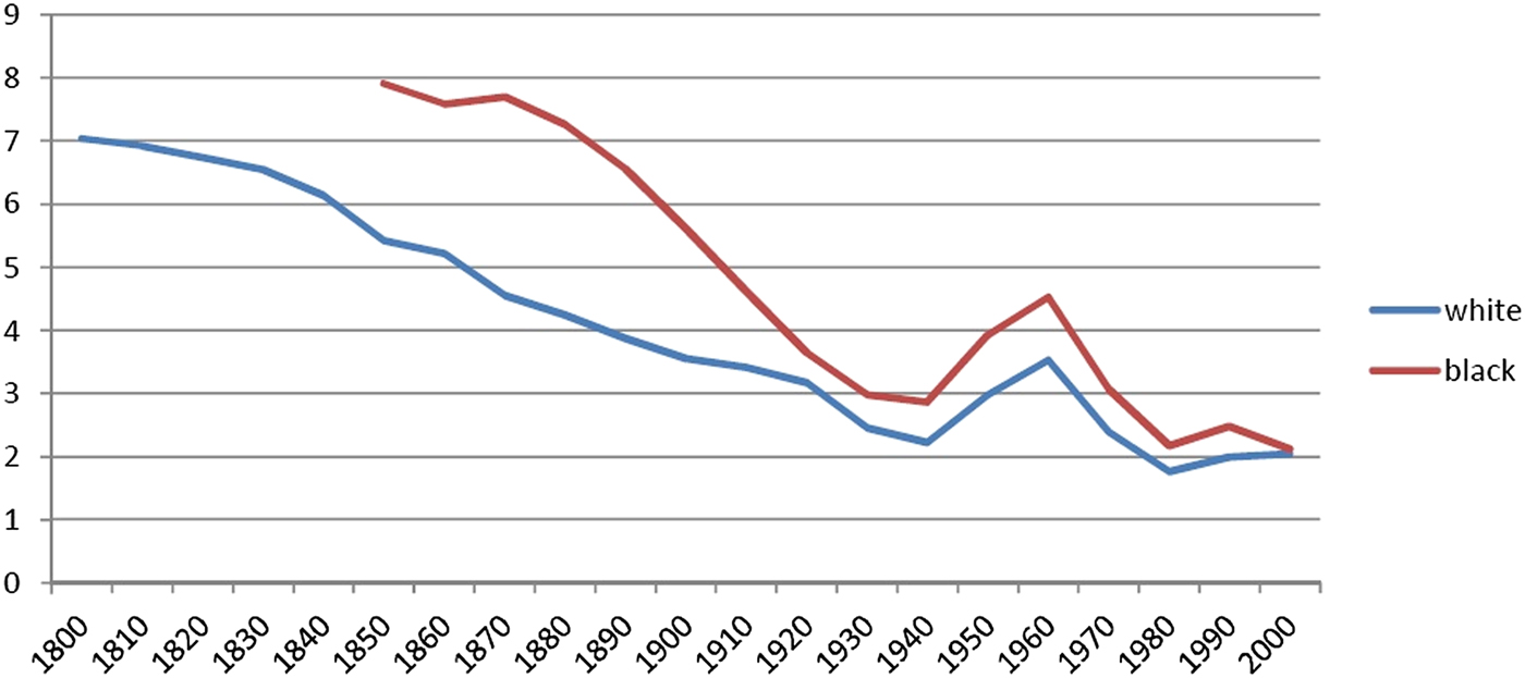
Figure 1. TFR, USA from 1800 to 2000 for White and Black women.
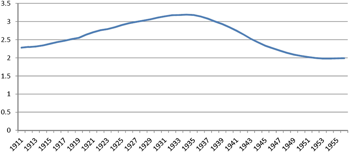
Figure 2. Average fertility of women aged 50, US birth cohorts from 1911 to 1955, all races.

Figure 3. Distribution of women by number of children ever born, US women aged 45–49 by races (White and Black), born in 1912–1916 and 1946–1950.

Figure 4. Distribution of women by number of children ever born, US women aged 45–49 of all races born in 1912–1916 and 1946–1950.
Another potential explanation for this childlessness may be the Great Depression. However, Sobotka et al. (Reference Sobotka, Skirbekk and Philipov2011) found that, during the Great Depression, the secular downward trend in fertility observed for the previous 100 years did not show significant signs of acceleration. This implies that the Great Depression did not necessarily have a major effect on completed fertility (as opposed to period fertility, which may change due to postponement). In fact, both of my cohorts of interest, those having children in the 1930s and the 1970s, were having children during a depression/recession (the mid-1970s saw a significant recession in the USA too, although not as harsh as the Great Depression). I would also suggest that one be careful to distinguish between the postponement of childbearing due to unfavorable economic conditions (although some may argue that a drop in wages could imply a reduced opportunity cost of having children) compared to the decision to have fewer children (completed fertility). The postponement of childbearing may have an effect on completed fertility if women tend to have children until they are no longer able to do so (natural limit). Because of this, it is obvious that postponement leaves fewer years until menopause, so fewer children can be born as a result. However, even for cohorts born in the 1850s, as evident from Jones and Tertilt (Reference Jones and Tertilt2008), such high fertility was very rare. Thus, if the households wanted to have six to eight children (which is a TFR observed in the early 1800s), postponing childbearing by several years should not significantly affect completed fertility.
Concerning the decrease in the proportion of women with many children, it is possible that some part of the decrease in the right tail may result from more efficient fertility control methods. However, note that even households which stopped at seven to eight children, let alone those which stopped at three to four, were, by no means, were close to the natural limit of fertilityFootnote 2. So, I assume that even households with highest parities households were able, somehow, to control fertility. Bailey and Hershbein (Reference Bailey and Hershbein2018) nicely summarize the argument on the control of fertility, noting that the drop in fertility started with women born in the 1850s and continued until the cohort in the 1910s. Moreover, that decline is explained, not by the change in the age of first marriage, but rather by the delaying and spacing of births, which implies significant control over fertility. Overall fertility now is not much lower than it was for the 1910s cohort, during which time “the pill” obviously did not exist. Thus, it is not obvious that earlier cohorts were unable to control fertility, or that fertility control was not very widespread. Note also that the proportion of childless and single-child households, as shown in Figure 4, was higher for earlier cohorts, implying that a significant part of the population was able to limit its fertility.
2.2 Empirical evidence of son-preferring differential stopping behavior
Childbearing, by nature, is a consecutive decision-making process. There is some evidence that the decision to have another child depends on the gender of the existing children in the household. In particular, the US households which had boy(s) at a lower parity (first, second, third child) were much less likely to have another child. For example, McDougall et al. (Reference McDougall, DeWit and Ebanks1999) cites a number of 1970s US studies that show that boys were preferred as a first or only child, and having more boys in the family was also preferred.
Dahl and Moretti (Reference Dahl and Moretti2008) conducted a more thorough empirical study of the probability of progression to another child, conditional on having girls vs. having boys. They used 1940–2000 US Censuses and found that households whose first two, three, or four children are girls have a higher probability of having another child compared to those with two, three, or four boys (the gender effect). The gender effect was stronger for women aged 20–30 born in the 1950s than for those born in the 1970s. However, women born earlier than the 1940s seemed to have a weaker gender effect. Note that they only report the effect in the case of two girls vs. two boys. A potential explanation for the weaker gender effect in the earlier cohorts may lie in the fact that earlier cohorts tended to have more children on average. No matter what, if a household wants to have three children, on average, one should expect a weak gender effect for the first two children. This idea is supported in Dahl and Moretti (Reference Dahl and Moretti2008) by the fact that, in developing countries, where average fertility is much higher than in the USA, the gender effect gets stronger at higher parities. To get a better picture over time, ideally one may need to have longer time-span data to identify women born in the early 20th century. However, the only data available for the USA that goes back in time to that extent is the Census and it unfortunately only reports children residing with their families. If one chooses women over the age of 40 with a hope of including only those who are close to finishing their fertility cycle, there is a risk that some children left the household.
The CPS fertility supplement can be used to cope with this problem. Supplements do not have a complete fertility record, as they report gender of only the first four children and the last child. However, as shown in Rosenblum (Reference Rosenblum2013) the gender of the first child (in the absence of gender-selective abortions practiced at the first birth) can be used to test for the presence of the SP-DSB). I use CPS fertility supplements for 1990 and 1995 obtained from IPUMS CPS, King et al. (Reference King, Ruggles, Alexander, Flood, Genadek, Schroeder, Trampe and Vick2010). In these supplements, fertility information is recorded only for those who were below the age of 66. Thus, from 1990, I select women who are married, aged 60–65, who had obviously finished childbearing, and have at least one child. From the 1995 sample, I choose married woman who are between 45 and 50 years old. Additionally, to ensure that they have finished childbearing, I choose those who stated that they did not intend to have additional children. Thus, the first cohort of women was having children in the mid-1940s and the mid-1950s, while the second cohort was having children in the 1970s. Having married women is important as the dissolution of marriage or loss of a spouse can potentially alter childbearing plans of a woman for a variety of reasons (like the cultural stigma of having children out of wedlock, or the deterioration of their financial situation due to staying single, etc.).
The following equation tests the presence of the son-preferring fertility stopping rule:
 $$y_i = \alpha + \gamma X_i + \theta t + \tau Z_i + \varrho Z_i\cdot t_i + u_i,$$
using the pooled data of CPS 1990 and 1995, where y i is the number of live births, X i is a vector of variables, which includes race, age at first birth, labor market status of a women, female labor force participation rate in the state of residence, and her education levelFootnote 3; t i is an indicator (dummy) variable for women of the younger cohort (women from the CPS 1995 sample aged 45–50), Z i is an indicator variable of a first-born male child and Z i · t i is an interaction term. Results of the regression (1) are shown in Table 1. It is clear that women of the earlier cohort had fewer children if the first child was a boy. The Ordinary Least Squares (OLS) estimates (first column) indicate that women with a male first-born had approximately 0.2 fewer children. For comparison, Rosenblum (Reference Rosenblum2013) obtains 0.35 fewer children for India where son-preference is well-documented. Given that I count data where a count of 0 is impossible (I included women who had at least one child), I also estimate equation (1) using zero-truncated Poisson regression, which implies (second column) approximately 5 percentage points fewer children for those with first-born sons. This effect is statistically significant. Moreover, the effect of the first-born child's gender on the later cohort is negative too, but has a smaller magnitude. Other variables in X i have expected signs: higher age at first birth, being white, being in the labor force, and being more educated tend to reduce completed fertility. Interestingly, the education variables are highly non-significant, which might be explained by the fact that I control for age at first birth, which is likely connected to the level of education (the more a woman studies, the more likely she will have a child later in life). Indeed, if one omits the woman's age at the first birth, the education variables become significant. Labor force participation at the state level reduces the effect of the first-born's gender, but only marginally, and itself is highly non-significant, a result probably stemming from the issues discussed above. Being limited to only 1990 and 1995, the data allow me to go back no further than the 1925–1930 cohort, which is some 15–20 years later than the earlier cohort in Figure 4. Even this is enough to see that the smaller gender effect for the pre-1940s cohorts in Dahl and Moretti (Reference Dahl and Moretti2008) can be due to the problems with the data discussed above. In summary, there is empirical evidence that early cohorts of US households exhibited son-preferring fertility stopping behavior. For the later cohorts, there is weak, if any, evidence for such fertility behavior.
Table 1. Estimation of gender stipulated fertility stopping behavior

Notes: The sample consist of married women who had at least one live birth and at the moment of the survey has completed fertility (testified by being in the age of menopause as well as directly stating absence of intention to have more children). Independent variable is the number of live births a women ever had. Data come from CPS Fertility Supplements 1990 and 1995 (obtained from IPUMS-CPS). OLS uses final basic weights. For zero-truncated Poisson e τ is the average ratio of number of children of women with male first born to the number of children of a women with female first born. ***significant at less than 1%; **significant at 5%; *significant at 10%.
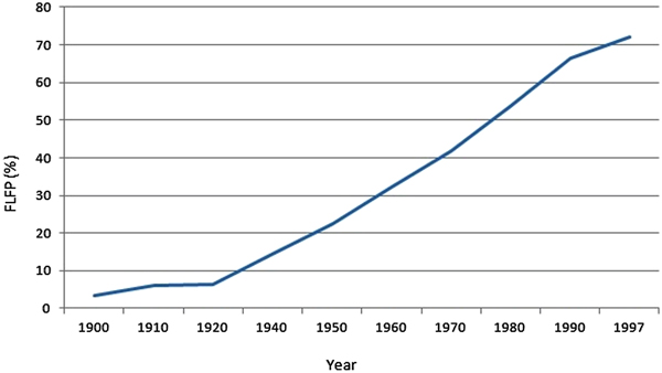
2.3 Evolution of the labor force participation of the married women over time
The 20th century also saw significant changes in the composition of the workforce in the USA (Figure 5) and other developed nations. An important phenomenon was the emergence of married working women. Women were employed in the formal labor market throughout 19th century in quite large numbers, but these were mostly unmarried women. After marriage, most of these employed women tended to leave labor market. However, from the early 20th century onward, that trend started to change. As shown in Figure 5, the proportion of married women in the labor force (FLFPR) constantly rose during all of the 20th century. If less than 5% of married women in the 1900s were in the labor force, by the 1990s, this number rose to approximately 70%.

Figure 5. Percentage of married women in labor force.
The choice of the FLFPR as a factor affecting parental choice is not random. Mills and Begall (Reference Mills and Begall2010), in their study of gender preference in Europe, come to the conclusion that, in places where there is a lower gender equity, clear preference for sons exists. I think it is not unreasonable to use the FLFPR as a metric of gender equity, ultimately affecting child gender preferences. After all, the presence of women in leading positions in business, politics, academia, sports, military, etc. is perceived as a sign of gender equality, making women socially and economically indistinguishable from men. Another often-cited measure of equality between sexes is the gender gap in wages. However, the precondition for the existence of a gender gap is the existence of employed women. The FLFPR of married women was steadily increasing and I believe this captures the changes in gender roles and movement toward gender equality that occurred over the past century. In this context, I see the FLFPR as a reasonable proxy for the advances in the status of women in society, which should positively affect parental satisfaction from children, whether we view parents as altruistic or egoistic. From an altruistic point of view, being in the labor market and having one's own income source may mean more freedom in choosing a partner (the choice is not limited to those who can “provide”); higher bargaining power within a family (a financially independent female's value of outside (to marriage) option is higher in the case of divorce); potential well-being of grandchildren (e.g., working daughters would not appear in sharp poverty in case of the death of the husband), and, of course, the pride of the daughters’ self-realization in the professional domain. For egoistic parents, working daughters may mean a higher chance of receiving old-age support, either because daughter's family will have more income to share, or due to the above-mentioned stronger bargaining position to insist on supporting her parents. Note that many of the factors favoring daughters in the labor force are linked to a notion of girls becoming good mothers (ability to avoid poverty in the very common case of early death of a husband, education to help their own children with schooling, etc.). So, even in a society where the middle class may maintain “patriarchal views” on the role of women, working should not be viewed as incompatible with that role. After all, even in rural communities, which usually tend to be more patriarchal, women from early ages are expected to work both at home and on the farm.
3. The model
3.1 Modeling approach
Given that women's status in society is proxied by the likelihood of being in the labor force as a married woman, it seems natural to model parental preferences such that they derive utility from the income of their children. In such an approach, the parental utility from children would be dependent on the expected labor market status of their children. Fortunately, modeling parental preferences, such that they derive utility from the income of children, is quite common in the literature, e.g., Galor and Weill (Reference Galor and Weill2000), de la Croix and Doepke (Reference de la Croix and Doepke2003), Kalemli-Ozcan (Reference Kalemli-Ozcan2003), and Hazan and Zoabi (Reference Hazan and Zoabi2015). Note, however, that by total income of children, I do not mean a discounted lifetime income earned by children (too complex to model, as discussed below), but rather the sum of wages of all children earned per unit of time, where these wages depend on the amount of human capital. In this sense, these wages, which can be earned per unit of time due to the presence of a child in the labor market, demonstrate the child's “earning potential.” One may also say that a child's income (per unit of time) is a measure of indirect utility, as the child's “earning potential” captures the tightness of the budget constraint to be faced to the future.
3.2 Model setup
The society consists of a single cohort of an arbitrary large number of households, which are ex-ante identical (the same age, income “earning potential”, preferences, budget constraints, etc.)Footnote 4. A household consists of a male and a female who jointly behave as one economic agent, and make decisions on having children and investment in the human capital formation of children. Each household has four uncertainties affecting its decision: (1) uncertainty over the labor force status of its female: each household has the equal probability α (that is the current FLFPR) of the female of the household participating in the labor market; (2) uncertainty over its level/valuation of “outside” option to childbearing ξ j; (3) the gender of each consecutive child (once they start childbearing); and (4) the labor force status of their daughters (if any): probability of being employed is proxied by the current FLFPR (α). The first two uncertainties are realized at the onset of the childbearing decision, i.e., the household learns the labor force status of its female and its level of “outside” option and only then starts to plan childbearing. The third uncertainty is resolved at childbirth, and the forth uncertainty is resolved only when the children grow up, that is when all household decisions concerning human capital investment and fertility progression have been made.
I study the effects of the increased FLFPRFootnote 5 on the example of a fertility model whose variation can be found in Galor and Weill (Reference Galor and Weill2000), de la Croix and Doepke (Reference de la Croix and Doepke2003), Kalemli-Ozcan (Reference Kalemli-Ozcan2003), Hazan and Zoabi (Reference Hazan and Zoabi2015), etc. It is a one-time model where households, observing the exogenously given FLFPR, determine whether or not to have children, and if they decide to have children, when to stop having them. A household derives utility from their own consumption and from the expected income of its children if it has child(ren), or from the level of “outside” options available to it, if it chooses not to have any child. This means that parents, who have children, derive utility only from children who will be employed. This statement requires clarification. Altruistic parents enjoy children even if they are not employed. Thus, in the initial version of the study, parents derived utility from the total income of children who were expected to work, and children not in the labor market contributed some constant χ to the parental utility. That χ was to stand for the “pure joy” or “intrinsic happiness” of having a child regardless of its labor market status. However, this addition made analytical derivation difficult. Assuming that there is no reason why this “pure joy” of having offspring should be different between sexes, I “normalized” χ to zero. This simplification comes with the additional benefit of making the FLFPR similar to child survivability, thus allowing the use of theoretical results obtained in studies such as Sah (Reference Sah1991) and Kalmli-Ozcan (2005). For further discussion on the effect of the choice of the utility function on the main results of this study, please refer to Appendixes A-10 and A-11, where numerical estimation using several more general utility function specifications yield similar fertility stopping rules.
In the simplified model, all boys are assumed to become employed adultsFootnote 6. Each of the girl's probability of being employed is given by the current FLFPR (in this model, it is the best estimate of that probability in the future). As all girls have the same probability of being an employed woman, the expected number of employed girls is characterized by a binomial distribution. As a result, the household's expected utility functionFootnote 7 is
 $$\left\{ {\matrix{ {U_j\,(c,e_b,e_g,b,g) = u\,(c) + \psi \mathop \sum \limits_{i = 0}^g \alpha^i\left( {\matrix{ g \cr i \cr}} \right)\,{(1-\alpha )}^{g-1}v\,(bh_bw + ih_gw),\,{\rm if}\,b \gt 0\,{\rm and/or}\,g \gt 0} \cr {\,\,\,\,\,\,\,\,\,\,\,\,\,\,\,\,U_j(c,e_b,e_g,b,g) = u\,(c) + \psi v\,(\xi_j),\,{\rm if}\,b = 0\,\,{\rm and}\,\,g = 0,} \cr}} \right.$$
where u (.) and v (.) are two differentiable concave functions. The c is the lifetime consumption, b is the number of boys in the household, each of whom gets e b of household resources invested in human capital formation, g is number of girls in the household, each of whom gets e g of household resources invested in human capital formation. I make a simplification that all households are fertile. In this case, a household stays (voluntarily) childless if the “outside” option to being parentsFootnote 8, which I denote by ξ j, delivers more utility to the household j than having a child (described in detail in the next subsection). If households decide to have a child, then parents are obviously “inside” parenting and do not derive utility from an “outside” option ξ j. The ψ is the level of parental altruism. A child's human capital is denoted by h k, k = {b, g} and the human capital formation function is  $h_k = e_k^\gamma $, where k = {b , g}, 0 < γ < 1 and the (per unit of time) wage per unit of human capital is w. The FLFPR is the probability of a girl becoming an employed women and is denoted by α. Note that, when households start developing their contingency plan (fertility stopping rules), they face uncertainties (3) and (4). This last source of uncertainty is incorporated in the expected utility function similar to the incorporation of child survivability in studies like Sah (Reference Sah1991), Portner (Reference Portner2001), and Kalemli-Ozcan (Reference Kalemli-Ozcan2003). Thus, the utility function used in this study is a combination of a utility function that has uncertainty over child gender and a utility function that has uncertainty over the “survivability” of the children. The budget constraint is
 $$\matrix{ {c + be_b + ge_g = y_m-p(b + g) + y_f\,(1-z\,(b + g)),\,y_f = \lsqb {0,{\overline y}_f} \rsqb } \cr}. $$
 The male and female of the household are each endowed with a unit of time, which can earn income y m for the male and income  $y_f = \overline y _f$ for the female, if she is in the labor market and y f = 0 if she is not part of the labor forceFootnote 9. If the female of the household is part of the labor force, then the household is considered to be of type I, otherwise it is considered to be of type II. I assume that females specialize in raising children, so the time opportunity cost z is incurred only by them. The p ∈ (0, 1) is the fixed cost of having a child in terms of goods. The presence of p (and z) is crucial, otherwise households can continue having children until they get the required number of boys, and a household with, for example, three boys will be equivalent to a household with three boys and any number of girls. I assume that, like the cost of having a child (p), the cost of education is also in terms of consumption goods. However, the nature of costs of child-bearing and education does not play any significant role in this model as α does not enter u(.), so the results hold if any of these costs, or both, are in terms of parental time or consumption goodsFootnote 10.
3.3 Description of the household's problem
After uncertainties (1) and (2) are resolved, households proceed to plan for childbearing, which is done following a two-stage maximization procedure.
In the first stage, for any number of boys and girls (b, g), a household determines how much investment will be made into the human capital of each boy and each girl (determination of e b and e g). This is done by maximizing utility (2) subject to constraint (3) for each possible pair of (b, g). In the second stage, given the human capital investment plan at every possible gender outcome of each consecutive pregnancy, the household develops a fertility stopping rule. At any possible pair (b, g)Footnote 11, if the household decides to have a child, with equal probability, it will have (b + 1, g) or (b, g + 1) children. Let V (b, g) stand for maximized utility for a given (b, g), while V (b + 1, g) and V(b, g + 1) be maximized utilities for (b + 1, g) or (b, g + 1) children. The household will find it optimal to have another child only if the expected utility from having another child is greater than staying with current number of children (b, g); that is MU(b, g)—marginal utility from having another child (4) at parity (b, g) must be positive. Thus, the household can determine whether it will continue childbearing at every physically conceivable parity (b, g). So, at the moment the household starts having children, it already has the complete plan of action regarding educational and fertility choices—the fertility stopping rule:
 $$MU(b,g) = 0.5V(b + 1,g) + 0.5V(b,g + 1)-V(b,g).$$
 In essence, households develop a contingency plan, before starting childbearing, but after the resolution of uncertainties (1) and (2). Think of that contingency plan as an action tree. At the beginning, a household with no children knows that the first child will be a boy or a girl with equal probability. It can determine the optimal investment in human capital in case the child is a boy, and in case it is a girl. If the expected utility from having a child outweighs the utility of staying childless (“outside” option) the household will have the first child. Note that, for a given level of the FLFPR (α) and the labor status of the female in the household (type I or type II), there are two threshold levels  $\tilde{\xi} _I^\alpha $ and
  $\tilde{\xi} _{II}^\alpha $ of constant ξ j, above which households do not have children. The assumption that ξ j is irrelevant for those who have already started childbearing avoids increased complexity due to a new dimension of heterogeneity. So all type-I households, who started childbearing, are identical (thus, they have the same contingency tree), and the only thing distinguishing them is the fertility history that they will have. The same is true for type-II households. This simple assumption allows the model to generate childlessness and avoid any external factor (except the FLFPR), changing the contingency tree. After having the first child, the household continues as described above: for a given node (b, g) on the contingency tree, it determines the optimal education investment for the (b + 1, g) and (b, g + 1) nodes and determines whether to proceed with an additional child based on the sign of the marginal utility (4). The node at which the household stops childbearing will totally depend on its fertility history, i.e., the series of random resolutions of gender uncertainty (3). Thus, the complete contingency plan for type-I and type-II households is a tree with branches of various lengths. Given the contingency trees, it is clear that, as a result of childbearing, the initially identical mass of type-I and type-II households will be distributed over the nodes of trees generating fertility variation. The main task of this study is to see how trees for type-I and type-II households change when the households appear in environments with a different FLFPR.
3.4 Son-preferring differential stopping behavior (SP-DSB)
The fact that, at a FLFPR<1, not all girls may end up being employed women implies that households, whose first-born children are girls, will tend to have another child in the hopes that it will be a boy. To see this in a simple setup, assume an exogenous human capital case where each child is born with a unit of human capital earning w = 1. Assume also a household A, which has (b + 1, g) children, and a household B, which has (b, g + 1) children. For the simplicity of this exposition, I assume that both households are of type II (actually, as long as households A and B are of the same type, the exact type does not matter). The marginal utilities from having another child for these households (household type is denoted by subscript) at an extremely low FLFPR (I consider the case of α = 0) areFootnote 12
 $$\eqalign{MU_A\,(b + 1,g) &= u\,(y_m-(b + g + 2)p)-u\,(y_m-(b + g + 1)p) + 0.5\psi \,(v(b + 2) \cr &\quad -v(b + 1)),}$$
 $$\eqalign{MU_B\,(b,g + 1) &= u\,(y_m-(b + g + 2)p)-u\,(y_m-(b + g + 1)p) + 0.5\psi (v(b + 1) \cr &-v(b)).}$$
As MU A (b + 1, g) <MU B (b, g + 1)Footnote 13, even in the case of MU A (b + 1, g) = 0 (utility maximizing fertility achieved), household B will have another child as MU B(b, g + 1) > 0, so household B will exhibit SP-DSB. Thus, even if we have ex-ante identical households, at low FLFPR levels, households A and B will end up with different levels of completed fertility simply because, at a low FLFPR, they will exhibit SP-DSB and child gender determination is a stochastic process.
4. Effect of FLFPR on the decision making of households
In this section, I study the effect of changing the FLFPR on household decision making. First, I show how changes in the FLFPR affect fertility decisions of the voluntarily childless households. Then, I move to the general setup and present the effects of changing the FLFPR on the first (education) and the second (fertility) steps of the household utility maximization problem. As the fertility reaction to a changed FLFPR in the general case is ambiguous, subsections 4.5 and 4.6 study the household optimization problem in special cases: a household that has only boys and a household that has only girls. The effect of the FLFPR on household decision making in these special cases allows the understanding of what happened to the tails of the distribution of women by number of children observed in Figure 4. Most of the results are obtained assuming a generic budget constraint (3). The labor status of a female does not qualitatively affect the results. That status will affect results quantitatively; this is studied in the numerical exercise in section 5.
4.1 Marginal households
Before studying the effect of changes in the FLFPR, I need to define the Marginal Households. I will be studying the effect of changes in the FLFPR on the behavior of these households. The Marginal Household MH (b, g, α 0) is a household, which at a given number of children (b, g)Footnote 14 and FLFPR (α 0), is indifferent to having another child or abstaining from having one that is, the marginal utility of having another child (5) is zero.
4.2 Childless households
I start the study of household behavior with households which, at lower FLFPR, decide to stay childless. Unlike the general case of a household which has b > 0 boys and g > 0 girls, in this simple case, the effect of the FLFPR on education and the fertility decision is mathematically tractableFootnote 15.
A household chooses to have the first child if having that child delivers more utility than the “outside” option of choosing to stay childless, ξ j (MU (5) is positive).
 $$\eqalign{MU &= 0.5\,(u(y_m-p-e_b-y_f\,(1-z)) + v\,(e_b^\gamma ) \cr & \quad + 0.5\,(u(y_m-p-e_g-y_f)\,(1-z)) + \alpha v(e_g^\gamma )) \cr & \quad -u(y_m + y_f)-v\,(\xi _j).} $$
Proposition 1. In an environment with α 1 such that α 1 > α 0 the MH (0, 0, α 0) will definitely have another child as MU (5), for a given ξ j, will be positive.
Proof: See Appendix A-1.
This result is similar to the “essential complementarity” discussed in Aaronson, Lange, and Mazumder (Reference Aaronson, Lange and Mazumder2014). To gain from an increased FLFPR, parents must have at least one child. Note that Proposition 1 implies that the threshold for the level of “outside” options at which households prefer to stay childless should be higher at α 1, i.e.,  $\tilde{\xi} _j^{\alpha _1} \gt \tilde{\xi} _j^{\alpha _0} $. Thus, a higher FLFPR implies a smaller proportion of households staying childless. This result is consistent with the situation observed in Figure 4, where the later cohort contains 5 percentage points fewer childless women than the earlier cohort.
4.3 Change in the education decision for a household with an arbitrary number of boys and girls
Starting from this subsection, to facilitate analytical derivations, all results are obtained assuming logarithmic u (.) and v (.) functions.
Let us take a household with an arbitrary number of boys and girls (b, g)Footnote 16.
Substituting
 $$c = y_m-(b + g)\,p-be_b-ge_g-y_f\,(1-z\,(b + g))$$
and
 $$E\lsqb {v\,(e_b,e_g,b,g)} \rsqb = gi = 0\mathop \sum \nolimits \alpha ^i\left( {\matrix{ g \cr i \cr}} \right)\,(1-\alpha )^{g-i}v\,(be_b^\gamma w + ie_g^\gamma w),$$
into utility function (2) the First Order Conditions (FOCs) for investments in human capital are:
 $$e_g{\kern 1pt} :\,\,u_{e_g}\,(e_b,e_g,b,g) + E\lsqb {v_{e_g}\,(e_b,e_g,b,g)} \rsqb = 0$$
 $$e_b{\kern 1pt} :\,\,u_{e_b}\,(e_b,e_g,b,g) + E\lsqb {v_{e_b}(e_b,e_gb,g)} \rsqb = 0.$$
To know how the investment in human capital changes when the FLFPR changes, I take the full derivative of FOCs (6) and (7) with respect to α which allows the establishment of the following proposition:
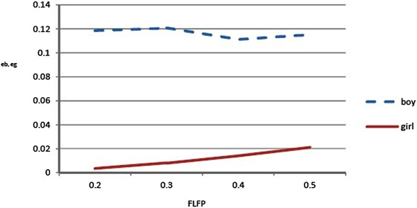
Proposition 2. For a given number of boys and girls (b, g), ∂e b/∂α < 0 and ∂e g/∂α > 0.
Proof: See Appendix A-2.
Within a household, an increase in the FLFPR makes parents relocate some of their resources from boys to girls. The intuition is simple: the human capital function is concave. At a higher FLFPR, an investment in girls becomes less risky, the expected marginal return from education increases, so an investment in girls becomes more attractive. Obviously, when the FLFPR is 1, boys and girls are identical “assets” and all children, regardless of gender, will receive the same education. The same result is obtained numerically for relatively concave utility functions.
4.4 Change in the fertility decision: the “stock” and “flow” effects
The effect of changing the FLFPR on the investment in human capital of boys and girls is not hard to predict. In the extreme case of the FLFPR being 0, it is clear that no investment is made into the human capital of girls, while when the FLFPR is 1, boys and girls, being identical, are treated equally. The previous section helped determine the trajectories at which investments in human capital for boys and girls will converge when the FLFPR increases.
To study the effect of an increased FLFPR on the decision to have another child, assume that at an arbitrary α = α 0 there is a MH (b, g, α 0). My goal is to see whether this marginal household (which is indifferent to having another child, or not, at the current α 0) definitely will or will not have another child in case it appears in an environment with α = α 1, such that α 1 > α 0. To do this, I totally differentiate MU (4) with respect to α. Obviously, if the derivative of the marginal utility with respect to α (MU α) is positive, the household will have an additional child, as the marginal utility from having another child becomes a positive number. If it is negative, the household will abstain from having another child, as the marginal utility from having another child becomes a negative number. As V(b + 1, g), V(b, g + 1), and V(b, g) are all utilities maximized by the optimal level of investment in human capital of boys and girls, the Envelope Theorem states that the change in marginal utility is equal to the direct effect of the FLFPR on the marginal utility function, which is the following expression (8):
 $$\eqalign{MU_\alpha &= 0.5\,(\partial E\,[v\,(e_b(b + 1,\,g,\,\alpha _0),\,e_g(b + 1,\,g,\,\alpha _0),\,b + 1,\,g)]/\partial \alpha ) \cr & \quad -0.5\,(\partial E\,[v\,(e_b(b,\,g,\,\alpha _0),\,e_g(b,\,g,\,\alpha _0),\,b,\,g)]/\partial \alpha ) \cr & \quad + 0.5(\partial E\,[v\,(e\,(b,\,g + 1,\,\alpha _0),\,e_g(b,\,g + 1,\,\alpha _0),\,b,\,g + 1)]/\partial \alpha ) \cr & \quad -0.5(\partial E\,[v\,(e(b,\,g,\,\alpha _0),\,e_g(b,\,g,\,\alpha _0),\,b,\,g)]/\partial \alpha ) \lessgtr 0,} $$
where e b(b + 1, g, α 0), e g (b + 1, g, α 0), e b(b, g + 1, α 0), e g(b, g + 1, α 0), e b (b, g, α 0), and e g(b, g, α 0) are optimal levels of investment in human capital for a household with (b + 1, g), (b, g + 1), and (b, g) children at α = α 0 (see Appendix A-3 for details of expression (8)). Unfortunately the sign of expression (8) is hard to identify. One may think that different levels of education are behind the ambiguity of expression (8). However, even in case of exogenous human capital (see Appendix A-4), the sign of expression (8) remains ambiguous.
I identify two effects which can intuitively explain why we have ambiguous results. These effects are themselves a complex interaction of certain phenomena, and I can separate these effects based on the different directions in which they move the MU α. Intuitively, I call them the “flow” and “stock” effects. Increasing the FLFPR makes the expected “flow” of utility from an additional child bigger, so I call this the “flow effect.” On the other hand, if the household already has girls, a change in the FLFPR will affect each girl, increasing the expected “stock” of utility from the existing “portfolio” of children, so I call this the “stock effect.” Note that the “stock effect” is bigger when a household has more girls. Both the “flow” and the “stock” effects, generated by increases in the FLFPR, tend to increase utility, but their interplay, which determines the effect on marginal utility, is more complex. This is why I propose to consider two polar cases in which only one of the effects will be present to see in which direction they move the MU. Below, I present the case of a household which has only boys, and the case of a household which has only girls.
4.5 Case 1: A household with only boys
To start, assume there is a household that has b boys, that is considering having another child. In case that they know the child is a boy, the marginal utility from that child does not depend on the FLFPR. Thus, changes in the FLFPR have no effect on the decision of whether or not to have another child. The “flow” effect is illustrated when this household knows that the next child will be a girl, as changes in the FLFPR affect only that girl. In that case, the marginal utility from that additional girl is expression (9):
 $$MU = V(b,1)-V(b,0).$$
Intermediate result 1. In an environment with a higher FLFPR, a household with b boys has greater incentive to have another child.
Proof: Appendix A-5.
This is due to MU α>0. As the existing “stock” of children is not affected, only the expected gain from an additional child increases, while the marginal cost of having that child stays the same. This is what we have referred to as the “flow effect.” The same result holds true for the case of exogenous human capital of children (Appendix A-6), indicating that education is not the main driving force behind this result.
What if the gender of the next child is unknown? As described in subsection 4.4, the marginal utility from another child whose gender is unknown is just an average of marginal utilities from having a boy and a girl (10):
 $$0.5\,(V(b + 1,0)-V(b,0)) + 0.5\,(V(b,1)-V(b,0)).$$
Proposition 3. In an environment with α 1 such that α 1 > α 0 the MH (b, 0, α 0) will definitely have another child as the MU (10) will be positive.
Proof. The additive nature of the MU (10) allows us to look at the MU α as a sum of derivatives of the marginal utility from Intermediate result 1 and MU of a household whose next child is surely a boy. In an environment with a higher FLFPR, the MU (10) of the MH (b, 0, α 0) will be a positive number at a higher FLFPR (α 1). This is due to the fact that the derivative of marginal utility from having a boy is zero and, from Intermediate result 1, the derivative of the marginal utility from having a girl is positive.
4.6 Case 2: A household with only girls
Another special case is when a household has g girls and considers having another child. Assume that it knows that the next child will be a boy. Here, only the “stock” effect is in play as changes in the FLFPR do not affect additional utility generated by this boy. The marginal utility from having a boy for this household is
 $$MU = V(1,g)-V(0,g).$$
Intermediate result 2. In an environment with a higher FLFPR, a household with g girls has less incentive to have the expected boy.
Proof: see Appendix A-7.
This is because the MU (11) is a decreasing function of the FLFPR (MU α < 0). It is tempting to think that once the FLFPR increases, the investment in human capital of girls becomes more valuable, so the household decides to abstain from having another child in order to invest more in each girl. However, this is not the case. Even in the case of exogenous human capital of children, this result holds, and parents abstain from having another child (see Appendix A-9). The observed phenomenon reflects the “prudence” of the household [see Leland (Reference Leland1968), for instance]. Increases in the FLFPR mean that both the expected return (from children) and the variance of that return change. This is due to the fact that, in the case of a binomial distribution of the return on assets (children), the FLFPR affects both the mean and the variance of that distribution. Due to the logarithmic utility function, income and substitution effects caused by an increased return cancel each other out, leaving only the effect of the changed variance, that is changed uncertainty. If the FLFPR is low, the household will engage in precautionary saving, i.e., it will have many children. As the uncertainty over the number of employed girls decreases with a higher FLFPR, the household reduces its precautionary demand for children.
The same “prudence” is at work in another case, when a household with g girls considers having another child and it is known to be a girl.
Intermediate result 3. In an environment with a higher FLFPR, a household with g girls has less incentive to have the expected girl.
Proof. Appendix A-8.
This is because the MU (11) is a decreasing function of the FLFPR (MU α < 0). Note that the model with exogenous human capital of children delivers the same resultFootnote 17. As previously mentioned, the FLFPR is employed in my model as child survivability/mortality is employed in many fertility models, which makes results comparable across models. More specifically, when an all-girl household knows that it will have a girl, my model is similar to the model developed by Kalemli-Ozcan (Reference Kalemli-Ozcan2003). Kalemli-Ozcan shows that the increase in the child survivability rate reduces the marginal utility from another child, implying a reduction in fertility, which is caused by a reduction in the precautionary demand for children. Similar also is a study by Portner (Reference Portner2001) where marginal utility (with no restriction on the form of the utility function) from another child is more likely to be decreasing in child survivability the more parents are risk averse and the more positive the third derivative of the utility function is (prudence). Additionally, Rosati (Reference Rosati1996) states that an increase in variance of the infant mortality rate increases the demand for children.
Now assume there is a household with g girls, which considers having another child, whose gender is ex-ante unknown. Given the stochastic nature of child gender determination, two states of the world are possible. In one, the next child is a boy and in another, it is a girl. Marginal utility from having that child is the expected utility from having a child (equal-weighted sum of the utilities in two states of the world) minus the current utility (12):
 $$MU = 0.5\,(V\,(1,g)-V\,(0,g)) + 0.5\,(V(0,g + 1)-V(0,g)).$$
Proposition 4. In an environment with α 1 such that α 1 > α 0 the MH (0, g, α 0) will definitely abstain from having another child as MU (12) will be negative.
Proof. The additive nature of the MU (12) allows us to look at the MU α as the sum of the derivatives of the marginal utility from Intermediate results 2 and 3. Intermediate result 2 states that, for those who have only girls and the next child is a boy, an increase in the FLFPR has a negative effect on the marginal utility. Intermediate result 3 states that if the next child is a girl, the change in marginal utility is also negative, so that the MU (12) of the MH (0, g, α 0) is negative for a higher FLFPR (α 1).
4.7 Changes in the distribution of women by number of children
The study of the all-boy and all-girl household polar cases in subsections 4.4 and 4.5 is important for us to understand the concentration of the distribution of women by number of children, as observed in Figure 4. As previously stated, low fertility households tended to be all-boy households, or ones where the first-born children were boys, while households with larger families tended to be all-girl households, or ones where girls were the first-born children. Thus, from Case 1 and Case 2, we can conclude that as the FLFPR increases, households on one extreme (few children) increase their fertility, while households on the other extreme (many children) decrease their fertility, so that the distribution becomes more concentrated.
It is reasonable to conjecture that households with children of both genders will resemble the behavior of households in Case 1 and Case 2 depending on the relative number of boys and girls in the household. This is an important feature of this study. The fertility stopping rules depend not only on the number of children, but also on the fertility history (gender mix of children) in the household. This is why MU α is ambiguous in subsection 4.3 for a general case of a household with b boys and g girls.
To verify the conjecture on the behavior of household with an arbitrary number of boys and girls, as well as to illustrate the evolution of the fertility stopping rules as the FLFPR increases, I conduct a numerical exercise. Note that the numerical exercise is not a calibration/simulation exercise (although parameter values are assumed so that resulting TFR resembles those observed in Figure 4), but rather a way to visualize fertility stopping rules and their evolution when the FLFPR increases. Thus, the parameters are chosen to capture the major features of Figure 4, rather than precisely replicating it (e.g., the model generates a higher proportion of single child households than observed in Figure 4).
5. Numerical exercise
5.1 Parameters
As described in section 3, before childbearing, households learn their type. In type-I households, the female is in the labor force, while in type-II households, the female is not in the labor force. The current FLFPR is the proportion of type-I households in society. Knowing their type, households observe the level of available “outside” options to being parents. The expected utility functions for households which decide to have children, that is whose levels of “outside” options to being parents are below threshold values of  $\tilde{\xi} _I^\alpha $ and
  $\tilde{\xi} _{II}^\alpha $, are (13) for type-I and (14) for type-II households:
 $$\eqalign{U_I &= u(y_m-(b + g)p-be_b-ge_g + y_f\,(1-z(b + g))) \cr & \quad + \psi \sum\limits_{i = 0}^g {\alpha ^i} \left( {\matrix{ g \cr i \cr}} \right)(1-\alpha )^{g-i}v\,(b(e_b)^\gamma w + i(e_g)^\gamma w)} $$
 $$\eqalign{U_{II} &= u((y-(b + g)p-be_b-ge_g)) \cr & \quad + \psi \sum\limits_{i = 0}^g {\alpha ^i} \left( {\matrix{ g \cr i \cr}} \right)\,(1-\alpha )^{g-i}\,v(b(e_b)^\gamma \,w + i + (e_g)^\gamma w).} $$
 The u(.) and v(.) functions are of the Constant Relative Risk Aversion (CRRA) type with a coefficient of relative risk aversion equal to 0.5. The y m and y f are male and female lifetime earnings. The cost of child p, investments in human capital e b and e g are all in terms of goods, which are paid from the total income of the household. In addition to the fixed cost of p, for type-I households, each child comes with an additional cost of z, which is a fraction of the female's lifetime income forgone due to having a child. Echevarria and Merlo (Reference Echevarria and Merlo1999) estimate that, in Canada, raising a child costs women 5% of their lifetime income, while in de la Croix and Doepke (Reference de la Croix and Doepke2003), the cost of a child is estimated to be 7.5% of their lifetime income. I stay close to these numbers and assume p = 0.05 (5%) and the rest is expenses on education. The opportunity cost of having a child is assumed to be z = 0.05 (5%), if we assume that a women works for 40 years, and with every child, she loses approximately 2 years of earnings. Lifetime earnings of a male are normalized to 1 and given that there was always a wage gender gap, female lifetime income is assumed to be 70% (y f) of male income. The γ of the human capital accumulation function is assumed to be 0.5 as in Hazan and Zoabi (Reference Hazan and Zoabi2015). The altruism parameter ψ is set equal to 0.25 to obtain an average fertility rate of approximately 2, which was the TFR observed in the 1930s when the FLFPR was approximately 0.2. The distribution of “outside” options ξ j is assumed to be log-normal with μ = −4.567 and σ = 2.643. These parameters are chosen such that the proportion of childless women at a FLFPR of 0.2 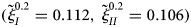 $(\tilde{\xi} _I^{0.2} = 0.112,\,\tilde{\xi} _{II}^{0.2} = 0.106)$ and 0.5
  $(\tilde{\xi} _I^{0.5} = 0.206,\,\tilde{\xi} _{II}^{0.5} = 0.188)$, which correspond to the values of the FLFPR observed during the reproductive lifetime of the cohorts from 1912–16 to 1946–50, are comparable with the childlessness rates observed in Figure 4.
5.2 Fertility stopping rules and the resulting distribution of women by number of children
Tables 2 and 3 depict the fertility stopping rules for type-I [(13)] and type-II [(14)] households. Note that these are households whose realization of ξ j in the environment of the FLFPR α is below  $\tilde{\xi} _j^\alpha $ (changes in the proportion of childless households are discussed below in the description of Figure 6). At a very low FLFPR, the fertility stopping rule of both types is the extreme case of the SP-DSB and is described quite simply as: “have children until the first boy”. The desire to have a boy is expected as, at a low FLFPR, the return from having a girl is minimal, thus parents with only girls desperately want to have a boy. What is less expected is that households stop having children as soon as they have a boy. However, in this model, this behavior is reasonable, because if a household has a boy, it is “lucky” and does not want to risk having another child, which may turn out to be a girl. The existence of this phenomenon is mentioned in McClelland (Reference McClelland1979), who states that the fear of having another child of an undesired gender may force women to abstain from having that child even if the current gender composition of children is not desirable. This is because such households have an equal chance of getting a desired gender composition of children or further worsening it by having a child of an undesired gender.

Figure 6. Distribution of women by number of children, model results.
Table 2. Fertility stopping rules of type-I households

Notes: The “x” indicates that household with (b, g) children will have another child.
Table 3. Fertility stopping rules of type-II households

Notes: The “x” indicates that household with (b, g) children will have another child.
As the FLFPR increases slightly, households with a large number of children start to disappear. At a higher FLFPR, girls become more desirable, or rather more “acceptable.” However, this is still not so “acceptable” as to make a parent with a boy risk having another child, but “acceptable” enough for a household with 7 or 8 or 9, etc. girls to stop attempting to have a boy. With a FLFPR equal to 0.6, a “lucky” type-I household, whose first child is a boy, will risk having another child, while a “lucky” type-II household will risk having another child at α = 0.4. On the other hand, those with girls, who previously desperately wanted to have at least one boy, will get more satisfaction from having girls and will not engage in a “child gamble,” potentially accumulating many girls. This is consistent with the conjecture of subsection 4.6 that the marginal benefit from an additional child increases if the household has few girls and decreases if the opposite is true, which is stipulated by the interaction of the “flow” and the “stock” effects. Note that, at α = 1, all households have the same number of children, this is because at α = 1 boys and girls become completely identical so that the fertility stopping rules cease to be fertility history-dependent.
The fertility stopping rules for type-I and type-II households result in the economy-wide distribution of women by number of children depicted in Figure 6. Although each generation of households in the model are ex-ante identical, the model generates heterogeneous childbearing histories, resulting in fertility differentials. First, note that due to an increase in  $\tilde{\xi} _j^\alpha $ resulting from increases in α, the proportion of childless women decreases for both types of households. Second, as in its empirical counterpart, the early cohorts depicted in Figure 6 have larger fertility differentials. For the later cohort, differentials are smaller, the distribution loses mass on the left and right tails, and becomes more concentrated around two children, which is also observed in Figure 4. The model transition from one distribution (due to increases in the FLFPR) to another is depicted in Figure 7 and follows the general pattern observed empirically in Figure 8 for women born between 1912 and 1961Footnote 18.

Figure 7. Distribution of women by number of children ever born, US women aged 45–49 of all races born from 1912 to 1961.

Figure 8. Distribution of women by number of children ever born, model results for Female Labor Force Participation rates ranging from 0.2 to 0.7.
5.3 Robustness of the results
For a curvature parameter (coefficient of relative risk aversion) close to 1, that is closer to the logarithmic utility function, the household behavior is consistent with the baseline results. However, they are sharper. At a low FLFPR, the SP-DSB is observed as in the baseline case, generating a dispersed distribution. At a higher FLFPR, the SP-DSB virtually disappears: due to the “flow” effect, all-boy households increase their completed fertility, and all-girl households reduce it due to the “stock” effect. These results are well predicted by the model, where most of the results are derived for the logarithmic case. However, for curvature parameters close to 0, the behavior changes. At a lower FLFPR, the SP-DSB is still observed as households are “prudent” and, given the high levels of uncertainty, are ready to “accumulate” girls. Unlike more concave cases, at a higher FLFPR, the “stock” effect does not necessarily dominate the “flow” effect, so for some values of parameters, an all-girl household may decrease then increase, increase, or maintain unchanged fertility. However, as expected, all-boy households increase fertility as they are affected only by the “flow” effect. The variation of the effect of an increased FLFPR on all-girl households is due to the fact that income and substitution effects coming from an increased FLFPR do not cancel each other out as in the logarithmic case and there is a complex interaction between them. This interaction is further complicated by the presence of the opportunity to invest in the human capital of children. This opportunity certainly plays a role as, for example, in the exogenous human capital case the “flow” effect dominates the “stock” effect at any level of the FLFPR. Note that, in the case of an almost flat utility function, the distribution of women by number of children, instead of becoming more concentrated, moves toward the right extreme and the average fertility increases.
5.4 Results on education
Although it is shown that the presence of endogenous human capital does not change the main results, it is still interesting to note what happens to the investment into human capital of children in the model. As expected at an extremely low FLFPR, the average investment in a girl's human capital is minimal, while boys get much more (almost 33 times more investment). This is true for both type-I and type-II households. The majority of girls are born with many siblings, thus in addition to small investment due to a low expected return from a girl's human capital, households with girls spread available resources over more children. As the FLFPR increases, the average investment in a boy's human capital decreases while investment in a girl's human capital increases. This continues until α = 1, at which point the average investment in human capital is identical for both genders. Figure 9 depicts the evolution of children's human capital investment in society consisting of type-I and type-II households.

Figure 9. Investment in human capital of children, model results.
6. Conclusion
This study is a contribution to the growing literature in demographic economics, which focuses on alternative measures of human fertility behavior. In this paper, I study the changes of household reproductive behavior, which are expressed in the reduction of variation in completed fertility and intensity of son-preference that took place in the USA between the 1930s and the 1970s. Note that in the 1930s and the 1970s, despite a change in variance, the mean of the fertility distribution was almost the same, thus models built with the focus on the average number of children per women (TFR) cannot capture these changes. To explain these facts, I suggest allowing the model to make a distinction between boys and girls. In an environment where the probability of becoming an employed adult is much lower for girls than for boys, I show that households demonstrate a son-preferring bias. This bias is illustrated by the fact that the longest branch of the contingency tree will be a line connecting all the nodes containing households that had consecutive girls. That longest branch indicates son-preference: the decision to have children until having a son or reaching the maximum possible parityFootnote 19. Due to this son-preferring bias, even ex-ante identical households will end up with a different number of children, hence we will observe significant variation in completed fertility. An increase in the chance that a girl becomes an employed adult weakens the son-preference which results in reduced variation in completed fertility. This compression of fertility distribution is illustrated by the fact that at a higher FLFPR, the branches of the contingency tree gradually become equal and in the extreme case of α = 1, all branches will be of the same length, as children will have an identical return and child gender will no longer determine the fertility stopping rules.
The intuition behind these results is based on the fact that a change in the likelihood of a daughter's employment produces two effects. The “flow” effect comes from the fact that the next child has a higher expected return, inducing an increase in fertility. The “stock” effect comes from the fact that each girl becomes more “valuable” and less risky; this reduces the fertility of the “prudent” parents. The relative strength of each effect depends on the gender mix of children in the household. For households with few girls, the “flow” effect is stronger, while for households with many girls, the “stock” effect is stronger. As a result, large households which, due to the son-preference at a low FLFPR, were more likely to be all-girl, at a higher FLFPR, would reduce their completed fertility. On the other hand, small households, which at a low FLFPR were more likely to be all-boy, would increase it. Thus, at a higher FLFPR the distribution becomes more concentrated. Note that the presence of the “flow” and “stock” effects can either increase or decrease the TFR during the transition to a more concentrated distribution. For the USA, these effects seemed to cancel each other out, leaving the TFR at roughly two children.
This study demonstrates that allowing the model to distinguish between boys and girls, can help to explain the existence of differentials in completed fertility and replicate main features of evolution of those differentials. This is the case even if we do not consider other important factors such as the narrowing of the gender wage gap, improvements in contraceptive techniques, and proliferation, urbanization, etc. In the future, however, it is important to incorporate the above-mentioned factors to have more general model of fertility which can effectively capture human reproductive behavior across a wider variety of measures.
Acknowledgements
I thank the following people for their advice, revisions, and consultations: Francisco Alvarez-Cuadrado, Markus Poschke, Daniel Barzyck, Uma Kaplan, John Galbraith, Fabian Lange, Ngo Van Long, Daniel Rosenblum, Kai Zhao, Jean-François Mercier, Nagham Sayour, Hayk Grigoryan, Douglas Barthold, Chimney Sharma, Andrei Munteneu, Xian Zhang, Emil Kagramanyan, Mikael Tovmasyan; as well as Caroline Esmonde-White for editing support.
Conflict of interest
The author declares that he has no conflict of interest.
Appendix
A-1. Proposition 1
The MH (0, 0, α 0) is indifferent between having and not having a child as utility from having a child and in case it is a boy investing e b in his education and in case of a girl investing e g in her education is equal to utility from staying childless, that is MU in equation (A.1) is zero:
 $$0.5(u(e_b) + v(e_b)) + 0.5(u\,(e_g) + \alpha v(e_g))-u(y_m + y_f)-v(\xi ).$$
 Now let us see how parents decision will change if FLFPR increases. The FOC for the parents problem of choosing optimal educational investment for a boy e b is u′(e b) + v′(e b) = 0. As this problem does not involve α, the changes in FLFPR will not affect decision on boy's schooling. However for girls that FOC is u′(e g(α)) + αv′(e g(α)) = 0 where e b (α) is the optimal level of educational investment in girl's human capital, which depends on α. To find how optimal investment in education changes in response of change in FLFPR (instead of initial α 0 it increases and becomes α 1) I will take the full derivative of the FOC with respect to α, 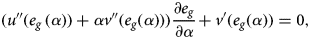 $$({u}^{\prime \prime}(e_g\,(\alpha )) + \alpha {v}^{\prime \prime}(e_g(\alpha )))\displaystyle{{\partial e_g} \over {\partial \alpha}} + {v}^{\prime}(e_g(\alpha )) = 0,$$
 $$\displaystyle{{\partial e_g(\alpha )} \over {\partial \alpha}} = -\displaystyle{{{v}^{\prime}(e_g(\alpha ))} \over {{u}^{\prime \prime}(e_g) + \alpha {v}^{\prime \prime}(e_g(\alpha ))}} \gt 0.$$
Thus the e g(α 1) > e g(α 0). Note that the household's decision on whether to have a child or not depends on the sign of
0.5(u(e b) + v(e b)) + 0.5(u(e g(α 1)) + α 1v(e g(α 1))) − u(y m + y f) − v(ξ) and if u(e g(α 1)) + α 1v(e g(α 1)) is bigger than u(e g(α 0)) + α 0v(e g(α 0)) the MU (A.1) will be positive and the household will have its first child.
Note that u(e g(α 1)) + α 1v(e g(α 1)) >u(e g(α 0)) + α 1v(e g(α 0))as e g(α 1) is optimal (utility maximizing) at α 1.
Note that u(e g(α 0)) + α 1v(e g(α 0)) >u(e g(α 0)) + α 0v (e g(α 0)).
So u(e g(α 1)) + α 1v(e g(α 1)) >u(e g(α 0)) + α 0v(e g(α 0)).
A-2. Proposition 2
Assume a household with arbitrary number of boys and girls (b, g).
Substituting
 $$c = y_m-(b + g)\,p-be_b-ge_g-y\,(1-z(b + g))$$
FOC for education are
 $$e_g{\kern 1pt} :\,\,u_{e_g}(e_b,e_g,b,g) + E\lsqb {v_{e_g}(e_b,e_g,b,g)} \rsqb = 0$$
 $$e_b{\kern 1pt} :\,\,u_{e_b}(e_b,e_g,b,g) + E\lsqb {v_{e_b}(e_b,e_g,b,g)} \rsqb = 0.$$
To know how the investment in children's human capital changes when FLFPR changes I take the full derivative of (A.3) and (A.4) with respect to α and obtain
 $$\left( {\matrix{ A & B \cr C & D \cr}} \right)\left( {\matrix{ {\displaystyle{{\partial e_g} \over {\partial \alpha}}} \cr {\displaystyle{{\partial e_b} \over {\partial \alpha}}} \cr}} \right) = \left( {\matrix{ {-a} \cr {-b} \cr}} \right),$$
where given the logarithmic assumption for u (.) and v (.) functions:
 $$A = u_{e_ge_g}(e_b,e_g,b,g) + E\lsqb {v_{e_ge_g}(e_b,e_g,b,g)} \rsqb \lt 0$$
 $$B = u_{e_ge_b}(e_b,e_g,b,g) + E\lsqb {v_{e_ge_b}(e_b,e_g,b,g)} \rsqb \lt 0$$
 $$C = u_{e_be_g}(e_b,e_g,b,g) + E\lsqb {v_{e_be_g}(e_b,e_g,b,g)} \rsqb \lt 0$$
 $$D = u_{e_be_b}(e_b,e_g,b,g) + E\lsqb {v_{e_be_b}(e_b,e_g,b,g)} \rsqb \lt 0$$
 $$a = u_{e_g\alpha} (e_b,e_g,b,g) + E\lsqb {v_{e_g\alpha} (e_b,e_g,b,g)} \rsqb $$
 $$b = u_{e_b\alpha} (e_b,e_g,b,g) + E\lsqb {v_{e_b\alpha} (e_b,e_g,b,g)} \rsqb .$$
Utility from consumption is not affected by the changes in FLFPR thus
 $$u_{e_g\alpha} (e_b,e_g,b,g) = 0$$
 $$u_{e_b\alpha} (e_b,e_g,b,g) = 0.$$
Utilizing expressions (4) and (7) from Sah (Reference Sah1991)
 $$b = E\lsqb {v_{e_b\alpha} \lpar {e_b,e_g,b,g} \rpar } \rsqb = g\sum\limits_{i = 0}^{g-1} {\alpha ^i} \left( {\matrix{ {g-1} \cr i \cr}} \right)(1-\alpha )^{g-1-i}\lpar {v_{e_b}\lpar {be_b^\gamma w + \lpar {i + 1} \rpar e_g^\gamma w} \rpar -v_{e_b}\lpar {be_b^\gamma w + ie_g^\gamma w} \rpar } \rpar \lt 0$$
If utility function v (.) is restricted to a logarithmic form
 $$v_{e_b}(be_b^\gamma w + (i + 1)\,e_g^\gamma w)-v_{e_b}(be_b^\gamma w + ie_g^\gamma w) = \displaystyle{{\gamma e_b^{\gamma -1} wb} \over {be_b^\gamma w + (i + 1)e_g^\gamma w}}-\displaystyle{{b\gamma e_b^{\gamma -1} w} \over {be_b^{ma} w + ie_g^\gamma w}} \lt 0.$$
Also,
 $$E\lsqb {v_{e_g\alpha} (e_b,e_g,b,g)} \rsqb = g\mathop \sum \limits_{i = 0}^{g-1} \alpha ^i(1-\alpha )^{g-1-i}\left( {\matrix{ {g-1} \cr i \cr}} \right)\,(v_{e_g}(be_b^\gamma w + (i + 1)e_g^\gamma w)-v_{e_g}(be_b^\gamma w + ie_g^\gamma w)).$$
If utility function v (.) is restricted to a logarithmic form
 $$v_{e_g}(be_b^\gamma w + (i + 1)e_g^\gamma w)-v_{e_g}(be_b^\gamma w + ie_g^\gamma w) = \displaystyle{{\gamma e_g^{\gamma -1} be_b^\gamma} \over {(be_b^\gamma + (i + 1)e_g^\gamma )\,(be_b^\gamma + ie_g^\gamma )}}$$
which is positive for any value of i. Thus a > 0.
If  $\left( {\matrix{ A & B \cr C & D \cr}} \right)$ is a negative definite matrix then its determinant is positive and in this case
  $\displaystyle{{\partial e_b} \over {\partial \alpha}} \lt 0$ and
  $\displaystyle{{\partial e_g} \over {\partial \alpha}} \gt 0$. The condition required for negative definite matrix is concavity of the objective function in both e b and e g which must be satisfied as it is also required for maximizing the utility function. So if optimal (utility maximizing) e b and e g exist, the matrix is negative definite.
A-3. Derivative of marginal utility from another child with respect to FLFPR
For the ease of exposition I denote  $e_b(b + 1,g,\alpha _0)\equiv e_b^b, \,e_g(b + 1,g,\alpha _0)\equiv e_g^b, \,e_b(b,g + 1, \alpha _0)\equiv e_b^g$,
  $e_g(b,g + 1,\alpha _0)\equiv e_g^g, \,e_b(b,g,\alpha _0)\equiv e_b,\,{\rm and}\,e_g(b,g,\alpha _0)\equiv e_g$. Using expressions (4) and (7) from Sah (Reference Sah1991) the derivative of marginal utility from having another child with respect to FLFPR is
 $$\eqalign{& g\sum\limits_{i = 0}^{g-1} {\alpha ^i\left( {\matrix{ {g-1} \cr i \cr}} \right)} \,(1-\alpha )^{g-1-i}(v\,(w\,(b + 1)\,(e_b^b )^\gamma + w\,(i + 1)\,(e_g^b )^\gamma )-v(w\,(b + 1)(e_b^b )^\gamma + wi\,(e_g^b )^\gamma )) \cr & \quad -g\sum\limits_{i = 0}^{g-1} {\alpha ^i\left( {\matrix{ {g-1} \cr i \cr}} \right)} \,(1-\alpha )^{g-1-i}(v\,(wb\,(e_b)^\gamma + w\,(i + 1)\,(e_g)^\gamma )-v(wb(e_b)^\gamma + wi\,(e_g)^\gamma )) \cr & \quad + (g + 1)\sum\limits_{i = 0}^g {\alpha ^i\left( {\matrix{ g \cr i \cr}} \right)} \,(1-\alpha )^{g-i}(v\,(wb(e_b^g )^\gamma ) + w\,(i + 1)\,(e_g^g )^\gamma -v\,(wb(e_b^g )^\gamma + wi\,(e_g^g )) \cr & \quad -g\sum\limits_{i = 0}^{g-1} {\alpha ^i\left( {\matrix{ {g-1} \cr i \cr}} \right)} \,(1-\alpha )^{g-1-i}(v\,(wb\,(e_b)^\gamma + w\,(i + 1)\,(e_g)^\gamma )-v(wb(e_b)^\gamma + wi\,(e_g)^\gamma )).} $$
A-4. Derivative of marginal utility from another child with respect to FLFPR (exogenous human capital of children)
Household with b boys and g girls consider having a child. Each child irrespective of gender is endowed with 1 unit of human capital. The wage per unit of human capital is assumed to be 1. Parents make decision on having another child after observing the gender outcome of the previous birth. The expected utility function (2) and budget constraint (3) simplify to
 $$U(c,b,g) = u(c) + \psi E\lsqb {v\,(b,g)} \rsqb $$
and
 $$c = y_m-(b + g)p-y\,(1-z\,(b + g)).$$
In details the expected utility function is
 $$U(c,b,g) = u\,(c) + \psi \mathop \sum \limits_{i = 0}^g \alpha ^i\left( {\matrix{ g \cr i \cr}} \right)\,(1-\alpha )^{g-i}v(b + i).$$
The decision of parents to have another child is positive if the marginal benefit from another child is positive
 $$0.5V(b + 1,g) + 0.5V(b,g + 1)-V(b,g) \gt 0.$$
To know how decision of parents changes when FLFPR increases I need to calculate the derivative of the marginal utility (A.8) with respect to α.
 $$\eqalign{&0.5\left( {\displaystyle{{\partial V(b + 1,g)} \over {\partial \alpha}} + \displaystyle{{\partial V(b,g + 1)} \over {\partial \alpha}}} \right)-\displaystyle{{\partial V(b,g)} \over {\partial \alpha}} \cr &\quad = 0.5\left( {\displaystyle{{\partial E\lsqb {v(b + 1,g)} \rsqb } \over {\partial \alpha}} -\displaystyle{{\partial E\lsqb {v(b,g)} \rsqb } \over {\partial \alpha}}} \right) + 0.5\left( {\displaystyle{{\partial E\lsqb {v\lpar {b,g + 1} \rpar } \rsqb } \over {\partial \alpha}} -\displaystyle{{\partial E\lsqb {v\lpar {b,g)} \rsqb } } \over {\partial \alpha}}} \right).} $$
Using derivations (4) and (7) from Sah (Reference Sah1991) the first part of (A.9) is
 $$\eqalign{& 0.5\left( {g\mathop \sum \limits_{i = 0}^{g-1} \alpha^i\left( {\matrix{ {g-1} \cr i \cr}} \right)\,{(1-a)}^{g-1-i}(v((b + 1) + (i + 1))-v((b + 1) + i))} \right) \cr & \quad -0.5\left( {g\mathop \sum \limits_{i = 0}^{g-1} \alpha^i\left( {\matrix{ {g-1} \cr i \cr}} \right){(1-\alpha )}^{g-1-i}(v(b + (i + 1))-v(b + i))} \right) \lt 0,} $$
as v(.) is a concave function. The second part is (A.11) and it sign is hard to identify.
 $$\eqalign{& 0.5\left( {(g + 1)\mathop \sum \limits_{i = 0}^g \alpha^i\left( {\matrix{ g \cr i \cr}} \right)\,{(1-a)}^{g-i}(v((b + 1) + (i + 1))-v((b + 1) + i))} \right) \cr & \quad -0.5\left( {g\mathop \sum \limits_{i = 0}^{g-1} \alpha^i\left( {\matrix{ {g-1} \cr i \cr}} \right)\,{(1-\alpha )}^{g-1-i}(v(b + (i + 1))-v(b + i))} \right) \lessgtr 0.} $$
A-5. Intermediate result 1
The extreme case of a household which has b boys and considers having another child. It is known that the next child will be a girl. The household will decide to have an additional child if marginal utility (A.12) is positive.
 $$MU = u\,(e_{b1},e_{g1},b,1) + \alpha v\,(e_{b1},e_{g1},b,1) + (1-\alpha )v\,(e_{b1},0,b,1)-u(e_{b0},0,b,0)-v(e_{b0},0,b,0),$$
where e b1 and e g1 are investment in education of boys and a girl if household decides to have a girl, e b0 is the investment in education of boys if the household abstains from having that girl and v (e b1, 0, b, 1) means a household has b boys and a girl, the boys work, so the household derives utility from their e b1 while a girl does not work, hence instead of e g1 we have 0.
The full derivative of the MU (A.12) with respect to α is expression (A.13) (note that utility with b boys does not depend on α so its derivative with respect to α is zero)
 $$\eqalign{MU_\alpha &= (u_{e_b}(e_{b1},\,e_{g1},\,b,\,1) + \alpha v_{e_b}(e_{b1},\,e_{g1},\,b,\,1) + (1-\alpha )\,v_{e_b}\,(e_{b1},0,b,1))\displaystyle{{\partial e_b} \over {\partial \alpha}} \cr &\quad + (u_{e_g}(e_{b1},\,e_{g1},\,b,\,1) + \alpha v_{e_g}(e_{b1},\,e_{g1},\,b,\,1) + (1-\alpha )\,v_{e_g}\,(e_{b1},0,\,b,\,1))\displaystyle{{\partial e_g} \over {\partial \alpha}} \cr & \quad + (u_\alpha (e_{b1},\,e_{g1},\,b,\,1) + v\,(e_{b1},\,e_{g1},\,b,\,1)-v\,(e_{b1},\,0,\,b,\,1)).} $$
Note that first two lines of derivative of marginal utility with respect to α (A.13) are FOC for the optimal education choice in case of b boys and 1 girl which is a result from the Envelope Theorem stating that the first two lines of (A.13) are zero and only direct effect of α matters. The u α(e b1, e g1, b, 1) is zero too as consumption part of the utility function does not directly depend on α. Thus the full derivative of the marginal utility with respect to α (A.14) is positive.
 $$v\,(e_{b1},e_{g1},b,1)-v\,(e_{b1},0,b,1).$$
When the next child is known to be a boy the utility does not depend on α, so marginal utility from having another child is not affected by FLFPR.
A-6. Exogenous human capital case all-boy households
In the all-boy household decides to have a child and the child gender is stochastic, the marginal utility from having another child is
 $$\eqalign{& \alpha \,(u\,(y_m-(b + 1)\,p + LF\cdot y_f\,(1-z\,(b + 1))) + v\,(b + 1) \cr & \quad\quad\qquad + (1-\alpha )\,(u\,(y_m-(b + 1)\,p + LF\cdot y_f\,(1-z\,(b + 1))) + v\,(b))) \cr & \quad\quad\qquad -u\,(y_m-bp-LF\cdot y_f\,(1-zb))-v\,(b) \cr & \quad\quad\qquad = u\,(y_m-(b + 1)p + LF\cdot y_f\,(1-z(b + 1))) \cr & \quad\quad\qquad -u\,(y_m-bp-LF\cdot y_f\,(1-zb)) + \alpha \,(v\,(b + 1)-v\,(b)).} $$
When α increases, it is obvious that marginal benefit (third term of expression (A.15) after the equation sign) will increase while marginal cost (first two terms of the expression) will not change.
A-7. Intermediate result 2
The extreme case of household which has g girls and considers to have another child who is known to be a boy. The household will decide to have that child if marginal utility from having that child is positive.
The marginal utility is
 $$MU = u(c_1) + E\lsqb {v\,(e_{b1},\,e_{g1},\,1,\,b)} \rsqb -u\,(c_0)-E\lsqb {v\,(0,e_{g0},0,g)} \rsqb .$$
where e b1, e g1, and c 1 are investment in human capital of a boy and girls and household consumption if the household decides to have another child while e g0 and c 0 are the investment in human capital of girls and household consumption if the household abstains from having another child.
The full derivative of the MU (A.16) with respect to α is
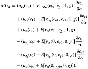 $$\eqalign{MU_\alpha &= (u_{e_b}(c_1) + E[v_{e_{b1}}(e_{b1},e_{g1},1,g)]\displaystyle{{\partial e_{b1}} \over {\partial \alpha}} \cr &\quad + (u_{e_g}(c_1) + E[v_{e_{g1}}(e_{b1},e_{g1},1,g)]\displaystyle{{\partial e_{g1}} \over {\partial \alpha}} \cr &\quad + (u_\alpha (c_1) + E[v_\alpha (e_{b1},e_{g1},1,g)] \cr &\quad-(u_{e_{_b}} (c_0) + E[v_{e_b}(0,e_{g0},0,g)]\displaystyle{{\partial e_b} \over {\partial \alpha}} \cr &\quad-(u_{e_g}(c_0) + E[v_{e_{g0}}(0,e_{g0},0,g)]\displaystyle{{\partial e_{g0}} \over {\partial \alpha}} \cr &\quad -(u_\alpha (c_0) + E[v_\alpha (0,e_{g0},0,g)]).} $$
The first, second, fourth, and the fifth lines of derivative (A.17) are zero as they are FOCs for the optimal choice of education and consistent with the Envelope Theorem stating that we must consider only direct effect of α . Thus,
 $$MU_\alpha = u_\alpha \,(c_1) + E\lsqb {v_\alpha \,(e_{b1},e_{g1},1,g)} \rsqb -u_\alpha (c_0)-E\lsqb {v_\alpha \,(0,e_{g0},0,g)} \rsqb .$$
Using expressions (4) and (7) from Sah (Reference Sah1991) and the fact that u(.) does not depend on α, the expressions (A.18) is
 $$\eqalign{MU_\alpha &= g\sum\limits_{i = 0}^{g-1} {\alpha ^i} \lpar {1-\alpha} \rpar ^{g-1-i}\left( {\matrix{ {g-1} \cr i \cr}} \right)\lpar {v\lpar {e_{b1}^\gamma w + \lpar {i + 1} \rpar e_{g1}^\gamma w} \rpar -v\lpar {e_{b1}^\gamma w + ie_{g1}^\gamma w} \rpar } \rpar \cr & \quad -g\sum\limits_{i = 0}^{g-1} {\alpha ^i} \lpar {1-\alpha} \rpar ^{g-1-i}\left( {\matrix{ {g-1} \cr i \cr}} \right)\lpar {v\lpar {\lpar {i + 1} \rpar e_{g0}^\gamma w} \rpar -v\lpar {ie_{g0}^\gamma w} \rpar } \rpar .} $$
If the utility function v(.) is restricted to be logarithmic then
 $$MU_\alpha = g\sum\limits_{i = 0}^{g-1} {\left( {\matrix{ {g-1} \cr i \cr}} \right)} {\rm ln}\left( {\displaystyle{{e_{b1}^\gamma ie_{g0}^\gamma + i^2e_{g1}^\gamma e_{g0}^\gamma + e_{g1}^\gamma ie_{g0}^\gamma} \over {e_{b1}^\gamma ie_{g0}^\gamma + e_{b1}^\gamma e_{g0}^\gamma + i^2e_{g1}^\gamma e_{g0}^\gamma + e_{g1}^\gamma ie_{g0}^\gamma}}} \right),$$
the argument in the logarithm in the marginal utility (A.19) less than 1 for any i > 0 which means that derivative of marginal utility with respect to α (A.18) is negative.
A-8. Intermediate result 3
The extreme case is when a household with g girls consider having another child, when that child is known to be a girl. This is a bit complicated as both the “flow” and the “stock” effects are operational in this case. To simplify derivations and see how marginal utility changes imagine parents must make a one-time decision on number of children (all of whom are girls) they want to have and amount investment in their human capital formation. When we have all-girl household who will have a girl one time decision making on number of children who are all girls is an accurate depiction of reality. This is true as one may imagine that before making final one-time decision, a household, as standard utility maximizer, weights the costs and the benefits of an additional child, so in its calculations, one-time decision making household follows a sequential decision making. The u(.) and v(.) functions are logarithmic. The FLFPR they observe is α. So the household problem is
 $${\rm ma}{\rm x}_{g,e}\mathop \sum \limits_{i = 0}^g \left( {\matrix{ g \cr 0 \cr}} \right)\alpha ^i(1-\alpha )^{g-i}({\rm ln}(y_m-(\,p + e)g + y_f\,(1-zg)) + {\rm ln}(iwe^\gamma )).$$
Following Kalemli-Ozcan (Reference Kalemli-Ozcan2003) the utility can be approximated around expected number of surviving children using Delta method:
 $${\rm ma}{\rm x}_{g,e}{\rm ln}(y_m-(\,p + e)g + y_f\,(1-zg)) + {\rm ln}(g\alpha we^\gamma )-\displaystyle{{(1-\alpha )} \over {2g\alpha}} $$
Kalemli-Ozcan (Reference Kalemli-Ozcan2003) has shown that fertility is decreasing in child survival rate, which is equivalent to fertility decreasing in FLFPR, however I provide an alternative way to see this. For simplicity I will denote the total utility as one part coming from consumption and another part coming from children
 $${\rm ma}{\rm x}_{g,e}\lcub {u + v} \rcub .$$
The FOC are:
 $$e:\,u_e + v_e = 0 \;{\rm and}\; g:\,\,u_g + v_g = 0$$
If I totally differentiate the FOC with respect to FLFPR (α) I will have
 $$\left( {\matrix{ A & B \cr C & D \cr}} \right)\left( {\matrix{ {\displaystyle{{\partial e} \over {\partial \alpha}}} \cr {\displaystyle{{\partial g} \over {\partial \alpha}}} \cr}} \right) = \left( {\matrix{ {-a} \cr {-b} \cr}} \right),$$
where A = u ee + v ee, B = u eg + v eg, C = u ge + v ge, D = u gg + v gg, a = u eα + v eα, b = u gα + v gα.
Note that a = 0 as e eα = 0 and v eα = 0, as well as u gα = 0, v eg = 0, u eg <0, u ee <0, v ee <0,
and
 $$v_{g\alpha} = -\displaystyle{1 \over 2}\displaystyle{{(1-\gamma )} \over {g^2\alpha}} -\displaystyle{1 \over 2}\displaystyle{{(1-\gamma )(1-\alpha )} \over {g^2\alpha ^2}} \lt 0.$$
Keeping in mind that in order to have a local maximum the Hessian should be negative definite, for 2 × 2 case the determinant of Hessian should be positive. Thus
 $$\displaystyle{{\partial g} \over {\partial \alpha}} \lt 0$$
 $$\displaystyle{{\partial e} \over {\partial \alpha}} \gt 0.$$
Thus, the marginal utility from an additional child decreases in FLFPR (A.22).
A-9. Exogenous human capital case
I assume for simplicity that human capital and wage per unit of human capital are equal to 1. Imagine a household with g girls which is considering having another child, who is known to be a boy. Note that in this setup, changes in FLFPR does not affect return from the additional child, it affects only already existing girls. The marginal utility from having another child is
 $$(u\,(y_m-(g + 1)p + y_f\,(1-zg)) + v\,(g + 1))-(u\,(y_m-gp + (1-zg))-v\,(g)).$$
The derivative of expression (A.24) with respect to FLFPR is expression (A.10) if b = 1. So independent on number of girls, at any level of FLFPR the derivative is negative.
In the case when the next child is known to be a girl the cross derivative of the utility function (approximated by Delta method as in Appendix A-8) with respect to g and α is:
in case of logarithmic utility
 $$\displaystyle{{\partial ^2U} \over {\partial g\partial \alpha}} = -\displaystyle{1 \over {2g^2}}\,(\alpha ^{-1} + \alpha ^{-2}(1-\alpha )) \lt 0,$$
in case of CRRA function
 $$\displaystyle{{\partial ^2U} \over {\partial g\partial \alpha}} = \left( {(1-\beta )\,{(g\alpha )}^{-\beta} -\displaystyle{{\beta^2} \over {2g^{\beta + 1}}}\,(\alpha^{-\beta} + \beta \alpha^{-\beta -1}\,(1-\alpha ))} \right).$$
Here as well as in Kalemli-Ozcan (Reference Kalemli-Ozcan2003) logarithmic function (A.25) is such that substitution and income effects coming from increase in expected return are canceling each other leaving only the variance effect (precautionary saving reduction). For other utility functions (for example CRRA function with coefficient of relative risk aversion β) the income and substitution effects may not cancel and actually fertility may increase like if β < 1 while at β > 1 (A.26) this derivative is always negative.
Given the results for  $\displaystyle{{\partial ^2U} \over {\partial g\partial \alpha}} $ it is clear that in logarithmic case the change in marginal benefit is negative (in case of CRRA utility function when β < 1 it can be positive as mean effect can outweigh the variance effect). Thus, for fairly concave utility function, marginal benefit from having additional child decreases while marginal cost associated with that child does not change. This means that household who at lower FLFPR found it optimal to have another child, at higher FLFPR may find it non-optimal.
A-10. General utility functions
As stated above, in the settings where some of the children have a chance of not working, and thus deriving no utility from them, the model resembled models which study the effect of child survivability. The analogy (which is obviously very crude) worked well in utilizing the results established in that literature. In fact, in the initial version of this study, which is purely a numerical exercise, each child (daughter) who ended up not in the labor force was delivering to the parental utility some constant χ and it looked like 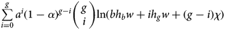 $\mathop \sum \limits_{i = 0}^g a^i(1-\alpha )^{g-i}\left( {\matrix{ g \cr i \cr}} \right){\rm ln}(bh_bw + ih_gw + (g-i)\chi )$. This was done not only to be more realistic (so parents value children no matter their future labor status), but also to avoid complications in numerical solutions with logarithmic functions, because if none of the g daughters earned income, this would mean (1 − α)gln(0), which obviously was not helping the solution. As I moved to theoretical derivations and switched to using the CRRA function (so I can play with its curvature parameter), (1 − α)g((0)1−σ/(1 − σ)) was no longer a computational problem, and I stopped adding that constant to make analytical derivations easier. I tried to choose the simplest possible approach to illustrate the “hoarding” of children due to the SP-DSB and the interaction of “stock” and “flow” effects when the FLFPR changes.
To add more context for my choice of utility function, please note that parents do not derive utility from the discounted lifetime stream of income, but rather from the earning per unit of time  $(e_i^\gamma w)$, which is a way to quantify the “earning potential” of each child. This “earning potential” stays as a sign of indirect utility, an indication of the tightness of the budget constraint that children will be facing. In this setting, obviously, the valuation of the investment in children and its quantity depend whether children are expected (likelihood) to realize those investments into earning (be in the labor market).
In general, we can assume that children contribute to their parents utility in two ways: as children-delivering “pure joy” to altruistic parents (possible dependent on the total human capital, indicating a certain combination of child quality and quantity), and as children earning income (being in the labor market), which can be thought of as the indirect utility discussed above. I have already stated that one may normalize the generic components of having children to 0, assuming that the intrinsic valuation of children is not different between genders. However, to stay in a more general setup, and to show that the main results are not just due to the particular form of utility function choice, I will present the results for three alternative (general) utility functions. They are more general in the sense that parents derive utility from children independent of their future labor force status, e.g., something we can refer to as “pure joy,” pleasure of having children. For all three specifications, I tried to stay close to the original calibration parameters, and for the newly introduced parameters, I could easily find parameters, which would generate similar stopping rules observed in the baseline version of the model.
Specification 1.
 $$U_j(c,e_b,e_g,b,g) = u\,(c) + z\,(b + g) + \psi \mathop \sum \limits_{i = 0}^g a^i(1-\alpha )^{g-i}\left( {\matrix{ g \cr i \cr}} \right)v\,(be_b^\gamma w_m + ie_g^\gamma w_f).$$
Before going to the numerical results, let me note that this specification does not affect the interaction of the “flow” and “stock” effects due to the fact that z (b + g) does not depend on the FLFPR. Thus, in the calculation of the effect of the FLFPR on the marginal utility from the additional child (derivative of the marginal utility), z (b + g)Footnote 20 will be zero.
The parameters used in the exercise are: ψ = 0.19, φ = 0.02Footnote 21. Note that I had to introduce a parameter φ in front of z (b + g), otherwise the mean number of children was beyond any reasonable number. This specification introduces sluggishness in the results (which increases in φ), the variation of the stopping rule is less elastic to changes in the FLFPR, but the changes themselves are consistent with the “flow” and “stock” effects. So, it is still possible to obtain more or less similar stopping rules as in the baseline model, with extreme case of son-preference at low levels of FLFPR and the “flow” and “stock” effects becoming apparent as the FLFPR increases (Table A.1).
Specification 2.
 $$U_j(c,e_b,e_g,b,g) = u\,(c) + \psi \mathop \sum \limits_{i = 0}^g a^i(1-\alpha )^{g-i}\left( {\matrix{ g \cr i \cr}} \right)v\,(\kappa \lsqb {I(b + g)} \rsqb + (1-\kappa )\lsqb {be_b^\gamma w_m + ie_g^\gamma w_f} \rsqb ).$$
 Recall that in my description I speak about the “pure joy” of having children component in the utility function (let us denote it by I) from children being normalized to 0. However, to maintain this generic form, I can assume I = 1. Note that when the weight on the “pure joy” from children is weighted by κ = 0 we are back to the original utility I used before. As stated, I suggest to have a more generalized way of assuming that the return of a girl consists of two components, the generic one, where parents simply enjoy the daughter, and the component that is related to her income, “earning potential.” In this specification, the analog z (b + g) in Specification 1, is inserted into the 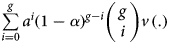 $\mathop \sum \limits_{i = 0}^g a^i(1-\alpha )^{g-i}\left( {\matrix{ g \cr i \cr}} \right)v\,(.)$ function. This makes the effect of the FLFPR on marginal utility depend on the “pure” joy of having children. So I can assume that parents derive utility from a linear combination of “pure” joy from total number of children and their total income;
  $\kappa \lsqb {I(b + g)} \rsqb + (1-\kappa )\lsqb {be_b^\gamma w_m + ie_g^\gamma w_f} \rsqb $.
The results of this numerical estimation are in Table A.2. The parameters used in the exercise are: ψ = 0.25, κ = 0.2, I = 0.05, y f = 0. Even in the case when the “pure joy” of having children is in the utility function v (.), at parameters values so that we have a reasonable TFR, we observe extreme “son-preference” at low levels of FLFPR and the effects of the “flow” and “stock” effects when the FLFPR is higher.
Specification 3.
To simplify notation, I can propose a more compact, but very similar way of modeling preference for children
 $$U_j(c,e_b,e_g,b,g) = u\,(c) + \psi \mathop \sum \limits_{i = 0}^g a^i\,(1-\alpha )^{g-i}\left( {\matrix{ g \cr i \cr}} \right)v\,(be_b^\gamma w_m + e_g^\gamma (\kappa \cdot i + (1-\kappa )g)w_f),$$
where utility from children comes from a linear combination of their human capital (scaled by wage) as an indicative of higher culture, reading, enjoying intellectual life, being a more educated mother or father (“pure joy”), and the components coming from being in the labor market. Because I assume for boys, labor force participation is sure, we have just  $be_b^\gamma w_m$ for boys. For girls, however, as g and i are not necessary the same, we have
 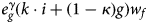 $e_g^\gamma (k\cdot i + (1-\kappa )g)w_f$.
The results of this numerical estimation are in Table A.3. The parameters used in the exercise are: ψ = 0.24, κ = 0.7, y f = 0. As expected, the stopping rules resulting from this modeling specifications are closest to the baseline results due to the similarity of the specifications. As in the two previous experimental cases, at a low FLFPR we observe the extreme case of “son-preference,” which is weakened at a higher FLFPR when we start to observe the “flow” effect. The extremely large family size also decreases at a higher FLFPR due to the “stock” effect.
This section shows that in the numerical exercise, although the relative strength of the interaction between “flow” and “stock” effects change for different utility specifications, calibrations yielding fertility stopping rules similar to the baseline version are easy to find.
A-11. Fertility stopping rules of type II households with general utility functions
Table A.1. Fertility stopping rules of type-II households; general utility function, specification 1

Table A.2. Fertility stopping rules of type-II households; general utility function, specification 2

Table A.3. Fertility stopping rules of type-II households; general utility function, specification 3