


1. INTRODUCTION
The difference between the EU15 and US unemployment rates in recent decades is well known. European unemployment was low during the 1960s but started to increase in the 1970s, and rose above the US rate in the early 1980s, where it has remained ever since. This phenomenon is often referred to as the EU–US unemployment puzzle. The earlier literature, starting with Nickell (Reference Nickell1997), often emphasized the role of changes in labor-market institutions (LMIs) to explain this gap. In particular, this literature showed that greater institutional rigidities are a central cause of Europe’s bleak unemployment performance. Aging may also affect unemployment. In the overlapping-generations (OLG) approach, life expectancy typically stimulates savings [e.g., Attanasio et al. (Reference Attanasio, Kitao and Violante2007)]. In closed economies, higher savings automatically generate investment, which reduces unemployment. This is the main finding of de la Croix et al. (Reference de la Croix, Pierrard and Sneessens2013). As a result, a fast-aging area such as Europe should experience a low unemployment rate, all else equal, a finding at odds with the puzzle mentioned above. However, in an open-economy framework, capital mobility may blur this savings-investment link [see for instance, Flodén (Reference Flodén2003), Domeij and Flodén (Reference Domeij and Flodén2006), and Börsch-Supan et al. (Reference Börsch-Supan, Ludwig and Winter2006)] and, hence, that between aging and unemployment when countries are characterized by differential aging. In this paper, we investigate how each of LMIs, aging, and capital flows contribute to the EU–US unemployment gap.
We first construct a two-period two-region general-equilibrium model with OLG dynamics. To generate unemployment, we follow the search and matching literature [Pissarides (Reference Pissarides2000)] and allow capital to move – or not – between regions. We use this model to demonstrate analytically the implications of LMIs (here unemployment- and pension-replacement rates), fertility and aging on savings, (un)employment and capital flows. We then set up a quantitative model with a larger number of generations and endogenous labor supply. We calibrate this model using EU15 and US data and also feed in the historical and projected changes in (i) LMIs and (ii) demography. We quantitatively assess its ability to explain the observed changes in the individual (EU15 vs. US) unemployment rates between 1960 and 2010, as well as the unemployment-rate gap.Footnote 1
Our main findings can be summarized as follows. First, institutional features alone, i.e., the asymmetric strengthening of LMIs with an EU15 bias, reproduces changes in the individual unemployment rates between 1960 and 2010, and that in the gap, reasonably well. The average error (between the observed and simulated data) for the individual unemployment rates is 0.9 percentage points (pp) and that for the gap is 1.1 pp. Adding demographic changes in closed economies, i.e., asymmetric aging with a EU15 bias, worsens the fit: the relatively higher savings in the EU reduce the real interest rate, which stimulates job creation and lowers unemployment. However, introducing open economies allows capital to flow from Europe to the US and this lowers EU unemployment that is, in some sense, exported. This final model (with institutions, demography, and capital flows) performs the best, with the average error for the individual unemployment rates becoming 0.8 pp and that for the gap 0.9 pp Second, although the model performs well in terms of unemployment, it does exaggerate the extent of capital flows. We therefore introduce restrictions on capital mobility to exactly match the historical change in EU–US net foreign assets (NFAs). The unemployment fit remains almost as good as in the frictionless model. We also discuss extensions with possible implications for savings and capital flows, such as capital taxes, an imperfect annuity market, and the introduction of a third region. Third, we extend the horizon to understand the effects of major institutional and demographic changes between 2010 and 2050: the stabilization of the size of LMIs in the two regions and the substantial start of the aging process in the US.
This paper relates to the debate over the role of institutions in the historical rise in the EU15–US unemployment gap. There is much empirical controversy regarding this question. On the one hand, Nickell et al. (Reference Nickell, Nunziata and Ochel2005) emphasize the role of changes in LMIs to explain this gap, and also show that interactions between the average values of institutions and shocks do not improve our understanding of this gap. On the other hand, Blanchard and Wolfers (Reference Blanchard and Wolfers2000) argue that institutional changes are not central for the explanation of the stylized facts (European countries already enjoyed well-developed welfare systems before the rise in the gap), but it is rather the interaction between common shocks and different institutional levels. We contribute to this discussion. We first show that asymmetric LMI changes only, that is without aging and capital mobility, can reproduce a large part of the historical rise in the EU15–US unemployment gap. This is in line with Nickell et al. (Reference Nickell, Nunziata and Ochel2005). Second, we show that this result no longer holds when we add asymmetric aging to asymmetric institutional changes (keeping capital mobility unchanged). Third, we are able to restore and even improve upon the initial result when we allow for international capital mobility. This paper also relates to work that considers the general-equilibrium OLG approach to be the appropriate way of quantifying the international implications of demographic changes and, in particular, differential aging [for example, Fehr et al. (Reference Fehr, Jokisch and Kotlikoff2003), Börsch-Supan et al. (Reference Börsch-Supan, Ludwig and Winter2006), Attanasio et al. (Reference Attanasio, Kitao and Violante2007), and Krueger and Ludwig (Reference Krueger and Ludwig2007)]. One of the main findings in this literature is that capital mobility (largely induced by demographic differences) affects factor prices, macroeconomic variables, and the distribution of wealth. In the receiving country, capital inflows boost labor income (which enhances the welfare of young workers) and reduce capital returns (which harms the elderly). Labor markets are, however, assumed to be competitive, so that there is no effect on unemployment. To our knowledge, there are only two papers using general equilibrium models with OLG dynamics and labor-market frictions to consider demographic changes. Jaag et al. (Reference Jaag, Keuschnigg and Keuschnigg2010) analyze the effects of a pension reform in Austria and de la Croix et al. (Reference de la Croix, Pierrard and Sneessens2013) look at the effects of aging on unemployment. However, both use closed-economy models. This paper is closely related to de la Croix et al. (Reference de la Croix, Pierrard and Sneessens2013). The main difference is that we have two open economies with international capital mobility instead of one closed economy. This has important consequences. In de la Croix et al. (Reference de la Croix, Pierrard and Sneessens2013), aging stimulates savings and therefore capital accumulation. Real interest rates fall, which encourages job creation and reduces unemployment. In our work, the link between savings and capital accumulation is broken, and therefore so is that between aging and unemployment.
The remainder of this paper is organized as follows. Section 2 presents empirical evidence on asymmetric institutions and aging between the EU15 and the US, bilateral capital flows and the gap in the unemployment rate. In Section 3, we develop a simple, analytically tractable multi-country OLG model to highlight the qualitative effects of LMIs and demographic differences on capital flows and unemployment. We use these analytical results in the subsequent analysis to better understand the quantitative results. Section 4 describes the quantitative model and Section 5 sets out the calibration. In Section 6, we present the key simulation results, underlining the roles of institutions, demography, and capital flows in explaining the EU and US unemployment rates. Section 7 extends the horizon beyond 2010 and Section 8 concludes.
2. FACTS
The difference in EU15 and US unemployment performance over recent decades is well known. European unemployment was low during the 1960s but started to increase in the 1970s. It rose above the US level in the early 1980s and has remained higher ever since (see panel a in Figure 1).Footnote 2 The EU15–US unemployment gap mostly widened from 1960 onwards, rising from around −4% in 1960 to almost 5% in 1995 (panel b), but then declining to 1% in 2010.

Figure 1. EU15–US labor markets, demography, and net foreign asset position. Panel a, “Unemployment rate”: Unemployment rate of 25–54 year olds. 5-year smoothed average (e.g., 2005 = the 2003 to 2007 average). The data are from the OECD. Panel b, “UR gap”: Unemployment-rate gap. Calculated as the difference between the EU15 and US unemployment rates. A negative (resp. positive) number means that the EU15 unemployment rate is lower (higher) than that in the US. “NFA gap”: Net Foreign Assets gap. Calculated as the difference between US-owned assets (excluding financial derivatives) in the EU15 and EU15-owned assets (excluding financial derivatives) in the US, divided by US GDP. A positive sign (resp. negative) means that the US is a net creditor (debtor). The data are from the Bureau of Economic Activity. The figures are normalized to zero in 1960. No data are available before 1960. Panel c: Relative retirement- and unemployment-replacement rates. Calculated as the difference between EU15 and US replacement rates. A positive number indicates that EU institutions are more generous than their US counterparts. Panel d: The dependency ratio is the percentage of people aged 65+ years over people aged 25–64 years. The working-age population ratio is the percentage of people aged 25–64 years over people aged 25+ years. The data are from the United Nations.
A number of other aspects of the economy have also evolved in an asymmetric fashion in recent decades. First, LMIs, depicted in panel c of Figure 1 and measured by unemployment and retirement replacement rates, have always been stronger in the EU15 than in the US. Moreover, this gap grew between 1960 and 2005. According to OECD data including recent reforms, the retirement replacement rates are currently falling. Second, while the old-age dependency ratio in the US was almost constant between 1960 and 2010, it increased from 15% to 25% in Europe, as shown in panel d of Figure 1. Similarly, the working-age ratio fell by 7 pp in the EU15 over the same period, but by only 2 pp in the US. Third, the capital flows from the EU15 to the US (panel b) from 1960 onwards reveal a deterioration in the US NFA position with Europe.
There are, therefore, some striking similarities between the movements in relative LMI and the unemployment-rate gap, with a steady rise starting in 1960 followed more recently by a small drop. At the same time, we also observe a parallel between relative aging and the direction of net capital flows. Last, the unemployment-rate gap and capital flows might themselves be related [see, for instance, Head and Smits (Reference Head and Smits2004)]. To examine all of these possible links, we first develop a simple analytically tractable OLG model. We then adopt a numerical general-equilibrium model to quantify the international implications of LMIs and demographic changes on capital flows and labor-market outcomes in both a historical and forward-looking perspective.
An alternative way of looking at the different relationships between aging, LMIs, capital flows, and unemployment over the 1960–2010 period is via econometrics. One advantage of the econometric approach is that it can statistically assess whether the storyline suggested above is valid. The difficulty here would certainly be to appropriately and convincingly identify the many different causal relationships. By way of contrast, a dynamic general-equilibrium model provides a framework in which the different interactions are generated endogenously and dynamically. Moreover, our model with search and matching frictions also has the advantage of providing a theoretical foundation for the functioning of labor markets. Last, the OLG framework calibrated on official LMIs and demographic data can incorporate various types of institutions (benefits for the unemployed, retired, and early retired) and detailed demographic information reproducing, for example, a time-varying age pyramid over a given time period.
3. A STYLIZED MODEL
Section 2 underlined that between 1960 and 2010, (i) LMIs, measured by unemployment and pension replacement rates, were more developed in the EU15 than in the US and (ii) the aging process accelerated more in the EU15 than in the US. At the same time, capital migrated from Europe to the United States, and the EU–US unemployment gap rose (at least until 1995).
This section aims to provide qualitative insights into the combined effects of these asymmetric developments in LMIs and population aging. To do so, we construct a stylized two-period, two-country OLG model that can be solved analytically. Population aging is introduced via changes in the survival probability or fertility rate, and LMIs are measured by the generosity of public unemployment and pension benefits. The setup is a search and matching model with exogenous job destruction with or without capital mobility. We first focus on a closed-economy model, i.e., no capital mobility, and then consider the consequences of perfect capital mobility in a two-country model.
3.1. Closed Economies
Demography and labor flows
Each generation lives for up to two periods. The size of the new generation increases at a rate of f; the size of the old generation is a fraction θ of that of the corresponding young generation, where 0 < θ < 1 is the survival probability. The size of the total population scaled by the size of the new generation is thus
 $$\begin{equation*}
\frac{N_t}{N^y_t} = 1+\theta \phi ,
\end{equation*}$$
$$\begin{equation*}
\frac{N_t}{N^y_t} = 1+\theta \phi ,
\end{equation*}$$
where
 $\phi \equiv \frac{1}{1+f}\le 1.$
A larger survival probability or lower fertility rate both imply a higher old-age dependency ratio. Young households supply one unit of labor and use their labor income to pay taxes, consume, and save. In period two, the surviving households retire and consume their savings and pension benefits.
$\phi \equiv \frac{1}{1+f}\le 1.$
A larger survival probability or lower fertility rate both imply a higher old-age dependency ratio. Young households supply one unit of labor and use their labor income to pay taxes, consume, and save. In period two, the surviving households retire and consume their savings and pension benefits.
Frictions on the labor market generate imperfections and unemployment. Employment is determined by a standard matching function. In this two-period setup where only the young generation participates in the labor market, employment is equal to the number of matches:
 $$\begin{equation}
n_t = \bar{m}\,v_t^\nu ,\hspace{14.22636pt}\mbox{where}\;\bar{m}> 0,\;0\le \nu \le 1.
\end{equation}$$
$$\begin{equation}
n_t = \bar{m}\,v_t^\nu ,\hspace{14.22636pt}\mbox{where}\;\bar{m}> 0,\;0\le \nu \le 1.
\end{equation}$$
Here, n
t
is the employment rate,
 $\bar{m}$
is a matching-efficiency parameter, vt
is the number of vacancies per worker at the beginning of period t, and ν is the elasticity of matches with respect to vacancies.
$\bar{m}$
is a matching-efficiency parameter, vt
is the number of vacancies per worker at the beginning of period t, and ν is the elasticity of matches with respect to vacancies.
Households
We assume the following lifetime expected-utility function:
 $$\begin{equation}
\ln c^y_t + \beta \theta \ln c^o_{t+1},\hspace{14.22636pt}\mbox{where}\;0<\beta <1.
\end{equation}$$
$$\begin{equation}
\ln c^y_t + \beta \theta \ln c^o_{t+1},\hspace{14.22636pt}\mbox{where}\;0<\beta <1.
\end{equation}$$
Here, cy t and co t + 1 stand for the consumption of the young and the old, respectively. The utility of future consumption is weighted by the subjective discount factor β.Footnote 3 The employed member of a young household earns a wage of w t , and pays taxes at the rates of τ r t to finance retirement benefits and τ u t to finance (untaxed) unemployment benefits of bu t . In the second period, all surviving households retire and receive (untaxed) pension benefits br t + 1. If we further assume that households have access to perfect annuity markets, optimal consumption results from the maximization of expected lifetime utility (2) subject to the employment constraint (1) and the following intertemporal budget constraint:
 $$\begin{equation}
c^y_t+\theta \,\frac{c^o_{t+1}}{1+r_{t+1}} = \left(1-\tau ^r_t-\tau ^u_t\right) w_t n_t+ b^u_t(1-n_t)+\theta \,\frac{b^r_{t+1}}{1+r_{t+1}},
\end{equation}$$
$$\begin{equation}
c^y_t+\theta \,\frac{c^o_{t+1}}{1+r_{t+1}} = \left(1-\tau ^r_t-\tau ^u_t\right) w_t n_t+ b^u_t(1-n_t)+\theta \,\frac{b^r_{t+1}}{1+r_{t+1}},
\end{equation}$$
where r t + 1 is the real interest rate. The first-order condition, the Euler equation, is
 $$\begin{equation}
c^o_{t+1} = \beta (1+r_{t+1})\;c^y_t.
\end{equation}$$
$$\begin{equation}
c^o_{t+1} = \beta (1+r_{t+1})\;c^y_t.
\end{equation}$$
Combining the Euler equation and the budget constraint yields the following savings equation:
 $$\begin{eqnarray}
s_t = \frac{\beta \,\theta }{1+\beta \,\theta }\left\lbrace \left(1-\tau ^r_t-\tau ^u_t\right)\,w_t\,n_t + b^u_t\,(1-n_t)-\,\frac{b^r_{t+1}}{\beta \,\left(1+r_{t+1}\right)}\right\rbrace ,
\end{eqnarray}$$
$$\begin{eqnarray}
s_t = \frac{\beta \,\theta }{1+\beta \,\theta }\left\lbrace \left(1-\tau ^r_t-\tau ^u_t\right)\,w_t\,n_t + b^u_t\,(1-n_t)-\,\frac{b^r_{t+1}}{\beta \,\left(1+r_{t+1}\right)}\right\rbrace ,
\end{eqnarray}$$
where s t stands for the savings per worker.
Government
The government balances its budget in every period and finances both the pay-as-you-go pension system and unemployment benefits via payroll taxes, which implies
 $$\begin{equation}
b^u_t\,(1-n_t) = \tau ^u_{t}\,n_{t}\;w_{t},\\
\end{equation}$$
$$\begin{equation}
b^u_t\,(1-n_t) = \tau ^u_{t}\,n_{t}\;w_{t},\\
\end{equation}$$
 $$\begin{equation}
b^r_{t+1} = \frac{\tau ^r_{t+1}}{\theta \phi }\,n_{t+1}\;w_{t+1}.
\end{equation}$$
$$\begin{equation}
b^r_{t+1} = \frac{\tau ^r_{t+1}}{\theta \phi }\,n_{t+1}\;w_{t+1}.
\end{equation}$$
We assume a constant τ r t = τ r as well as a constant net unemployment benefit rate of ρ u , i.e., bu t = ρ u (1 − τ r t − τ u t ) wt . The values of τ r and ρ u measure the generosity of public pension and unemployment benefits.
Firms
Firms have a Cobb–Douglas production technology with 0 < α < 1. They rent capital k
t
and labor n
t
from the households and face a cost for each posted vacancy. In line with the existing literature, we assume that the cost per vacancy is proportional to total factor productivity [see for instance, Pissarides (Reference Pissarides2000), Chap. 3]. As our focus is on demographics rather than technological progress, we will assume that total factor productivity is constant. The cost per vacancy is thus constant too and will be denoted by
 $\mathsf{a} >0$
.
$\mathsf{a} >0$
.
Capital fully depreciates in one period. The optimal capital k t and (per worker) number of vacancies vt are the outcome of the following profit-maximization program:
 $$\begin{equation*}
\max _{k_t,\,n_t,\,v_t}\Pi _t\;=\;k_t^\alpha \,n_t^{1-\alpha } -\left(1+r_t\right)\,k_t-w_t\,n_t-\mathsf{a}\,v_t,
\end{equation*}$$
$$\begin{equation*}
\max _{k_t,\,n_t,\,v_t}\Pi _t\;=\;k_t^\alpha \,n_t^{1-\alpha } -\left(1+r_t\right)\,k_t-w_t\,n_t-\mathsf{a}\,v_t,
\end{equation*}$$
subject to n t = q t vt , where q t is the probability of filling a vacancy. The first-order conditions are the following:
 $$\begin{equation}
\alpha \;\widetilde{k}_t^{\alpha -1} = 1+r_t,\\
\end{equation}$$
$$\begin{equation}
\alpha \;\widetilde{k}_t^{\alpha -1} = 1+r_t,\\
\end{equation}$$
 $$\begin{equation}
\frac{\mathsf{a}}{q_t} = (1-\alpha )\;\widetilde{k}_t^\alpha -w_t,
\end{equation}$$
$$\begin{equation}
\frac{\mathsf{a}}{q_t} = (1-\alpha )\;\widetilde{k}_t^\alpha -w_t,
\end{equation}$$
where
 $\widetilde{k}_t={k_t}/{n_t}$
is the capital stock per employed worker and
$\widetilde{k}_t={k_t}/{n_t}$
is the capital stock per employed worker and
 $$\begin{equation}
q_t=\frac{n_t}{v_t}={\bar{m}}^{1/\nu }\,{n_t}^{(\nu -1)/\nu }
\end{equation}$$
$$\begin{equation}
q_t=\frac{n_t}{v_t}={\bar{m}}^{1/\nu }\,{n_t}^{(\nu -1)/\nu }
\end{equation}$$
is obtained from the employment constraint (1).
Wages and employment
Wages are renegotiated in every period and determined by a standard Nash bargain as follows:
 $$\begin{equation*}
\max _{w_t} \left((1-\tau ^u_t-\tau ^r)\;w_t-b^u_t\right)^{\eta }\left((1-\alpha )\,\widetilde{k}_t^\alpha -w_t\right)^{1-\eta },\hspace{14.22636pt}\mbox{where}\;0\le \eta \le 1.
\end{equation*}$$
$$\begin{equation*}
\max _{w_t} \left((1-\tau ^u_t-\tau ^r)\;w_t-b^u_t\right)^{\eta }\left((1-\alpha )\,\widetilde{k}_t^\alpha -w_t\right)^{1-\eta },\hspace{14.22636pt}\mbox{where}\;0\le \eta \le 1.
\end{equation*}$$
The parameter η measures the worker’s bargaining power. From (6), the bargained wage is easily shown to be a fraction of marginal labor productivity as shown below:Footnote 4
 $$\begin{equation}
w_t=\frac{\eta }{1-\rho ^u\,(1-\eta )}\;\,(1-\alpha )\,\widetilde{k_t}^{\alpha }.
\end{equation}$$
$$\begin{equation}
w_t=\frac{\eta }{1-\rho ^u\,(1-\eta )}\;\,(1-\alpha )\,\widetilde{k_t}^{\alpha }.
\end{equation}$$
The employment rate is then obtained by combining (9) with (11) as follows:
 $$\begin{equation}
n_t = \lambda \;\widetilde{k_t}^{\frac{\alpha \;\nu }{1-\nu }},\\
\end{equation}$$
$$\begin{equation}
n_t = \lambda \;\widetilde{k_t}^{\frac{\alpha \;\nu }{1-\nu }},\\
\end{equation}$$
 $$\begin{equation}
\mbox{where}\hspace{78.24507pt} \lambda \equiv \left((1-\alpha )\;\frac{\bar{m}^{\frac{1}{\nu }}}{\mathsf{a}} \;\frac{(1-\eta )(1-\rho ^u)}{(1-\rho ^u(1-\eta ))}\right)^{\frac{\nu }{1-\nu }}\,>\,0.
\end{equation}$$
$$\begin{equation}
\mbox{where}\hspace{78.24507pt} \lambda \equiv \left((1-\alpha )\;\frac{\bar{m}^{\frac{1}{\nu }}}{\mathsf{a}} \;\frac{(1-\eta )(1-\rho ^u)}{(1-\rho ^u(1-\eta ))}\right)^{\frac{\nu }{1-\nu }}\,>\,0.
\end{equation}$$
λ is a negative function of the unemployment benefit rate ρ u and depends neither on life expectancy θ nor on pension benefits τ r .
Capital accumulation
It is easily shown, by combining equations (9), (11), and (12), that profits are zero. Capital accumulation is then fully determined by the young household’s savings. In per worker terms, this leads to the following:
 $$\begin{eqnarray}
\widetilde{k}_{t+1} &=& {\phi }\;\frac{s_t}{n_{t+1}},\nonumber \\
&=& \frac{\beta \theta {\phi }}{1+\beta \theta }\,(1-\tau ^{r})\,w_t\,\frac{n_t}{n_{t+1}} -\frac{\tau ^{r}}{1+\beta \theta }\,\frac{w_{t+1}}{1+r_{t+1}}.
\end{eqnarray}$$
$$\begin{eqnarray}
\widetilde{k}_{t+1} &=& {\phi }\;\frac{s_t}{n_{t+1}},\nonumber \\
&=& \frac{\beta \theta {\phi }}{1+\beta \theta }\,(1-\tau ^{r})\,w_t\,\frac{n_t}{n_{t+1}} -\frac{\tau ^{r}}{1+\beta \theta }\,\frac{w_{t+1}}{1+r_{t+1}}.
\end{eqnarray}$$
Equation (14) is obtained by combining (5)–(7). We next use equations (8), (11), and (12) to substitute out r, w, and n. We end up with the following dynamic capital equation:
 $$\begin{equation}
\widetilde{k}_{t+1} = \left(\sigma ^{{1-\nu }}\;\widetilde{k_{t}}^{{\alpha }}\right)^\frac{1}{1-\nu (1-\alpha )},\\
\end{equation}$$
$$\begin{equation}
\widetilde{k}_{t+1} = \left(\sigma ^{{1-\nu }}\;\widetilde{k_{t}}^{{\alpha }}\right)^\frac{1}{1-\nu (1-\alpha )},\\
\end{equation}$$
 $$\begin{equation}
\mbox{where}\hspace{42.67912pt} \sigma \equiv {\frac{\beta \theta {\phi }\;\eta \;(1-\alpha )\;(1-\tau ^r)}{(1+\beta \theta )\left[1-\rho ^u(1-\eta )\right]\;+\;\eta \;\tau ^r\;(1-\alpha )/\alpha }} \;>0.
\end{equation}$$
$$\begin{equation}
\mbox{where}\hspace{42.67912pt} \sigma \equiv {\frac{\beta \theta {\phi }\;\eta \;(1-\alpha )\;(1-\tau ^r)}{(1+\beta \theta )\left[1-\rho ^u(1-\eta )\right]\;+\;\eta \;\tau ^r\;(1-\alpha )/\alpha }} \;>0.
\end{equation}$$
As α < 1 − ν(1 − α), equation (15) is concave in
 $\widetilde{k}_t$
. Moreover, σ is increasing in θ (life expectancy), ϕ (which is negatively related to fertility), and ρ
u
(unemployment benefits, which play the role of a reservation wage and increase the bargained wage and savings); it is decreasing in τ
r
(the generosity of the public pension scheme).
$\widetilde{k}_t$
. Moreover, σ is increasing in θ (life expectancy), ϕ (which is negatively related to fertility), and ρ
u
(unemployment benefits, which play the role of a reservation wage and increase the bargained wage and savings); it is decreasing in τ
r
(the generosity of the public pension scheme).
Population aging, labor-market institutions, and unemployment in the steady state
The concavity of equation (15) defines a non-trivial steady state for
 $\widetilde{k}_t$
. Combining equation (15) with equation (12) yields the employment steady state of
$\widetilde{k}_t$
. Combining equation (15) with equation (12) yields the employment steady state of
 $$\begin{equation}
{n}=\lambda \;\sigma ^\frac{\alpha \nu }{(1-\alpha )(1-\nu )}.
\end{equation}$$
$$\begin{equation}
{n}=\lambda \;\sigma ^\frac{\alpha \nu }{(1-\alpha )(1-\nu )}.
\end{equation}$$
Using u = 1 − n ≈ −log n if the unemployment rate is not too far from zero, we obtain the following from equation (17):Footnote 5
 \begin{equation}
u \cong - \log \lambda -\frac{\alpha \nu }{(1-\alpha )(1-\nu )}\log \sigma .
\end{equation}
\begin{equation}
u \cong - \log \lambda -\frac{\alpha \nu }{(1-\alpha )(1-\nu )}\log \sigma .
\end{equation}
Proposition 1. In a closed economy, the steady-state unemployment rate is a negative function of life expectancy θ, and a positive function of fertility (via the parameter ϕ), and the pension replacement rate τ r . For plausible values of the parameters (for instance, when the bargaining power of the workers is not too close to zero), the steady-state unemployment rate is a positive function of the unemployment benefit rate ρ u .
Proof. We can see that ∂λ/∂θ = 0 from equation (13) and ∂σ/∂θ > 0 from equation (16). Then, ∂u/∂θ < 0 from equation (18). For fertility (or rather its inverse ϕ), we have ∂λ/∂ϕ = 0 and ∂σ/∂ϕ > 0. Similarly, ∂λ/∂τ r = 0 from equation (13) and ∂σ/∂τ r < 0 from equation (16), which gives ∂u/∂τ r > 0 from equation (18). As ∂λ/∂ρ u < 0 from equation (13) and ∂σ/∂ρ u > 0 from equation (16), the sign of ∂u/∂ρ u is ambiguous. However, from equations (13), (16), and (18), we can easily show that
 $$\begin{equation*}
\frac{\partial u}{\partial \rho ^u}>0 \;\Longleftrightarrow \; \frac{\eta }{1-\eta }>\frac{\alpha }{1-\alpha }\;\;\underbrace{\frac{(1-\rho ^u)\;\alpha \;(1+\theta \;\beta )}{\alpha (1+\theta \;\beta )(1-\rho ^u(1-\eta ))\;+\;\eta \;\tau ^r\;(1-\alpha )}}_{<1}.
\end{equation*}$$
$$\begin{equation*}
\frac{\partial u}{\partial \rho ^u}>0 \;\Longleftrightarrow \; \frac{\eta }{1-\eta }>\frac{\alpha }{1-\alpha }\;\;\underbrace{\frac{(1-\rho ^u)\;\alpha \;(1+\theta \;\beta )}{\alpha (1+\theta \;\beta )(1-\rho ^u(1-\eta ))\;+\;\eta \;\tau ^r\;(1-\alpha )}}_{<1}.
\end{equation*}$$
We observe that only implausible parameter values, for example, a very low value of worker bargaining power η, may violate the right-hand side condition. □
Higher life expectancy and lower fertility increase the amount of capital per worker: the first via its effect on savings and the second directly via the different size of successive generations. In both cases, higher capital stock per worker reduces unemployment. By the reverse argument, pensions have a negative effect on capital accumulation and, therefore, increase unemployment. The effect of unemployment compensation is a priori ambiguous, as on the one hand, it increases the reservation wage and creates unemployment and on the other hand, it increases income, which stimulates capital accumulation and reduces unemployment. A sufficient condition for the first effect to dominate is that worker bargaining power η is higher than the elasticity of output to capital α, which is a realistic restriction.
It is also worth noting that changes in life expectancy and fertility that produce the same change in the old-age dependency ratio have different quantitative effects on the capital stock per worker, and hence on unemployment. The effect on the capital stock per worker is larger in the case of a fertility change. It can also be shown that the difference in the effects of life expectancy and fertility on unemployment is a negative function of the unemployment benefit rate ρ u , the pension replacement rate τ r , and bargaining power η.
3.2. Perfect Capital Mobility
We consider two countries A and B with the same preferences β and the same production technology α. Labor-market frictions, as measured by the parameters
 $\bar{m},\nu$
, and a, are also assumed to be identical, as is worker bargaining power η. The two countries differ only by the survival probability of the young generation (θ), the fertility rate (f or equivalently ϕ), and the generosity of unemployment and pension benefits (ρ
u
and τ
r
). If we furthermore assume perfect capital mobility, capital from the low-interest-rate region flows to the high-interest-rate region until interest rates are equalized (rA
t
= rB
t
= r*
t
), which implies the following from equation (8):
$\bar{m},\nu$
, and a, are also assumed to be identical, as is worker bargaining power η. The two countries differ only by the survival probability of the young generation (θ), the fertility rate (f or equivalently ϕ), and the generosity of unemployment and pension benefits (ρ
u
and τ
r
). If we furthermore assume perfect capital mobility, capital from the low-interest-rate region flows to the high-interest-rate region until interest rates are equalized (rA
t
= rB
t
= r*
t
), which implies the following from equation (8):
 $$\begin{equation*}
\widetilde{k}^{A}_t=\widetilde{k}^{B}_t=\widetilde{k}^{*}_t.
\end{equation*}$$
$$\begin{equation*}
\widetilde{k}^{A}_t=\widetilde{k}^{B}_t=\widetilde{k}^{*}_t.
\end{equation*}$$
Equation (12) becomes
 $$\begin{equation}
n^A_t = \lambda ^A\;\left(\widetilde{k}^*_t\right)^{\frac{\alpha \;\nu }{1-\nu }},\\
\end{equation}$$
$$\begin{equation}
n^A_t = \lambda ^A\;\left(\widetilde{k}^*_t\right)^{\frac{\alpha \;\nu }{1-\nu }},\\
\end{equation}$$
 $$\begin{equation}
n^B_t = \lambda ^B\;\left(\widetilde{k}^*_t\right)^{\frac{\alpha \;\nu }{1-\nu }},
\end{equation}$$
$$\begin{equation}
n^B_t = \lambda ^B\;\left(\widetilde{k}^*_t\right)^{\frac{\alpha \;\nu }{1-\nu }},
\end{equation}$$
where λ A and λ B only differ in the unemployment-benefit parameters, respectively ρ u, A and ρ u, B . Using the same approximation as before (u = 1 − n ≈ −log n), if the unemployment rate is not too far from zero, we obtain from equations (19) and (20):
 $$\begin{equation}
\Delta u_t^*= u_t^B- u_t^A\cong \frac{\nu }{1-\nu }\;\left(\log \left(\frac{1-\rho ^{u,A}}{1-\rho ^{u,A}(1-\eta )}\right) -\log \left(\frac{1-\rho ^{u,B}}{1-\rho ^{u,B}(1-\eta )}\right)\!\right)\!,
\end{equation}$$
$$\begin{equation}
\Delta u_t^*= u_t^B- u_t^A\cong \frac{\nu }{1-\nu }\;\left(\log \left(\frac{1-\rho ^{u,A}}{1-\rho ^{u,A}(1-\eta )}\right) -\log \left(\frac{1-\rho ^{u,B}}{1-\rho ^{u,B}(1-\eta )}\right)\!\right)\!,
\end{equation}$$
so that the unemployment gap no longer depends on differences in saving behavior but only on differences in reservation wages, and therefore job creation behavior.
Proposition 2. In open economies with perfect capital mobility, differences in life expectancy, fertility, and pension benefits no longer affect the unemployment gap. The unemployment gap is uniquely and unambiguously determined by differences in the unemployment-replacement rate.
Proof. Straightforward from equation (21). □
The corollary of this proposition is that ignoring the effects of population aging and the pension system when considering the determinants of equilibrium unemployment may be an acceptable approximation if, and only if, there is perfect capital mobility. The reason is that savings are then exported, which sterilizes this channel.
3.3. Discussion
The key mechanisms behind the above results are (i) the effects of life expectancy and fertility on the capital-labor ratio (equations (15) and (16)), and hence labor productivity, and (ii) the effect of labor productivity on job creation (equations (9) and (11)) and equilibrium unemployment. In this stylized model, the job-creation effect works solely via labor demand. With higher labor productivity, the value of a job increases and firms can afford to post more vacancies, even though the probability of filling a vacancy is lower. The final outcome is lower unemployment and a tighter labor market. The specification of vacancy costs of course plays a crucial role. We have adopted the most common representation, although it is now well understood that this fails to account for the volatility of job creation over the business cycle [the so-called Shimer (Reference Shimer2005), puzzle]. In this context, Pissarides (Reference Pissarides2009), for example, argues in favor of a slightly more general specification including a fixed sunk cost per filled vacancy. As the focus here is not on cyclical properties, we can safely neglect these refinements. It may be worth noting that in our stylized model, a cost per vacancy that is proportional to the wage rather than constant would render the equilibrium unemployment rate insensitive to labor productivity (see again equations (9) and (12)), so that higher life expectancy would leave equilibrium employment unchanged. This specification is however rather counter-intuitive, as it would for instance exacerbate the difficulty in accounting for the cyclical volatility of the job-creation rate. The result is also not robust and disappears with a fixed sunk cost à la Pissarides. Furthermore, in our stylized model, all jobs are destroyed after one period. In a more general setup (like the one we will use in the next section), jobs last for a number of periods and the value of a job rises as the interest rate falls due to the capitalization effect. This also restores the link between life expectancy and equilibrium unemployment. We should also keep in mind that job creation may be affected by the supply channel. For instance, we have so far ignored search effort (see footnote 3). This channel would re-introduce the link between aging/pensions and the unemployment gap. Higher wages have a positive impact on participation rates and search behavior, which increases the probability of filling a vacancy and the equilibrium employment rate. Last, in the open-economy case, our measure of the unemployment gap is affected by the log approximation (see footnote 5). The sections below aim to produce a quantitative evaluation of these effects. We build on this stylized model, with endogenous search effort for some working generations and without the unemployment approximation, and introduce more detail regarding the demographic structure (more generations, changing fertility, survival rates, and immigration) and the tax and benefit schemes. The model is calibrated to match EU15 and US data, and simulated numerically.
4. THE QUANTITATIVE MODEL
This section sets out a two-region general-equilibrium model with OLG dynamics. The representation of each region closely follows the closed-economy model of de la Croix et al. (Reference de la Croix, Pierrard and Sneessens2013). More precisely (and as in the stylized model of Section 3), we have frictions à la Diamond–Mortensen–Pissarides with (exogenous) job destruction and a matching function. There is perfect substitution between all workers, although labor productivity is age dependent. Perfect substitution means that there is one single matching function (all vacancies can be filled by any worker of any age). Age-directed search is not a credible strategy as the value of an unfilled vacancy is zero in equilibrium (the free-entry condition). As a result, a firm opening a vacancy targeted at young workers, for example, would eventually hire the first worker it meets, provided that the surplus to be shared is positive. Bargained wages reflect differences in work efficiency. From the modeling point of view, the main departure from de la Croix et al. (Reference de la Croix, Pierrard and Sneessens2013) is that the capital markets of the two regions are integrated. We calibrate regions i ∈ {A, B} to represent, respectively, the EU15 and the US. We present the model below. When possible, we omit the regional index i for notational convenience.
4.1. Demography
People live between the ages of 25 and 104 years. One time period is 5 years and we, therefore, have 16 coexisting generations, indexed by a ∈ {0, 1, . . .15}. The size of the new generations changes over time at an exogenous rate x t :
 $$\begin{equation}
Z_{0,t}=(1+x_t)\,Z_{0,t-1},\;\;\;\forall t>0,
\end{equation}$$
$$\begin{equation}
Z_{0,t}=(1+x_t)\,Z_{0,t-1},\;\;\;\forall t>0,
\end{equation}$$
where x t includes both fertility and migration shocks at age zero. The size of the subsequent generations is determined by the cumulative survival probabilities 0 < θ a, t + a < 1 and migration flows X a, t + a :
 $$\begin{equation}
Z_{a,t+a}=\theta _{a,t+a}\,Z_{0,t}+ X_{a, t+a},\;\;\;\;\forall a\in \lbrace 1,2,...15\rbrace .
\end{equation}$$
$$\begin{equation}
Z_{a,t+a}=\theta _{a,t+a}\,Z_{0,t}+ X_{a, t+a},\;\;\;\;\forall a\in \lbrace 1,2,...15\rbrace .
\end{equation}$$
The total (adult) population at time t is Zt = ∑15 a = 0 Z a, t . Demographic growth and the survival-probability and migration-flow vectors can vary over time. These changes are assumed to be exogenous.Footnote 6
We assume a mandatory retirement age of 65 years, so that all people older than 64 years (generations 8 ⩽ a ⩽ 15) are inactive. We, therefore, define the population of working age as
 $$\begin{equation}
P_{a,t+a}=z_{a,t+a}\,Z_{a,t+a},
\end{equation}$$
$$\begin{equation}
P_{a,t+a}=z_{a,t+a}\,Z_{a,t+a},
\end{equation}$$
where z a, t + a = 1 for 0 ⩽ a ⩽ 7 and zero otherwise. We further assume that the participation rate between the ages of 25 and 54 years is exogenous and normalized to unity. Between ages 55 and 64 years, workers can choose to retire early. People of working age are thus either employed (N), unemployed (U), or in an early-retirement scheme (E) as follows:
 $$\begin{eqnarray}
P_{a,t} &=& N_{a,t}+U_{a,t}+E_{a,t},\nonumber \\
&=& \Big [n_{a,t}+u_{a,t}+e_{a,t}\Big ]\,P_{a,t},\hspace{31.2982pt} 0\,\le \,a\,\le \,7 \, \nonumber \\
\Leftrightarrow \hspace{28.45274pt} 1 &=& n_{a,t}+u_{a,t}+e_{a,t},
\end{eqnarray}$$
$$\begin{eqnarray}
P_{a,t} &=& N_{a,t}+U_{a,t}+E_{a,t},\nonumber \\
&=& \Big [n_{a,t}+u_{a,t}+e_{a,t}\Big ]\,P_{a,t},\hspace{31.2982pt} 0\,\le \,a\,\le \,7 \, \nonumber \\
\Leftrightarrow \hspace{28.45274pt} 1 &=& n_{a,t}+u_{a,t}+e_{a,t},
\end{eqnarray}$$
where lower case letters denote the proportion of individuals in each status and with e a, t = 0 for a < 6. For later use, we also define λ a, t as the fraction of people who choose to retire early and leave the labor market at age a. We therefore have the following relationships:
 $$\begin{eqnarray*}
e_{a,t} &=& \lambda _{a,t}\;=\;0\;\;\;\;\;\forall a\in \lbrace 1,2,...5\rbrace ,\nonumber \\
e_{6,t} &=& \lambda _{6,t},\\
e_{7,t} &=& \lambda _{6,t-1}+\lambda _{7,t}\,(1-\lambda _{6,t-1}).\nonumber
\end{eqnarray*}$$
$$\begin{eqnarray*}
e_{a,t} &=& \lambda _{a,t}\;=\;0\;\;\;\;\;\forall a\in \lbrace 1,2,...5\rbrace ,\nonumber \\
e_{6,t} &=& \lambda _{6,t},\\
e_{7,t} &=& \lambda _{6,t-1}+\lambda _{7,t}\,(1-\lambda _{6,t-1}).\nonumber
\end{eqnarray*}$$
4.2. Labor-Market Flows
We assume a constant returns to scale matching function as follows:
 $$\begin{equation}
M_{t}=M(V_{t}, \Omega _{t}),
\end{equation}$$
$$\begin{equation}
M_{t}=M(V_{t}, \Omega _{t}),
\end{equation}$$
where V t and Ω t stand, respectively, for the total number of vacancies and job seekers at the beginning of period t, with
 $$\begin{equation}
\Omega _t = P_{0,t} + \sum _{a=1}^{7}\;[u_{a-1,t-1}+\chi \,n_{a-1,t-1}]\,(1-\lambda _{a,t})\,P_{a,t}.
\end{equation}$$
$$\begin{equation}
\Omega _t = P_{0,t} + \sum _{a=1}^{7}\;[u_{a-1,t-1}+\chi \,n_{a-1,t-1}]\,(1-\lambda _{a,t})\,P_{a,t}.
\end{equation}$$
At the beginning of time t, all new entrants P 0, t are job seekers. Job seekers also represent the combination of past unemployment and new job separations. These job separations are determined by an exogenous job-destruction rate χ. The parameters λ a, t introduce the effects of early retirement when possible.
The probabilities of finding a job and of filling a vacancy are
 $$\begin{equation}
p_t=\frac{M_{t}}{\Omega _{t}} \hspace{28.45274pt}\mbox{and}\hspace{28.45274pt} q_{t}=\frac{M_{t}}{V_{t}}.
\end{equation}$$
$$\begin{equation}
p_t=\frac{M_{t}}{\Omega _{t}} \hspace{28.45274pt}\mbox{and}\hspace{28.45274pt} q_{t}=\frac{M_{t}}{V_{t}}.
\end{equation}$$
The law of motion of employment is therefore
 $$\begin{equation}
\begin{array}{lll} n_{a,t}&=p_t,&\qquad \mbox{for}\;a=0\,;\\
&=(1-p_t)(1-\chi )\,n_{a-1,t-1}+p_t,&\qquad \mbox{for}\;1\le a \le 5\,;\\
&=(1-p_t)(1-\lambda _{a,t})\,(1-\chi )\,n_{a-1,t-1}+p_t(1-\lambda _{a,t}),&\qquad \mbox{for}\;a = 6\,;\\
&=(1-p_t)(1-\lambda _{a,t})\,(1-\chi )\,n_{a-1,t-1}&\qquad \mbox{for}\; a = 7.\\
&\quad +\,p_t(1-\lambda _{a,t})(1-\lambda _{a-1,t-1}),& \end{array}
\end{equation}$$
$$\begin{equation}
\begin{array}{lll} n_{a,t}&=p_t,&\qquad \mbox{for}\;a=0\,;\\
&=(1-p_t)(1-\chi )\,n_{a-1,t-1}+p_t,&\qquad \mbox{for}\;1\le a \le 5\,;\\
&=(1-p_t)(1-\lambda _{a,t})\,(1-\chi )\,n_{a-1,t-1}+p_t(1-\lambda _{a,t}),&\qquad \mbox{for}\;a = 6\,;\\
&=(1-p_t)(1-\lambda _{a,t})\,(1-\chi )\,n_{a-1,t-1}&\qquad \mbox{for}\; a = 7.\\
&\quad +\,p_t(1-\lambda _{a,t})(1-\lambda _{a-1,t-1}),& \end{array}
\end{equation}$$
The same equations can be written in terms of the probability of filling a vacancy, q t , by using p t = q t V t /Ω t . Total employment will then be
 $$\begin{equation*}
N_t=\sum _{a=0}^{7}\,N_{a,t},\hspace{14.22636pt}\mbox{with}\;N_{a,t}=n_{a,t}\,P_{a,t}.
\end{equation*}$$
$$\begin{equation*}
N_t=\sum _{a=0}^{7}\,N_{a,t},\hspace{14.22636pt}\mbox{with}\;N_{a,t}=n_{a,t}\,P_{a,t}.
\end{equation*}$$
4.3. Households
Each individual belongs to a representative household, of which there is one for each age category. There is no aggregate uncertainty, and all households have perfect foresight. There is perfect insurance against the adverse effects of individual lifetime uncertainty. There are no intended bequests. The household’s choice variables are consumption and early retirement, subject to the lifetime budget constraint.
The optimization program of the representative household
We can write the objective function of the household (effectively one cohort) as follows:
 $$\begin{eqnarray}
W_{t}^{H}&=&\max _{c_{a, t+a},\, \lambda _{6, t+6},\, \lambda _{7, t+7}}\;\sum _{a=0}^{15} \beta ^a\,\theta _{a,t+a} \Bigg \lbrace {\cal U}(c_{a, t+a}) - d^n\,n_{a,t+a}\,z_{a, t+a}\nonumber\\
&&+\, d^e_a\,\frac{\left(e_{a, t+a}\right)^{1-\kappa }}{1-\kappa }\,z_{a, t+a}\, \Bigg \rbrace \,Z_{0,t},
\end{eqnarray}$$
$$\begin{eqnarray}
W_{t}^{H}&=&\max _{c_{a, t+a},\, \lambda _{6, t+6},\, \lambda _{7, t+7}}\;\sum _{a=0}^{15} \beta ^a\,\theta _{a,t+a} \Bigg \lbrace {\cal U}(c_{a, t+a}) - d^n\,n_{a,t+a}\,z_{a, t+a}\nonumber\\
&&+\, d^e_a\,\frac{\left(e_{a, t+a}\right)^{1-\kappa }}{1-\kappa }\,z_{a, t+a}\, \Bigg \rbrace \,Z_{0,t},
\end{eqnarray}$$
where β is a subjective discount factor.Footnote 7 Instantaneous utility is separable in c, n, and e. The utility of per capita consumption is represented by a standard concave function (we shall use a logarithmic function), whereas the disutility of working is linear with d n ⩾ 0 being marginal disutility.Footnote 8 The function describing the extra utility from early retirement is concave, i.e., 0 < κ < 1. The employment n a, t + a and early-retirement e a, t + a rates are linked to λ a, t + a through equations (26) and (29).
The household’s flow budget constraint at time t + a takes the following form:
 $$\begin{equation}
I_{a,t+a}+\frac{\theta _{a-1,t+a-1}}{\theta _{a,t+a}}\;[1+r^{*}_{t+a}({1-\tau ^k_{t+a}})]\cdot s_{a-1,t+a-1}={(1+\tau ^c_{t+a})c_{a,t+a}+s_{a,t+a}},
\end{equation}$$
$$\begin{equation}
I_{a,t+a}+\frac{\theta _{a-1,t+a-1}}{\theta _{a,t+a}}\;[1+r^{*}_{t+a}({1-\tau ^k_{t+a}})]\cdot s_{a-1,t+a-1}={(1+\tau ^c_{t+a})c_{a,t+a}+s_{a,t+a}},
\end{equation}$$
where I a, t + a includes labor income and various transfers as follows:
 $$\begin{eqnarray*}
I_{a,t+a} &=& z_{a,t+a}\cdot \big [(1-\tau ^w_{t+a}) w_{a,t+a}\cdot n_{a,t+a}+b^u_{a,t+a}\cdot u_{a,t+a}+b^e_{a,t+a}\cdot e_{a,t+a}\big ]\nonumber\\
&& +\,(1-z_{a,t+a}) b^r_{a,t+a}.
\end{eqnarray*}$$
$$\begin{eqnarray*}
I_{a,t+a} &=& z_{a,t+a}\cdot \big [(1-\tau ^w_{t+a}) w_{a,t+a}\cdot n_{a,t+a}+b^u_{a,t+a}\cdot u_{a,t+a}+b^e_{a,t+a}\cdot e_{a,t+a}\big ]\nonumber\\
&& +\,(1-z_{a,t+a}) b^r_{a,t+a}.
\end{eqnarray*}$$
The wage and consumption tax rates are τ w t + a and τ c t + a , respectively; bu a, t + a , be a, t + a , br a, t + a are the replacement benefits received, respectively, by the unemployed, early retirees, and pensioners; s a, t + a is the financial wealth accumulated at time t + a in per-capita terms. This financial wealth is held in the form of either shares or physical capital. As there is perfect insurance against individual lifetime uncertainty (as if there were a perfect annuity market), the total return to savings is equal to one plus the risk-free international interest rate r* t + a , net of capital taxes τ k t + a , divided by the survival probability θ a, t /θ a − 1, t − 1.
Appendix A sets out the first-order conditions. For later use, we also note that the value of an additional job for a household of age a is as follows:
 $$\begin{eqnarray}
\frac{1}{{\mathcal {U}}^\prime _{c_{a,t}}}\;\frac{\partial W^H_t}{\partial N_{a,t}} &=&\frac{1}{{\mathcal {U}}^\prime _{c_{a,t}}}\;\,\frac{1}{z_{a,t}\,Z_{a,t}}\; \frac{\partial W^H_t}{\partial n_{a,t}},\nonumber\\
&=&\sum _{j=0}^{7-a} \frac{\theta _{a+j,t+j}}{\theta _{a,t}}\;\beta ^j\; \frac{{\mathcal {U}}^\prime _{c_{a+j,t+j}}}{{\mathcal {U}}^\prime _{c_{a,t}}}\nonumber\\
&&\times\,\Bigg \lbrace \frac{(1-\tau ^w_{t+j})\,w_{a+j,t+j}-b^u_{a+j,t+j}}{(1+\tau ^c_{t+j})\,}\; -\frac{d^n}{{\mathcal {U}}^\prime _{c_{a+j,t+j}}} \Bigg \rbrace \; \frac{\partial n_{a+j,t+j}}{\partial n_{a,t}},\qquad
\end{eqnarray}$$
$$\begin{eqnarray}
\frac{1}{{\mathcal {U}}^\prime _{c_{a,t}}}\;\frac{\partial W^H_t}{\partial N_{a,t}} &=&\frac{1}{{\mathcal {U}}^\prime _{c_{a,t}}}\;\,\frac{1}{z_{a,t}\,Z_{a,t}}\; \frac{\partial W^H_t}{\partial n_{a,t}},\nonumber\\
&=&\sum _{j=0}^{7-a} \frac{\theta _{a+j,t+j}}{\theta _{a,t}}\;\beta ^j\; \frac{{\mathcal {U}}^\prime _{c_{a+j,t+j}}}{{\mathcal {U}}^\prime _{c_{a,t}}}\nonumber\\
&&\times\,\Bigg \lbrace \frac{(1-\tau ^w_{t+j})\,w_{a+j,t+j}-b^u_{a+j,t+j}}{(1+\tau ^c_{t+j})\,}\; -\frac{d^n}{{\mathcal {U}}^\prime _{c_{a+j,t+j}}} \Bigg \rbrace \; \frac{\partial n_{a+j,t+j}}{\partial n_{a,t}},\qquad
\end{eqnarray}$$
where ∂n a + j, t + j /∂n a, t can be obtained from equation (29).
4.4. Firms
There are two productive factors, labor and capital. Labor is measured in efficiency units. Efficiency may vary with age (due to experience) and across generations (via education).Footnote 9 We define total labor input as follows:
 $$\begin{equation*}
H_t=\sum _{a=0}^7 h_{a,t}.N_{a,t},
\end{equation*}$$
$$\begin{equation*}
H_t=\sum _{a=0}^7 h_{a,t}.N_{a,t},
\end{equation*}$$
where the h a, t are age-specific human-capital parameters. We assume a constant returns to scale production function in labor and capital:
 $$\begin{equation}
Y_t=A_t\,F(K_t, H_t),
\end{equation}$$
$$\begin{equation}
Y_t=A_t\,F(K_t, H_t),
\end{equation}$$
where A
t
stands for total factor productivity. Firms rent capital at a cost of vt
= r*
t
+ δ and pay a gross wage w
a, t
to workers of age a. We denote the employer wage tax by τ
f
t
. Firms also open vacancies at a cost per vacancy of
 $\mathsf{a}$
. As the representative firm maximizes the discounted value of all the dividends (profits) distributed to its shareholders, its value function is as follows:
$\mathsf{a}$
. As the representative firm maximizes the discounted value of all the dividends (profits) distributed to its shareholders, its value function is as follows:
 $$\begin{equation}
W_t^F=\max _{K_{t}, V_{t}} \Bigg \lbrace Y_t-v_t\,K_t-\sum _{a=0}^7\,(1+\tau ^f_{t})\,w_{a,t}\,N_{a,t}-\mathsf{a}\,V_{t}\,\Bigg \rbrace +(R^*_{t+1})^{-1}\,W_{t+1}^{F}
\end{equation}$$
$$\begin{equation}
W_t^F=\max _{K_{t}, V_{t}} \Bigg \lbrace Y_t-v_t\,K_t-\sum _{a=0}^7\,(1+\tau ^f_{t})\,w_{a,t}\,N_{a,t}-\mathsf{a}\,V_{t}\,\Bigg \rbrace +(R^*_{t+1})^{-1}\,W_{t+1}^{F}
\end{equation}$$
subject to equation (29) with p t = q t V t /Ω t and R* t ≡ 1 + r* t (1 − τ k t ).Footnote 10 Appendix A shows the first-order optimality conditions.
Finally, we also note that the value for a firm of an additional worker of age a is
 $$\begin{equation}
\begin{array}{ll} \displaystyle\frac{\partial W^F_t}{\partial N_{a,t}} &=\displaystyle\frac{1}{z_{a,t}\,Z_{a,t}}\;\frac{\partial W^F_t}{\partial n_{a,t}}\\[16pt]
&=\displaystyle\sum _{j=0}^{7-a}\, \frac{\theta _{a+j,t+j}}{\theta _{a,t}}\;(R^*_{t,t+j})^{-1} (1-\lambda _{a+j-1,t+j-1})\,(1-\lambda _{a+j,t+j})\,(1-\chi )^j\,\\[16pt]
&\quad\times\big \lbrace h_{a+j,t+j}\,A_tF_{H_{t+j}} -\big(1+\tau ^f_{t+j}\big)\,w_{a+j,t+j} \big \rbrace , \end{array}
\end{equation}$$
$$\begin{equation}
\begin{array}{ll} \displaystyle\frac{\partial W^F_t}{\partial N_{a,t}} &=\displaystyle\frac{1}{z_{a,t}\,Z_{a,t}}\;\frac{\partial W^F_t}{\partial n_{a,t}}\\[16pt]
&=\displaystyle\sum _{j=0}^{7-a}\, \frac{\theta _{a+j,t+j}}{\theta _{a,t}}\;(R^*_{t,t+j})^{-1} (1-\lambda _{a+j-1,t+j-1})\,(1-\lambda _{a+j,t+j})\,(1-\chi )^j\,\\[16pt]
&\quad\times\big \lbrace h_{a+j,t+j}\,A_tF_{H_{t+j}} -\big(1+\tau ^f_{t+j}\big)\,w_{a+j,t+j} \big \rbrace , \end{array}
\end{equation}$$
where R* t, t + j is defined by R* t, t = 1 and R* t, t + j = ∏ j k = 1 R* t + k for j ⩾ 1.
4.5. Wages
Wages are renegotiated every period. They are determined by a standard Nash bargaining rule as follows:
 $$\begin{equation}
\max _{w_{a,t}}\; \left(\frac{\partial W_{t}^{F}}{\partial N_{a,t}}\right)^{1-\eta } \,\left(\frac{1}{{\mathcal {U}}^\prime _{c_{a,t}}}\;\frac{\partial W_t^{H}}{\partial N_{a,t}}\right)^{\eta }\;,
\end{equation}$$
$$\begin{equation}
\max _{w_{a,t}}\; \left(\frac{\partial W_{t}^{F}}{\partial N_{a,t}}\right)^{1-\eta } \,\left(\frac{1}{{\mathcal {U}}^\prime _{c_{a,t}}}\;\frac{\partial W_t^{H}}{\partial N_{a,t}}\right)^{\eta }\;,
\end{equation}$$
where 0 ⩽ η ⩽ 1 is household bargaining power. Appendix A presents the first-order optimality condition.
4.6. Government
We assume that unemployment and (early or legal) retirement benefits are an exogenous fraction of the relevant gross wage, so that
 $$\begin{equation}
\begin{array}{lc@{\qquad}l}b^u_{a,t}=\rho ^u_t\,w_{a,t}&\mbox{for}&0\,\le \, a\,\le 7,\\
b^e_{a,t}=\rho ^e_{a,t}\,w_{a,t}&\mbox{for}&6\,\le \, a\,\le 7,\\
\displaystyle b^r_{a,t}=\rho ^r_t\,\sum _{i=0}^3 \frac{w_{7-i,t}}{4}&\mbox{for}&8\,\le \, a\,\le 15, \end{array}
\end{equation}$$
$$\begin{equation}
\begin{array}{lc@{\qquad}l}b^u_{a,t}=\rho ^u_t\,w_{a,t}&\mbox{for}&0\,\le \, a\,\le 7,\\
b^e_{a,t}=\rho ^e_{a,t}\,w_{a,t}&\mbox{for}&6\,\le \, a\,\le 7,\\
\displaystyle b^r_{a,t}=\rho ^r_t\,\sum _{i=0}^3 \frac{w_{7-i,t}}{4}&\mbox{for}&8\,\le \, a\,\le 15, \end{array}
\end{equation}$$
where ρ u , ρ r , and ρ e represent the gross replacement rates for unemployment and mandatory and early retirement, respectively. The earnings-related component of retirement benefits is 10 years in France, the entire working period in Germany and 35 years in the US. For simplicity, we choose a similar specification in both regions i ∈ A, B, that is for the EU15 and the US, and calculate retirement benefits using the average wage of the last four working generations (20 years).Footnote 11 Total transfer expenditures are then:
 $$\begin{equation}
T_t=\rho ^u_t\, \sum _{a=0}^{7} \,w_{a,t}\,u_{a,t}\,Z_{a,t} + \sum _{a=6}^{7} \, \rho ^e_{a,t}\,w_{a,t}\,e_{a,t}\,Z_{a,t} +\rho ^r_t\,\sum _{i=0}^3 \frac{w_{7-i,t}}{4}\,\sum _{a=8}^{15}\,Z_{a,t}.
\end{equation}$$
$$\begin{equation}
T_t=\rho ^u_t\, \sum _{a=0}^{7} \,w_{a,t}\,u_{a,t}\,Z_{a,t} + \sum _{a=6}^{7} \, \rho ^e_{a,t}\,w_{a,t}\,e_{a,t}\,Z_{a,t} +\rho ^r_t\,\sum _{i=0}^3 \frac{w_{7-i,t}}{4}\,\sum _{a=8}^{15}\,Z_{a,t}.
\end{equation}$$
Public consumption is assumed to be a fraction of output, net of vacancy costs, i.e.,
 $$\begin{equation}
G_t=\bar{g}\,(Y_t-\mathsf{a}\, V_t).
\end{equation}$$
$$\begin{equation}
G_t=\bar{g}\,(Y_t-\mathsf{a}\, V_t).
\end{equation}$$
For convenience, there is no public debt and we assume that the government balances its budget in every (5-year) period via the consumption tax τ c t :
 $$\begin{eqnarray}
&&\tau ^c_{t}C_t+(\tau ^w_t+\tau ^f_t)\bigg (\sum _{a}\omega _{a,t}n_{a,t}P_{a,t}\bigg )+\tau ^k_t\bigg (\sum _{a}\;r^*_t\;s_{a-1,t+a-1}\;Z_{a-1,t+a-1}\bigg )\nonumber\\
&&\quad=G_t+T_t,
\end{eqnarray}$$
$$\begin{eqnarray}
&&\tau ^c_{t}C_t+(\tau ^w_t+\tau ^f_t)\bigg (\sum _{a}\omega _{a,t}n_{a,t}P_{a,t}\bigg )+\tau ^k_t\bigg (\sum _{a}\;r^*_t\;s_{a-1,t+a-1}\;Z_{a-1,t+a-1}\bigg )\nonumber\\
&&\quad=G_t+T_t,
\end{eqnarray}$$
where aggregate consumption C t = ∑ a c a, t Z a, t . The tax effects of changes in the generosity of the welfare state are thus taken into account by endogenous movements in the consumption tax.Footnote 12
4.7. International Capital Markets
Let Q t denote the total financial value of firms at time t. In our deterministic setup, the return to equities must equal the market interest rate. In other words, the value of equities must be such that, for all t ⩾ 0:
 $$\begin{equation}
\frac{Q_{t+1}+\Pi _{t+1}}{Q_{t}}=1+r^*_{t+1}.
\end{equation}$$
$$\begin{equation}
\frac{Q_{t+1}+\Pi _{t+1}}{Q_{t}}=1+r^*_{t+1}.
\end{equation}$$
where
 $\Pi _t = Y_t -v_t\,K_t-\sum _{a=0}^7\,(1+\tau ^f_{t})\,w_{a,t}\,N_{a,t}-\mathsf{a}\,V_{t}$
. The left-hand side is the return of one unit of savings invested in equities, while the right-hand side is the return from investment in firm bonds.
$\Pi _t = Y_t -v_t\,K_t-\sum _{a=0}^7\,(1+\tau ^f_{t})\,w_{a,t}\,N_{a,t}-\mathsf{a}\,V_{t}$
. The left-hand side is the return of one unit of savings invested in equities, while the right-hand side is the return from investment in firm bonds.
The aggregate stocks of capital in the two regions are as follows:
 $$\begin{equation}
K^A_{t+1}+Q^A_t+FA_t = \sum _{a=0}^{14}\,s^A_{a,t}\,Z^A_{a,t}, \\
\end{equation}$$
$$\begin{equation}
K^A_{t+1}+Q^A_t+FA_t = \sum _{a=0}^{14}\,s^A_{a,t}\,Z^A_{a,t}, \\
\end{equation}$$
 $$\begin{equation}
K^B_{t+1}+Q^B_t-FA_t = \sum _{a=0}^{14}\,s^B_{a,t}\,Z^B_{a,t},
\end{equation}$$
$$\begin{equation}
K^B_{t+1}+Q^B_t-FA_t = \sum _{a=0}^{14}\,s^B_{a,t}\,Z^B_{a,t},
\end{equation}$$
where FAt ( ≡ FAA t ) denotes the NFA position of region A, and region B’s external wealth is FAB t = −FAt .
The current-account surplus of region A (or the net capital outflow from region A to region B) is given by the change in the NFA position of region A,
 $$\begin{equation}
CA^A_{t}\equiv CA_{t}=FA_{t+1}-FA_t.
\end{equation}$$
$$\begin{equation}
CA^A_{t}\equiv CA_{t}=FA_{t+1}-FA_t.
\end{equation}$$
As a result, region B’s current account is CAB t = −CAt .
4.8. Intertemporal General Equilibrium
The intertemporal general equilibrium is formally defined as follows:
Definition 1 Given the following exogenous processes and initial conditions:
-
− Demographic variables {x t } t = 0.. + ∞ (fertility), {θ a, t } a = 1..15 t = 0.. + ∞ (longevity), and {X a, t } a = 1..15 t = 0.. + ∞ (migration).
-
− Policy variables {ρ u t , ρ e a, t , ρ r t } a = 6, 7 t = 0.. + ∞ (replacement rates) and {τ k t , τ w t , τ f t } t = 0.. + ∞ (tax rates).
-
− Initial population {Z a, −1} a = 0..15, assets {s a, −1} a = 0..14, and capital stocks
 $ \bar{K}^A_0+K^B_0 \le \sum _{a=0}^{14} s^A_{a,-1}Z^A_{a,-1}+ \sum _{a=0}^{14} s^B_{a,-1}Z^B_{a,-1}$
.
$ \bar{K}^A_0+K^B_0 \le \sum _{a=0}^{14} s^A_{a,-1}Z^A_{a,-1}+ \sum _{a=0}^{14} s^B_{a,-1}Z^B_{a,-1}$
.

An intertemporal equilibrium with perfect foresight is such that
-
1. consumption {c a, t } a = 0..15 t = 0.. + ∞ and retirement decisions {λ a, t } a = 6, 7 t = 0.. + ∞ maximize household utility (30) subject to the budget constraint (31) and (26) and (29),
-
2. the capital input {K t } t = 0.. + ∞ and posted vacancies {V t } t = 0.. + ∞ maximize firms’ profits (34) subject to (28), (29), (33), and
$K_0=\bar{K}_0$
, -
3. the number of new hires {M t } t = 0.. + ∞, the probabilities of finding a job {p t } t = 0.. + ∞ and of filling a vacancy {q t } t = 0.. + ∞, and the employment rates {n a, t } a = 0..7 t = 0.. + ∞ satisfy the matching technology (26), (28), and (29),
-
4. total population {Z a, t } a = 0..15 t = 0.. + ∞, population of working age {P a, t } a = 0..7 t = 0.. + ∞, and number of job seekers {Ω t } t = 0.. + ∞ satisfy the population-dynamics equations (22), (23), (24), and (27),
-
5. unemployment {u a, t } a = 0..7 t = 0.. + ∞ is such that the population constraint (25) holds,
-
6. wages {w a, t } a = 0..7 t = 0.. + ∞ are negotiated following the Nash bargaining rule (36),
-
7. government benefits {bu a, t , be a, t , br a, t } a = 0..15 t = 0.. + ∞ follow the rules defined by (37), and government spending {G t } t = 0.. + ∞ follows (39),
-
8. consumption taxes {τ c t } t = 0.. + ∞ are set by the government to balance its budget (40),
-
9. stock-market prices {Q t } t = 0.. + ∞ satisfy the arbitrage condition (41),
-
10. and the international interest rate {r* t } t = 0.. + ∞ clears the world capital market, i.e., equations (42) and (43).

5. CALIBRATION
The model starts from an initial steady state in 1900 and reaches the final steady state in 2300. The model is solved with Dynare [see Adjemian et al. (Reference Adjemian, Bastani, Karamé, Juillard, Maih, Mi-houbi, Perendia, Ratto and Villemot2011) for details]. Our analysis focuses on the sub-period from 1960 to 2050 within the transition path.Footnote
13
These dynamics are driven by the exogenous demographic variables {θ
a, t
, x
t
, X
a, t
}
a = 1..15 and the exogenous LMI variables {ρ
u
t
, ρ
e
6, t
, ρ
e
7, t
, ρ
r
t
} in each region. Since we want to focus on the effects of changes in demographics and LMIs, we assume that the exogenous fiscal variables {τ
k
t
, τ
w
t
, τ
f
t
} and the exogenous productivity variables {A
t
, h
a, t
}
a = 0..7 are constant over time. Along with the exogenous parameters related to production and consumption
 $\lbrace \delta ,\,\alpha ,\,\bar{g}\rbrace$
, preferences {β, κ, dn
, de
6, de
7}, and the labor market
$\lbrace \delta ,\,\alpha ,\,\bar{g}\rbrace$
, preferences {β, κ, dn
, de
6, de
7}, and the labor market
 $\lbrace \mathsf{a},\,\nu ,\,\eta ,\,\chi \rbrace$
, these are calibrated to reflect the economic conditions of the EU15 (region A) and the US (region B) in 2005.Footnote
14
Table 1 provides an overview of the calibrated values, and we set out the whole calibration process in detail below.
$\lbrace \mathsf{a},\,\nu ,\,\eta ,\,\chi \rbrace$
, these are calibrated to reflect the economic conditions of the EU15 (region A) and the US (region B) in 2005.Footnote
14
Table 1 provides an overview of the calibrated values, and we set out the whole calibration process in detail below.
Table 1. Exogenous variable and parameter values

Notes: We do not show the exogenous demographic variables {θ a, t , x t , X a, t } a = 1..15 (the file with these inputs can be obtained upon request). We show the 2005 values for the labor-market institution variables {ρ u t , ρ e 6, t , ρ e 7, t , ρ r t } and Figure B.1 displays the full historical (and future) values. The fiscal and productivity variables are time invariant.
Demographic variables. In the EU15 (region A), we take the survival probabilities θ a, t from 1900 to 2100 from French data [Vallin and Meslé (Reference Vallin and Meslé2001)], as they are relatively similar across EU15 countries. By way of comparison, US death probabilities were quite different to those in EU countries until the 1990s, although these differences disappeared in the early 2000s.
After 2100, we hold the survival probabilities constant. We take the population by age classes Z a, t over the 1950–2050 period from the United Nations (2010). We calibrate x t to reproduce the evolution of the first generation Z 0, t and we calibrate X a, t to reproduce the evolution of the subsequent generations Z a, t , with a ∈ {1, 2, ..15}. We keep these changes constant before 1950 and after 2050. We apply a similar method to the US (region B), for which the survival-probability data come from the US Social Security Administration [Bell and Miller (Reference Bell and Miller2005)]. We take the population by age classes Z a, t over the 1950–2050 period from the United Nations (2010), and we extend this data to 2100 using projections from the US Census (2000). We calculate x t and X a, t as explained above. This calibration reproduces the historical data and projections of the EU15 and US population pyramids between 1950–2050 (for age classes 25–29 to 100–104). The last line of Table 2 shows, for example, that our model matches the EU15–US 25+ years population ratio in 2005.
Table 2. Data match given in the parameter settings

Notes: The data refer to 2005 and the numbers are in percentages. Ypc stands for GDP per capita net of vacancy costs, Pop for population aged 25+ years and both are normalized to 100 in the US.
According to these estimates, the population of the United States is on a rising trend over the second half of the 20th century and the first half of the 21st century, and will overtake Europe’s population soon after the middle of this century. In the EU15, the dependency ratio (the population aged over 64 years divided by the population aged 25–64 years) increased by 10 pp from 1960 until 2000 and will more than double between 2000 and 2050 to reach a level of about 50% , as illustrated in panel b of Figure 2. Over the whole 21st century, the dependency ratio of the United States is never higher than that in Europe, and only reaches a figure of 35% in 2050.

Figure 2. EU15–US labor market and demography. Panel a: Relative retirement and unemployment replacement rates. These are calculated as the difference between the EU15 and US replacement rates. A positive number indicates that EU institutions are more generous than their US counterparts. The data in the gray area are based on projections (see Section 5 and Appendix B for details). Panel b: The dependency ratio is the percentage of people aged 65+ years over people aged 25–64 years. The data are from the United Nations. 1960–2010 are historical data and the data in the gray area (2010–2050) are based on projections (medium scenario).
Labor-market institutions. The generosity of transfers, i.e., the replacement rates for unemployment and mandatory and early retirement, increased greatly over the 20th century, especially in the EU15. However, a number of reforms were implemented in the beginning of the 21st century that will, over the coming decades, progressively and partially reduce the current generosity of social transfers (see panel a of Figure 2 for a synthetic indicator). As a number of contributions have shown that LMIs are important determinants of the unemployment gap between the EU15 and the US, we want to use the full set of historical and expected values in the simulation exercises. Appendix B describes the calculation of these historical and expected values from the available data and known reforms. It is worth noting that our calibration of mandatory pension retirement rates produces a cost of public pensions of 12.75% of GDP in the EU15 and 6.23% in the US in 2005. These values are remarkably close to those reported by the OECD for 2005 [OECD (2009b), p.139] and the official estimate by the European Commission (2009) for the EU15.
Tax variables. We assume that all tax variables (except the consumption tax, which is used to balance the budget) are time invariant (see Section 6.3 and Appendix E for a discussion). The data on employers’ and employees’ wage taxes (τ f and τ w , respectively) come from the OECD Tax Database [OECD (2010b)]. In detail, we use the 2000–2009 average of the “Employer SSC” item to calculate τ f and that of the “Employee SSC” item for τ w . Employers’ wage taxes are 7.65% in the US and 25.64% in the EU15 (population weighted), whereas employees’ wage taxes are 7.65% in the US and 12.27% in the EU15. The data on capital taxation come from Bosca et al. (Reference Bosca, Garcia and Taguas2005). The capital tax rate τ k in 2001 is 24.45% in the EU15 (population-weighted average) and 34.7% in the US.Footnote 15
Productivity variables. To focus on the effects of demographic changes, we leave technological progress to one side and assume constant values of the TFP and age-specific human-capital parameters (A t and h a, t , respectively). TFP is set to 20 in the EU15 and 24.101 in the US to match the GDP per capita ratio between the EU15 and the US of 72.64% over the 2003–2007 period [see Table 2, data from the IMF (2009)]. Moreover, to reproduce the life-cycle profile of wages, we assume that worker productivity increases up to age 50 years and then slowly falls, as suggested by empirical work [see, for instance, Kotlikoff and Gokhale (Reference Kotlikoff and Gokhale1992), Johnson and Neumark (Reference Johnson and Neumark1996), and Aubert and Crépon (Reference Aubert and Crépon2003)].
Production and consumption parameters.
We assume a constant returns-to-scale Cobb–Douglas production function. The elasticity of output with respect to capital is set to α = 0.33. The depreciation rate of capital is set at 2.5% per quarter. These parameters are the same in each region. Government consumption is a constant fraction
 $\bar{g}=$
19.37% of GDP in the EU15 and
$\bar{g}=$
19.37% of GDP in the EU15 and
 $\bar{g}=$
14.49% in the US on average over the 2000–2005 period [WDI (2006)].
$\bar{g}=$
14.49% in the US on average over the 2000–2005 period [WDI (2006)].
Preference parameters. We assume identical preferences in both regions. Utility is logarithmic in consumption, so the income and substitution effects of a change in the interest rate cancel each other out. The parameter κ is set to 0.80, implying a Frisch elasticity of about 0.6, which is in line with estimated values [Den Haan and Kaltenbrunner (Reference Den Haan and Kaltenbrunner2009)]. As in Attanasio et al. (Reference Attanasio, Kitao and Violante2007), we fix the subjective rate of time preference at 0.77% per quarter (i.e., a quarterly discount factor of 0.9924) to obtain a capital-output ratio in 2005 of 2.50 annually in the United States. With these values, individual consumption rises over the life cycle, and savings are negative during the first two periods of life. Our calibration yields a real interest rate of 5.77% per annum in 2005 in line with the equilibrium interest rates in similar models [e.g., 6.6% in 2005 in Attanasio et al. (Reference Attanasio, Kitao and Violante2007) and 7.4% in Krueger and Ludwig (Reference Krueger and Ludwig2007)]. Although these interest rates may seem high at first sight, Attanasio et al. (Reference Attanasio, Kitao and Violante2007, p.165) note that they are still lower than the postwar real return on US equity (of about 8%). The labor-disutility parameter and the leisure (early retirement) parameters are set at d n = 0.25, de 6 = 0.1547, and de 7 = 0.1674 to reproduce the unemployment and activity rates calculated in the data (see below for details). Note that, in the model, activity rates for the age classes 55–59 years and 60–64 years are less than one and correspond to the share of the employed and unemployed in the age class, while the activity rates are one for the age groups 25–29 years to 50–54 years (see equation 25). It is worth noting that the value of d n also represents a marginal disutility of employment (divided by the marginal disutility of consumption) of 15% to 22% of wage income, depending on the generation, in both regions in 2005. Using German data, Frick et al. (Reference Frick, Grabka and Groh-Samberg2012) show that the average wage income advantage from home production is between 30% and 60%, depending on the method. However, using a GDP approach, Giannelli et al. (Reference Giannelli, Mangiavacchi and Piccoli2012) find that Germany has by far the highest value of home production in the EU15. Our values, therefore, seem acceptable in light of these results.
Labor-market parameters. A number of pieces of work have concluded that job-destruction rates differ in the US and the EU15. Bassanini and Marianna (Reference Bassanini and Marianna2009, Figure 4) use inter-industry data that are comparable across 11 OECD countries to suggest an average annual job destruction rate of about 13% in the US. This number is close to that in Klein et al. (Reference Klein, Schuh and Triest2003, p. 244), who report 10.2 jobs destroyed each year per 100 positions in US manufacturing over the 1974–1993 period. Moreover, quarterly job destruction rates over the 1990–2005 period range between 5% and 8% across US industries [excluding the Construction sector, which is characterized by a job destruction rate of 14% per quarter, Davis et al. (Reference Davis, Faberman, Haltiwanger, Jarmin and Miranda2010)]. In the EU15, Bassanini and Marianna (Reference Bassanini and Marianna2009, Figure 4) report an average job-destruction rate of about 8% per annum in some European countries (Germany, Finland, and Sweden). In their model applied to the Euro Area, Christoffel et al. (Reference Christoffel, Costain, de Walque, Kuester, Linzert, Millard and Pierrard2009a) use a quarterly rate of 6%. We fix the quarterly job destruction rate χ at 3% for the US and 2% for the EU15. The values for our quarterly χ’s may seem low compared to some of the figures above, but imply high values of χ over the 5-year period (45.62% in the US and 33.24% in the EU15) and are, therefore, reasonable. The bargaining power η of workers is set to the conventional value of 0.5 [see, e.g., Mortensen and Pissarides (Reference Mortensen and Pissarides1994)].
Following Den Haan et al. (Reference Den Haan, Ramey and Watson2000), we adopt the following constant returns-to-scale matching function:
 $$\begin{equation}
M(V_{t}, \Omega _{t})=\frac{V_t\;\Omega _t}{(V_t^\nu +\Omega _t^\nu )^\frac{1}{\nu }}.
\end{equation}$$
$$\begin{equation}
M(V_{t}, \Omega _{t})=\frac{V_t\;\Omega _t}{(V_t^\nu +\Omega _t^\nu )^\frac{1}{\nu }}.
\end{equation}$$
The major advantage of this approach, compared to the standard Cobb–Douglas specification used in the literature, is that it guarantees matching probabilities of between zero and one for all Ω
t
and V
t
(0 < p
t
, q
t
< 1).Footnote
16
On the contrary, RBC models, which look at the effects of (smaller) shocks in the short term, tend to use the Cobb–Douglas specification. However, function (45) is more appropriate in our case, as labor markets are subject to demographic changes over a longer period. We assume that the matching-efficiency parameter ν is the same in the EU15 and the US. A similar ν in both regions implies that the matching process is the same in the US and the EU15 (although this does not exclude the possibility that other labor-market parameters, such as the cost of posting a vacancy, the job-destruction rate, and the generosity of unemployment benefits, may differ across regions). We calibrate ν and the two vacancy costs
 $\mathsf{a}$
(one for each region) along with the three preference parameters d
n
, de
6, and de
7 (see above), to reproduce the activity rates for the groups aged 55–59 years and 60–64 years and the unemployment rates of workers aged 25–54 years, both in the EU15 and the US in 2005. We calculate these 2005 target values from OECD (2010a) data: they are shown in Table 2. Appendix C provides more detail on the calculation of the targets for the activity and early-retirement rates, and the calibration of the matching-efficiency parameter ν, worker bargaining power η, and the vacancy-cost parameter a.
$\mathsf{a}$
(one for each region) along with the three preference parameters d
n
, de
6, and de
7 (see above), to reproduce the activity rates for the groups aged 55–59 years and 60–64 years and the unemployment rates of workers aged 25–54 years, both in the EU15 and the US in 2005. We calculate these 2005 target values from OECD (2010a) data: they are shown in Table 2. Appendix C provides more detail on the calculation of the targets for the activity and early-retirement rates, and the calibration of the matching-efficiency parameter ν, worker bargaining power η, and the vacancy-cost parameter a.
6. BASELINE RESULTS
The baseline scenario illustrates the effects of the two exogenous changes discussed in Section 2 (and described in Section 5), those in LMIs and demographics, on the EU and US unemployment rates between 1960 and 2010. First, as shown in Figure 1 (panel c) and Figure 2 (panel a), LMIs became more generous until the early 2000s, with this rise being stronger in the EU15 than in the US. Second, in the US, population aging started in 2010, whereas in the EU15, this started much earlier (Figure 2, panel b). In Section 6.1, we produce some back-fitting exercises for the 1960–2010 period to see whether and how the model can explain the EU15–US unemployment puzzle. In Section 6.2, we focus on the evolution of capital flows, and in Section 6.3, we discuss possible changes to the way in which we represent capital flows. It is worth noting that 1960 and 2010 are sufficiently removed from the initial and the final steady states respectively to avoid any significant impact of the initial and terminal constraints on the observed dynamics.
It is moreover useful to separate out the individual effects of LMIs, demography, and capital flows. To do so, we consider different versions of the model as follows:
-
• Model LMI: here only LMIs change, holding demographics constant in a closed economy.
-
• Model LMID: this adds demographic changes to the above, but remains in a closed economy.
-
• Model LMIDO: this adds international capital flows (with perfect mobility) to the above.
To better grasp the extent to which each model can reproduce the unemployment rate in each country, we construct the metric
 $$\begin{equation}
d^i=\frac{1}{11}\;\sum _{t=1960}^{2010}\;\sum _{c\in \lbrace \text{US},\,\text{EU}\rbrace }\;n_{t,c}\;\left|u^i_{t,c}-\tilde{u}_{t,c}\right|\;,
\end{equation}$$
$$\begin{equation}
d^i=\frac{1}{11}\;\sum _{t=1960}^{2010}\;\sum _{c\in \lbrace \text{US},\,\text{EU}\rbrace }\;n_{t,c}\;\left|u^i_{t,c}-\tilde{u}_{t,c}\right|\;,
\end{equation}$$
where i ∈ {LMI, LMID, LMIDO}, n
t, c
is the population share in country c at time t, ui
t, c
is the predicted unemployment rate in country c at time t in model i, and
 $\tilde{u}_{t,c}$
is the effective unemployment rate in country c at time t. We also construct an analogous metric for the unemployment-rate gap:
$\tilde{u}_{t,c}$
is the effective unemployment rate in country c at time t. We also construct an analogous metric for the unemployment-rate gap:
 $$\begin{equation}
d^i_{\text{gap}}=\frac{1}{11}\;\sum _{t=1960}^{2010}\;\left|(u^i_{t,\text{EU}}-u^i_{t,\text{US}})-(\tilde{u}_{t,EU}-\tilde{u}_{t,\text{US}})\right|.
\end{equation}$$
$$\begin{equation}
d^i_{\text{gap}}=\frac{1}{11}\;\sum _{t=1960}^{2010}\;\left|(u^i_{t,\text{EU}}-u^i_{t,\text{US}})-(\tilde{u}_{t,EU}-\tilde{u}_{t,\text{US}})\right|.
\end{equation}$$
6.1. Unemployment, 1960–2010
The contrast between the EU15 and US unemployment rates over the last few decades was described in Section 2. Figure 3 shows these evolutions in terms of the country unemployment rates (panels a–c, lines “data”) and the EU15–US unemployment-rate gap (panel d, line “data”). This gap remains fairly stable at around −2 pp until 1980. It then progressively rises to reach a maximum of 5 pp in 1995, after which it starts to fall. From Proposition 1 in Section 3, derived analytically from a stylized model, in a closed economy, the more generous unemployment and pension benefits in the EU15 should increase the unemployment-rate gap, whereas the EU15’s faster aging should reduce it. The sum of these two effects is therefore ambiguous. However, Proposition 2 states that in open economies with perfect capital mobility, the changes in pensions and aging no longer affect the gap due to capital flows: only the effect of the more generous EU15 unemployment benefits remains to explain the rising gap. These theoretical results are obtained from a simplified model. In this subsection, we use our numerical model to see how far LMIs and aging can quantitatively explain the movements in the unemployment gap and whether these are in line with the analytical results.

Figure 3. The EU15 and US unemployment rates (in %) and the EU15–US unemployment-rate gap in different versions of the model (1960–2010). Panels a to c: Unemployment rate of 25–54-year olds. Panel d: EU15–US unemployment-rate gap. The data refer to historical movements (source: OECD) and are calculated as a 5-year smoothed average (e.g., 2005 = the 2003 to 2007 average). LMI Model: only labor-market institutions change, i.e., with constant demographics and in a closed economy. LMID model: adds demographics to the LMI, but still in a closed economy. LMIDO model: adds international capital flows (with perfect mobility) to the LMID model.
We start our simulations considering only LMI changes in a closed economy, i.e., keeping demographics and capital flows constant after 1955 (the LMI model). We can see from panel a in Figure 3 that simulated EU unemployment is higher, as in the data, whereas the rise in US unemployment (due to more generous US LMI’s) is too strong. As a result, the simulated gap does not increase enough (panel d in Figure 3). Introducing both demographic and LMI changes, still in a closed economy (the LMID model, panel b in Figure 3), limits the rise in EU unemployment. Population aging in Europe stimulates capital accumulation and so employment. Demographics do not substantially affect the US performance, since substantial aging only starts after 2010. As a result, the simulated gap is even lower than in the LMI model (panel d in Figure 3). Moving from closed to open economies (the LMIDO model, panel c in Figure 3), i.e., allowing capital to flow freely from the aging EU to the not-yet aging US region, leads to a higher EU unemployment rate but favors US employment. It is then this simulation that produces an increase in the EU–US unemployment-rate gap that is closest to that in the data (panel d in Figure 3). Table 3 quantifies the ability of each model to reproduce the observed unemployment-rate evolutions by showing the average deviation between the simulated and observed data for each model. The LMIDO model is preferred, both for reproducing the country-specific unemployment rates and the unemployment-rate gap.Footnote 17
Table 3. Average error between the effective and simulated unemployment rates according to different versions of the model: 1960–2010

Model LMI: only labor-market institutions change, that is with constant demography and in a closed economy; Model LMID: add demography to LMI, but still in a closed economy; Model LMIDO: add the possibility of international capital flows (with perfect mobility) to LMID. Metric d
i
corresponds to the average errors related to country-specific unemployment rates as shown in equation (46). Metric
 $d^i_{\text{gap}}$
corresponds to the average errors related to the unemployment-rate gap as shown in equation (47).
$d^i_{\text{gap}}$
corresponds to the average errors related to the unemployment-rate gap as shown in equation (47).
6.2. Capital Flows
We saw above that the open-economy model with perfect capital mobility and all the shocks (LMIs and demographics) reproduces the observed increase in the specific unemployment rates as well as the gap reasonably well. These quantitative results are also close to what the analytical analysis suggests.
To further investigate how well the model matches the data, we carry out back-fitting exercises on NFAs data, as these export unemployment from the US to the EU15. Panel a of Figure 4 (line “data”) shows the actual historical changes in NFAs. From 1960 up to 2010, the increase in the net amount of US assets owned by Europe represented 24% of US GDP, with a major acceleration in the 1980s and around 2000. In the simulations with LMI and demographic changes in an open economy (the “LMIDO” line), this movement starts in the 1970s and, as a result, the change by 1985 is larger than that in the data. However, from 1985 onwards, the movement in the data and the LMIDO model are parallel to each other. It is worth noting that our model assumes free capital movements whereas, in reality, the restrictions on capital movements were only progressively lifted after the 1970’s [see Obstfeld and Taylor (Reference Obstfeld and Taylor2003)]. We therefore introduce imperfect capital mobility to evaluate its effect on the unemployment-rate gap. We call this simulation LMIDOK, which is the same model as LMIDO except that we add some capital-market imperfections (imperfect mobility).

Figure 4. Capital flows and the unemployment-rate gap. The data refer to historical changes. LMIDO refers to the model with labor-market institution changes, demographics, and perfect international capital mobility; LMIDOK is the same model as LMIDO, but with some capital-market imperfections (imperfect mobility). Panel a: Annual US net foreign assets with respect to the EU (percent of US GDP, normalized to 0 in 1960). Panel b: the EU15–US unemployment-rate gap (in percent). The change in US net foreign assets is calculated as the difference between US-owned assets (excluding financial derivatives) in the EU15 and EU15-owned assets (excluding financial derivatives) in the US, divided by US GDP. A positive (negative) sign means the US is a net creditor (debtor). The data are from the Bureau of Economic Activity. No data is available before 1960.
Perfect capital mobility implies rA t = rB t = r* t . We now instead assume
 $$\begin{equation*}
r^A_t=r^B_t-\psi _t\; FA_t,
\end{equation*}$$
$$\begin{equation*}
r^A_t=r^B_t-\psi _t\; FA_t,
\end{equation*}$$
where ψ t is an exogenous but time-dependent parameter preventing the free mobility of capital. We calibrate ψ t to reproduce the evolution of US NFAs with Europe that we observe in the data (line “data” in panel a of Figure 4), i.e., we set ψ t = 0.008 in 1960 and let it progressively fall to zero in 2010. The “LMIDOK” line in panel b of Figure 4 depicts the implications of imperfect capital mobility in terms of the unemployment-rate gap. The fact that capital can no longer freely move reduces the unemployment rate in the EU (not shown), and as a result, the gap, with respect to the LMIDO simulation with free capital movements. We do however see that the translation of lower capital flows into the unemployment gap takes time, since the substantial difference in the gap between the LMIDO and LMIDOK models only becomes apparent in 1985.
6.3. Discussion
In this section, we briefly discuss further possible extensions related to the modeling of savings and capital flows, and their subsequent effects on unemployment. First, we discuss the impact of time-varying capital income taxes. Second, instead of a perfect annuity market, we investigate an imperfect annuity market. We thus look at how the savings behavior of the different cohorts changes when the wealth of individuals who die is not fully redistributed to similar-aged survivors. Third, we have so far focused on a bilateral EU15–US relationship: we extend the model to take into account a third party such as, for example, Japan.
Time-varying capital-income taxes
We saw above that the LMIDO model overestimates the capital flows from the EU to the US. Our model is of course very streamlined. We have not tried for instance to analyze the impact of changes in capital-income taxes. The variable τ k t rather represents personal capital-income taxes in our model: a rise in τ k in Europe, for example, reduces savings and therefore capital flows to the US. Moreover, our model does not include corporate capital-income taxes. Introducing the latter would change the worldwide no-arbitrage condition as follows:
 $$\begin{equation}
(1-\tau _t^{x})(A_tF_{K_t}-\delta )=r^*_t\;,
\end{equation}$$
$$\begin{equation}
(1-\tau _t^{x})(A_tF_{K_t}-\delta )=r^*_t\;,
\end{equation}$$
where τ x t denotes the marginal tax rate on corporate profits, net of capital depreciation. In this setup, asymmetric corporate-income taxation is bound to have considerable effects on investment location choices and capital flows. A one pp lower corporate tax rate in the EU, for instance, has the same effects as a one pp rise in European total factor productivity. In other words, in the EU, a relative rise (with respect to the US) in personal capital-income taxes and/or a relative fall in corporate capital-income taxes would reduce capital flows from the EU to the US. However, significant uncertainty surrounds the historical evolution of capital taxes in each region. The interactions between different tax systems, together with tax-planning activities can significantly shrink the actual tax wedge between countries, making it difficult to assess the actual capital-taxation rate individuals and firms face. For example, Backus et al. (Reference Backus, Henriksen and Storesletten2008) underline the gap between tax measures based on official tax rates and those based on actual tax revenues, as developed by Mendoza et al. (Reference Mendoza, Razin and Tesar1994). Given this uncertainty, we abstract from capital-tax changes in our simulations. Appendix E nevertheless sets out and discusses further the historical movements in capital-income taxes in the US and the EU, according to the two methodologies (official tax rates and actual tax revenues).
Imperfect annuity markets
In this section, we discuss the quantitative role of idiosyncratic uncertainty from an imperfect annuity market. We assume that if an individual dies at the end of a period, his/her financial wealth is no longer fully redistributed among the survivors from the same generation but (partially) goes to the government.Footnote 18 The budget constraint becomes
 $$\begin{eqnarray*}
&&I_{t+a}+\left(\frac{\theta _{a-1,t+a-1}}{\theta _{a,t+a}}\right)^\varpi \;\big[1+r^{*}_{t+a}({1-\tau ^k_{t+a}})\big]\cdot s_{a-1,t+a-1}\nonumber\\
&&\quad ={(1+\tau ^c_{t+a})c_{a,t+a}+s_{a,t+a}},
\end{eqnarray*}$$
$$\begin{eqnarray*}
&&I_{t+a}+\left(\frac{\theta _{a-1,t+a-1}}{\theta _{a,t+a}}\right)^\varpi \;\big[1+r^{*}_{t+a}({1-\tau ^k_{t+a}})\big]\cdot s_{a-1,t+a-1}\nonumber\\
&&\quad ={(1+\tau ^c_{t+a})c_{a,t+a}+s_{a,t+a}},
\end{eqnarray*}$$
where ϖ ∈ [0, 1]. ϖ = 1 implies perfect insurance against lifetime uncertainty, as in the benchmark model, whereas a lower ϖ reduces redistribution within a generation. This yields the following Euler equation:
 $$\begin{equation*}
\frac{u^\prime _{c_{a,t+a}}}{\;1+\tau ^c_{t+a}}=\beta \,\left(\frac{\theta _{a+1,t+a+1}}{\theta _{a,t+a}}\right)^{1-\varpi }\,[1+r^*_{t+a+1}(1-\tau ^k_{t+a+1})]\,\frac{u^\prime _{c_{a+1,t+a+1}}}{\;1+\tau ^c_{t+a+1}}.
\end{equation*}$$
$$\begin{equation*}
\frac{u^\prime _{c_{a,t+a}}}{\;1+\tau ^c_{t+a}}=\beta \,\left(\frac{\theta _{a+1,t+a+1}}{\theta _{a,t+a}}\right)^{1-\varpi }\,[1+r^*_{t+a+1}(1-\tau ^k_{t+a+1})]\,\frac{u^\prime _{c_{a+1,t+a+1}}}{\;1+\tau ^c_{t+a+1}}.
\end{equation*}$$
It is worth noting that the imperfect annuity market also affects the government budget equation.Footnote 19 Imperfect annuities force individuals to consume less during their retirement and raise the saving rate of the younger generations. Although imperfect annuities reduce total savings, which increases the interest rate and reduces the level of activity, they do not significantly change our main results. For instance, our conclusions regarding the relative movements in EU–US unemployment rates remain unchanged with imperfect annuities, and analogous results hold for the foreign-asset implications of demographic changes. The fact that an imperfect annuity market does not fundamentally modify the effects of aggregate shocks is consistent with Krusell et al. (Reference Krusell, Mukoyama and Sahin2010): in their search and matching model with uninsurable idiosyncratic shocks, incomplete markets do not quantitatively change the effects of aggregate shocks on labor-market outcomes.
Japan
Capital flows between the US and Europe are also influenced by demographic changes in other countries. On the one hand, the data suggest that, from the 1980s until the beginning of the 2000s, US current-account figures were mainly explained by capital flows from other industrialized countries, mainly the EU15 and Japan. On the other hand, emerging countries, especially China, have been behind the US current-account figures in more recent years. With this background, it seems reasonable to focus on capital flows from Japan if we wish to understand how a third party influences the historical EU15–US unemployment gap. By way of contrast, were our aim to predict how the EU15–US unemployment gap will evolve in the future, it would seem more useful to include capital flows from China. The Japanese labor market has become (to an extent) more flexible since the economic downturn of the 1990s, with for example the introduction of performance-related pay [see Keizer (Reference Keizer2011)]. Nevertheless, the Japanese labor market over the 1960–2010 period was (and still is) characterized by seniority wages and lifetime employment, with the notable degree of employees loyalty to and identification with their employers. It would not, therefore, be useful to make the same working assumptions for the Japanese labor market as for the US and Europe (e.g., regarding wage bargaining and job search). To avoid these issues, we do not explicitly introduce Japan as a third region, and instead simply assume that there is an inflow of capital from Japan to the US. This assumption implies the following in equation (43):
 $$\begin{equation*}
FA^{\text{US}}_t=-FA^{\text{EU}15}_t-f^{\text{JAP}}_t\cdot Y^{\text{US}}_t,
\end{equation*}$$
$$\begin{equation*}
FA^{\text{US}}_t=-FA^{\text{EU}15}_t-f^{\text{JAP}}_t\cdot Y^{\text{US}}_t,
\end{equation*}$$
where
 $f^{\text{JAP}}_t$
represents the ratio of net Japanese foreign assets with the US to US GDP. This variable is exogenous and is based on the observed data. The simulations (not shown here) indicate that the US foreign-asset position with the EU15 then becomes less negative, as Japanese capital flows to the US partly substitute for those from the EU15. The end result of a greater supply of capital is a small reduction in the unemployment rate in both the US and the EU15 via lower interest rates. Overall, the EU15–US unemployment gap in the model with Japanese capital flows to the US is very similar to that in the LMIDO model.
$f^{\text{JAP}}_t$
represents the ratio of net Japanese foreign assets with the US to US GDP. This variable is exogenous and is based on the observed data. The simulations (not shown here) indicate that the US foreign-asset position with the EU15 then becomes less negative, as Japanese capital flows to the US partly substitute for those from the EU15. The end result of a greater supply of capital is a small reduction in the unemployment rate in both the US and the EU15 via lower interest rates. Overall, the EU15–US unemployment gap in the model with Japanese capital flows to the US is very similar to that in the LMIDO model.
7. PROJECTIONS BEYOND 2010
The previous section has shown that the LMIDO model fits the 1960–2010 evolution of the unemployment rates and the unemployment gap, but overestimates the capital flows from the EU to the US. The LMIDOK model instead perfectly reproduces capital flows, but at the cost of a somewhat worse unemployment fit. In this section, we use this LMIDOK model (the first-best for capital flows and second-best for unemployment) to predict the quantitative effects of changes in LMIs and demography from 2010 to 2050 (the gray area in Figure 5).Footnote 20 Note that this exercise is not meant to forecast the future but rather to summarize the potential implications of the planned reforms and projected demographic changes.

Figure 5. Historical and projected changes in selected variables in the LMIDOK model: 1960–2050. The LMIDOK model includes labor-market institution and demographic changes in an open economy with imperfectly mobile international capital flows. The gray areas indicate the period for which the simulations are driven by projections rather than observations of labor-market institutions and demography.
The empirical observations in Figure 2 showed that aging in the EU had already started in 1960, whereas the same in the US only seriously commenced around 2000. Again, in line with our analytical results in Section 3, the numerical simulations show that savings increase immediately in the EU15 but not in the US, where they only start to rise in 1995 (Figure 5, panel f). These asymmetric saving behaviors imply that capital transits from the EU15 to the US, as illustrated in the positive/negative NFA positions (as a percentage of GDP) in panel b of Figure 5. The EU15 remains a net creditor to the US throughout the whole simulation period, although the US foreign-asset position improves slightly after 2040 when the US current account turns positive. This result is in line with the findings in Krueger and Ludwig (Reference Krueger and Ludwig2007). We also see that greater capital accumulation depresses the worldwide interest rate (panel a), which is predicted to fall by slightly under one pp between 2010 and 2050. By way of comparison, this interest rate falls by one pp over the period 2000–2060 in Krueger and Ludwig (Reference Krueger and Ludwig2007) and by over three pp over the 2005–2070 period in Attanasio et al. (Reference Attanasio, Kitao and Violante2007). Capital accumulation also affects employment by enhancing average labor productivity and wages. These effects make labor more profitable and raise employment (reduce unemployment) for all age groups, while the higher wages encourage senior workers to remain active (panels d and e). One interesting feature is that the expected fall in the unemployment rate after 2010 is essentially identical in both regions, leaving the unemployment-rate gap almost unchanged. This is entirely consistent with Proposition 2’s statement that in open economies the unemployment gap is only driven by asymmetric changes in the unemployment-replacement rate. We know from Section 5 and Figure 2 that unemployment benefits in both regions are expected to remain unchanged in the future. We also see a close relationship between changes in savings and GDP (panel c). As a conclusion, LMI changes are able to explain most of the movements in unemployment (both the rates and the gap between them) up to 1995, whereas demographics account for most of the recent and future changes in unemployment.
8. CONCLUSION
This paper has examined the impact of institutional and demographic changes on labor-market outcomes when capital is mobile across countries. To address this question, a quantitative two-country OLG model is developed and calibrated to the EU15 and the US. The particularity of the framework is that it features labor-market frictions and early-retirement decisions.
According to our metric, our model fits the historical movements in unemployment rates and the unemployment-rate gap well. Changes in LMI account for a large part of these movements, but the fit deteriorates when we add demographic changes in closed economies. International capital flows (mainly generated by asymmetric aging) are therefore crucial to explain the observed data.
There are obviously many other possible explanations of the unemployment puzzle. For instance, LMIs are not restricted to the replacement rates for unemployment and (early) retirement but could also include, for example, union power. Moreover, there are many other factors that have been found to influence (un)employment rates and that have not considered here, such as the changes in various tax rates [see Ohanian et al. (Reference Ohanian, Raffo and Rogerson2008)]. We leave all of this for future research.
APPENDIX A: FIRST-ORDER CONDITIONS
Households
The optimal consumption plan has to satisfy the following usual Euler equation:
 $$\begin{equation*}
\frac{{\mathcal {U}}^\prime _{c_{a,t+a}}}{\;1+\tau ^c_{t+a}}=\beta \,[1+r^*_{t+a+1}(1-\tau ^k_{t+a+1})]\,\frac{{\mathcal {U}}^\prime _{c_{a+1,t+a+1}}}{\;1+\tau ^c_{t+a+1}}.
\end{equation*}$$
$$\begin{equation*}
\frac{{\mathcal {U}}^\prime _{c_{a,t+a}}}{\;1+\tau ^c_{t+a}}=\beta \,[1+r^*_{t+a+1}(1-\tau ^k_{t+a+1})]\,\frac{{\mathcal {U}}^\prime _{c_{a+1,t+a+1}}}{\;1+\tau ^c_{t+a+1}}.
\end{equation*}$$
After substitution and rearrangement, and assuming a log utility function for consumption, the conditions determining the optimal proportion of early retirees of ages 55 and 60 years can be shown to be the following, for a ∈ {6, 7}:
 $$\begin{eqnarray*}
&&\frac{b^e_{a,t+a}}{(1+\tau ^c_{t+a})c_{a,t+a}} + d^e_a\,\left(e_{a,t+a}\right)^{-\kappa }\nonumber\\
&&\quad =\pi _{a,t+a}\left[\frac{(1-\tau ^w_{a,t+a})w_{a,t+a}}{(1+\tau ^c_{t+a})c_{a,t+a}}-d^n\right]+(1-\pi _{a,t+a}) \left[ \frac{b^u_{a,t+a}}{(1+\tau ^c_{t+a})c_{a,t+a}}\right],
\end{eqnarray*}$$
$$\begin{eqnarray*}
&&\frac{b^e_{a,t+a}}{(1+\tau ^c_{t+a})c_{a,t+a}} + d^e_a\,\left(e_{a,t+a}\right)^{-\kappa }\nonumber\\
&&\quad =\pi _{a,t+a}\left[\frac{(1-\tau ^w_{a,t+a})w_{a,t+a}}{(1+\tau ^c_{t+a})c_{a,t+a}}-d^n\right]+(1-\pi _{a,t+a}) \left[ \frac{b^u_{a,t+a}}{(1+\tau ^c_{t+a})c_{a,t+a}}\right],
\end{eqnarray*}$$
where π is the unconditional probability of being employed (i.e., the probability that an active worker chosen at random be actually employed). The above condition says that the household’s optimal early-retirement decision is such that the marginal utility of early retirement (early-retirement income plus leisure utility) equals the expected marginal utility of remaining active on the job market (wage income net of labor disutility and unemployment, each weighted by their respective probability).
Firms
 $$\begin{eqnarray}
\nonumber v_{t} &=& A_tF_{K_{t}},\\
\mathsf{a} &=& q_t\,\sum _{a=0}^7 \frac{\Omega _{a,t}}{\Omega _t}\;\frac{\partial W^F_t}{\partial N_{a,t}},
\end{eqnarray}$$
$$\begin{eqnarray}
\nonumber v_{t} &=& A_tF_{K_{t}},\\
\mathsf{a} &=& q_t\,\sum _{a=0}^7 \frac{\Omega _{a,t}}{\Omega _t}\;\frac{\partial W^F_t}{\partial N_{a,t}},
\end{eqnarray}$$
with Ω0, t = P 0, t and Ω a, t = (u a − 1, t − 1 + χ n a − 1, t − 1) (1 − λ a, t ) P a, t for a ∈ {1, . . .7}. The first equation above states that the marginal product of capital equals its marginal cost, while equation (A.1) shows that the marginal cost of posting a vacancy is equal to the probability of filling a job times the marginal income from filling the job.
Wages
 $$\begin{equation*}
(1-\eta )\,\frac{1}{{\mathcal {U}}^\prime _{c_{a,t}}}\;\frac{\partial W_t^{H}}{\partial N_{a,t}} = \eta \,\frac{1-\tau ^w_t}{(1+\tau ^f_t)(1+\tau ^c_t)}\;\frac{\partial W_t^F}{\partial N_{a,t}}\;.
\end{equation*}$$
$$\begin{equation*}
(1-\eta )\,\frac{1}{{\mathcal {U}}^\prime _{c_{a,t}}}\;\frac{\partial W_t^{H}}{\partial N_{a,t}} = \eta \,\frac{1-\tau ^w_t}{(1+\tau ^f_t)(1+\tau ^c_t)}\;\frac{\partial W_t^F}{\partial N_{a,t}}\;.
\end{equation*}$$
where η denotes the weight of workers in the bargain. This equation determines the sharing of the match surplus between a matched firm and worker.
APPENDIX B: REPLACEMENT RATES
Figure B.1 shows the values of the four gross replacement rates ρ u t , ρ e 6, t , ρ e 7, t , and ρ r t over the 1900–2060 period. We explain in this Appendix how we calculate the current and expected values for the (i) unemployment, (ii) retirement, and (iii) early-retirement replacement rates.Footnote 21
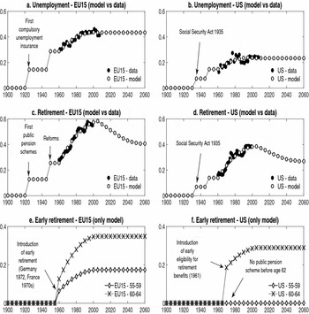
Figure B.1. Gross replacement rates (data and values in the model). The unemployment replacement rates (ρ u ) are shown in panels a and b, those for mandatory retirement (ρ r ) in panels c and d, and those for early retirement (ρ e ) in panels e and f. See Appendix B for details and Table 1 for the specific 2005 values.
(i) Unemployment benefits
Net replacement rates for the unemployed vary greatly with unemployment duration. They generally fall after the first year of an unemployment spell. In the EU15 in 2005, the net replacement rate during an unemployment spell fell from 55.02% in the first year to 22.88% in the fifth year [OECD (2009a), Table 1.6, population-weighted averages]. As unemployment duration is on average close to 1.5 years in EU15 countries, we set the 5-year (one period in our model) net unemployment benefit at 90% of the net replacement rates in the first year of an unemployment spell, i.e., 49.52%. Given the values for tax rates described in Section 5, the 2005 gross replacement rate over a 5-year unemployment spell is ρ u 2005 = (1 − τ w ) × 49.52% = 43.45% in the EU15. In the US, again in 2005, the net values were 28% in the first year of unemployment and zero from then on [OECD (2009a), Table 1.6, population-weighted averages]. As a result, the 5-year (one period in our model) net unemployment benefit should be only small. However, as unemployment duration is quite short in the US (between 3 and 4.5 months over the 2003–2007 period), we set this close to the replacement rate (at 90%) for the first year of unemployment. This produces a net 5-year replacement rate of 25.2% and, given the values of the tax rates described in Section 5, a 2005 gross replacement rate over a 5-year unemployment spell of ρ u 2005 = (1 − τ w ) × 25.2% = 23.27% in the US.
To calculate the gross replacement rates before 2005, we use historical movements normalized to match the ρ u 2005 values described above. In the EU15, (only) voluntary unemployment-benefit plans were established in a number of continental European cities between 1890 and World War I. The first national compulsory unemployment-insurance system of any country was established in Great Britain in 1911, followed by Italy 8 years later. Over the next decade, other European countries established such schemes, covering 35 million people by 1937 [Friedman (Reference Friedman1937)]. We thus set the EU15 replacement rate to zero from 1900 to 1920. From 1925 to 1945, the replacement rate was constant at one half of the value observed between 1950 and 1960. Social-welfare transfers rose afterwards, and especially rapidly in the 1960s and 1970s. The change in the (gross) unemployment-replacement rate over this 1960–2005 period is calculated from the OECD’s “summary measure of benefit entitlements,” a bi-annual database collected over the 1961–2007 period [see also Martin (Reference Martin1996)]. The OECD summary measure is defined as the average of the gross unemployment-benefit replacement rates for two earnings levels, three family situations and three unemployment durations. We use these data to create a second-order polynomial trend for the unemployment replacement rate.Footnote 22 We hold replacement rates constant after 2005. In the US, few states provided unemployment benefits on their own initiative before 1935, and only few workers were covered by such schemes [Friedman (Reference Friedman1937)]. For this reason, the US replacement rate is set to zero from 1900 to 1930. The federal government established the first nationwide unemployment-benefit scheme with the Social Security Act that was approved on the 14th of August 1935. By the end of 1936, 35 States had passed unemployment compensation laws covering about 18 million people. From 1935 to 1945, the replacement rate was constant and equal to half of the value observed between 1950 and 1960. It started to rise continuously from 1960 onwards, according to the trend calculated from the OECD data described above. We hold replacement rates constant after 2005. The top panels in Figure B.1 show these historical and predicted movements, and Table 1 displays the 2005 values.
(ii) Mandatory (normal) retirement benefits
We use the same method as above, fixing the 2005 values and normalizing historical and predicted movements around this period. The reference wage used to calculate pension benefits is typically an average over the best years of activity. We, therefore, set it to the average wage of workers of age 45–64 years. For a given replacement rate, our formulation implies that pensions are indexed to current wages. The values for the replacement rate correspond to the gross replacement rates by the level of individual earnings (mandatory pension programs) reported by the OECD (2009b). We have ρ r 2005 equal to 58.24% for the EU15 (population-weighted country average) and 38.6% for the US in 2005. Note that social-security systems are not only characterized by their generosity and size, but also by their degree of redistribution [Casamatta et al. (Reference Casamatta, Cremer and Pestieau2000)].
In the EU15, most countries introduced their first public pension scheme before or around World War I: Germany in 1889, France in 1910, Italy in 1919, Belgium in 1924, and Finland in 1937 [Ebbinghaus and Gronwald (Reference Ebbinghaus and Gronwald2011), Table 1]. The average year of the first pension scheme across the EU15 was 1920, and accordingly the replacement rate is set to zero from 1900 to 1915. The coverage of these first schemes was often limited to a certain type of worker (e.g., blue-collar workers in Germany). From 1920 to 1945, the pension replacement rate is assumed to be constant (as a result of the insecure interwar and World War II periods) at half of the 1950 value. Pension schemes evolved after World War II (being either reinforced or reformed). These changes started between 1945 (France, Belgium) and 1956 (Denmark, Finland, Netherlands), and so on average around 1950 [Ebbinghaus and Gronwald (Reference Ebbinghaus and Gronwald2011), Table 1]. The replacement rate is, therefore, higher from 1950 onwards. We assume it to be constant between 1950 and 1960, and thereafter to follow the trend calculated using the OECD data over the 1960–1999 period [Cornelisse and Goudswaard (Reference Cornelisse and Goudswaard2001), Annex 1]. A second-order polynomial trend is again used to trace out the evolution of mandatory retirement replacement rates over the 1950–2005 period. In the US, before 1935, old-age support was left to individual states, and most elderly relied on support from their extended family [Capretta (Reference Capretta2007)]. The Social Security Act in 1935 established the first national system of old-age benefits, which was designed to pay benefits to retired workers aged 65 years and over [Friedman (Reference Friedman1937)]. Coverage remained limited, however, and the pension benefit was modest [Capretta (Reference Capretta2007)]. From this evidence, we set the replacement rate to zero from 1900 to 1930, and from 1935 to 1945 to half of the rate between 1950 and 1960. According to Whitehouse et al. (Reference Whitehouse, D'Addio, Chomik and Reilly2009), there was a rapid growth in real pensions after 1960 [see also Blöndal and Scarpetta (Reference Blöndal and Scarpetta1998), Table III.3]. Between 1960 and 2005, the change in the replacement rates for normal retirement is approximated by the change in social benefits as a percentage of GDP, taken from the above mentioned OECD data in Cornelisse and Goudswaard (Reference Cornelisse and Goudswaard2001).
To restrict the rise in pension expenditures, a number of countries have recently undertaken significant reforms of their pay-as-you-go pension systems [see IMF (2010a), Appendices IV and V]. Our baseline scenario incorporates these reforms via progressive drops in the replacement rate from 2005 onwards: we assume, in both regions, a 20% fall in the replacement rate by 2030 and a 30% fall by 2055. With these changes in the pension replacement rates, the ratio of public-pension expenditure to GDP increases by similar magnitudes in our baseline as in official projections [European Commission (2009), IMF (2010b)]. Moreover, our model yields similar results to estimate that consider only the demographic effect on public-pension expenditures, i.e., without future changes in replacement rates [Bongaarts (Reference Bongaarts2004), European Commission (2009)]. These historical and projected data are plotted in the intermediate panels of Figure B.1. Table 1 shows the 2005 values.
(iii) Early-retirement benefits
We again use the same method, fixing the 2005 values and normalizing historical and predicted movements around this period. Calculating early-retirement replacement rates for a single European country and, in addition, a unique value for early-retirement benefits over the whole EU15, is not straightforward. In most countries, age 60 years is the first opportunity for early retirement. However, the effective early-retirement age is ambiguous, as some countries provide unemployment and disability programs allowing for early retirement for workers under 60 years [Gruber and Wise (Reference Gruber and Wise1999)]. For instance, in countries where such programs exist (e.g., Belgium, France, the Netherlands, and Germany), the departure rates from the labor force before the social-security early-retirement age are above 20%. This is, for example, the case for employees who are laid-off and eligible for large benefits before age 60 years. Additional complexity arises from the status classification system. In France, unemployed senior workers (over 60 years) receive social-security benefits and are classified as retired. In the Netherlands, the UK, Germany, and Sweden, senior workers receiving disability benefits start to receive social-security benefits at age 65 years and are only then classified as retired [Gruber and Wise (Reference Gruber and Wise1999), p.28]. Given this, the 2005 value for the gross replacement rate at age 60–64 years in the EU15 is based on OECD calculations [see Duval (Reference Duval2003)] and set to ρ e 7, 2005 = 34.90%. However, as not every EU country provides retirement benefits to those retiring before age 60 years, and not every senior worker qualifies for these programs, we set ρ e 6, 2005 = 0.5 × ρ e 7, 2005 [Gruber and Wise (Reference Gruber and Wise2004), p.15]. Note that, in the US, the hazard rates for not being in the labor force are close to zero before age 54 years, increase gradually between 54 and 61 years, and then jump sharply at the first year of early retirement (age 62 years). The low departure rates at ages 54–61 years come from eligibility for early retirement under employer provided pension plans rather than public-pension schemes. We therefore set the 2005 gross replacement rate for early retirement for workers aged 55–59 years to ρ e 6, 2005 = 0. In addition, workers retiring between age 62 years and the normal retirement age (NRA) face a reduction in their pension benefits (as a function of the time to NRA, and limited to benefits paid in the months before the NRA). In the US, the gross replacement rate for early retirement at ages 60–64 years is set to 75% of the benefit received at the NRA: ρ e 7, 2005 = 0.75 × ρ r 2005 = 28.95%.Footnote 23
Early retirement was introduced in 1972 in Germany and in the early 1970s in France [Gruber and Wise (Reference Gruber and Wise1999)]. Accordingly, in the EU15, the gross replacement rate for both 55–59 and 66–64-year olds is zero before 1970, that is ρ e 6, t = ρ e 7, t = 0. From 1970 onwards, these ages follow the same path as that of normal pension benefits, normalized to match the 2005 values mentioned above. More precisely, ρ e 7, t = ρ e 7, 2005 × ρ r t /ρ r 2005 and ρ e 6, t = ρ e 6, 2005 × ρ r t /ρ r 2005. In the US, early eligibility for retirement benefits was introduced in 1961 [Gruber and Wise (Reference Gruber and Wise1999)]. As a consequence, the replacement rate for early retirement is set to zero before 1960: ρ e 6, t = ρ e 7, t = 0. From 1960 onwards, this evolves in the same way as the normal pension benefit replacement rate: ρ e 7, t = ρ e 7, 2005 × ρ r t /ρ r 2005 and ρ e 6, t = ρ e 6, 2005 × ρ r t /ρ r 2005 = 0. These historical and projected data are plotted in the bottom panels of Figure B.1. Table 1 shows the 2005 values.
APPENDIX C: ADDITIONAL INFORMATION ON THE LABOR-MARKET PARAMETERS
This Appendix provides additional information on the calibration of the labor-market parameters. It first describes the calculation of the activity and early-retirement rate targets before explaining the calibration of the matching efficiency ν, worker bargaining power η, and vacancy-cost a parameters.
We first explain the calculation of the target values for the early-retirement and activity rates for the age classes 55–59 years, 60–64 years, and 55–64 years in Table 2. In our model, the age class can be split into P = A + E, where the A are employed and unemployed and the E are the early retired, while in the data P = A + E + N, where the N are those who do not participate in the labor market. Our model thus overestimates senior activity rates (A/(A + E)) compared to those in the data (A/(A + E + N)). We hence calculate the target values for senior-activity rates correcting for labor-market participation. The values of A and P come from the OECD (2010a), applying the following formula to calculate the senior-activity rates of the above three age classes: A/(P − N), with N = n P and n the proportion of inactive men. We calculate n using data for 45–49-year old men over the 2003–2007 period (we can assume that there are no early retired among the inactive individuals in this age class, but similar senior activity rates are obtained using inactive men in the age classes 40–44 years and 25–54 years). Last, the early-retirement rate of individuals aged 55–59 years in 2005 (λ55 − 59) is calculated from OECD (2010a) data as the difference between the employed and unemployed aged 55–59 years in the 2003–2007 period (yearly average) and employed and unemployed men aged 50–54 years in the 2000–2002 period (yearly average), divided by the size of the age class in 2003–2007. The early-retirement rate of individuals aged 60–64 years is calculated in a similar way.
The matching function (45), and the wage equation (36), and its associated matching elasticity and bargaining-power parameters, are two key elements of the search and matching set-up. We here further discuss the empirical viability of our calibration.
The most comprehensive survey of the matching function is probably Petrongolo and Pissarides (Reference Petrongolo and Pissarides2001). They show that most work that estimates aggregate matching functions finds constant returns to scale. That is, if the elasticity with respect to unemployment in the matching function is η U and that with respect to vacancies is η V , we must have η U + η V = 1. Also, the estimates of the elasticities η V = 1 − η U vary greatly according to the approach and the data. Petrongolo and Pissarides (Reference Petrongolo and Pissarides2001) suggest a plausible empirical range for the elasticity on vacancies of 0.3 to 0.5. More recently, using only US labor-market data, Shimer (Reference Shimer2005) finds an elasticity of 0.3 when regressing the job-finding probability on tightness, Mortensen and Nagypal (Reference Mortensen and Nagypal2007) infer a value of 0.5 from the slope of the Beveridge curve, and Borrowczyk-Martins et al. (Reference Borrowczyk-Martins, Jolivet and Postel-Vinay2013) suggest an elasticity of 0.7 via an estimation method that avoids the endogeneity bias in search behavior. In the dynamic stochastic general equilibrium (DSGE) literature, Gertler et al. (Reference Gertler, Sala and Trigari2008) construct a model with search unemployment for the US and calibrate the elasticity parameter to 0.5. Christoffel et al. (Reference Christoffel, Kuester and Linzert2009b) provide a similar model for the Euro area, and estimate the same parameter to be 0.33. Our matching function yields an elasticity η V = 1/(1 + (V t /Ω t )ν) < 1 and an elasticity η U = (V t /Ω t )ν/(1 + (V t /Ω t )ν) < 1. We first note that η U + η V = 1 so that our function conforms to the constant returns to scale suggested by the empirical data. Second, we note that, contrary to – for example – a Cobb–Douglas specification, our elasticities change over time and depend on labor-market tightness V t /Ω t . Our calibration implies that η V = 0.63 in the EU15 and η V = 0.40 in the US in 2005. These figures are in the range of admissible values mentioned above. Note that η U − 1 measures the negative externality (congestion) caused by the unemployed on the other unemployed [see Petrongolo and Pissarides (Reference Petrongolo and Pissarides2001) for a discussion]. Our calibration suggests that there is more congestion in the EU15 than in the US in 2005.
Worker bargaining power η is another important parameter in the search and matching framework. A number of empirical contributions have tried to quantify this parameter on a 0 to 1 scale. For example, Abowd and Allain (Reference Abowd and Allain1996) estimate a bargaining power figure of 0.4 in French worker-firm panel data. Crépon et al. (Reference Crépon, Desplatz and Mairesse2010) estimate η = 0.6 in a panel of French manufacturing firms using the Generalized Method of Moments. They also show that not taking labor-market imperfections into account underestimates the firm rent captured by workers. More recently, Dumont et al. (Reference Dumont, Rayp and Willemé2012) distinguish between low- and high-skilled workers in Belgian firm data and show that the average – across industries – bargaining power of the low-skilled is around 0.6, whereas that of the high-skilled is 0.55. The survey of Mortensen and Nagypal (Reference Mortensen and Nagypal2007) proposes a value of 0.5, which therefore seems to be a conventional finding in the empirical literature. This is also the value often found in calibrated models, as for instance in the seminal paper of Mortensen and Pissarides (Reference Mortensen and Pissarides1994) or in more recent monetary DSGE papers with search and matching, like Christoffel et al. (Reference Christoffel, Kuester and Linzert2009b). Alternatively, worker bargaining power in simpler DSGE models is often set equal to the elasticity of the matching function with respect to unemployment in order to satisfy the so-called Hosios condition (the equivalence between the decentralized and centralized equilibria). For instance, in their real business cycle models with search and matching, Merz (Reference Merz1995) and Andolfatto (Reference Andolfatto1996) set bargaining power to 0.4 as they both use the calibration η U = 1 − η V = 0.4. We here set worker bargaining power η to the conventional value of 0.5. We moreover observe that η approximately corresponds to the mean of our matching elasticities to unemployment in the EU15 (η U = 1 − η V = 0.37) and the US (η U = 1 − η V = 0.60).
The vacancy-cost parameter a is not directly inferred from data or empirical analysis but is instead set to target specific values. As a result, we obtain a lower vacancy cost in the EU than in the US. The mathematical intuition for this result comes from a simplified (one-generation) job-creation curve
 $\mathsf{a}/q=h\,A\,F_H-(1+\tau ^f)w$
. We know from the data (see Table 1) that τ
f
is three times higher in Europe than in the US. This means that, all else equal, we obtain a much lower value of a with the EU calibration than with the US calibration. A lower a is therefore a side effect of higher labor-income taxation in Europe.
$\mathsf{a}/q=h\,A\,F_H-(1+\tau ^f)w$
. We know from the data (see Table 1) that τ
f
is three times higher in Europe than in the US. This means that, all else equal, we obtain a much lower value of a with the EU calibration than with the US calibration. A lower a is therefore a side effect of higher labor-income taxation in Europe.
APPENDIX D: THE SEPARATE EFFECTS OF FERTILITY AND LONGEVITY
There are three types of demographic variables in the model: fertility (x t ), longevity (θ a, t ), and migration (X a, t ). This section briefly describes the separate effects of fertility and longevity. It is worth noting that “fertility” here refers to the growth rate of the first generation (as is usual in this kind of model), which is here the 25–29 years age class (fertility thus includes not only the postponed effects of reproduction of the population aged under 30 years but also migration by those under 30 years).
Figure D.1 shows how population changes in both regions (the “LMIDO” lines); it also plots the same lines when holding fertility constant after 1955 (LMIDO (cst fertility)) and holding longevity constant (LMIDO (cst longevity)). Note first that between 1960 and 2010, the EU15 population (25+ years) rose by 50% while that in the US doubled. In the EU15, fertility and longevity have had similar impacts on population change, as population movements are similar when either component is kept constant after 1955 (in both cases, population rises by about 30% between 1960 and 2010). In the US, however, fertility is significantly more important than longevity in explaining the rise in population (which grows by 90% when longevity is constant and 30% when fertility is kept constant).

Figure D.1. Population 25+ years (baseline vs. constant fertility vs. constant longevity). Population 25+ years in millions. LMIDO refers to the model with demographic and labor-market institution changes and perfect international-capital mobility. In LMIDO (cst fertility), fertility (x t ) is kept constant after 1955 to highlight the effects of longevity, and in LMIDO (cst longevity), longevity (θ a, t + a ) is constant after 1955 to highlight the effects of fertility. Note that “fertility” here refers to the growth rate of the first generation of the model (the 25–29-year olds).
Figure D.2 (panels a and b) shows that lower fertility (the “LMIDO (cst fertility)” lines) leads to lower unemployment rates, but reduced longevity (LMIDO (cst longevity)) to higher unemployment (see also Proposition 1 in Section 3.1). Lower fertility implies more capital per worker, while lower life expectancy induces lower savings and thus less capital per worker. Finally, panel c of Figure D.2 indicates that longevity has had a favorable impact on the unemployment gap from the point of view of the EU15 (without any change in longevity the gap would have been higher) as did fertility up to 1990. After 1990, the absence of any change in fertility would have led to a lower EU15–US gap.

Figure D.2. The effects of fertility and longevity on the unemployment rates and gap. Unemployment rates are expressed in percent. LMIDO refers to the model with demographic and labor-market institution changes and perfect international capital mobility. In LMIDO (cst fertility) fertility (x t ) is kept constant after 1955 to highlight the effects of longevity, and in LMIDO (cst longevity) longevity (θ a, t + a ) is constant after 1955 to highlight the effects of fertility. Note that “fertility” here refers to the growth rate of the first generation of the model (the 25–29-year olds).
APPENDIX E: TAXES
Consumption taxes
We assume that consumption tax rates change each period so as to balance the government’s budget. These adjustments affect the total (labor + consumption) tax wedge without changing the gross or net replacement rates. Figure E.1 depicts the evolution of consumption taxes in the LMIDO model. As expected, the consumption tax rate rises more in the EU than in the US. Changes in the generosity of the welfare state (exogenous changes in gross replacement rates) and/or endogenous changes in the unemployment rate bring about changes in social-security expenditures that are matched by movements in the consumption tax. Most of the tax increase takes place between 1965 and 1995. Over that period, the differential between the EU and the US increases by 5.6 pp and implies a similar increase in the total tax-wedge differential, a figure that is compatible with the values in Mendoza et al. (Reference Mendoza, Razin and Tesar1994).

Figure E.1. Evolution of consumption tax rates (in percent) in the LMIDO model.
Capital-income taxes
As noted in Section 6.3, we chose not to model the impact of changes in corporate and personal capital-income taxes. Introducing corporate capital-income taxes changes the worldwide no-arbitrage condition, as shown in equation (48), where τ x t denotes the marginal tax rate on corporate profits, net of capital depreciation. In this setup, asymmetric corporate-income taxation is bound to have considerable effects on investment location choices and capital flows. A one pp lower US corporate tax rate, for instance, has the same effect as an exogenous one pp rise in US total factor productivity. This result depends crucially, of course, on the assumption of perfect capital mobility, no transportation costs and no trade barriers. Excess savings in one country are thus channeled to the other until interest rates and marginal capital productivity are equalized. These reallocations of capital are matched by flows of goods in the opposite direction. This is again a simplification. In actual economies, the choice of investment location will be affected by agglomeration advantages, the size of the respective domestic goods markets, transportation costs, and so on. Such factors reduce the volatility and size of international capital flows. They also help explain why the estimated effects of tax wedges on capital flows are much smaller than those predicted in standard neoclassical models [see, for instance, Hajkova et al. (Reference Hajkova, Nicoletti, Vartia and Yoo2006)] and may explain why countries with large domestic markets may benefit from sizeable international capital inflows despite having relatively high tax rates. In this context, Devereux and Griffith (Reference Devereux and Griffith1998) find that effective tax rates do not play a significant role in the decision of US multinationals to locate in Europe, although they do affect the choice of where to locate within Europe.
It is also quite hard to summarize the consequences of actual corporate-tax systems in a single number. Statutory rates fell in many countries after 1985, including the US, France, Germany, and many EU countries (apart from Italy). As tax bases have at the same time widened, the fall in the effective marginal tax rate is much less pronounced and starts much later, in the late 1990s [except in Germany, see Devereux (Reference Devereux2007)]. The interactions between different tax systems, together with firms’ tax-planning activities, can significantly reduce the actual tax wedge between countries and contribute to the difficulty of correctly assessing the actual taxation rate firms face in a given country. In this context, Backus et al. (Reference Backus, Henriksen and Storesletten2008) stress the contrast between tax measures based on official tax rates and those based on actual tax revenues, as developed by Mendoza et al. (Reference Mendoza, Razin and Tesar1994). The two measures are illustrated in Figure E.2. The right-hand panel plots the evolution of statutory rates (source: OECD, statutory central government non-targeted corporate-income tax rate); the left-hand panel (labeled in percent of GOS) plots the evolution of corporate income-tax revenues in pp of the gross operating surplus of corporations (source: OECD, revenue statistics and national accounts, detailed tables). We clearly see that the trend in the EU-US corporate-tax differential depends on the measure used: the trend is negative with statutory taxes but positive with tax revenues.

Figure E.2. Historical evolutions of corporate-income taxes (CIT). Sources. Panel a: OECD, revenue statistics, and national accounts, detailed tables. The EU revenue-based tax rate is a weighted average over three countries (FR, DE, and NL). The tax is labeled in percentage of gross operating surplus (GOS). Panel b: OECD, statutory central government non-targeted corporate-income tax rate. The EU statutory rate is calculated as a weighted average over six countries: BE, FR, DE, IT, NL, and ES.
Introducing all of these elements explicitly is beyond the scope of our paper. However, it is useful to test the robustness of our unemployment-gap model by checking how sensitive the results are to the size of capital flows and the assumption of perfect capital mobility. We thus introduce imperfect capital mobility, so as to match observed capital flows. The impact of this change on the estimated unemployment gap is discussed in Section 6.2. Imperfect capital mobility reduces capital flows, but has only a small effect on the unemployment gap.


