1. INTRODUCTION
Even in an age of instant communication and rapid transportation, immigration to a new country is a risky endeavor. Migrants face significant legal barriers, cultural adjustment costs, financial burdens, and numerous uncertainties while they try to reach and settle in their destination. By providing financial, legal, and social support, existing personal networks increase the benefits and lower the costs of immigration faced by new migrants. As a result, migration flows generate diaspora networks and networks, in turn, enhance migration flows. This process might lead to an acceleration of migration even when economic disparities leading push and pull forces between countries remain stable. The main objective of this paper is to identify and quantify the relative importance of two main channels through which migrant networks influence migration patterns.
The first channel, referred to the assimilation channel operates through the lowering of private costs which generally matter after the migrant crosses the border. These private costs cover a wide range of hurdles faced by the migrants in finding employment, deciphering foreign cultural norms, and adjusting to a new linguistic and social environment. All of these obstacles tend to be local in nature and the support provided by the existing local network can be crucial. One of the earliest papers, Massey et al. (Reference Massey, Arango, Hugo, Kouaouci, Pellegrino and Taylor1993) show how diasporas reduce moving costs, both at the community level (people from the same origin country forming local communities), and at the family level (friends and relatives). Such networks provide information and assistance to new migrants before they leave and after they arrive. This process facilitates newcomers’ integration in the destination economy, reduces uncertainty, and increases the expected benefits from migration. Based on a sample of individuals originating from multiple communities in Mexico and residing in the US, Munshi (Reference Munshi2003) shows that a new migrant is more likely to be employed and earn higher wage when his/her network is larger.
The second channel, policy channel, is the overcoming of legal entry barriers imposed by the destination country. Members of the diaspora network help the new migrant at the border before she/he arrives at the final destination. More specifically, former migrants who have already acquired citizenship or certain residency rights in the destination countries become eligible to sponsor members of their families and other relatives. Family reunification programs are the main routes for many potential migrants in most countries of the Organization for Economic Cooperation and Development (hereafter OECD).Footnote 1
Migration literature recognizes the critical role of diaspora networks in determining the size, skill structure, and destination composition of migrant flows.Footnote 2 Even though the two rather distinct roles of diasporas (lowering of assimilation costs and overcoming policy induced legal barriers) are recognized in the literature, there has been no attempts to empirically assess their relative importance. An ideal approach for this goal would be to directly use micro data on personal characteristics and the specific entry paths migrants choose. Appropriate use of indicators on migration policies along with diaspora characteristics could provide information on the relative importance of family-based admission of new migrants. For example, the New Immigrant Survey (NIS) provides data on various entry tracks migrants from different countries of origin use. Unfortunately, for many origin countries, the number of observations in the NIS is rather small. Official data from the Immigration and Naturalization Service are richer and allow measuring sponsorship rates and migration multipliers (Jaeger, Reference Jaeger2007).
In our context, the use of micro data is subject to certain limitations. First, sponsorship rates and migration multipliers are the outcomes of the two forces that we aim to disentangle, i.e. (i) the willingness of potential migrants to be sponsored and apply for a residency permit, and (ii) the probability to be granted the residency after applying. Second, information on changes in immigration laws might not be enough to gauge the importance of family reunification policies over time. For example, many undocumented migrants became legal residents after amnesty programs implemented in the US in the 1990s. Those regularized migrants, in turn, became eligible to bring their close relatives to the US over the following decade. This process results in a rapid increase in the number of migrants coming through family reunification programs in spite of no significant change in the US migration laws. Another issue is that a significant number of highly skilled immigrants to the US used family-based tracks for convenience while they were fully eligible to use economic migration tracks such as H1B or special talent visas. Ascribing their migration pattern only to the family reunification track would give a distorted picture of the importance of each migration channel.
As an alternative to the use of individual data on immigration paths, this paper develops a different identification strategy using aggregate/macro data available at the metropolitan area (referred to as “city” for simplicity in the remainder of the paper) level for the United States.Footnote 3 As mentioned earlier, the role of the diasporas in overcoming legal entry barriers operates at the border before the migrant settles in a given city. Thus, the probability for a migrant to obtain legal entry and residence permit through a family reunification program depends on the total size of the network already present in the United States, not necessarily on the distribution of this diaspora across different cities.
The assimilation effect, on the other hand, is predominantly local and matters after the migrant chooses a city to settle. Indeed, in the network theory, social links are formed by individuals who trade off the costs and potential rewards of creating a network (Genicot and Ray, Reference Genicot and Ray2003; Jackson and Rogers, Reference Jackson and Rogers2007). The main benefits from migration networks include material support and transfer of information on the local provision of public goods, the housing market, access to credit, labor or production opportunities, and mutual help (Comola and Mendola, Reference Comola and Mendola2015). Existing literature has shown that the net benefits of the network decrease with the geographic distance between network members and newcomers (Massey and Espinosa, Reference Massey and Espinosa1997; Massey et al., Reference Massey, Alarcon, Durand and Gonzalez1987; Fafchamps and Gubert, Reference Fafchamps and Gubert2007; Mayer and Puller, Reference Mayer and Puller2008; Fafchamps et al., Reference Fafchamps, Goyal and van der Leij2010). Interpersonal links are more likely to be formed between geographically and socially proximate individuals rather than distant fellows. The recent literature adopts a dyadic approach (Comola and Mendola, Reference Comola and Mendola2015; Giuletti, Wahba and Zenou, Reference Giuletti, Wahba and Zenou2014) and documents how the main assimilation effects – namely housing and labor market benefits – require that the network has a strong local presence relative to the migrants. For example, if a migrant lives in Chicago, the diaspora in Los Angeles is unlikely to be of much help to him in terms of finding a job, an apartment or a school for his children, especially relative to the network in Chicago. This is the distinction we exploit to identify the relative importance of the two channels. Obviously, we cannot assure that assimilation effects are purely local, i.e. network members might still assist with the assimilation of new migrants from a distance. Using US metropolitan areas as our main locations, we hypothesize that such non-local assimilation effects are small. Nevertheless, we acknowledge that our method ignores potential non-local assimilation externalities and might over-estimate the magnitude of the policy channel. Our estimates for the latter channel may be considered as an upper bound.
We first show that the overall network effect is strong. On average, each settled immigrant present in the United States in 1990 (resp. in 1980) attracted 0.97 (resp. 0.83) additional migrants within the following decade. These elasticities are in the same order of magnitude as Bin (Reference Bin2007) and Beine et al. (Reference Beine, Docquier and Ozden2011).Footnote 4 In an earlier analysis, Jasso and Rosenzweig (Reference Jasso and Rosenzweig1989) find a sponsorship rate ranging between 0.3 and 0.7 after one decade for the 1971 cohort of US immigrants (and an average migration multiplier of 1.2 in the long-run). We obtain slightly greater effects as the US family reunification program becomes more generous over time.
Our second and more important contribution is the dissection of the network effect into the private assimilation and legal components. As mentioned above, observed sponsorship rates reflect the joint effect of networks on migration aspirations and realization rates. Over the 1990s, the decrease in assimilation costs induced by the presence of a migrant explains the entry of 0.7 additional migrants; the decrease in legal costs explains the entry of 0.3 additional immigrants. Despite the fact that our assessment of the policy channel can be taken as an upper bound, this channel accounts for only a quarter of the total network elasticity; the rest is due to the assimilation effect. Furthermore, the effect is smaller for college graduates than for the less educated.Footnote 5 These results are strongly robust to sample selection, identification assumptions, treatment for unobserved bilateral heterogeneity, and endogeneity of the network. In addition, we find that the estimated policy externality was higher in the 1990s than in the 1980s. This can be easily explained by the fact that family reunification programs became more generous in the 1990s with the implementation of the 1986 Immigration Reform and Control Act, and 1990 US Immigration Act. Over the 1980s, the legal channel was smaller (lower than 0.1) whereas the assimilation elasticity is remarkably stable. This is consistent with our presumptions that assimilation externalities are mainly local and independent of policy reforms, suggesting that the non-local externality predominantly pertains to the legal channel. These results are robust to the specification, to the choice of the dependent variable, and to the definition of the relevant network.
Our results have certain policy implications. Over the last several decades, the impact of government policies on shaping migration patterns has become a central policy issue. The main channel through which governments can impact the size of the migration flows would be through the generosity of the family reunification programs. As we discuss in the next section, a majority of legal entries (and around 40 percent of all entries when undocumented migrants are taken into account) into the United States takes place through this channel. However, our results indicate that even complete elimination of family reunification programs would not eliminate the impact of disaporas in attracting future migration inflows. In other words, government’s capacity to curb the diaspora multiplier exists, but is somewhat limited.
The paper proceeds in the following order. In Section 2, we develop a simple theoretical model showing that, under functional homogeneity of the two network externalities, these two different channels can be identified using bilateral data by country of origin of migrants and by metropolitan area of destination (see Section 3). In Section 4, we test our model using US data covering the 1980–2000 period and provide many robustness checks based on educational differences (in Section 4.2), time dimension (in Section 4.3), alternative migrant definitions or geographic areas (see Sections 4.4 and 4.5), and control for potential sources of endogeneity (see Section 4.7). Finally, Section 5 concludes.
2. MICROFOUNDATIONS
We use a random utility model of labor migration where individuals with heterogeneous skill types s (s = 1, …, S) born in origin country i (i = 1, …, I) decide whether to stay in their home country i or emigrate to location (or city) j (j = 1, …, J) in the destination country. In the estimation, the set of locations are different cities in a single destination country, the US. These locations share the same national immigration policy but they differ in other local attributes. As emphasized by Grogger and Hanson (Reference Grogger and Hanson2011), we assume the individual utility is linear in income and includes possible migration and assimilation costs as well as characteristics of the city of residence.
The utility of a type-s individual born in country i and staying in his home country i is given by
 $$\begin{equation*}
U_{ii}^{s}=w_{i}^{s}+A_{i}^{s}+\varepsilon _{ii}^{s},
\end{equation*}$$
$$\begin{equation*}
U_{ii}^{s}=w_{i}^{s}+A_{i}^{s}+\varepsilon _{ii}^{s},
\end{equation*}$$where wsi denotes the expected labor income in location i, Ai denotes country i’s characteristics (amenities, public expenditures, climate, etc.), and εsii is a random utility component.
The utility obtained when the same person migrates to location j is given by
 $$\begin{equation*}
U_{ij}^{s}=w_{j}^{s}+A_{j}^{s}-C_{ij}^{s}-V_{i}^{s}+\varepsilon _{ij}^{s},
\end{equation*}$$]></tex-math>
</alternatives>
</disp-formula>
where <italic>w<sup>s</sup><sub>j</sub></italic>, <italic>A<sup>s</sup><sub>j</sub></italic>, and ε<sup><italic>s</italic></sup><sub><italic>ij</italic></sub> denote the same variables as above. The deterministic component of utility, <italic>w<sup>s</sup><sub>j</sub></italic> + <italic>A<sub>j</sub></italic><sup><italic>s</italic></sup>, shapes the mean level of utility that a native from country <italic>i</italic> can reach in destination country <italic>j</italic> or in her home country <italic>i</italic> (if he were to stay home). In addition, two types of migration costs are presented. First, cost element, <italic>C<sup>s</sup><sub>ij</sub></italic> captures the mean level of moving and assimilation costs that are borne by the migrant when he moves from home country <italic>i</italic> to city <italic>j</italic>. When combined with (<italic>w<sup>s</sup><sub>j</sub></italic> + <italic>A<sub>j</sub></italic><sup><italic>s</italic></sup>) − (<italic>w<sup>s</sup><sub>i</sub></italic> + <italic>A<sub>i</sub></italic><sup><italic>s</italic></sup>), the assimilation cost <italic>C<sup>s</sup><sub>ij</sub></italic>, would determine the net benefit of migration into different destinations if there were no policy restrictions on labor mobility. In line with previous studies on network externalities (Hatton and Williamson, <xref ref-type="bibr" rid="ref020">2005</xref>; Pedersen et al., <xref ref-type="bibr" rid="ref037">2008</xref>; Beine et al., <xref ref-type="bibr" rid="ref002">2011</xref>; Giuletti et al., <xref ref-type="bibr" rid="ref018">2014</xref>), we assume below that <italic>C<sup>s</sup><sub>ij</sub></italic> depends on the network size in location <italic>j</italic> since this local network size directly affects the probability that an immigrant from country <italic>i</italic> has a community member, friend, or relative in location <italic>j</italic>. Upon arrival, local network members may facilitate easier adaptation of newcomers into their new environment. Prior to arrival, they may share information with potential migrants and reduce search costs. The network outside <italic>j</italic>, on the other hand, has no effect on the assimilation costs of migrants moving to <italic>j</italic>.</p>
<p>The second cost element, <italic>V<sup>s</sup><sub>i</sub></italic> represents the mean level of policy induced costs borne by the migrant to overcome the legal hurdles set by the destination country’s government’s (policy channel). Since family reunification programs are implemented at the national level, <italic>V<sup>s</sup><sub>i</sub></italic> depends on the network size at the country level, not at the city level. This is the reason for the absence of subscript <italic>j</italic> in <italic>V<sup>s</sup><sub>i</sub></italic>. The national network size directly affects the probability that a potential migrant has a relative in the US and becomes eligible for the family reunification program. Again, the random component, ε<sup><italic>s</italic></sup><sub><italic>ij</italic></sub>, captures individual heterogeneity in utility within a skill group due to occupational characteristics, abilities, preferences, etc. Heterogeneity may also be caused by the fact that not all migrants from country <italic>i</italic> have a family member or friend in the destination country, or by the fact that some migrants do not need to use family reunification visas as they might be eligible for employment or other visas.</p>
<p>We slightly abuse the terminology for simplification, and refer to <italic>C<sup>s</sup><sub>ij</sub></italic> as <italic>local assimilation costs</italic> and to <italic>V<sup>s</sup><sub>i</sub></italic> as <italic>national policy costs</italic>. Our key motivation to differentiate between these two types of costs is to gauge the capacity of the government to control the level of the immigration multiplier and influence future immigration flows. It is worth noting that we allow both of these costs to vary with skill type. High-skill workers are better informed than the low skilled, have higher capacity to assimilate or have more transferrable linguistic, technical, and cultural skills. In short, high skilled workers face lower assimilation costs. Finally, the skill type will affect visa or legal entry costs if there are selective immigration programs (such as the point-system in Canada or the H1-B program in the US) that specifically target highly educated workers and grant them various preferences.</p>
<p>The random term ε<sup><italic>s</italic></sup><sub><italic>ij</italic></sub> is assumed to follow an iid extreme-value distribution. Bertoli and Fernandez-Huertas Moraga (<xref ref-type="bibr" rid="ref004">2013</xref>, <xref ref-type="bibr" rid="ref005">2015</xref>) or Ortega and Peri (<xref ref-type="bibr" rid="ref036">2013</xref>) use more general distributions, allowing for a positive correlation in the realization of the shock across similar countries. In the empirical literature, generalizing the distribution of the random term is helpful to derive micro-founded gravity models accounting for multilateral resistance to migration. Augmenting the standard gravity model with appropriate fixed effects or correction terms improves the estimation of some key parameters. However, Bertoli and Fernandez-Huertas Moraga (<xref ref-type="bibr" rid="ref005">2015</xref>) show the estimated coefficient of the network effect is not significantly affected by the inclusion of these correction terms.</p>
<p>Let <italic>N<sup>s</sup><sub>i</sub></italic> denote the size of the native population of skill <italic>s</italic> that is within migration age in country <italic>i</italic>. When ε<sup><italic>s</italic></sup><sub><italic>ij</italic></sub> follows an iid extreme-value distribution, we can apply the results in McFadden (<xref ref-type="bibr" rid="ref032">1984</xref>) to write the probability that a type-<italic>s</italic> individual born in country <italic>i</italic> moves to location <italic>j</italic> as
<disp-formula>
<alternatives>
<graphic xmlns:xlink="http://www.w3.org/1999/xlink" xlink:href="S2054089215000139_eqnU3" xlink:type="simple" mime-subtype="gif"/>
<tex-math><![CDATA[$$\begin{equation*}
\Pr \big[ U_{ij}^{s}=\max\limits_{k}U_{ik}^{s}\big] =\frac{N_{ij}^{s} }{N_{i}^{s}}=\frac{\exp \big[ w_{j}^{s}+A_{j}^{s}-C_{ij}^{s}-V_{i}^{s} \big] }{\sum _{k}\exp \left[ w_{k}^{s}+A_{k}^{s}-C_{ik}^{s}-V_{i}^{s}\right] },\end{equation*}$$
$$\begin{equation*}
U_{ij}^{s}=w_{j}^{s}+A_{j}^{s}-C_{ij}^{s}-V_{i}^{s}+\varepsilon _{ij}^{s},
\end{equation*}$$]></tex-math>
</alternatives>
</disp-formula>
where <italic>w<sup>s</sup><sub>j</sub></italic>, <italic>A<sup>s</sup><sub>j</sub></italic>, and ε<sup><italic>s</italic></sup><sub><italic>ij</italic></sub> denote the same variables as above. The deterministic component of utility, <italic>w<sup>s</sup><sub>j</sub></italic> + <italic>A<sub>j</sub></italic><sup><italic>s</italic></sup>, shapes the mean level of utility that a native from country <italic>i</italic> can reach in destination country <italic>j</italic> or in her home country <italic>i</italic> (if he were to stay home). In addition, two types of migration costs are presented. First, cost element, <italic>C<sup>s</sup><sub>ij</sub></italic> captures the mean level of moving and assimilation costs that are borne by the migrant when he moves from home country <italic>i</italic> to city <italic>j</italic>. When combined with (<italic>w<sup>s</sup><sub>j</sub></italic> + <italic>A<sub>j</sub></italic><sup><italic>s</italic></sup>) − (<italic>w<sup>s</sup><sub>i</sub></italic> + <italic>A<sub>i</sub></italic><sup><italic>s</italic></sup>), the assimilation cost <italic>C<sup>s</sup><sub>ij</sub></italic>, would determine the net benefit of migration into different destinations if there were no policy restrictions on labor mobility. In line with previous studies on network externalities (Hatton and Williamson, <xref ref-type="bibr" rid="ref020">2005</xref>; Pedersen et al., <xref ref-type="bibr" rid="ref037">2008</xref>; Beine et al., <xref ref-type="bibr" rid="ref002">2011</xref>; Giuletti et al., <xref ref-type="bibr" rid="ref018">2014</xref>), we assume below that <italic>C<sup>s</sup><sub>ij</sub></italic> depends on the network size in location <italic>j</italic> since this local network size directly affects the probability that an immigrant from country <italic>i</italic> has a community member, friend, or relative in location <italic>j</italic>. Upon arrival, local network members may facilitate easier adaptation of newcomers into their new environment. Prior to arrival, they may share information with potential migrants and reduce search costs. The network outside <italic>j</italic>, on the other hand, has no effect on the assimilation costs of migrants moving to <italic>j</italic>.</p>
<p>The second cost element, <italic>V<sup>s</sup><sub>i</sub></italic> represents the mean level of policy induced costs borne by the migrant to overcome the legal hurdles set by the destination country’s government’s (policy channel). Since family reunification programs are implemented at the national level, <italic>V<sup>s</sup><sub>i</sub></italic> depends on the network size at the country level, not at the city level. This is the reason for the absence of subscript <italic>j</italic> in <italic>V<sup>s</sup><sub>i</sub></italic>. The national network size directly affects the probability that a potential migrant has a relative in the US and becomes eligible for the family reunification program. Again, the random component, ε<sup><italic>s</italic></sup><sub><italic>ij</italic></sub>, captures individual heterogeneity in utility within a skill group due to occupational characteristics, abilities, preferences, etc. Heterogeneity may also be caused by the fact that not all migrants from country <italic>i</italic> have a family member or friend in the destination country, or by the fact that some migrants do not need to use family reunification visas as they might be eligible for employment or other visas.</p>
<p>We slightly abuse the terminology for simplification, and refer to <italic>C<sup>s</sup><sub>ij</sub></italic> as <italic>local assimilation costs</italic> and to <italic>V<sup>s</sup><sub>i</sub></italic> as <italic>national policy costs</italic>. Our key motivation to differentiate between these two types of costs is to gauge the capacity of the government to control the level of the immigration multiplier and influence future immigration flows. It is worth noting that we allow both of these costs to vary with skill type. High-skill workers are better informed than the low skilled, have higher capacity to assimilate or have more transferrable linguistic, technical, and cultural skills. In short, high skilled workers face lower assimilation costs. Finally, the skill type will affect visa or legal entry costs if there are selective immigration programs (such as the point-system in Canada or the H1-B program in the US) that specifically target highly educated workers and grant them various preferences.</p>
<p>The random term ε<sup><italic>s</italic></sup><sub><italic>ij</italic></sub> is assumed to follow an iid extreme-value distribution. Bertoli and Fernandez-Huertas Moraga (<xref ref-type="bibr" rid="ref004">2013</xref>, <xref ref-type="bibr" rid="ref005">2015</xref>) or Ortega and Peri (<xref ref-type="bibr" rid="ref036">2013</xref>) use more general distributions, allowing for a positive correlation in the realization of the shock across similar countries. In the empirical literature, generalizing the distribution of the random term is helpful to derive micro-founded gravity models accounting for multilateral resistance to migration. Augmenting the standard gravity model with appropriate fixed effects or correction terms improves the estimation of some key parameters. However, Bertoli and Fernandez-Huertas Moraga (<xref ref-type="bibr" rid="ref005">2015</xref>) show the estimated coefficient of the network effect is not significantly affected by the inclusion of these correction terms.</p>
<p>Let <italic>N<sup>s</sup><sub>i</sub></italic> denote the size of the native population of skill <italic>s</italic> that is within migration age in country <italic>i</italic>. When ε<sup><italic>s</italic></sup><sub><italic>ij</italic></sub> follows an iid extreme-value distribution, we can apply the results in McFadden (<xref ref-type="bibr" rid="ref032">1984</xref>) to write the probability that a type-<italic>s</italic> individual born in country <italic>i</italic> moves to location <italic>j</italic> as
<disp-formula>
<alternatives>
<graphic xmlns:xlink="http://www.w3.org/1999/xlink" xlink:href="S2054089215000139_eqnU3" xlink:type="simple" mime-subtype="gif"/>
<tex-math><![CDATA[$$\begin{equation*}
\Pr \big[ U_{ij}^{s}=\max\limits_{k}U_{ik}^{s}\big] =\frac{N_{ij}^{s} }{N_{i}^{s}}=\frac{\exp \big[ w_{j}^{s}+A_{j}^{s}-C_{ij}^{s}-V_{i}^{s} \big] }{\sum _{k}\exp \left[ w_{k}^{s}+A_{k}^{s}-C_{ik}^{s}-V_{i}^{s}\right] },\end{equation*}$$and the bilateral ratio of migrants in city j to the non-migrants is given by
 $$\begin{equation*}
\frac{N_{ij}^{s}}{N_{ii}^{s}}=\frac{\exp \big[ w_{j}^{s}+A_{j}^{s}-C_{ij}^{s}-V_{i}^{s}\big] }{\exp \left[ w_{i}^{s}+A_{i}^{s}\right]}.\end{equation*}$$
$$\begin{equation*}
\frac{N_{ij}^{s}}{N_{ii}^{s}}=\frac{\exp \big[ w_{j}^{s}+A_{j}^{s}-C_{ij}^{s}-V_{i}^{s}\big] }{\exp \left[ w_{i}^{s}+A_{i}^{s}\right]}.\end{equation*}$$Hence, the log ratio of emigrants in city j to residents of i (Nsij/Nii s) is given by the following expression:
 $$\begin{equation}
\ln \left[ \frac{N_{ij}^{s}}{N_{ii}^{s}}\right] =\left( w_{j}^{s}-w_{i}^{s}\right) +\left( A_{j}^{s}-A_{i}^{s}\right) -\left( C_{ij}^{s}+V_{i}^{s}\right).
\end{equation}$$
$$\begin{equation}
\ln \left[ \frac{N_{ij}^{s}}{N_{ii}^{s}}\right] =\left( w_{j}^{s}-w_{i}^{s}\right) +\left( A_{j}^{s}-A_{i}^{s}\right) -\left( C_{ij}^{s}+V_{i}^{s}\right).
\end{equation}$$We can now formalize the network externalities. As stated above, both Csij and Vsi depend on the existing network size. Local assimilation costs depend on origin country and host location characteristics (denoted by csi and csj respectively). They increase with bilateral distance dij between i and j. They decrease with the size of the diaspora network at destination, Mij, captured by the total number of people living in city j and born in country i, whatever their education level (This is the same approach used by Beine et al. Reference Beine, Docquier and Ozden2011; Bertoli and Fernandez-Huertas Moraga, Reference Bertoli and Moraga2013 and Reference Bertoli and Moraga2015). In line with other empirical studies, we assume a logarithmic form for distance and the network externality. We also add one to the network size to get finite moving costs in cases where the network size is zero.Footnote 6 This leads to
 $$\begin{equation}
C_{ij}^{s}=c_{i}^{s}+c_{j}^{s}+\delta ^{s}\ln d_{ij}-\alpha ^{s}\ln \left( 1+M_{ij}\right),\end{equation}$$
$$\begin{equation}
C_{ij}^{s}=c_{i}^{s}+c_{j}^{s}+\delta ^{s}\ln d_{ij}-\alpha ^{s}\ln \left( 1+M_{ij}\right),\end{equation}$$where all parameters (csi, cj s, δs, αs) are again allowed to vary with skill type s. In particular, parameter αs captures the effect of the local diaspora network on the mean level of assimilation costs.
Regarding national entry visa (or residency) costs, we stated earlier that all cities share the same national migration and border policy which, in many cases, are specific to the origin country i. For example, migrants from certain countries might have preferential entry, employment, or residency rights that are not granted to citizens of other countries. An individual migrant’s ability to use the diaspora network to cross the border (for example, via using the family reunification program) depends on the aggregate size of the network in the destination country,
 $$\begin{equation*}
M_{i}\equiv \sum _{j\in J}M_{ij}.
\end{equation*}$$
$$\begin{equation*}
M_{i}\equiv \sum _{j\in J}M_{ij}.
\end{equation*}$$Size of the total network, Mi, determines the probability to have a relative abroad and to be eligible for a family reunification visa. As Mi increases, the mean level of overall migration costs declines, even if many migrants do not use the family reunification program. Data reported by the Office of Immigration Statistics (2004) reveal that over 400 thousand new immigrants arrived legally into the US during the year 2000. About 70 percent of these legal immigrants were admitted via family reunification programs as relatives of citizens and resident aliens (green card holders). The immigration flow of immediate relatives (i.e. spouses and children) accounts for 50 percent of the total legal flow and other relatives (siblings, parents) comprise the other 20 percent. While most sponsored immediate relatives are very likely to reside with their sponsor, the other sponsored relatives also settle in other destinations for a variety of other reasons, such as better labor market conditions. The family reunification visas require financial assistance from sponsoring family members but there is no compulsory co-residence. Other immigrants, accounting for 30 percent of the legal flow, used employment or diversity visas, or were admitted as refugees or asylum seekers. In addition to this legal flow, the inflow of undocumented migrants is estimated to be around 350 thousand people per year in this decade.Footnote 7 The United States Census uses quite advanced sampling and identification methods so that many of the undocumented migrants will also be captured and identified in our sample. Thus, the total number of legal and undocumented immigrants reach to around 750 thousand in the 1990s and family reunification programs account for about 40 percent of the total new inflow, while immediate family members (spouses and children) only represents approximately 25 percent.
Assuming the same logarithmic functional form for the network externality, the entry visa cos to each particular location j is identical and can be written as
 $$\begin{equation}
V_{i}^{s}=v_{i}^{s}-\beta ^{s}\ln \left( 1+M_{i}\right),
\end{equation}$$
$$\begin{equation}
V_{i}^{s}=v_{i}^{s}-\beta ^{s}\ln \left( 1+M_{i}\right),
\end{equation}$$where vsi stands for origin country characteristics, and extent of the network externality The other parameter, βs is allowed to vary with skill type and captures the effect of the national network on the mean level of visa costs. Besides network effects, legal/visa costs can be country-specific (through vsi) if some visas are allocated on the basis of a geographical criterion. This is the case of the diversity immigrant visa program in the United States (Section 131 of the Immigration Act of 1990).
Plugging (2) and (3) into (1) leads to
 $$\begin{equation}
\ln N_{ij}^{s}=\mu _{i}^{s}+\mu _{j}^{s}-\delta ^{s}\ln d_{ij}+\alpha ^{s}\ln \left( 1+M_{ij}\right) +\beta ^{s}\ln \left( 1+M_{i}\right),
\end{equation}$$
$$\begin{equation}
\ln N_{ij}^{s}=\mu _{i}^{s}+\mu _{j}^{s}-\delta ^{s}\ln d_{ij}+\alpha ^{s}\ln \left( 1+M_{ij}\right) +\beta ^{s}\ln \left( 1+M_{i}\right),
\end{equation}$$where μsi ≡ lnNii s − wsi − Ai s − csi − vi s and μsj ≡ wj s + Asj − cj s are, respectively, origin country i’s and destination location j’s characteristics which will be captured by fixed effects in the estimation.Footnote 8 Parameters (αs, βs) are the relative contributions of the network externality through the local assimilation and national policy channels.
Estimating (4) with data on bilateral migration flows from the set I of origin countries to the set J of cities (sharing common immigration policies) cannot be used to identify the magnitude of the policy channel since ln(1 + Mi) is common to all destinations in set J for a given origin country i. The coefficient will simply be absorbed by the origin-country fixed effects. However, we take advantage of the identical functional form of the assimilation and policy channels to solve this problem. Focusing on the set of destinations J, the aggregate stock of diaspora from i can be rewritten as Mi = Mij + ∑k ≠ jMik . It follows that ln(1 + Mi) in (4) can be expressed as
 $$\begin{equation*}
\ln \left( 1+M_{i}\right) \equiv \ln \left( 1+M_{ij}\right) +\ln \left( 1+\Pi _{ij}\right),
\end{equation*}$$
$$\begin{equation*}
\ln \left( 1+M_{i}\right) \equiv \ln \left( 1+M_{ij}\right) +\ln \left( 1+\Pi _{ij}\right),
\end{equation*}$$where Πij ≡ (1 + Mij)−1∑k ≠ jMik measures the relative flow of migrants to other regions. Since we have both the bilateral migration and diaspora data available for the full set of cities in set J and for every origin country in set I, Πij can be constructed for each (i, j) pair. Assuming both externalities are linear (as in Pedersen et al., Reference Pedersen, Pytlikova and Smith2008, or McKenzie and Rapoport, Reference McKenzie and Rapoport2010) or follow an homogenous function of degree a (e.g. (1 + M)a), we are able to perform this transformation. As a result, we can rewrite (4) as
 $$\begin{equation}
\ln N_{ij}^{s}=\mu _{i}^{s}+\mu _{j}^{s}-\delta ^{s}\ln d_{ij}+\left( \alpha ^{s}+\beta ^{s}\right) \ln \left( 1+M_{ij}\right) +\beta ^{s}\ln \left( 1+\Pi _{ij}\right) ,
\end{equation}$$
$$\begin{equation}
\ln N_{ij}^{s}=\mu _{i}^{s}+\mu _{j}^{s}-\delta ^{s}\ln d_{ij}+\left( \alpha ^{s}+\beta ^{s}\right) \ln \left( 1+M_{ij}\right) +\beta ^{s}\ln \left( 1+\Pi _{ij}\right) ,
\end{equation}$$where the terms μsi and μsj capture all origin country and destination specific fixed effects. As mentioned earlier, dij measures the physical pairwise distance between i and j.
Before going further into the data and econometric issues, we will discuss several key issues regarding our identification strategy:
• Our strategy relies on the fact that the functional forms of the two network externalities are identical, although their parameters can be different. It might be argued that this is a strong assumption and our model is incorrectly specified. As a robustness check, we use an alternative, two-step identification strategy in Section 4.7. We first estimate the model with the bilateral private channel and an origin fixed effect which includes the policy channel. We then regress the estimated fixed effects on the total diaspora in the US and other relevant controls. This method gives very similar results.
• It is clear from equation (5) that we cannot directly disentangle the two channels using the local network only because the latter is a source of both assimilation and legal externalities. However, the legal channel βs can be identified since Πij is a real bilateral variable. Hence, we can only properly estimate coefficients αs + βs and βs from the above equation. The assimilation mechanism αs might be easily recovered by subtracting βs from αs + βs. Coefficients αs and βs are relevant estimates of the assimilation and policy channels if assimilation effects are purely local. Although this assumption is in line with the existing literature (Massey and Espinosa, Reference Massey and Espinosa1997; Massey et al., Reference Massey, Alarcon, Durand and Gonzalez1987; Fafchamps and Gubert, Reference Fafchamps and Gubert2007; Mayer and Puller, Reference Mayer and Puller2008; Fafchamps et al., Reference Fafchamps, Goyal and van der Leij2010), we cannot rule out the fact that network members may assist new migrants in a different city with their assimilation costs. Ignoring such non-local assimilation externalities, our method might over-estimate the magnitude of the policy channel and under-estimate assimilation effects.
• Statistically speaking, the legal and assimilation channels could not be identified if the geographic distribution of new immigrants or network members was either randomly distributed across metropolitan areas, or, at the other extreme, highly concentrated (i.e. if Nsij or Πij were randomly allocated across the US or were concentrated in one city). On the contrary, βs can be estimated if the geographical dispersions of new migrants and network members are large enough and correlated. This is clearly the case in our database as we will show in the next section. One of the reasons is that immigrants entering through family reunification programs are not required to live in the same metropolitan area as their sponsors.Footnote 9 More specifically, non-immediate family members (such as siblings or adult children) might choose to move to other metropolitan areas. This process ensures that Πij is not zero and allows the identification of βs.Footnote 10 In addition, as discussed above, a large proportion of new immigrants (about 60 percent of the total flow) do not use family-based visas at all, but enter the country illegally or use different visas, such as employment, diversity, or asylum visas. The flow of these immigrants contribute to the identification of αs. Variability in the geographic distribution of diaspora stocks and immigrant flows has been increasing over time, as abundantly documented in the economics and demography literatures (e.g. Durand et al. Reference Durand, Massey and Charvet2000; Funkhouser, Reference Funkhouser2000; McConnell, Reference McConnell2008). This reflects the strong heterogeneity in newcomers’ dependence on local and national network, in line with our underlying random utility model.
• Finally, it is worth emphasizing that our identification strategy is compatible with situations in which the only channel is the private assimilation one or the legal one. If the policy channel was the only relevant one, we would obtain two identical coefficients for ln(1 + Mij) and ln(1 + Πij) in our estimation since we would have αs = 0. On the other hand, if the private channel was the only relevant one, we would obtain a non-significant coefficient for ln(1 + Πij). Our empirical analysis in Section 4 will reveal that the two coefficients are always positive, different in magnitude and highly significant.
3. DATA AND ECONOMETRIC ISSUES
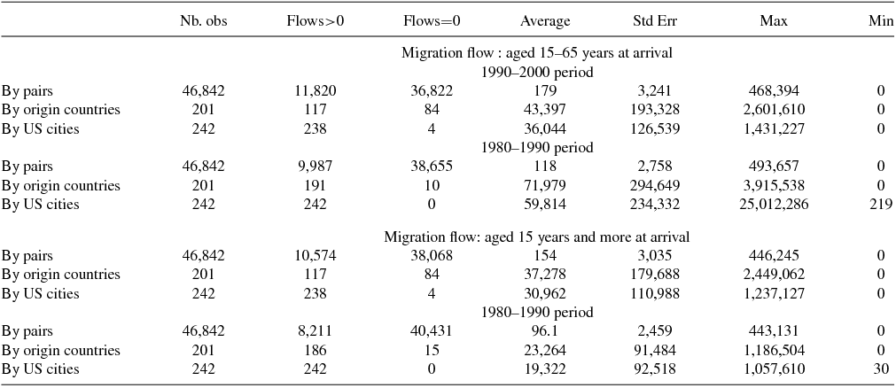
The data in this paper come from the 5 percent samples of the US Censuses of 1980, 1990, and 2000, which include detailed information on the social and economic status of foreign-born people in the US. Of this array of information, we utilize characteristics such as gender, education level, age, country of birth, and geographic location of residence in the US identified by metropolitan area. For the diaspora variable, we use all migrants in a given metropolitan area as reported in the 1990 census (or the 1980 census in the relevant sections). For the migration flow variable, we use the number of migrants aged 15 years and over at arrival (depending on the relevant definition) who arrived between 1990 and 2000 according to the 2000 census (or who arrived during 1980–1990 according to 1990 census). Clearly, using the immigrant population in 2000 that arrived between 1990 and 2000, we fail to capture temporary migrants who entered the US after 1990 and left before 2000. However, this is only a matter of definition of what the network effect is. As in related papers, we only record newcomers who settled in the US for a sufficiently long period of time and identify “long-term” network effects (the relevant concept at stake). Table 1 gives the number of bilateral corridors with positive and zero migration, and descriptive statistics on the size of bilateral migration flows.
Table 1. Descriptive data on migration flows

Notes: Table A1 provides the following information: total number of observations, observations with positive flows, observations with zero flows, average flow, standard deviation of flows, maximum flow, and minimum flow. The first row of each panel gives the information at the pair level. The second row gives the information by country of origin (summing up over cities of destination). The third row gives the info by US metropolitan area (summing up over countries of origin).
We re-group the educational variable provided by the US Census (up to 15 categories in the 2000 Census) to account for only three categories. These are (i) low-skilled migrants with less than 11 schooling years; (ii) medium-skilled migrants with more than 11 schooling years up to high school degree; (iii) the high-skilled migrants who have some college degree or more. An indicator of the location of education is not available in the US census so we infer this from the information on the age at which the immigrant reports to have entered the US. More specifically, we designate individuals as “US educated” if they arrived before they would have normally finished their declared education level. For example, if a university graduate arrived at the age of 23 years or older, then he/she is considered “home educated.” On the other hand, if the age of arrival is below 23, we assume the education was obtained in the US. We also construct data on geographic distances between origin countries and US metropolitan areas of destination. The spherical distances used in this paper were calculated using the STATA software based on geographical coordinates (latitudes and longitudes) found on the web: www.mapsofworld.com/utilities/world-latitude-longitude.htm for country capital cities, and www.realestate3d.com/gps/latlong.htm for US cities. Other bilateral characteristics (such as language) are captured by the origin-country fixed effects.
The identification strategy of this paper rests on the implicit assumption that migrants settle down in a city on a permanent basis taking the network externality into account. This might be undermined if a large proportion of migrants are registered first in some particular metropolitan area (basically an entry point) and move afterwards to another city within the 10 year period. One reason for this could be that families host their relatives from abroad first, and then send them to another state for the purpose of risk diversification at the family level. Unfortunately, the Census data do not yield a precise estimate of the internal mobility rate of recent migrants. Nevertheless, existing information for the 1990–2000 period suggests that the internal mobility issue is not too serious.
Over the 1990–2000 period, out of 12.78 millions new migrants, 5.26 millions arrived after 1995. It can be expected that a very large share of this group did not change their location in the US after their arrival. For the remaining 7.52 millions migrants who arrived between 1990 and 1995, the Census data provide their location in 1995. We see that 5.93 million have stayed in the same metropolitan area. Out of the remaining 1.59 million people, respectively 0.75 moved to another county in the same state and 0.84 moved to another state.
Unfortunately, this mobility data are not available at the metropolitan area level, but only at the county level. We should note many metropolitan areas include multiple counties so it is possible that many of those people changing counties actually remained in the same metropolitan area. The same holds for states since some of the largest metropolitan areas with high migrant density, like Chicago, New Jersey, New York, and Washington D.C. are spread over multiple states. All in all, figures cited above do not provide a direct measure of the new migrants’ mobility across metropolitan areas and we need to make assumptions. As mentioned above, we first assume that the migrants coming after 1995 did not move internally. Next, if all the 1.59 million new migrants who moved to another county (within the same state or in different states) also moved to another metropolitan area (worst-case scenario), we find that the internal mobility rate is around 11 percent. On the other hand, if we assume that people change metropolitan areas only when they move to another state, this rate falls to around 5 percent. Nevertheless, because some metropolitan areas include multiple counties or multiple states, both of these rates should be seen as upper bounds of internal mobility. In short, these figures suggest that our identification strategy is not undermined by large internal mobility rates of new migrants within the 10 year period under investigation. Finally, it is worth emphasizing that, if immigrants were to move, we might be overestimating the effect of the policy channel and underestimating the role of the assimilation channel. Since we find the assimilation channel to be the more important one, actual effect might be bigger than what our results suggest.
As far as the econometric methodology is concerned, equation (5), supplemented by an error term εsij, forms the basis of the estimation of the network effects. The structure of the error term can be decomposed in a simple fashion:
 $$\begin{equation}
\epsilon _{ij}^{s}=\nu _{ij}^{s}+u_{ij}^{s},
\end{equation}$$
$$\begin{equation}
\epsilon _{ij}^{s}=\nu _{ij}^{s}+u_{ij}^{s},
\end{equation}$$where usij are independently distributed random variables with zero mean and finite variance, and νsij reflects unobservable factors affecting the migration flows.
There are a couple of estimation issues raised by the nature of the data and the specification. Some of those issues lead to inconsistency of usual estimates such as the Ordinary-Least-Squares (hereafter OLS) estimates estimates. One issue is the potential correlation of νsij with Mij. Using external instruments to solve such endogeneity problems did not affect the results in Beine et al. (Reference Beine, Docquier and Ozden2011). Here, as a robustness check, we will imperfectly deal with endogeneity in Section 4.6, relying on an two-stage-least-square strategy with internal instruments.
Another important concern is related to the high-prevalence zero values for the dependent variable Nsij. Table 1 shows that, depending on the period (1980’s or 1990’s), between 50 and 70 percent of the total number of observations are equal to zero. Consistent with our model, distances, and other barriers make migration costs prohibitive, especially between small origin countries and small metropolitan destinations. The high proportion of zero observations appears in many other bilateral contexts, such as international trade or military conflict, and creates similar estimation problems. The use of the log specification drops the zero observations which constraints the estimation to a subsample involving only the country–city pairs with positive flows. This in turn leads to underestimation of the key parameters αs and βs. One usual solution to that problem is to take ln(1 + Nsij) as the dependent variable and to estimate (5) by OLS. This makes the use of the global sample possible. Nevertheless, this adjustment is subject to a second statistical issue, the correlation of the error term usij with the covariates of (5).
Santos-Silva and Tenreyro (Reference Santos Silva and Tenreyro2006) specifically tackled this problem and proposed an appropriate technique that minimizes the estimation bias of the parameters. They showed, in particular, that if the variance of usij depends on csj, msi, dij, or Mij, then its expected value will also depend on some of the regressors in the presence of zeroes. This in turn invalidates one important assumption of consistency of OLS estimates. Furthermore, the inconsistency of parameter estimates is also found using alternative techniques such as (threshold) Tobit or non-linear estimates. In contrast, in case of heteroskedasticity and a significant proportion of zero values, the Poisson pseudo maximum likelihood (hereafter PPML) estimator generates unbiased estimators of the parameters of (5).Footnote 11 Furthermore, the PPML estimates is found to perform quite well under various heteroskedasticy patterns and under rounding errors for the dependent variable. Therefore, in the subsequent estimates of (5), we use the PPML estimation techniques and report the estimates for αs, βs, and δs.Footnote 12
Finally, the specification (5) includes a fixed effect term μsi, which allows to account for the effect of a particular form of Multilateral Resistance. In particular, Bertoli and Fernández-Huertas Moraga (Reference Bertoli and Moraga2013) show that this strategy accounts for the occurrence of Multilateral Resistance of Migration (MRM) if the MRM term does not vary across destinations. This corresponds to a particular form of the generating function for the exponential of the deterministic part of usij. This approach was followed by Ortega and Peri (Reference Ortega and Peri2013) for instance. More complex forms of the generating function require other econometric approaches that are quite difficult to implement in our case.Footnote 13
4. RESULTS
We first estimate (5) using the PPML estimator with country-of-origin and destination-city fixed effects. We initially ignore skill and education differences by performing the estimation with aggregate migration flows in Section 4.1. Then, in Section 4.2 , we allow coefficients to vary by education level. This specification accounts for differences in income per capita at origin which might lead to heterogeneity in the educational quality and other characteristics of the migrant flows. The comparison between two decades of migration, the 1980s and the 1990s, is conducted in Section 4.3. Sections 4.4 and 4.5 examine the robustness of our results to the remoteness of origin countries and to the size of US destination cities. Regressions with internal instruments are discussed on Section 4.6. Finally, we analyze the robustness of our results to the identification assumption (i.e. homogeneity of the functional form of the assimilation and policy channels) in Section 4.7.
4.1. Benchmark Regressions
In our benchmark regressions, we do not differentiate between education levels and assume that the coefficients (μsi, μjs, δs, αs, βs) are identical across different education groups. The dependent variable Nij in (5) measures the total migration flow from origin country i to US metropolitan area j between 1990 and 2000. As explained above, the PPML estimator addresses the issues created by the presence of large number of zeroes in the migration flows. We use robust estimates, important with the PPML estimator, since failure to do so often leads to underestimated standard errors and unrealistic t-stat above 100. Regression results are presented in Table 2. The standard errors are not reported to save space since they usually lead to estimates of δs, αs, and βs with t-stat higher than 10.
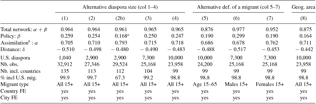
Table 2. Overall network effects – per sub-samples
Notes: PPML estimates of equation (5). All parameters significant at the 1 percent level except if (a): five percent level; robust estimates. (b) Computed as the difference between the total network and policy effects. Estimation carried out on migrants aged 15 years and over, on the 1990–2000 period; threshold in terms of the size of the total diaspora at destination (across all US metropolitan areas).
The use of the full sample involves the inclusion of small origin countries with idiosyncratic migration patterns. In particular, the coefficients δs, αs, and βs could be different from the ones for larger countries. Furthermore, many of these countries have fewer than a total of 500 migrants in the US, and their distribution across the US cities is not properly captured in the census data due to imperfect sampling.Footnote 14 We adjust the initial sample and leave out micro states which we define in terms of the total size of their migrant stock in the US in the year 1990. We use different threshold values: 1040, 2900, 7300, and 10000 migrants in the US. Depending on the threshold, the number of source countries included in the sample equals 135, 113, 104, or 99, respectively. These samples account for 99.9 to 98.9 percent of all immigrants and the respective regression results are reported in columns 1 to 4 of Table 2.
The estimate of the total diaspora effect (given by α + β) is reported on the first line of the table and is consistent with existing literature. The key parameters are quite stable across subsamples which is mainly due to the fact that we capture almost all of the migrants in the US, although we leave out a number of very small source countries. We find that 1 percent increase in the initial network size in 1990 approximately leads to a 1 percent increase in the bilateral migration flow between 1990 and 2000. The results further suggest that one fourth of the network effect, i.e. β/(α + β), is due to the national policy channel, and the rest, i.e. α/(α + β), is due to the assimilation channel. In other words, despite the fact that β can be taken as an upper bound, the magnitude of the policy channel is around 0.25 only. This is slightly lower than the 10-year sponsorship rates obtained by Jasso and Rozenzweig (Reference Jasso and Rosenzweig1986, Reference Jasso and Rosenzweig1989) because observed sponsorship rates capture the joint effect of networks on migration aspirations and realization rates. We identify only the “realization” part of it in this estimation. The elasticity with respect to distance is around − 0.5 regardless of the sample size.
Results in columns 1 to 4 were based on the flows of immigrants aged 15 years and over at time of arrival, regardless of their current age and gender. Next, we use alternative definitions of migration flows and show that, overall, the results are fairly robust to the choice of alternative measures. In column 5, the immigrant sample is restricted to ages 15 to 65 years at the time of arrival. Excluding elderly immigrants slightly reduces the magnitude of the policy channel as expected. In columns 6 and 7, we distinguish between male and female migrants above age 15 years at arrival. The main difference is that the national policy effect is found to be slightly greater for men than for women, while the assimilation effect is greater for women.
Our identification strategy relies on the definition of metropolitan areas used by the US census bureau, which defines the location of our local network/diaspora. In other words, we assume the migrant and his local network are located within the same US metropolitan area. In order to test the robustness to this particular assumption, we modify the definition of the geographic area corresponding to the local network.
In column 7, we now consider that the Mij variable is composed of the number of migrants from country i living in metropolitan area j as well as in neighboring metropolitan areas that are located within 100 miles from the center of j.Footnote 15 In about 50 percent of the cases, this modification leads to a sizeable increase in the network mass. Changing the definition of the geographic area in column 8, we find that both effects are roughly similar to the estimates of the regressions presented in columns 1 to 4. The assimilation effect is similar and the policy effect is slightly smaller than in the benchmark regressions.
4.2. Education Level
The existing literature has shown that the magnitude of the network effect on future migration flows tends to decline with the skill levels of immigrants (Carrington et al., Reference Carrington, Detragiache and Vishwanath1996; Winters et al., Reference Winters, de Janvry and Sadoulet2001; McKenzie and Rapoport, Reference McKenzie and Rapoport2010; Beine et al., Reference Beine, Docquier and Ozden2011). It is usually argued that low-skilled migrants face higher assimilation costs and policy restrictions at destination countries. Hence, they rely more on their social networks to overcome these barriers.
In line with the existing literature, we first differentiate between migrant flows based on their education levels to identify different skill categories. There is a certain level of imperfection in the census data since the education level is given by the number of years of completed schooling as reported by the migrants who come from different countries with different education systems. Comparison across origin countries is difficult. Nonetheless, we aggregate new immigrants into three different categories, as it is usually done in the literature (Docquier et al., Reference Docquier, Lowell and Marfouk2009). These categories are (i) low-skilled immigrants with less than 11 schooling years (labeled as “Primary”); (ii) medium-skilled immigrants with more than 11 schooling years up to high school degree (labeled as “Secondary”); (iii) the high-skilled immigrants who have at least one year of college education (labeled as “Tertiary”).
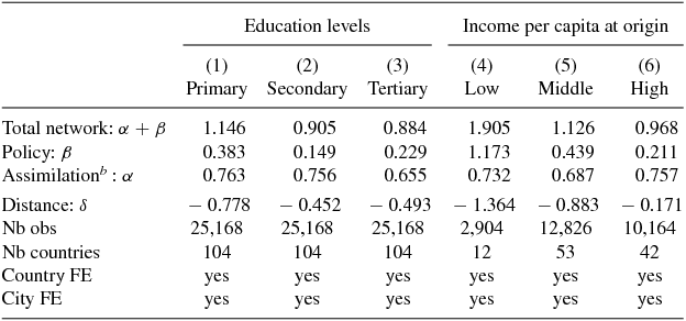
We separately estimate equation (5) for these three education levels. Results are presented in columns 1 to 3 of Table 3. Note that we only record immigrants who completed their education prior to migration and did not receive any further education in the United States. This distinction allows us to separate out migrants who entered as children with their families or who entered for education purposes under special student visas. In line with existing literature, we find that the total network effect (α + β) decreases with the education level of migrants, from 1.146 for the low skilled to 0.884 for the college educated. In addition, we find the local assimilation effect, given by α, is greater for low-skilled migrants (0.763) than for college graduates (0.655). The difference in the policy effect is, however, more pronounced (0.383 for the less educated, 0.149 for the medium skilled, and 0.229 for college graduates). These results indicate that the network effect is greater for the less-educated migrants, mostly because it helps them to overcome the national policy restrictions. Moreover, low-skilled migrants are much more sensitive to distance as seen from the sharp decline in the coefficient of distance as education level increases.
Table 3. Results – education level and quality
Notes: PPML estimates on countries with less than 7300 migrants All parameters significant at the 1 percent level, otherwise mentioned; robust estimates. (b) Computed as the difference between the total network and policy effects.
Our educational breakdown does not account for the heterogeneity in the quality of education across origin countries. Migrants from different countries might have similar degrees on paper but different skill levels and human capital. For example, a university degree obtained in a high-income OECD country might imply a higher level of human capital than a degree obtained in a low-income country.Footnote 16 Such disparities in educational quality matter as our sample only includes immigrants who have completed their education at home. If the quality of education differs significantly among immigrants with the same education levels, the ability to migrate outside family reunification programs or other legal channels might also be different. In the case of poorer countries with lower educational standards, one would expect the policy component of the total network effect to be stronger.
There is no official measure of quality of education by origin country. In a highly innovative paper relevant for us, Coulombe and Tremblay (Reference Coulombe and Tremblay2009) showed that the skill-schooling gap is highly correlated with the level of GDP per capita in the origin country. Based on their results, we estimate (5) distinguishing between three types of source countries. These groups are (i) low-income countries, (ii) middle-income countries, and (iii) high-income countries. We follow the World Bank income classification and, for each group of countries, we use the same thresholds in terms of size of the US diaspora. Obviously, income levels of the origin countries capture many other effects such as the level of development of financial markets, domestic political conditions, quality of economic institutions, etc.
Results of these additional regressions are reported in columns 4 to 6 of Table 3. We find that the overall network effect decreases with income level from 1.905 for low-income countries to 0.968 for high-income countries. In line with the previous estimates of columns 1 to 3, we find that most of the variation is driven by the national visa/policy effects. The policy effect equals 0.211 for high-income countries; it declines to 0.439 for middle-income and, finally, to 1.173 for low-income countries. These results imply that networks play an important role in providing legal access to the US to migrants from low-income countries. On the other hand, the assimilation effect shows almost no variation. We obtain an elasticity of 0.732 for low-income countries and 0.757 for high-income countries. Finally, we see that migrants from developing countries are more sensitive to distance as we would expect. On a final note, the diaspora is also composed of members with different education levels and they might differential impact on migration patterns. We have performed the estimation with multiple diaspora variables, differentiated according to education levels. The results were not different.
4.3. Flows in the 1990’s vs 1980’s
Our analysis in the previous sections focused on the effect of the diaspora size in 1990 on immigration flows to the US between 1990 and 2000. Our dataset includes similar variables for the migration stocks and flows in the 1980’s. Hence, we can conduct the same regressions on the flows observed in the 1980’s to investigate whether there has been any important changes in the migration patterns and the relative size of network effects. An alternative strategy would have been to combine observations from the 1980’s with those from the 1990’s and use a panel approach by pooling the data from the two cross-sections. Since we expect network effects to vary over time, we prefer the present approach.
Although we are not aware of a sizeable cultural shift that could affect the assimilation effect in the US, it is well documented that the US immigration policy changed significantly between the 1980s and the 1990s. The main changes are due to the 1990 US Immigration Act and the 1986 Immigration Reform and Control Act, which clearly expanded opportunities for family reunification. The main feature of the 1990 Act is that the number of immediate relatives of US citizens who can migrate is not limited or capped under the law. Therefore, quotas for family reunification can be exceeded in practice if the applications by immediate family members are above the estimated number by the law in a given year. As a result, as more immigrants previous cohorts obtain US citizenship, there is a natural upward trend in the number of people coming under the family reunification scheme sensu lato. The 1986 Act corresponds to the amnesty or legalization programs undertaken. As large numbers of undocumented migrants obtained legal resident status, they also became eligible to bring additional family members through the legal channels. Those who became citizens through the amnesty were even able to bring their relatives through the uncapped channel. Therefore, these policy developments suggest that the estimated β coefficient might have increased between the 1980’s and 1990’s.
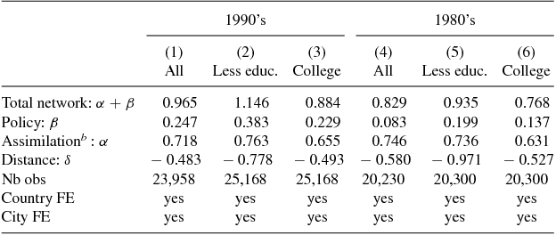
Table 4 reports the estimates obtained for the 1990’s and the 1980’s. For each period, we estimate the model on all migrants, on those with college education and on the less educated. Our estimates suggest that the national policy effects were greater during the 1990’s than during the 1980’s for all immigrant categories. The change is more important for less-educated migrants, for whom the policy effect doubled within a decade. This change is likely to capture the joint effects of the 1986 and 1990 Immigration Acts. On the other hand, the assimilation effect (α) remained stable across the two decades at around 0.75 for the low skilled and 0.65 for college graduates.
Table 4. Flows in the 1990’s vs 1980’s
Notes: All = All skill types; LS = low skilled; HS = high skilled. PPML estimates on countries with more than 7300 migrants. All parameters significant at the 1 percent level. (b) Computed as the difference between the total network and policy effects. Robust estimates. Estimation carried out on migration flows of individuals aged 15 years and over.
4.4. Distance Thresholds
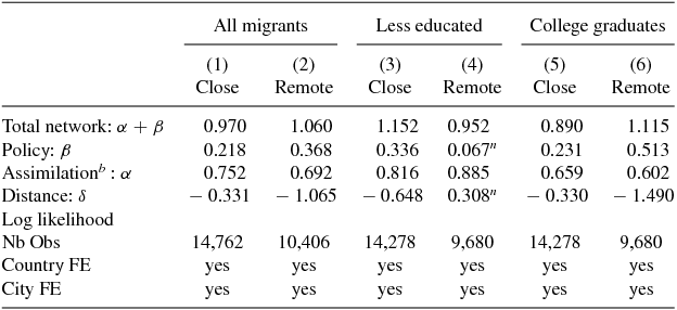
Geographic distance is one of the major barrier to migration. Furthermore, distance is a source of positive selection as its effect as a barrier is greater for the less educated. This differential impact of distance was illustrated in Table 3. Even though country fixed effects partly control for bilateral distances in our estimations, the sheer size of the US still leads to significant variations in terms of the distance and accessibility from origin countries to different American cities. For instance, the Caribbean countries that are close to the US are likely to send more migrants to cities in the south-east compared to the north-west. In the subsequent set of estimations, we define remote and close countries on the basis of the minimal distance to the US border with a cut-off of 6,790 kilometers. This is the median distance in terms of pairs of origin countries and US metropolitan areas. We also consider the effect of distance for two educational levels, college graduates, and the less educated. Results are presented in Table 5.
Table 5. Close versus remote countries
Notes: PPML estimates on the flow of migrants aged 15 years and over from countries with more than 10,000 migrants in the US. All parameters significant at the 1 percent level, except those superscripted n (non-significant). (b) Computed as the difference between the total network and policy effects. If not mentioned, robust estimates. Cut-off value to define far and close: 6,790 kilometers.
First, we find that distance plays a much more important role for migrants coming from remote countries (columns 1 and 2). The coefficient of distance is significantly smaller when the origin countries are closer to the US which are the Latin American and Caribbean countries. Second, the total network effect is slightly larger when origin countries are far away but this is not statistically significant. However, there is a difference in terms of composition. The national policy effect is greater for distant countries while the local assimilation effect is more important for closer countries.
We obtain more nuanced results when we compare the importance of distance for different education levels in columns 3 to 6. For low-skilled migrants, distance seems to be a very significant deterrent to the extent that it becomes prohibitive. We find that for the low-skilled migrants from distant countries, the policy effect becomes insignificant. On the other hand, for college-educated migrants from distant countries, the visa effect is much greater when compared to neighboring countries.
Finally, we see that the difference in the local assimilation effect between distant and nearby countries becomes small when we control for education. Hence, differences between columns 1 and 2 are mainly due to the skill composition of migration between close and remote origin countries. Once similar migrants pass the border and enter the US, the local assimilation effect does not vary with distance.
4.5. Dropping Small Cities
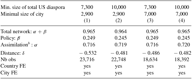
In order to assess the robustness of our results, it is also relevant to check whether our findings are driven by the inclusion of small cities, which we define as metropolitan areas with a small number of immigrants. Our source of concern is that small cities have larger numbers of zero observations at the dyadic level for both ln(1 + Mij) and ln(1 + Πij). This may lead to spurious correlation between these two variables. Therefore, we re-estimate equation (5) after dropping small countries as well as small cities. As described in the first two rows of Table 6, we drop countries with less than 7,300 or 10,000 migrants in the US, and we drop small cities with less than 2,900 migrants or less than 7,000 migrants. Combining the two cut-off values yields four alternative regressions with very robust results where the values of the assimilation and the policy channels are barely affected.
Table 6. Dropping small cities
Notes: PPML estimates. All parameters significant at the 1 percent level; otherwise mentioned; robust estimates. (b) Computed as the difference between the total network and policy effects. Estimation carried out on migrants aged 15 years and over, on the 1990–2000 period; threshold in terms of the size of the total diaspora at destination (across all US metropolitan areas).
4.6. Unobserved Heterogeneity
Another potential econometric issue is generated by the presence of unobserved bilateral factors νsij influencing the bilateral migration flows Nsij. In absence of observations for those factors, their effect will be included in the composite error term given by νsij + uij s = ηsij.Footnote 17 If those factors also influence the network size Mij, this leads to a correlation between the error term and one covariate, invalidating the use of OLS and PPML estimators. This is known as the correlated effect problem (Manski, Reference Manski1993).
A traditional approach to take care of the correlated effect bias is to use instrumental variables to predict value of Mij using a variable that is uncorrelated with Nij. Given that we estimate model (5) in a PPML set-up, the solution is not straightforward. Tenreyro (Reference Tenreyro2007) proposes a method to combine PPML estimators with instrumental variables estimator which can be implemented with the Generalized Method of Moments (hereafter GMM). Dropping the s subscript for convenience of exposition and aggregating all explanatory variables cj, Mi, dij, and Πij into the xij vector, the PPML estimator γ solves the following moment condition:
 $$\begin{equation}
\sum _{ij}^{n}[N_{ij}-exp(x_{ij}\gamma )]x_{ij}=0.
\end{equation}$$
$$\begin{equation}
\sum _{ij}^{n}[N_{ij}-exp(x_{ij}\gamma )]x_{ij}=0.
\end{equation}$$In order to instrument xij, one can use the following GMM estimator denoted by ψ as an alternative
 $$\begin{equation}
\sum _{ij}^{n}[N_{ij}-exp(x_{ij}\psi )]z_{ij}=0.
\end{equation}$$
$$\begin{equation}
\sum _{ij}^{n}[N_{ij}-exp(x_{ij}\psi )]z_{ij}=0.
\end{equation}$$In this expression, zij represent the vector of instruments, i.e. variables that are supposed to be correlated with Mij but uncorrelated with Nij. We rely on the GMM estimator ψ using two potential instruments which are the variables ln(1 + Mij) and ln(1 + Πij) observed in 1950, i.e. about 40 years before the observed diaspora patterns in the benchmark regression. Relying on an internal instrument is problematic if unobserved heterogeneity is driven by persistent dyadic factors such as cultural proximity or climatic variables. If it is the case, our instruments are likely to be correlated with νsij, invalidating the exclusion condition.
However, using migration stocks prior to the 1965 Hart–Celler Act as instruments might be an appropriate approach for the US. Indeed, the Hart–Celler Act (or 1965 Immigration and Nationality Act) abolished the system of national-origin quotas that had been in place in the US since 1921. As a result, the origin structure of immigration flows changed rapidly after 1965, with many more migrant arriving from developing regions (Asia, Africa, the Middle East, and Lain America) and much less from Western Europe. In addition, data reveal larger geographic dispersion in 1990 than in 1950 (Durand et al., Reference Durand, Massey and Charvet2000; Funkhouser, Reference Funkhouser2000, McConnell, Reference McConnell2008). For example, Mexican migrants in the 1950’s had obviously a strong preference for nearby metropolitan areas with similar climatic conditions. This is not the case anymore since Mexican migrants have spread out to every city in the US. Another example is that of Puerto Rico migrants who tend to concentrate in New York where the climate is quite different from the one prevailing in Puerto Rico.
Despite the 1965 policy reform, immigration stocks in 1950 are reasonably correlated with those of 1990 (a tiny part of the stock of 1990 was already present in 1950). In contrast, the network and policy effects on the flows during the 1990’s associated with the migrants already present in 1950 are supposed to be quite limited. Shortly, the IV results should be mainly seen as robustness checks since they are valid under the condition that unobserved factors of Nij should not be too persistent over time. Another drawback of using such an instrument is that it leads to a change in the sample. This is first due to the fact that the definitions of origin countries and US metropolitan areas have significantly changed between 1950 and 1990. A second reason is the independence of many former colonies during the 1950’s and 1960’s as distinct origin countries.Footnote 18
We first re-estimate the PPML regressions and use those estimates as a benchmark with respect to the IV-PPML (or GMM) estimates. Table 7 reports the estimates of the PPML on the restricted sample in column 1 (without instrumenting), and of the IV-PPML estimates à la Tenreyro in columns 2 and 3. In column 2, we use one instrument only, i.e. ln(1 + Mij) observed in 1950, while in column 3, we supplement the instrument set with ln(1 + Πij), again observed in 1950.Footnote 19 The results show that our estimates are strikingly robust to the instrumentation procedure. Both the total diaspora effect and the estimated policy effect are very similar across estimation methods. They are also very similar regardless of the inclusion of ln(1 + Πij) variable observed in 1950.
Table 7. Instrumenting network sizes
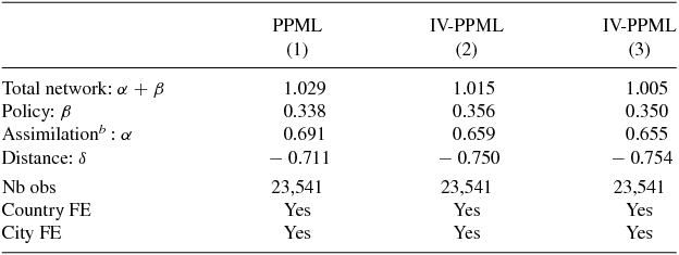
Notes: Column 1 : PPML estimates. Columns 2 and 3: IV-PPML or GMM estimates. All parameters significant at the 1 percent level. (b) Computed as the difference between the total network and policy effects. Robust estimates. Estimation carried out on migration flows of individuals aged 15 and over. Instrument for IV estimates in col 2: local network size observed in 1950. Instruments for IV estimates in col 3: local and national network sizes observed in 1950.
4.7. Homogeneity Assumption
Our identification strategy assumes that the functional forms for the local assimilation and the national policy effects of the diaspora networks are identical. In particular, we assume that both effects have log-linear form. It is important to assess whether this homogeneity assumption affects our results. One possibility is to estimate directly α and β in equation (4). Unfortunately, this is not possible if one accounts for unobserved heterogeneity across origin countries via inclusion of the fixed effects (μsi) in the estimated equation. As an alternative, we proceed via a two-step estimation of equation (4). In the first step, we estimate the following equation via PPML estimation:
 $$\begin{equation}
\ln N_{ij}^{s}=\widetilde{\mu }_{i}^{s}+\mu _{j}^{s}-\delta ^{s}\ln d_{ij}+\alpha ^{s}\ln \left( 1+M_{ij}\right),
\end{equation}$$
$$\begin{equation}
\ln N_{ij}^{s}=\widetilde{\mu }_{i}^{s}+\mu _{j}^{s}-\delta ^{s}\ln d_{ij}+\alpha ^{s}\ln \left( 1+M_{ij}\right),
\end{equation}$$ where the origin fixed effect ( $\widetilde{\mu }_{i}^{s}$) now accounts for the national policy component of the network
effect.
$\widetilde{\mu }_{i}^{s}$) now accounts for the national policy component of the network
effect.
This first estimation yields the coefficient for α for the
1990’s. Interestingly, using a cut-off value of 7,300 US migrants to
exclude small countries, we get an estimated value for the coefficient of
α equal to 0.719. This is strikingly close to the value of
α in Table 2. The
estimation of (9) also yields
an estimate for  $\widetilde{ \mu }_{i}^{s}$ which can be used in a second step as the dependent variable.
More precisely we can estimate the value of β with the following
country-level regression based on (4):
$\widetilde{ \mu }_{i}^{s}$ which can be used in a second step as the dependent variable.
More precisely we can estimate the value of β with the following
country-level regression based on (4):
 $$\begin{equation}
\widetilde{\mu }_{i}^{s}=\gamma +\beta ln(1+M_{i})+\rho ^{\prime }X_{ik}+\xi ln(N_{ii})+\omega _{i},
\end{equation}$$
$$\begin{equation}
\widetilde{\mu }_{i}^{s}=\gamma +\beta ln(1+M_{i})+\rho ^{\prime }X_{ik}+\xi ln(N_{ii})+\omega _{i},
\end{equation}$$ where ωi is an error term and where Xik are
country-specific time-invariant factors. The inclusion of the
Xik is supposed to account for the variability
in the  $\widetilde{\mu }_{i}^{s}$ that is unrelated to the policy effect. We consider four
potential factors: trade openness captured by the share of export to GDP, GDP
per capita in 1990, a dummy variable capturing whether the country speaks
English of not, and a regional dummy as defined by the World Bank official
classification. In line with Section 4.3., the sign of the GDP/capita variable
should be expected to be negative as rich countries are shown to have a lower
magnitude for the policy effect. The estimation tends to confirm this
expectation. Note also that we include a proxy for
Nii, i.e. the size of native population staying in
their origin country between 1990 and 2000.Footnote 20
$\widetilde{\mu }_{i}^{s}$ that is unrelated to the policy effect. We consider four
potential factors: trade openness captured by the share of export to GDP, GDP
per capita in 1990, a dummy variable capturing whether the country speaks
English of not, and a regional dummy as defined by the World Bank official
classification. In line with Section 4.3., the sign of the GDP/capita variable
should be expected to be negative as rich countries are shown to have a lower
magnitude for the policy effect. The estimation tends to confirm this
expectation. Note also that we include a proxy for
Nii, i.e. the size of native population staying in
their origin country between 1990 and 2000.Footnote 20
The following exercise should be nevertheless seen as a sub-optimal procedure, aimed only at guessing the importance of the linearity assumption for both externalities. The reason is threefold. First, the method is a two-step method, which is less efficient that the one step estimation methods like the one used earlier. Second, the inclusion of observable variables and the estimation of country fixed effects lead to small sample sizes. Finally, as reflected by the measure for Nii, our proxy that are specific to each origin country are likely to be plagued by measurement errors.
Table 8 reports the estimation results. The results suggest that the impact of economic development is, as expected, negative. The estimated value of β ranges between 0.19 and 0.26, which is clearly in line with the estimated β in Table 2. Although the two procedures are quite different, the results are relatively similar and this robustness check confirms that the local assimilation effect tends to dominate the global policy effect. Overall, this exercise suggests that our identification strategy yields sensible results, and that the functional homogeneity assumption does not seem to have a visible influence on the magnitude of the policy effect.
Table 8. A two-step identification strategy (dependent:  $\widetilde{\mu }_{i}^{s}$)
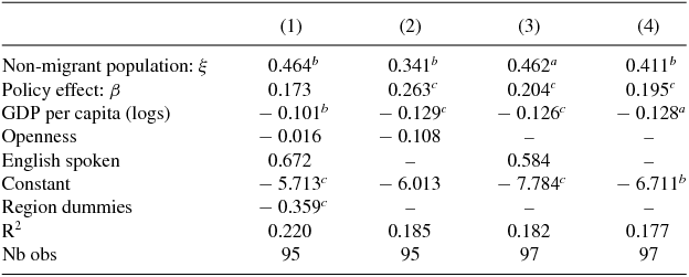
Notes: First-step estimation described by equation (9). Cut-off values of inclusion of origin countries: 7,300 migrants. Note that the first-step estimated α is 0.719. a, b, c: significant at 1 percent, 5 percent, and 10 percent level respectively.
5. CONCLUSION
This paper quantifies network externalities in international migration. In particular, it proposes a new microfounded approach aimed at disentangling the two main components of the overall network effect, i.e. the assimilation effect and the policy effect. Using migration data at the city level and at the country level, we are able to isolate the policy effect from the overall diaspora network effect for the US. We show that, during the 1990–2000 period, the average network elasticity is close to unity, with at most 25 percent attributed to the policy effect and at least 75 percent to the assimilation effect.
We find that the size and the composition of the network effect vary across a set of characteristics of the migrants. The policy effect is larger for low-skilled migrants and those coming from low income or distant countries. The implication for a destination country’s policymakers is that the migration multiplier (of the diaspora) cannot be completely reduced by via restrictive policies or complete elimination of family reunification preferences. The assimilation effect is strong and clearly dominates the policy effect in terms of the overall impact.
Our results do not mean that immigration policies are not effective. We have shown that policy changes have a non-negligible effect on the migration multiplier. Indeed, our regression results indicate that the policy elasticity has significantly increased between the 80’s and the 90’s. This can be due to the changes in the immigration laws or by other policies such as the legalization programs, which tended to increase the share of family-based migration flows to the US. Second, a large portion of migration policies are targeted towards specific origin countries which are captured via our fixed effects. The magnitude of the effect of such policies (that are independent of diaspora effects) are not captured by our estimation. That should be the goal of future research.