Introduction
In 1997, the World Health Organization (WHO, 2000a) declared that obesity was a global epidemic. The developing world, previously believed to be unaffected, also began to see an emerging epidemic of obesity as its spread reached global proportions (Prentice, Reference Prentice2006). Some view obesity in a more positive light, arguing that it is a subjective and cultural phenomenon rather than an objective medical condition (e.g. de Garine & Pollock, Reference De Garine and Pollock1995). However, ample evidence links obesity to diverse chronic diseases such as cardiovascular disease, type 2 diabetes mellitus, hypertension, stroke, dyslipidaemia, osteoarthritis and some types of cancer (Must et al., Reference Must, Spadano, Coakley, Field, Colditz and Dietz1999; Field et al., Reference Field, Coakley, Must, Spadano, Laird and Dietz2001). Obesity is also associated with an increased risk of death; for example, Peeters et al. (Reference Peeters, Barendregt, Willekens, Mackenbach, Al Mamun and Bonneux2003) estimated that 40-year-old female (male) non-smokers lost 7.1 (5.8) years due to obesity. Understanding the consequences, the World Health Organization (WHO, 2003) placed obesity at the top of the public health agenda as a major avoidable risk factor for many non-communicable diseases. Issues of medical costs and lost productivity caused by obesity naturally follow. Moreover, because the occurrence of obesity is related to various demographic factors such as age, sex, education and socioeconomic status, obesity inevitably affects socioeconomic areas such as income and health inequality, health insurance and taxation (Finkelstein et al., Reference Finkelstein, Ruhm and Kosa2005; Bhattacharya & Bundorf, Reference Bhattacharya and Bundorf2009). Some economists dismiss the problem of obesity as a rational choice, but numerous and costly attempts to lose weight suggest otherwise; evidence of myopia abounds (e.g. Laibson, Reference Laibson1997; Ruhm, Reference Rhum2012).
Given the extent and severity of obesity, it is urgent to have appropriate tools to assess it. And yet, medical and social science research diverge with regard to a measurement of obesity in general and body mass index (BMI) in particular. Body mass index is derived from a combination of weight and height in a variety of weightings for each measure (see Smalley et al., Reference Smalley, Knerr, Kendrick, Colliver and Owen1990, for some examples), but it is usually calculated as weight in kilograms divided by the square of height in metres (kg/m2); obesity is usually defined as BMI equal to or greater than 30. BMI has been falling out of favour in medical research, as its predictive ability for some chronic diseases is weaker than that of other anthropometrics. Kragelund & Omland (Reference Kragelund and Omland2005) even bade ‘farewell’ to BMI. On the other hand, although some economists have agreed that BMI is a poor measure of fatness (e.g. Burkhauser & Cawley, Reference Burkhauser and Cawley2008), it is still widely used in the social sciences for its simplicity and ready availability (e.g. Ruhm, Reference Rhum2012).
The reason for substituting away from BMI is that it does not distinguish between fat, lean tissue and bone. BMI measures total fat; however, visceral fat is more important for obesity-related diseases. Of course, it is technically feasible to measure visceral fat using laboratory methods such as dual-energy X-ray absorptiometry, computed axial tomography and functional magnetic resonance imaging. It is, however, economically infeasible to use such methods for a general, quick check-up. Cost is a particularly acute issue for the developing world. A portable bio-impedance monitor may require less time and money, but it is still an expensive tool for most people in the developing world. Because the limitations of BMI have been identified, medical researchers have tried to find more accurate and cost-effective alternatives to BMI, as explained in the next section. Unfortunately, no consensus has emerged thus far.
Given these issues, it is necessary to determine whether BMI is actually obsolete for the developing world. The argument that BMI is obsolete is largely based on research on populations in the developed world. Before hastily following the lead of this medical research, however, one needs to determine whether the argument applies to the developing world at all. If BMI turns out to be good enough for the developing world given its advantages vis-à-vis disadvantages, there is no need to undertake additional reform for the measurement of obesity.
Hence, this paper has two goals. The first is to use consistent definitions and measures to estimate the predictability of health and economic outcomes. Naturally following the first goal, the second goal is to identify the anthropometrics that predict health and economic outcomes most strongly. The strength of predictability is measured by the size of the association of obesity with the outcomes. At the outset, it is declared that no causality is intended for this goal; the sole focus of this paper is predictability. Although establishing causality for every outcome would be a great contribution to the literature, it is not necessary to achieve this goal. Randomization is out of the question because the dataset is a general survey. It is also difficult to find plausible instrumental variables for even one type of outcome, not to mention more than one type as in this paper. Although the survey is longitudinal, most health outcomes of interest are measured in the last follow-up, so it is not feasible for fixed effects models. Nevertheless, this paper is the first to consistently examine the associations of obesity with a range of health and economic outcomes together for a developing country.
Literature review
In the medical literature, BMI is regarded as a poor measure of fatness. The underlying fact is that visceral adipose tissue rather than total fat is known to generate obesity-related diseases. When BMI approximates total fat more accurately than it does visceral adipose tissue, muscular people can show a high BMI and be classified as obese, even if they have a normal amount of visceral adipose tissue (Burkhauser & Cawley, Reference Burkhauser and Cawley2008). In this case, anthropometrics that approximate visceral adipose tissue more accurately can be substituted for BMI for clinical and other purposes. Among many anthropometrics, waist-to-height ratio (WHtR), waist circumference (WC) and waist-to-hip ratio (WHpR) have been proposed; sagittal diameter and abdominal skinfold thickness have also been suggested (e.g. Ferland et al., Reference Ferland, Després, Tremblay, Pinault, Nadeau and Moorjani1989; Snijder et al., Reference Snijder, Visser, Dekker, Seidell, Fuerst and Tylavsky2002), but these are not included in the data used for this paper. Ashwell, Hsieh and their colleagues have published a series of papers that endorse using WHtR with a cut-off point of 0.5, regardless of sex, age, ethnicity or race (e.g. Ashwell et al., Reference Ashwell, LeJeune and Pherson1996; Hsieh et al., Reference Hsieh, Yoshinaga and Muto2003; Ashwell & Hsieh, Reference Ashwell and Hsieh2005). On the other hand, Lemieux et al. (Reference Lemieux, Prud'homme, Bouchard, Tremblay and Després1996) argued that WC was a more convenient anthropometric correlate of visceral adipose tissue than was WHpR because WC cut-off points for critical amounts of visceral adipose tissue were less affected by sex or the degree of obesity. After considering 27,000 participants from 52 countries in a case-control study, however, Yusuf et al. (Reference Yusuf2005) contended that WHpR was a better predictor than BMI of myocardial infarction attributable to obesity in most ethnic groups.
It is possible to list even more researchers on each side of the argument. For example, Ho et al. (Reference Ho, Lam and Janus2003) considered WHtR to be a better predictor of cardiovascular risk factors than BMI, WC and WHpR, but Dobbelsteyn et al. (Reference Dobbelsteyn, Joffres, MacLean and Flowerdew2001) supported the use of WC to predict cardiovascular risk factors. And yet, Dalton et al. (Reference Dalton, Cameron, Zimmet, Shaw, Jolley, Dunstan and Welborn2003) contended that unconditional on age, WHpR was more strongly correlated with cardiovascular disease risk factors than were BMI and WC. Instead of promoting one measure, Ho et al. (Reference Ho, Chen, Woo, Leung, Lam and Janus2001) were more liberal in the selection of measures. According to them, BMI and WC were useful predictors of cardiovascular risk factors for men, but WC and WHpR were for women. To make matters more complicated, Vazquez et al. (Reference Vazquez, Duval, Jacobs and Silventoinen2007) argued in their meta-analysis that BMI, WC and WHpR had similar associations with incident diabetes, implying that the three measures were equally good indicators of obesity.
Despite substantial research on the strength of associations between the simple anthropometrics and health outcomes, most studies have focused on one or at most a few health outcomes for people in the developed world, using various definitions and measures of obesity. This paper differs from the literature in two aspects. One is that it considers a range of outcomes with consistent definitions and measures. In doing so, it attempts to compare magnitudes of the risk of obesity for the outcomes and to assess the overall, rather than idiosyncratic, strength of the associations. The other is that light is shed on people in a developing country. There is no guarantee that the results obtained from populations in the developed world directly apply to those in the developing world. The two groups have different lifestyles, diets, health care systems and economic institutions, so they may have varying distributions of adipose tissue.
Methods
Survey data
The main data set for this paper is the Indonesian Family Life Survey. The survey started with 7224 households in 1993/1994, collecting detailed individual-level data from over 22,000 individuals. Since then, follow-ups were conducted in 1997 (IFLS2), 1998 (IFLS2+), 2000 (IFLS3) and 2007/2008 (IFLS4). Attrition is small enough so that 93.6% of IFLS1 households were re-contacted for IFLS4; the sample is representative of 83% of the Indonesian population. The IFLS is a longitudinal survey, but because IFLS4 contains detailed health outcomes, analysis for this paper is essentially cross-sectional. More important, two specially trained nurses visited each household, often multiple times, to obtain direct measurements of some health outcomes. Actual measurements probably reduced measurement errors, although it is difficult to estimate the size of the errors because the corresponding self-reported measures were not collected. However, it is possible to gain some insights into the size, using the only health indicator that was both measured and self-reported in IFLS4: hypertension. Measured hypertension is defined as systolic pressure ≥140 mmHg or diastolic pressure ≥90 mmHg, and both indicators are available for respondents aged 40 and over. According to measured hypertension, 42.6% of men and 49.2% of women in the sample have hypertension, while according to self-reported hypertension, only 13.3% of men and 23.1% of women do. The former reflects conditions at the time of the interview, whereas the latter pertains to the period before the interview. Thus, it is not entirely clear which reflects the true prevalence of hypertension in the sample. However, given the poor health care system in Indonesia, the former is preferred. Furthermore, Sohn (unpublished) has found that among respondents with measured hypertension, only 23.3% of men and 36.9% of women self-reported that they had hypertension. Although the accuracy of self-reported anthropometrics is likely to be higher than that of self-reported asymptomatic diseases such as hypertension, this considerable discrepancy between self-reported and measured hypertension implies that measurements of anthropometrics in the survey probably removed measurement errors to a non-negligible degree.
Measurements include basic anthropometrics such as height, weight and waist and hip circumferences, as well as blood pressure and cholesterol, among others. Waist and hip circumferences were measured for respondents aged 40 and over. In addition, only this age group answered questions regarding diagnosed chronic diseases. Therefore, the paper focuses on this age group. In order to avoid mistakenly attributing pregnancy to obesity, women aged 40–49 who were confirmed to be pregnant were excluded from the sample. Some basic health measures (e.g. height and weight) were available in IFLS1, but detailed measures began to be available only with IFLS2. Since then, the number of health measures has increased. The user's guides for IFLS2, IFLS3 and IFLS4 briefly explain the methods employed for some of the measures as follows:
(1) Height was measured with Shorr measuring boards.
(2) Weight was measured with Seca floor-model scales developed in collaboration with UNICEF. The floor-model scales had a digital read-out and were accurate to the nearest 0.1 kg.
(3) Blood pressure was measured with Omron digital measuring devices.
(4) Cholesterol was measured by pinprick blood samples and cholesterol meters.
Waist and hip circumferences were introduced with IFLS3, but neither of the user's guides for IFLS3 or ILFS4 explains the methods employed for these.
Measures of obesity
Obesity can be defined in many ways, and there is not much consensus on the definition. BMI cut-off points for obesity varied across the world until the WHO Expert Committee (1995) proposed a cut-off point of BMI≥30 for obesity for all people. Later, acknowledging differences in physical features by race, the World Health Organization (WHO, 2000b) differentiated BMI cut-off points for adult Europeans and adult Asians, thus defining obesity as BMI≥30 for adult Europeans and ≥25 for adult Asians. Note that 25 is the cut-off point for overweight for adult Europeans. Even for adult Asians, however, there is no agreed-upon cut-off point; the World Health Organization itself acknowledged this (WHO Expert Consultation, 2004). In this light, a strong argument has been made in the medical literature that BMI is not an effective measure of obesity. Although BMI's limitations have been acknowledged, it is unclear which measure should replace it for the measurement of obesity.
Among the proposed measures, this paper employs WHtR, WC and WHpR, because these are the main alternatives to BMI at present. Because consensus has not yet been reached regarding cut-off points for each measure to define obesity for adult Asians, as with BMI, this paper adopts the overweight cut-off point for adult Europeans as the obesity mark for Indonesians. Hence, obesity for Indonesians is defined for each measure as follows: BMI≥25, WHtR≥0.5, WC≥94 cm for men and WC≥80 for women; WHpR≥0.9 for men and WHpR≥0.8 for women (Dalton et al., Reference Dalton, Cameron, Zimmet, Shaw, Jolley, Dunstan and Welborn2003). In addition to BMI≥25 for adult Asians, the WHO Expert Consultation (2004) proposed an Indonesia-specific BMI cut-off point for obesity: BMI≥26 or BMI≥27. This paper adopts the latter because the former is close to BMI≥25 for adult Asians and it is based on a suspect assumption – that is, the percentage of body fat in Asians at the cut-off point for obesity is the same as the percentage of body fat in white people with a BMI of 30. On the other hand, the latter is data-driven in that the value is based on the analysis of co-variance with BMI as the dependent variable, ‘country’ as grouping variable, and age, sex and percentage of body fat as covariates. It is acknowledged that the cut-off points for the anthropometrics themselves are not agreed upon in the medical literature, but a starting point is necessary. Hence, this paper starts with the widely adopted cut-off points and applies different methods to check robustness.
Dependent and control variables
Interviewers asked about a total of thirteen acute symptoms during the 4 weeks prior to the interview, and respondents answered yes or no for each symptom. The thirteen acute symptoms were as follows: headache, runny nose, cough, difficulty breathing, fever, stomach ache, nausea/vomiting, diarrhoea (minimum 3 times per day), swollen legs, skin infection, eye infection, toothache and cold sores. Because the reference period was rather short, recall bias should not be severe. In addition, interviewers also asked about a total of twelve chronic diseases with which respondents might have been diagnosed. These were: hypertension, diabetes/high blood sugar, tuberculosis, asthma other lung conditions, heart-related problems (heart attack, coronary heart disease, angina or other heart problems), liver disease, stroke, cancer/malignant tumour, arthritis/rheumatism, uric acid/gout and depression. Because chronic diseases are conspicuous, diagnosed in person, and experienced every day, respondents should not have had difficulty in recalling them. Complementing the self-reported data on acute and chronic diseases, trained nurses measured total cholesterol (TC), high-density lipoprotein cholesterol (HDLC) and blood pressure, thus reducing measurement errors in them.
Because obesity is usually related to chronic diseases (confirmed below), each chronic disease should be further explored. On the basis of previous research, chronic diseases for which obesity is an established risk factor and for which the prevalence rate is higher than 1% in the sample were selected for analysis. These included hypertension, diabetes, heart-related problems, arthritis/rheumatism and uric acid/gout. Although the survey does not further distinguish between types of diabetes, given that respondents in the sample were at least 40 years old, almost all cases of diabetes were likely to be type 2 diabetes. In addition, heart-related problems refer to heart attack, coronary heart disease, angina or other heart problems.
In addition to health outcomes, this paper considers two labour market outcomes – employment status and earnings – to verify whether the good predictors of health outcomes are also good predictors of these economic outcomes. Employment is further divided into the broad and narrow sense of employment. The broad sense of employment refers to any activities related to work. Thus, a respondent is considered employed if he or she engaged in any of the following activities: worked/tried to work/helped to earn income primarily during the past week; worked/tried to worked/helped to earn income for at least one hour during the past week; had a job/business, but were temporarily not working during the past week; or worked at a family-owned business during the past week. The narrow sense of employment refers to income-generating activities. Thus, respondents are considered employed if their earnings were greater than zero. It is useful to consider the two senses of employment because informal employment is prevalent in Indonesia.
Earnings refer to salaries or wages during the past month (including the value of all benefits) for paid employees and net profits during the past month (after all business expenses) for the self-employed. As in Borjas & Bronars (Reference Borjas and Bronars1989) and Sohn (Reference Sohn2013a), a small number of negative profits are converted to one to make the value of its natural log 0. Analysis is also made for women, despite the sample selection bias in earnings. One reason is that predictability is the major issue in this paper, while causality is not. Another reason is that the literature is particularly interested in women because of possible discrimination against obese (white) women, but not necessarily against obese men (Finkelstein et al., Reference Finkelstein, Ruhm and Kosa2005). Hence, the consideration of Indonesian women would facilitate comparisons of this paper with the literature.
All analyses control for the following basic demographic characteristics: age, age squared, schooling, marital status, ethnicity, religion and urbanity. Current smoking status is additionally controlled for because, although debatable, smokers have higher metabolic rates and consume fewer calories than non-smokers, possibly having lower weight as a result (Chou et al., Reference Chou, Grossman and Saffer2004; Gruber & Frakes, Reference Gruber and Frakes2006; Baum, Reference Baum2009; Courtenmanche, Reference Courtemanche2009). Types of smoking in the survey include chewing tobacco, pipes, self-rolled cigarettes and commercial cigarettes/cigars; however, the absolute majority of the sample smoked commercial cigarettes/cigars (see Sohn, Reference Sohnforthcoming, for details). A dummy variable for vigorous activities during the 7 days prior to the interview is also held constant to proxy lifestyle for energy consumption.
Although sample sizes change depending on the dependent variables estimated, for most analyses, sample sizes are 4846 for men and 5345 for women. Observations are restricted to remove possible coding errors as follows: earnings ≤Rp 20,000,000; a small number of respondents are removed whose highest education level is adult education or school for the disabled; 120 cm≤height≤200 cm; 30 kg≤weight≤150 kg; 10≤BMI≤40; 50 cm≤WC≤130 cm; 60 cm≤hip circumference≤140 cm; and 10≤TC, HDLC≤500.
Analysis
In the following analyses, OLS is used when the dependent variable is continuous; the affected variables consist of TC/HDLC and the natural log of earnings. However, when (left) censoring is a serious issue, tobit models are applied instead of OLS; the affected variables consist of the number of acute symptoms and the number of chronic diseases. On the other hand, when the dependent variable is dichotomous, probit models are used. However, using linear probability or logit models does not affect the results (not shown); the affected variables consist of (measured) hypertension, all the selected chronic diseases and employment status.
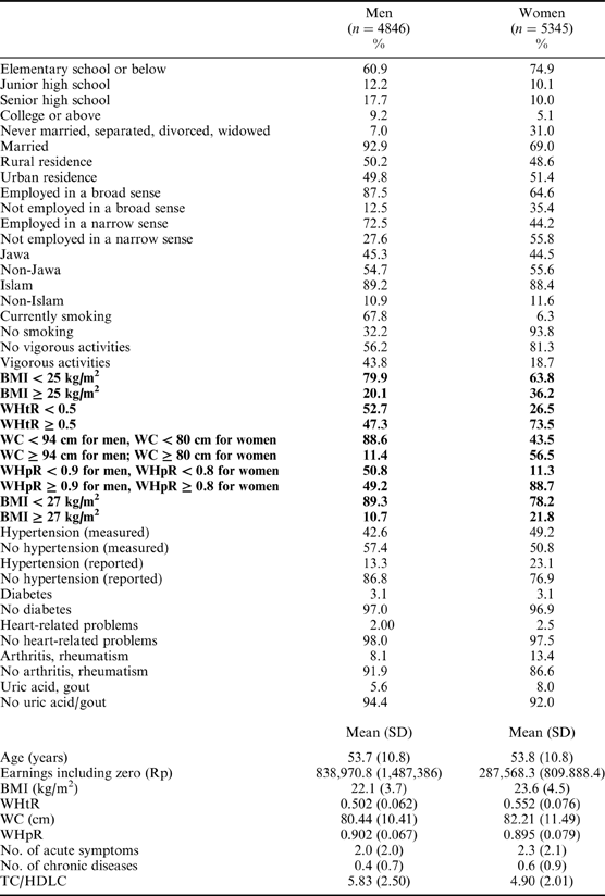
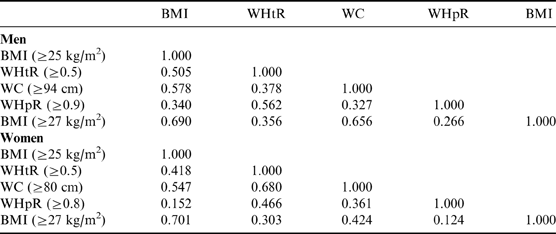
Men and women are analysed separately due to differing physical features (e.g. given the same height, women have greater amounts of total body fat than men) In addition, sampling weights (PWT07XA in dataset) are applied for all estimations, and standard errors are clustered at the county (kecamatan) level. Descriptive statistics are provided in Table 1, along with correlation coefficients among the obesity measures by sex in Table 2.
Table 1. Descriptive statistics of selected variables, Indonesian Family Life Survey

Table 2. Correlation coefficients among measures of obesity: the conventional cut-off points

Results
Descriptive statistics of obesity measures
Before comparing obesity measures for predictability, it is essential to understand how different obesity measures classify obesity. The bold section in Table 1 contains relevant figures with the conventional cut-off points. When a BMI of 25 is applied as a cut-off point, 20.1% of men are classified as obese, whereas 36.2% of women are obese. These figures are reasonable compared with those from other sources. For example, according to the World Health Organization (WHO, 2011, p. 146), the corresponding figures for the year 2008 are 16.1% and 25.3% for men and women aged 20 and older, respectively. The higher prevalence in the sample reflects the fact that obesity generally increases with age. With WHtR, both figures increase more than two times to 47.3% and 73.5%, but with WC the figures drop to 11.4% and 56.5%. When WHpR is used, both figures increase again to 49.2% and 88.7%. When a BMI of 27 is applied, the corresponding figures again diminish considerably to 10.7% and 21.8%. The figures derived from WHtR and WHpR do not seem to appropriately reflect the prevalence of obesity given the low income level of the Indonesian population; low income is usually associated with low prevalence of obesity in the developing world (more discussion in the concluding section). This fact anticipates their low predictability. The comparisons illustrate the instability of obesity classifications depending on the applied measures. Moreover, each measure is not closely related, as can be seen in Table 2. Naturally, BMIs of 25 and 27 are most highly correlated for both sexes, but their correlation coefficient is only about 0.70. Simply by reading the statistics, one can anticipate that each measure would yield varying degrees of predictability. This turns out to be true, as explained below.
Health outcomes
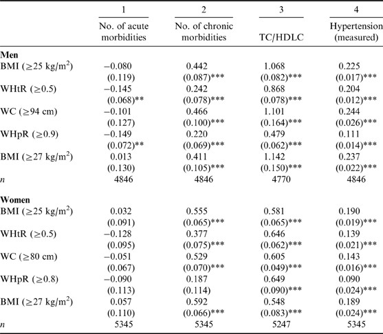
Table 3 presents the marginal effects of obesity on reported and measured health outcomes by sex, where obesity is defined by the conventional cut-off points for BMI, WHtR, WC and WHpR. Obesity is usually associated with chronic diseases; thus, it is expected that obesity will be closely related to the number of chronic diseases, but not necessarily the number of acute symptoms. Columns 1 and 2 of Table 3 confirm this conjecture and suggest that the obesity measures exhibit appropriate construct validity. According to Column 1, if obesity is related to the number of acute symptoms at all, the relationship seems negative. Hence, obese men, defined by either WHtR or WHpR, suffer 0.15 fewer acute symptoms. Because the mean number of acute symptoms is 2.0, this is not a small relationship. The overall pattern of the relationship in Column 1, however, indicates that obesity is not closely associated with acute symptoms. On the other hand, Column 2 consistently demonstrates that obesity is positively associated with chronic diseases. For men, obesity as defined by WC shows the strongest relationship with the number of chronic diseases; for women, BMI (≥27) is the best predictor. The corresponding figures suggest that obese men and women suffer 0.47 and 0.59 more chronic diseases, respectively, than their non-obese counterparts (about 100% relative to each mean).
Table 3. Marginal effects of obesity on reported and measured health: the conventional cut-off points

Notes: for Columns 1 and 2, a tobit model is used; for Column 3, OLS is used; for Column 4, a probit model is used.
The following variables are controlled for, but not listed: age, age squared, education, marital status, ethnicity, religion, urbanity, current smoking status, vigorous activities during the 7 days prior to the interview. Sampling weights are applied. Standard errors clustered at the county level are in parentheses.
**p<0.5; ***p<0.01.
Among chronic diseases, obesity is particularly associated with high levels of low-density lipoprotein cholesterol (LDLC), low levels of HDLC and high probability of hypertension. Columns 3 and 4 demonstrate these associations. Regarding the ratio of TC to HDLC, BMI (≥27) is also the best predictor for men, and WHtR for women. Therefore, according to these figures, obese men's ratio is 1.1 (20.0% relative to the mean) higher than that of non-obese men, and obese women's ratio is 0.65 (13.2% relative to the mean) higher than that of non-obese women. For hypertension, WC is the best predictor for men, while BMI (≥25) is the best predictor for women. According to these figures, obese men and women are 24.4%p (percentage points; 57.3% relative to the mean) and 19.0%p (38.6% relative to the mean), respectively, more likely to suffer hypertension than are their non-obese counterparts. When Columns 2–4 are considered, BMI and WC have the strongest relationships with health outcomes.
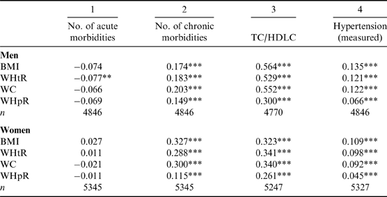
Another way of checking the strength of relationships with health outcomes is to include a continuous variable of anthropometrics (rather than a dummy variable for obesity) in the relevant statistical models and estimate the effect of a 1 standard deviation (SD) increase in each variable of interest (i.e. BMI, WHtR, WC and WHpR). While a dummy variable simplifies the classification of obesity, it loses important information and places too much emphasis on the cut-off points, thereby missing important actions that take place above and below the cut-off points. For example, when obese individuals gain more weight, their obesity status remains the same, but their health further deteriorates.
Table 4 lists results with the continuous measures of the four anthropometrics, and the overall result is the same as that for Table 3: BMI and possibly WC are the best predictors. Specifically, according to the strongest predictors, a 1 SD increase in WC is associated with 0.20 and 0.33 more chronic diseases for men and women, respectively (about 50% relative to each mean). In addition, a 1 SD increase in BMI raises TC/HDLC by 0.56 (9.7% relative to the mean) for men and 0.34 (7.0% relative to the mean) for women, respectively. The corresponding figures for hypertension are 13.5%p (31.7% relative to the mean) and 10.9%p (22.2% relative to the mean). When Tables 3 to 4 are considered together, BMI stands out for its strong relationships with health outcomes, while WHtR and WHpR have equally weak relationships with health outcomes. The patterns present in Tables 3 and 4 reappear when attention is paid to the presence of specific chronic diseases, rather than the number of chronic diseases.
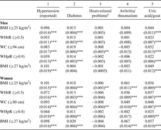
Table 5 considers the selected chronic diseases. As medical research has consistently demonstrated, obesity is more or less related to all of the listed diseases. In addition, only BMI and WC show the strongest relationships with the outcomes. Specifically, BMI shows the strongest relationship with 1 outcome for men and 4 for women; WC does so with 3 outcomes for men and 1 for women. When the strongest relationships are considered, obesity is related to a 10.1%p (75.9% relative to the mean) higher probability of hypertension for men; the corresponding figure for women is the same, i.e. 10.1%p (43.7% relative to the mean). With regard to hypertension, it is of interest to compare the sizes of the relationships in Table 5 with those in Table 3. For every anthropometric, the size of predictability in Table 5 is smaller than that in Table 3, and the largest in Table 5 is only 41.4% of that in Table 3. Hypertension in Table 5 refers to self-reported hypertension, whereas hypertension in Table 3 refers to measured hypertension. The smaller sizes in Table 5 suggest that many respondents were unaware that they had hypertension or they had the knowledge but the condition was undiagnosed, which would result in attribution bias. Given the poor health care system in Indonesia, both reasons are plausible. The comparisons suggest that the marginal effects of obesity on the other health outcomes in Table 5 are likely to be biased downwards. And yet, unless bias in diagnosis is systematically correlated with the measures used for obesity, the downward bias should not impede the identification of the strongest predictors. However, it is important to be aware of the downward bias when interpreting the marginal effects in Table 5.
Table 5. Marginal effects of obesity on reportedly diagnosed health: the conventional cut-off points

Notes: for all columns, a probit model is used. The sample sizes for men and women are 4846 and 5345 respectively.
The following variables are controlled for, but not listed: age, age squared, education, marital status, ethnicity, religion, urbanity, current smoking status, vigorous activities during the 7 days prior to the interview.
a Heart attack, coronary heart disease, angina or other heart problems. Sampling weights are applied. Standard errors clustered at the county level are in parentheses.
**p<0.5; ***p<0.01.
As for diabetes, the largest marginal effects of obesity are 1.9%p (61.3% relative to the mean) for men and 2.0%p (64.5% relative to the mean) for women. Regarding heart-related problems, only WC has a statistically significant effect: 0.8%p (40.0% relative to the mean) for men but −0.8%p (−32.0% relative to the mean) for women. This finding for women is inconsistent with conventional knowledge. However, it should not be dismissed as a statistical idiosyncrasy because all marginal effects for women, regardless of their statistical significance, are negative and subsequent analyses replicate the negative relationship (see Table 6). Low levels of meat consumption per capita in Indonesia may be a possible reason. On the other hand, while obesity is not associated with arthritis/rheumatism for men, the association for women is up to 6.7%p (50.0% relative to the mean). Obesity is also positively related to the probability of having uric acid/gout, as much as 5.2%p (92.9% relative to the mean) for men and 5.7%p (71.3% relative to the mean) for women. Overall, BMI and WC are unambiguously the strongest predictors of the chronic diseases.
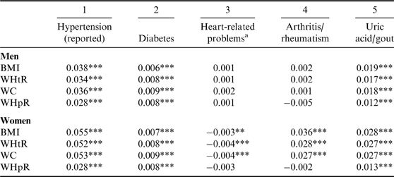
Table 6. Marginal effects of obesity on reportedly diagnosed health: 1 SD measure

Notes: same as for Table 5.
As shown in Table 6, 1 SD measures further support this argument. Small differences notwithstanding, BMI and WC are the best predictors of the chronic diseases for men and women. BMI has the strongest relationship with 2 outcomes for men and 3 for women; WC has the strongest relationship with 1 outcome for men and 2 for women (sizes are tied for one outcome). WHtR ratio scores only 1 tied outcome.
It is also worth noting the sizes of relationships between obesity and the chronic diseases, because they are economically meaningful. When the largest sizes are considered, a 1 SD increase in BMI increases the probability of having hypertension by 3.8%p (28.6% relative to the mean) for men and 5.5%p (23.8% relative to the mean) for women. The marginal effect of a 1 SD increase in WC on the probability of having diabetes is 0.9%p (29.0% relative to the mean) for both men and women. On the other hand, the marginal effect of a 1 SD increase in BMI on the probability of having heart-related problems is none for men but −0.4%p (−16.0% relative to the mean) for women. No relationship is shown for men between the anthropometrics and the probability of having arthritis/rheumatism, but the figure for women is 3.6%p (26.9% relative to the mean). In addition, a 1 SD increase in BMI is associated with a 1.9%p (33.9% relative to the mean) higher probability of having uric acid/gout for men; the corresponding figure for women is 2.8%p (35.0% relative to the mean).
Economic outcomes
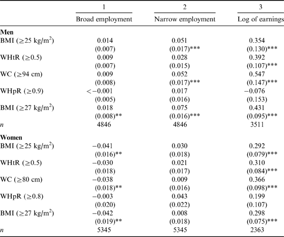
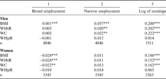
Thus far, it has been demonstrated that BMI and WC are the best predictors of health outcomes. A following question would be whether these results can be seen with other types of outcomes. Two important labour outcomes – employment and earnings – are considered in Table 7. Column 1 indicates that obesity is little related to the broad sense of employment for men, whereas obese women tend to be employed less than non-obese women. Specifically, according to the finding estimated by BMI (≥27), obese women work 4.2%p (6.5% relative to the mean) less than non-obese women. When the narrow sense of employment is considered, the results change to some extent. Again, obese men defined as BMI (≥27) are 7.5%p (10.3% relative to the mean) more likely to work, whereas obesity is not associated with employment for women. As the definition of employment is more connected with pay, i.e. moving from Column 1 to Column 2, the coefficients on the obesity measures grow. The results suggest that obese men and women were particularly good at picking jobs that actually generated earnings; alternatively, earnings could make the workers obese. In this light, it is not surprising that obesity is positively related to earnings, as listed in Column 3, and that WC shows the strongest relationship for both men and women. The size of the relationship is substantial. Obese men earn 72.8% (=e 0.547−1) more than non-obese men. Similarly, WC is also the best predictor of earnings for women: obese women earn 44.2% (=e 0.366−1) more than non-obese women. Note that only BMI and WC have the strongest relationships with the economic outcomes. This overall pattern repeats itself in Table 8 for 1 SD measures: BMI is the best predictor of 2 outcomes for men and women, while WC is the best predictor of 1 outcome for men, but none for women. Weight-to-height ratio is the best predictor of 1 outcome for women, but it is tied with BMI. In addition, the size of the positive relationship (without implying causality) between the obesity measures and earnings is large: a 1 SD increase in WC is associated with 22.2% higher earnings for men, while a 1 SD increase in BMI is associated with 18.6% higher earnings for women.
Table 7. Marginal effects of obesity on economic outcomes: the conventional cut-off points

Notes: For Columns 1 and 2, probit models are used; for Column 3, OLS is used. The following variables are controlled for, but not listed: age, age squared, education, marital status, ethnicity, religion, urbanity, current smoking status, vigorous activities during the 7 days prior to the interview. Sampling weights are applied. Standard errors clustered at the county level are in parentheses.
**p<0.5; ***p<0.01.
Discussion and Conclusions
Obesity has become a pandemic, increasingly affecting not only the developed world but also the developing world. As incomes rapidly increase, the prevalence of obesity in the developing world is likely to soar. Under these circumstances, it is necessary to have appropriate assessment tools for measuring obesity. Body mass index has been widely used for such purposes, but the medical literature has grown sceptical of the use of BMI for this purpose because it is a weak predictor of obesity-related diseases. In contrast, BMI is still commonly used in the social sciences for measuring obesity, possibly because of its simplicity and ready availability in surveys. Medical research has proposed several alternatives, but none dominates. Moreover, most research is based on populations in the developed world. In this situation, one should not hasten to discard BMI and adopt the alternatives for the developing world. Given the differences in lifestyles, diets, food availability and attitudes towards fatness and body features, BMI may be still useful in the developing world; the alternatives may not be better choices.
This paper selects three alternatives that have often been proposed in medical research: WHtR, WC and WHpR. Furthermore, two BMI cut-off points are compared: 25 and 27. Using consistent definitions and measurements, this paper estimates the associations of these alternatives with selected health and economic outcomes by sex for Indonesia. Consistent with the literature, in general, obesity in Indonesia is statistically significantly associated with these health and economic outcomes, and the sizes of the associations are large. More important, BMI and WC turn out to have the strongest relationships with most of the outcomes, whereas WHpR is the weakest. Table 9 presents the total number of times that each anthropometric has the strongest association with the dependent variables across Tables 3–8, including ties; p-values need to be less than 0.05 to be counted in. When BMI has the strongest relationship with an outcome for 1 SD measures, 1 count is added to the total counts of both BMI (≥25) and BMI (≥27). For both sexes, BMI (≥27) exhibits the strongest association with outcomes 22 times, considerably higher than the second-highest count of 15 for BMI (≥25). The figure for WHtR is only 4, mostly resulting from women. WHpR counts just twice in total: one for the number of acute symptoms for men, which is not usually associated with obesity, and the other for TC/HDLC for women. Examined by sex, BMI is more predictive for women, whether the cut-off point is 25 or 27. When BMI (≥27) is compared with WC, although the latter is far behind the former for women (12 vs 4), the latter is very close to the former for men (10 vs 9). This last finding implies that it may be more effective to apply different anthropometrics to different sexes for predicting health and economic outcomes. Although not reported, when happiness – usually considered the ultimate goal in life – is placed as a dependent variable, the results are the same (see Sohn, Reference Sohn2013b, for a general discussion of happiness in Indonesia). Also, following Burkhauser and Cawley (Reference Burkhauser and Cawley2008), cut-off points of WC, WHtR and WHpR for obesity are redefined as those that result in approximately the same rates of obesity as does the BMI (≥25) cut-off point for obesity, but the results (not shown) change little.
Table 9. Total numbers of strongest associations with dependent variables across Tables 3 to 8

Notes: associated p-values need to be less than 0.05 to be counted in.
The results thus challenge the criticism of BMI as an obesity measure. Furthermore, this paper reconciles the inconsistent findings in the literature. Most studies use at most a few dependent variables for assessing the predictive power of several obesity measures. As Table 9 illustrates, a certain obesity measure may have the highest predictive power for a certain dependent variable, but not for other dependent variables. As an extreme example, if only TC/HDLC for women is considered, one would mistakenly conclude that WHpR is the best obesity measure. The novel feature of this paper is the consideration of a variety of outcomes. When seen in this setting, BMI is still an appropriate measure of obesity, at least in Indonesia and possibly the developing world. Using BMI for the developing world may in fact be a good choice, given the options available to social science researchers. Further, this paper suggests that WC may be a better measurement of obesity than BMI for the following reasons. First, WC predicts various outcomes as much as BMI for men, but it requires only a measuring tape, which is much easier to carry than both a scale for weight and a stadiometer for height. Second, it is easier to measure WC than weight and height. Third, measurement errors in WC are smaller because only one number is needed, rather than two (weight and height) for BMI. These advantages are particularly appealing for the developing world for its simplicity (requiring less human capital) and low cost.
In addition, this paper finds a positive association between obesity and earnings. This is not a new finding; the new finding is that this association is consistent regardless of obesity measures. The positive association between obesity and earnings is inconsistent with findings from the developed world, where the relationship is ambiguous for men but negative for women. Finkelstein et al. (Reference Finkelstein, Ruhm and Kosa2005) reviewed eight studies that used a US data set (National Longitudinal Survey of Youth 1979: NLSY) and found that white obese women generally earn less than their non-obese counterparts but the association is weak for men. Cawley (Reference Cawley2004) applied three methods in the literature to the NLSY and reached the same conclusion. For the UK, Sargent & Blachflower (Reference Sargent and Blanchflower1994) and Morris (Reference Morris2006) drew on two different data sets but their conclusions were the same as those for the US. All the studies tried to tease out causality from obesity to earnings, but they did not establish definitive causality. There have been other attempts to find causality in the opposite direction, i.e. from earnings to obesity. Cawley et al. (Reference Cawley, Moran and Simon2010) found no causality for elderly Americans, but Schmeiser (Reference Schmeiser2009) estimated such causality for low-income women in the US. Hence, the large coefficients on obesity in Tables 7 and 8 may reflect positive interactions in both directions. In addition, the findings are consistent with those from the developing world. Sobal & Stunkard (Reference Sobal and Stunkard1989) reviewed such findings more than two decades ago. They conjectured that owing to relatively abundant food with few normative constraints about body weight, high socioeconomic status men and women in the developing world and low socioeconomic status women in the developed world tend to be overweight or obese. Alternatively, when one's weight relative to the population mean is a status symbol, as proposed by Blanchflower et al. (Reference Blanchflower, Oswald and van Landeghem2009), high earners in a country with a low mean weight may ‘buy’ weight, whereas those in a country with a high mean weight may buy diets.
Before concluding, this paper acknowledges some limitations, mostly arising from the data; the limitations naturally indicate the direction of future research. First, the IFLS is a general social science survey rather than a medical survey, so protocols for waist and hip circumference are not explained in detail in the user's guide. Because the nurses were specially trained for the purpose and the measurement is straightforward, however, measurement errors would not be large enough to affect the substance of the results. Second, the results in this paper rely on data of a single country. As the positive relationship between obesity and earnings varies, different countries are likely to produce varying results. Replications for other countries are desired; when they are performed, this paper recommends considering not a single outcome but a collection of outcomes at the same time. Third, a more serious concern is the self-reporting of diseases. This is generally unavoidable in social science surveys due to cost constraints. However, as demonstrated by the discrepancy between the prevalence of self-reported hypertension and that of measured hypertension, self-reporting is not ideal for medical research. Although the results in general show the expected signs and magnitudes, implying that errors may not be severe, future research can improve on this paper by employing measured outcomes. Fourth, this paper does not consider causality between obesity and the various outcomes mainly because the aim is to estimate the sizes of the correlations and partly because some important variables are available for only one time point. However, because the IFLS is an on-going longitudinal survey, the variables considered in this paper should be also available in the future. In that case, future research can estimate causality.
Acknowledgments
The author is grateful to two anonymous reviewers for helpful comments and suggestions.


