Introduction
There is now fairly substantial evidence of a socioeconomic gradient in low birth weight (LBW) for developed countries (see Kramer et al., Reference Kramer, Seguin, Lydon and Goulet2000; and for evidence for Ireland see McAvoy et al., Reference McAvoy, Sturley, Burke and Balanda2006, and Niedhammer et al., Reference Niedhammer, Murrin, O'Mahony, Daly, Morrison and Kelleher2012). The incidence of LBW (weighing less than 2500 g) tends to fall as socioeconomic status increases and the phenomenon is observed for a variety of measures of socioeconomic status (such as income, education and employment status).
Low birth weight is of concern for a number of reasons. There are a number of studies that link early life conditions with later outcomes in the areas of health and also education and labour market outcomes. For example, Barker (Reference Barker1997) highlighted the link between LBW and a number of conditions later in life. Delaney et al. (Reference Delaney, McGovern and Smith2011) showed with Irish data how public health improvements that affected infant mortality in the 1940s later had beneficial impacts on adult health outcomes. Almond and Currie (Reference Almond and Currie2011a, Reference Almond and Currieb), Black et al. (Reference Black, Devereux and Salvanes2007) and Currie (Reference Currie2009, Reference Currie2011) provided evidence from other countries and time periods showing correlations and sometimes plausible directions of causation between LBW and a range of health, education and labour market outcomes.
Given the evidence above that early life conditions may have persistent effects over the life course, it also seems likely that some of the socioeconomic gradient in health that is evident in adults had its origins in early life and may be manifested in a socioeconomic gradient in LBW. Thus for policymakers who wish to reduce socioeconomic health gradients for adults, one possible option might be to address this gradient at earlier ages. Elimination of even part of the socioeconomic gradient in health via those with lower socioeconomic status attaining similar health to those with higher status would lead to significant improvements in longevity, quality of life and labour market productivity. Thus evidence on the socioeconomic gradient of LBW should be helpful in this regard.
One of the principal measures for summarizing the link between socioeconomic status and a given health outcome is the concentration index. Curiously, despite the relatively abundant literature detailing the link between LBW and socioeconomic status, there is virtually no calculation of the concentration index for this key outcome. This paper attempts to fill this gap by calculating the concentration index for LBW for Ireland for a representative sample of infants. In addition, the decomposition of the concentration index can provide valuable insights into the factors lying behind the socioeconomic gradient.
Methods
The concentration index
Suppose there is a health variable h, and hi is the value of that variable for individual i. Then if ri is the fractional rank of individual i in the income distribution (or whatever measure of household resources is being used), the concentration index is:
where μh is the mean value of the health variable (Kakwani et al., Reference Kakwani, Wagstaff and Van Doorslaer1997). The term C can take on a value from −1 to +1, where a negative (positive) value indicates that the health variable is concentrated among the relatively poor (rich). Since LBW can be regarded as both a measure and predictor of ill health, a negative value of C will indicate a situation favouring the better-off and so could be regarded as pro-rich inequality.
One attractive property of the concentration index is that it is possible to decompose C into inequalities and elasticities of health determinants. If the vector X refers to those variables influencing h, then assuming that the health variable can be described by a linear regression of the form:
then C can be written as
where the index k refers to the regressors in the equation, Ck is the concentration index for each of the individual regressors, βk is the coefficient for each health determinant and ![]() $\bar x_k$ is the mean value of each individual regressor. The term GCε is the generalized C for the residual from the regression.
$\bar x_k$ is the mean value of each individual regressor. The term GCε is the generalized C for the residual from the regression.
The analysis above refers to the situation where the health variable is continuous. In the case of the incidence of LBW hi is a binary variable that takes on values of 0 or 1. In this case a normalization must be applied to the concentration index (since the bounds would not be −1 and +1). Erregeyers (Reference Erreygers2009) suggested a normalization of CE=4μhC. In the analysis here the Erregeyers normalization is applied to the concentration index and its decomposition.
It could be asked, why not simply calculate the concentration index for the total distribution of birth weight as opposed to just focusing on LBW? The reason for not doing this is because, from a public policy point of view, there is no concern about how the distribution of birth weight varies with household resources above the critical threshold of 2500 g. While the extent to which birth weight above 2500 g varies with household resources may be of interest in its own right, it is argued that it is not of relevance in the context of the socioeconomic gradient of LBW, presuming the conventional threshold of 2500 g is accepted. Effectively, the principle of focus as it is applied in poverty analysis is being followed, in that concentration is solely on values of the variable below a critical threshold (in the case of poverty, analysis is focused solely on those below the poverty line). As explained below, the nature of the birth weight data available also suggests that a binary treatment of LBW is preferable, but the primary reason for treating LBW in a binary manner is the principle of focus.
Data
The data come from the Growing Up in Ireland (GUI) survey, 9-month-old infant cohort (for a summary guide to this survey see Quail et al., Reference Quail, Williams, McCrory, Murray and Thornton2011). The 9-month cohort comprised 11,134 children born between 1st December 2007 and 30th June 2008. The sampling frame was drawn from the Child Benefit Register. Child Benefit is a payment made with respect to all children aged 16 years or under, and has many features that render it an ideal sampling frame for this exercise (see Quail et al., Reference Quail, Williams, McCrory, Murray and Thornton2011, for details). The sampling weights provided are used to further ensure that the sample is representative.
Low birth weight
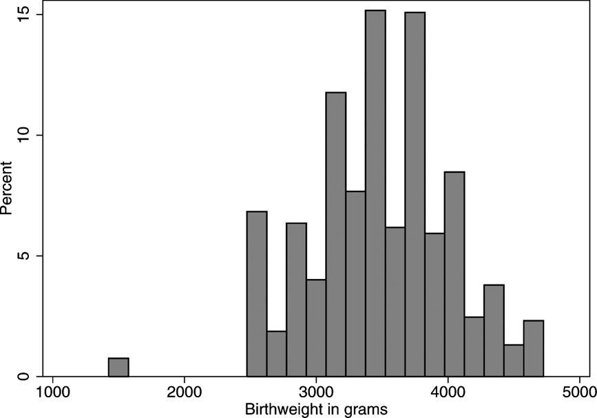
For the vast majority of subjects in the sample (over 99%), the responses were provided by the biological mother. In this study those subjects where the answer was not provided by the biological mother were dropped, as were non-singleton births. The principal dependent variable used in this study is the birth weight of the child. Birth weight is recorded in the survey in intervals of 100 g and there is data censoring at both the top and bottom of the distribution. All birth weights in excess of 4600 g are listed as 4600 g. Meanwhile all birth weights below 1499 g are listed as 1499 g. In addition, birth weights in the 1500–2499 g interval are simply listed as 2499 g. The histogram for birth weight is provided in Fig. 1. Given the data censoring referred to above, the slight heaping evident at 1499 and 2499 g is to be expected. Given this censoring of the data, LBW must be analysed as a binary rather than continuous variable. However, as explained above, this is also desirable according to the principle of focus. After adjusting for sampling weight, the rate of LBW is about 5.8%. This is somewhat higher than the rate reported in the Irish perinatal statistics of 2009, which lists 3.7% of live, singleton births as being less than 2500 g (Economic and Social Research Institute, 2011).

Fig. 1. Histogram of birth weights, GUI survey (N=10,196).
As pointed out by Kramer et al. (Reference Kramer, Seguin, Lydon and Goulet2000), LBW is in some respects an unsatisfactory outcome for epidemiological analysis, since birth weight may be determined by both duration of gestation and by the rate of fetal growth. Thus LBW may occur either because an infant is born too early (a preterm birth) or because it is small for his/her gestational age (this can be regarded as a case of intrauterine growth restriction, IUGR). This distinction is of particular importance since evidence suggests that the determinants of gestational duration (and hence the issue of preterm) may be quite different from those of IUGR (see Kramer et al., Reference Kramer, Seguin, Lydon and Goulet2000, and the references therein). This in turn may imply a different socioeconomic gradient for preterm compared with IUGR. It may also have consequences for the decomposition of the concentration index outlined above, as the relative contribution of each factor to the concentration index may differ between overall LBW, preterm and IUGR.
A distinction is made between preterm and cases of IUGR in the following way. In addition to answering questions about birth weight, subjects are also asked after how many weeks of pregnancy the baby was born. All those answering less than 37 weeks are defined as preterm. The IUGR cases are then defined as those that are LBW but not preterm. For the sake of comparison analysis is carried out for overall LBW, preterm and IUGR (analysis is also carried out using a lower cut-off of 32 weeks; results available on request).
Household resources
The particular measure of household resources used to calculate the concentration index is equivalised net income. Net income is the response to a question asking for the net income of all household members. It is defined as total gross household income less statutory deductions of income tax and social insurance contributions. It is then equivalised by dividing by the square root of household size.
Of course, the expectation is that LBW would also be correlated with other measures of socioeconomic status such as education or class. However, as these are not cardinal variables it is not possible to calculate concentration indices with respect to these variables. However, the education levels of both parents are included as explanatory variables in the decomposition of the concentration curve.
Summary statistics
Before providing results regarding the concentration curve and the contribution of various covariates, some summary statistics for overall birth weight (bearing in mind that the data are censored at either end), LBW, preterm and IUGR are presented. In Tables 1 and 2 the data for all observations are presented, as well as by mother's education and social class and household income quintile. Education is divided into five categories: lower secondary (i.e. left school before age 17/18), leaving certificate (completed secondary school education), diploma/certificate (Dip/Cert) (obtained qualification after secondary school but did not go on to tertiary level education), tertiary level education and postgraduate education. Social class is divided into three categories, according to those provided in the survey (professional/managerial; non-manual and skilled manual; semi-skilled and unskilled manual) and then a fourth group listed as ‘never worked at all, no class’.
Table 1. Summary birth weight statistics, GUI survey (N=10,196)

Table 2. Low birth weight by mother's education, household income and social class, GUI survey (N=10,196)

The socioeconomic gradient is evident in pretty much all cases, but it is more pronounced in some cases compared with others. In particular, the prevalence of LBW and IUGR is concentrated amongst the ‘lowest’ of the groups. For example, in the case of IUGR by social class there is little evidence of a gradient for three of the classes (with incidence in a narrow range between 1.8% and 2%) and then a jump to 4% for the ‘never worked/no class’ group. This differential gradient by socioeconomic class and by measure of LBW suggests a significant role for confounding factors and these are examined when decomposing the concentration index.
Missing observations
Before presenting results there is a specific data issue that must be addressed. In calculating the concentration indices and in providing the decomposition, it must be borne in mind that some observations are missing, and in particular it is possible that such observations may not be missing at random. Compared with the base sample size of 10,969 there are over 800 observations where income data are missing. When account is taken of the right-hand-side variables used for the decomposition approximately another 670 observations are lost. There are a variety of approaches one can take when faced with missing data (see Horton & Kleinman, Reference Horton and Kleinman2007). One possibility is to adopt the ‘complete-case’ approach, using only those observations with no missing values for any variable. This gives a sample size of 9469. The concentration indices for LBW, preterm and IUGR calculated using this sample are −0.434, −0.410 and −0.516 respectively.
However, the complete-case approach can be regarded as overly ad hoc as a means to address missing data. Since the variable with the greatest number of missing observations is income, and since income is critical in terms of calculating concentration indices, it seems worthwhile to try to deal explicitly with the missing values for this variable at least. One possible way of doing this is to estimate an income function, by regressing equivalised income on age and education. One can then substitute the fitted values from this regression for those observations where income is missing. This provides a sample size of 10,196. The concentration indices calculated for this sample are −0.461, −0.411 and −0.511. This is known as the regression prediction or conditional mean imputation approach (where it is applied to income only). While there are some differences from the indices calculated using the complete-case approach, they are of a similar order of magnitude suggesting that the missing observations do not unduly bias the results. Note that missing observations for variables other than income are only relevant when carrying out the decomposition. It is possible to calculate concentration indices only using the conditional mean approach, which would give a full sample of 10,969 (giving values of −0.476, −0.470 and −0.461). However, in this case, it would not be possible to carry out the decomposition. Thus the approach adopted could be characterized as a combination of the complete-case approach with conditional mean imputation applied to the income variable.
Variables for decomposition
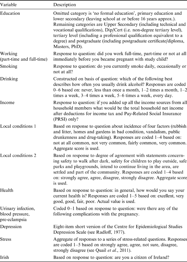
The choice of right-hand-side variables for the decomposition of the concentration indices is influenced by the review by Kramer et al. (Reference Kramer, Seguin, Lydon and Goulet2000) and of course by data availability. The variables chosen are: age of mother and age squared (to allow for a non-linear effect), sex of child (male children are typically heavier at birth), education of both parents, working status of mother, mother's smoking and drinking, body mass index (BMI) of mother and BMI squared, log of disposable household income, two measures reflecting local environmental conditions, general health of mother plus information on some specific conditions (mental and physical) and ethnicity of mother (Irish or non-Irish). Full details of all explanatory variables are provided in the Appendix Table A2.
Results
Concentration indices
Table 3 provides concentration indices for LBW, preterm and IUGR. All indices are negative and in the −0.4 to −0.5 region, indicating that the incidence of the phenomenon in question is substantially concentrated amongst the less well-off. In all cases the p-values are less than 0.05 and the values of the concentration index do not appear to be unduly sensitive to the way in which the missing observations are treated.
Table 3. Concentration indices for various measures of low birth weight, GUI survey (N=10,196)

Before analysing the decomposition of this index, it is useful to try to get an intuitive sense of what these figures actually mean. The sign of the concentration index indicates the direction of any relationship between the health variable and rank in the distribution of whatever measure of household resources is being used. The magnitude reflects both the strength of the relationship and the degree of variability in the health variable. In addition, Koolman & Van Doorslaer (Reference Koolman and Van Doorslaer2004) have shown that multiplying the value of the index by 75 gives the percentage of the ill-health variable which, in the case of a negative index, would need to be redistributed from the poorer half to the richer half of the population to arrive at a distribution with an index of zero.
Decomposition
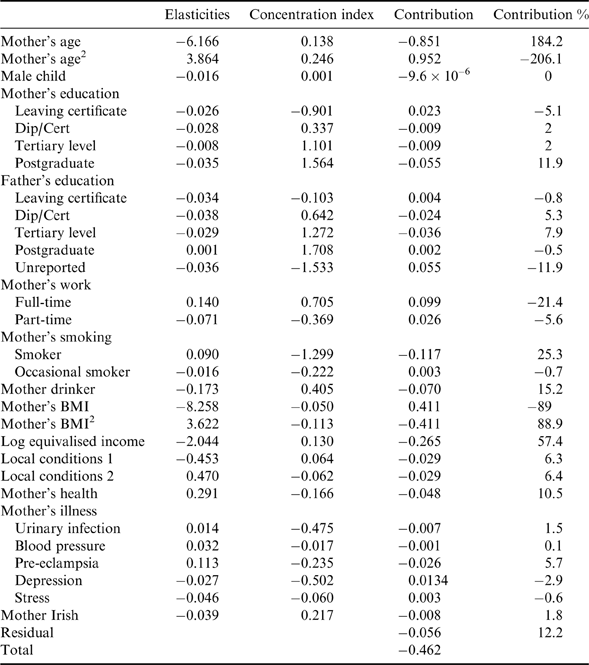
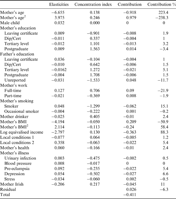
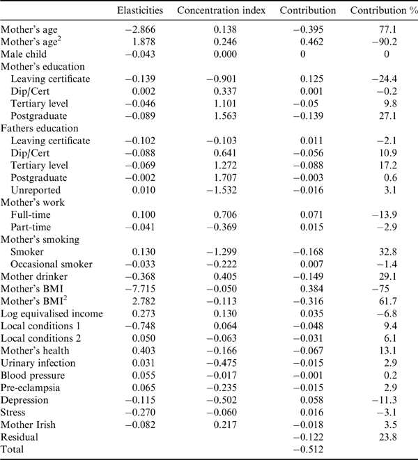
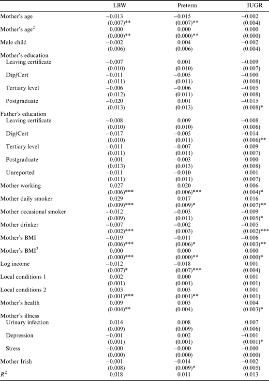
We now turn to the decomposition results in Tables 4–6 (note that the regressions underlying these decompositions are provided in Table A1). Perhaps the first issue to note is that the right-hand-side variables explain a considerable portion of the income-related inequality, ranging from over 100% in the case of preterm to about 75% in the case of IUGR. Recall that in order for any variable to contribute to income-related inequality it must (a) influence the measure of LBW (which can be examined via the elasticities column) and also (b) itself be related to the distribution of income (which can be examined via the value of its own concentration index). Note also that variables can contribute both positively and negatively to the overall concentration index. In the discussion that follows it is important to bear in mind that the overall concentration index for all measures of LBW is negative, i.e. it is more concentrated amongst the less well-off. The column labelled ‘Contribution %’ shows the percentage contribution of each factor to overall income-related inequality in LBW. A positive value indicates that this factor operated to bring about the concentration of LBW amongst the less well-off. A negative value indicates that the factor operated in the opposite direction, i.e. on its own, this factor would have led to LBW being more concentrated amongst the better-off.
Table 4. Decomposition of concentration indices, low birth weight, GUI survey (N=10,196)

Table 5. Decomposition of concentration indices, preterm, GUI survey (N=10,196)

Table 6. Decomposition of concentration indices, IUGR, GUI survey (N=10,196)

Bearing this in mind it can be seen in Table 4 that the most important factors with respect to overall LBW, in absolute terms, were mother's age, working status, smoking, drinking and overall health and household income. The contributions of age and age squared can be combined to arrive at a contribution of −22%. The regression results show that incidence of LBW first of all declines with age, bottoms out at about 27 and then rises with age. The concentration curve for age is positive, though relatively low (i.e. older mothers are better off on average than younger mothers, but not by an awful lot). Combining all these factors together, the impact of mother's age, on its own, is to increase the incidence of LBW amongst the better-off.
The mother working full-time and part-time also make substantial negative contributions to the overall concentration index, to the tune of about −27%. Bonzini et al. (Reference Bonzini, Coggon and Palmer2007), in a review of the evidence concerning working and a number of adverse birth outcomes (including preterm delivery and LBW), suggested that for preterm delivery there was extensive evidence of an effect of certain occupational exposures, viz. long working hours, shift-work, lifting, standing and heavy workload. The findings in Tables 4–6 partially confirm this in that greater effects are observed for overall LBW and preterm than for IUGR. Given that working is associated with a greater likelihood of LBW, and given that it is also associated with higher incomes, the combined effect is that working tends to increase the concentration of LBW amongst the better-off and hence makes a negative contribution to the concentration index.
Smoking makes one of the largest positive contributions to the concentration index. In this case the pathway appears clear. Smoking is associated with LBW and is heavily concentrated amongst lower income mothers (see Kramer et al., Reference Kramer, Seguin, Lydon and Goulet2000) and the combination of these factors implies that it makes a contribution of about 25% to the concentration index.
What is perhaps slightly more surprising is that drinking alcohol also contributes positively (just over 15%) to the concentration index. Drinking is concentrated amongst better-off mothers and LBW has an elasticity of −0.173 with respect to drinking. Unfortunately, the data do not provide information on drinking behaviour during pregnancy, but rather drinking behaviour at time of interview. However, it is worth noting that the negative relationship between alcohol consumption and LBW is also found in the 9-year cohort of the GUI survey and in that instance alcohol refers to alcohol consumption during pregnancy.
The biggest single contributor to the negative concentration index for LBW is income itself (to be more precise, the log of equivalised income). While it may seem strange that income should be a right-hand variable in this decomposition, perhaps the easiest way to view this is to consider what the gradient would be if everyone had the same income. In this case there clearly could be no gradient, in the sense of a relationship between LBW and income, since everyone would have the same income. Correspondingly, if LBW is negatively related to income, then any factor that leads to a widening of income inequality will increase the (negative) value of the concentration index.
The final variable that makes a substantive contribution to the negative concentration index is mother's overall health. As in the case of smoking, the pathway appears reasonably straightforward. Poorer overall health increases the probability of LBW, and since there is a well-documented gradient between health and income (e.g. Kakwani et al., Reference Kakwani, Wagstaff and Van Doorslaer1997) this translates into a contribution of over 10% to the concentration index.
Tables 5–6 show a similar decomposition for preterm and IUGR. The breakdown for preterm is quite similar to that for overall LBW, with one or two exceptions. The contributions of mothers' smoking and drinking are less, while income makes a substantially greater contribution in the case of preterm, with a considerably higher elasticity.
Table 6 shows the breakdown for IUGR, and here greater differences with respect to overall LBW are observed. The residual element is larger here, with nearly one-quarter of the total concentration index unexplained. Looking at the individual variables, father's education exercises a greater role, with the sum of these variables contributing nearly 30% to the index. There is a much diminished role for income per se. Compared with a contribution of 58% for overall LBW it now contributes only −6.8%, i.e. IUGR is positively related to income, though the effect is small. There is also a greater role for local environmental and health variables.
Characteristics and returns to characteristics
The approach adopted so far has assumed that socioeconomic inequality in the various forms of LBW arises from difference in characteristics only. An alternative way to express this is that in the regression-based decomposition, it is assumed that the effect of each covariate on LBW is common across all levels of income. However, this may not be the case. For example, it is possible that the effect of ill health on LBW may differ by income level. This could arise because richer mothers may have the resources to partially offset the effects of ill health. Thus at a more general level it is possible that differing LBW by income level may arise owing to different characteristics and/or different returns to these characteristics (i.e. the returns differ by income).
This is explored using a variant of the well-known Blinder–Oaxaca decomposition (see Blinder, Reference Blinder1973; Oaxaca, Reference Oaxaca1973) whereby, in this case, it is necessary to partition the sample into two groups by income. They are partitioned according to median equivalised income into the ‘rich’ and ‘poor’ (a partition at the 25th percentile into the ‘very poor’ and the rest is also used). The overall gap in LBW between the two groups will then be decomposed into a part arising from differences in characteristics and differences in returns to characteristics (i.e. the impact of these characteristics on LBW). The results are presented in Table 7 and indicate that for all forms of LBW and for both the poor–rich and very poor–rich partitions, around 90% (in some cases more) of the gap is explained by differences in characteristics, rather than returns to characteristics.
Table 7. Blinder–Oaxaca decomposition of LBW gap (%), GUI survey (N=10,196)

Discussion
Limitations
It is perhaps useful to discuss some possible limitations of the study's approach. First, one of the limitations of the approach adopted here is the use of a summary index. A summary index does have the advantage of presenting results in a clear and simple way, and in a manner in which it is straightforward to make comparisons across countries/regions and time. However, summary indices by their nature also conceal detail. For example, the use of the simple concentration index does not permit a higher weighting to be put on babies with very low birth weight, i.e. less than 2000 or 1500 g. When using continuous data it is possible to employ extended concentration indices, which do have this property (see Wagstaff, Reference Wagstaff2002). However, as explained above, when analysing LBW, owing to the principle of focus it appears preferable to adopt a binary approach.
A further limitation of the approach here is the presence of a residual in the decomposition of the concentration index. This arises because the concentration index does not provide an exact decomposition, in the sense that the value for the index will exactly equal the sum of the contributions from the covariates. This is a standard property of rank-based indices such as the Gini coefficient. However, it is reassuring to note that for the decompositions calculated here, the residual is comparatively small.
As for limitations arising from the data employed, the Growing Up in Ireland survey is a comprehensive, nationally representative survey of a 9-month-old cohort of children. However, birth weight data are supplied retrospectively by the mother, and so they may be prone to some measurement error. The comparatively high rate of LBW compared with the 2009 perinatal statistics suggests that this may be an issue. However, given that the study did not attempt to measure LBW per se but merely how it relates to socioeconomic status, this is only a cause for concern if the measurement error is correlated with such status. When a lower threshold is used for low birth weight (1500 g) it is found that the concentration index is around −0.4, qualitatively very similar to the 2500 g threshold, though given that numbers of children with birth weight less than 1500 g is very small, this index is less precisely measured (results available on request). The result, however, is reassuring since it suggests that the value of the concentration index is not too sensitive to the precise location of the cut-off and so even if there is some measurement error around the 2500 g cut-off it is unlikely to appreciably affect the results.
Finally, as noted above, there are a number of missing observations, partly owing to missing income data and partly owing to some missing data for the covariates in the decomposition. However, as discussed above, the calculated concentration indices all appear to be in the region of −0.4 or −0.5 regardless of how the missing data issue is treated and also regardless of the inclusion or otherwise of those observations that were dropped because data were missing for one of the decomposition covariates. Thus overall, the fundamental results obtained in the paper do not appear to be unduly sensitive to the limitations discussed.
Summary and conclusion
Socioeconomic inequalities in health entail inferior health outcomes for lower income groups, which in turn have effects on quality of life and labour market outcomes. There is considerable evidence that early life conditions have a significant impact on later life health outcomes; hence it is likely that socioeconomic inequalities in these early life conditions will have persistent effects. To that extent, careful measurement of such inequalities for low birth weight, one of the most salient manifestations of poor early life health conditions, may provide valuable policy insights to address later inequalities.
This paper has provided a new perspective on the issue of socioeconomic inequalities for low birth weight in Ireland by calculating concentration indices, the standard summary measure of socioeconomic inequality, for a representative sample of births. A further innovation of the paper is that the indices are calculated for LBW arising from two different sources: preterm and intrauterine growth retardation. For all forms of LBW the calculated concentration indices are in the −0.4 to −0.5 region, indicating fairly substantial concentration amongst the less well-off.
This paper also provides a decomposition of the concentration index. While not implying causality this decomposition provides an insight into which socioeconomic, lifestyle and demographic characteristics are associated with LBW, with evidence provided for both sources. In turn these results can direct policy that may redress these inequalities.
The decompositions of the concentration index for the different sources of low birth weight show some uniformity, but there are also some differences. For example, income inequality appears to be less important for the case of preterm births, while father's education and local environmental conditions appear to be more relevant for IUGR.
Finally, the paper applies the standard Blinder–Oaxaca decomposition to investigate the degree to which the socioeconomic gradient for all sources of LBW arise owing to the different characteristics of rich and poor or instead to the effect of these characteristics on LBW. The evidence indicates that it is differences in characteristics as opposed to the impact of these characteristics on LBW that is the principal source of the socioeconomic inequalities.
Acknowledgments
The author thanks the Irish Social Science Data Archive for making the Growing Up in Ireland data available. He would also like to thank Brian Nolan and an anonymous referee for helpful discussion and comments. The usual disclaimer applies. The author declares that there was no personal or financial conflict of interest involved in the preparation of this manuscript.
Appendix
Table A1. Low birth weight regressions (N=10,196), with robust standard errors in parentheses

Table A2. List of variables used for decomposition


