


Introduction
Human populations tend to depart from the equilibrium conditions predicted by the Hardy–Weinberg law, so that mating in finite populations is not always random and individuals have some consanguinity. Studies on extended genomes in different populations have demonstrated the existence of significant portions of homozygosis (>4Mb) in subjects with no known consanguineous unions in their genealogies in the past five to ten generations (Li et al., Reference Li, Ho, Chen, Wei, Wong and Li2006; Simon-Sanchez et al., Reference Simon-Sanchez, Scholz, Fung, Matarin, Hernandez and Gibbs2007; McQuillan et al., Reference McQuillan, Leutenegger, Abdel-Rahman, Franklin, Pericic and Barac-Lauc2008).
It has been estimated that 690 million individuals worldwide are consanguineous (Bittles, Reference Bittles2010; Bittles & Black, Reference Bittles and Black2010; Denic et al., Reference Denic, Naglekerke and Agarwal2011). However, according to Bittles (Reference Bittles2005), although considerable attention is paid to the role of consanguinity as a causal factor of genetic disorders, the potential influence of population endogamy on the overall levels of homozygosis remains underestimated.
There are strong indications that in the Arab world consanguineous marriages are more common in the lower socioeconomic strata and are negatively associated with modernization, literacy and urbanization indicators (Bittles, Reference Bittles1994; Khlat, Reference Khlat1997). Infant mortality rate, one of the most important indicators of the socioeconomic and health status of a community, shows a strong and positive relation with consanguinity (Kerkeni et al., Reference Kerkeni, Monastiri, Guediche and Ben Cheikh2007; Weinreb, Reference Weinreb2008; Abuqamar et al., Reference Abuqamar, Coomans and Louckx2011). However, the association of lower socioeconomic strata with consanguinity is not unique to the Arab world, as demonstrated by a study carried out in Jerusalem where more than half of the population under study were descended from Mizrahi and Sephardic Jews and the rest came from Western Asia, North Africa and Europe (Harlap et al., Reference Harlap, Kleinhaus, Perrin, Calderon-Margalit, Paltiel and Deutsch2008).
The relationship of consanguinity with social, economic and political issues has recently received a great deal of interest (d’Alpoim Guede et al., Reference d’Alpoim Guede, Bestor, Carrasco, Flad, Fosse and Herzfeld2013) based on the works of Bildirici et al. (Reference Bildirici, Kὄkdener and Ersin2010), Ashraf and Galor (Reference Ashraf and Galor2013) and Woodley and Bell (Reference Woodley and Bell2013). Bildirici et al. (Reference Bildirici, Kὄkdener and Ersin2010) showed that countries reaching high development levels, as measured by their Gross Domestic Product, have a lower frequency of consanguineous marriages. Ashraf and Galor (Reference Ashraf and Galor2013) related the genetic diversity of populations to economic development. Finally, Woodley and Bell (Reference Woodley and Bell2013) suggested that development of democracy is negatively associated with consanguinity and that this relationship can be used as a predictor of the level of democratization reached by nations.
Consanguinity in a population can be estimated by three methods, based on genealogic, genomic or surname information, each with their advantages and limitations. The advantage of the use of surnames (the isonymic method), compared with the use of genealogies and molecular information, is that it allows, at very low cost, a diagnosis of consanguinity for the entire population when using appropriate information sources (e.g. electoral rolls) (Scapoli et al., Reference Scapoli, Mammolini, Carrieri, Rodriguez-Larralde and Barrai2007). In recent years a number of important isonymic studies at continent, country, province or state, regional and city level have been published, mainly due to the accessibility of various sources of large numbers of surnames in digitalized format (see, for example, Lasker, Reference Lasker1985; Colantonio et al., Reference Colantonio, Lasker, Kaplan and Fuster2003; Scapoli et al., Reference Scapoli, Mammolini, Carrieri, Rodriguez-Larralde and Barrai2007; Bronberg et al., Reference Bronberg, Dipierri, Alfaro, Barrai, Rodríguez-Larralde and Castilla2009; Rodriguez-Larralde et al., Reference Rodriguez-Larralde, Dipierri, Alfaro, Scapoli, Mamolini and Salvatorelli2011).
The possibility of describing consanguinity, in relative terms, by the isonymic method at any level of the political–administrative structure of a nation, makes it an additional and highly informative demographic variable (Bittles, Reference Bittles1994; Dipierri, Reference Dipierri2014) that can be related to others of a biological and/or sociocultural nature.
This study examined the relationship of consanguinity by random isonymy (F ST) with socioeconomic status at different levels of organization in Argentina. This approach is based on the fact that various flexible, labile and interdependent genetic, demographic and social structures co-exist in human populations (Macbeth & Collison, Reference Macbeth and Collison2002), and that clustering patterns, generally responding to a hierarchical ordering (Harrison & Boyce, Reference Harrison and Boyce1972), can be described in each of these structures.
Methods
To estimate F ST, the surnames of 22.6 million individuals registered in the 2001 Argentine Electoral Roll, corresponding to individuals older than 18 years, representing approximately 60% of the population, were used. Administratively Argentina is composed of five geographic regions, each of which is in turn formed by a variable number of provinces and these by departments, which total 510. Thus Argentina can be divided into the following regions: Region 1 (Central) with the Autonomous City of Buenos Aires (CABA) and the provinces of Buenos Aires, Santa Fe, Cordoba, Entre Rios and La Pampa; Region 2 (Patagonia), with the provinces of Neuquen, Chubut, Rio Negro, Santa Cruz and Tierra del Fuego; Region 3 (NOA, Argentine North-West), including the provinces of Catamarca, Tucuman, Salta, Jujuy, Santiago del Estero and La Rioja; Region 4 (Cuyo), with the provinces San Luis, San Juan and Mendoza; and Region 5 (NEA Argentine North-East) with the provinces of Chaco, Corrientes, Formosa and Misiones (Fig. 1). The analysis was performed for the nation as a unit and for each of the five geographic regions.
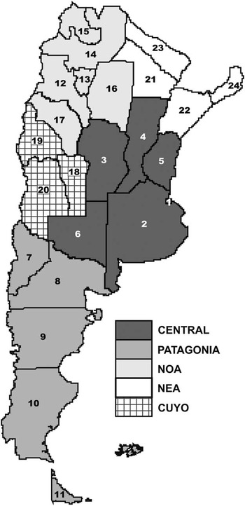
Fig. 1 Regions and provinces of Argentina. Region Central: 1. Ciudad Autonoma de Buenos Aires (CABA), 2. Buenos Aires, 3. Cordoba, 4. Santa Fe, 5. Entre Rios y 6. La Pampa; Region Patagonia: 7. Neuquen, 8. Chubut, 9. Rio Negro, 10. Santa Cruz y 11. Tierra del Fuego; Region NOA: 12. Catamarca, 13. Tucuman, 14. Salta, 15. Jujuy, 16. Santiago del Estero y 17. La Rioja; Region Cuyo: 18. San Luis, 19. San Juan y 20. Mendoza; Region NEA: 21. Chaco, 22. Corrientes, 23. Formosa y 24. Misiones.
The isonymic variable (FST)
Crow and Mange (Reference Crow and Mange1965) noted the ongoing relationship between the probability of spouses having the same surname (isonymy, I) and the coefficient of consanguinity of the offspring (F), such that I/F equals 4 in most of the common marriage relationships. In the hierarchical model of consanguinity (Wright, Reference Wright1951), founder and descendant populations are related by a branching process. The consanguinity coefficient relative to the overall population is F IT; the departure from panmixia within a descendant population is measured by F IS; the divergence of a descendant population from a founder population is measured by F ST, or random isonymy (Barrai, Reference Barrai1971). A large value of F ST would then indicate large consanguinity and drift, whereas a small value would indicate migration and low consanguinity. Further theoretical and methodological details concerning the calculation of F ST are available in Relethford (Reference Relethford1988).
The Socio-Demographic and Economic Indicator (SDEI)
Information regarding socio-demographic and socioeconomic variables came from the 2001 Census of Population and Housing (INDEC, 2001) and the Department of Health Statistics and Information, Argentine Ministry of Health. The following types of variables were considered: education, economy, health, unsatisfied basic needs and infant mortality. Using a principal component analysis a Socio-Demographic and Economic Indicator (SDEI) was computed, which summarizes the effect of socioeconomic and demographic variables at the departmental level. The SDEI may be considered an indicator of educational, economic, labour and health opportunities. It is a measurement of development or deprivation, with high SDEI values denoting more development and less deprivation. In Argentina, this value ranges from 6.71 in the Autonomous City of Buenos Aires (Central Region), down to −3.90 in the province of Formosa (NEA Region). Further details on the calculation of SDEI are available in Bronberg et al. (Reference Bronberg, Gutiérrez Redomero, Alonso and Dipierri2012).
Statistical analysis
The relationship between departmental F ST as dependent variable and departmental SDEI as the independent one was established by multiple regression analysis, according to a linear model, for the whole nation and by region. A statistical description by regions of F ST and SDEI was performed including the estimation of mean, standard deviation and extreme values. Using a non-parametric analysis with the Kruskal–Wallis test, relevant F ST and SDEI comparisons were performed. Standard statistical software was used (Statgraphics and Statistica).
Results
Table 1 shows the descriptive statistical values for F ST and SDEI by region. Significant differences for the medians of F ST and SDEI between regions (p<0.05) were confirmed by the Kruskal–Wallis test. Mean F ST values showed the following regional gradient: Central was lower than Patagonia, which was lower than Cuyo, which equalled NEA, and these were lower than NOA. The order for mean SDEI was: NEA was lower than NOA, which was lower than Cuyo, which equalled Patagonia, and these were lower than Central.
Table 1 F ST and SDEI values by region, Argentinian electoral roll
The regression between the SDEI and F ST log-transformation was calculated for the whole country, using 510 points (departments). The equation obtained was:
 $${\rm log}\,\left( {F_{{{\rm ST}}} } \right)\,{\equals}\,{\minus}6.90079{\minus}0.185194{\rm {\times}SDEI,}$$
with a significant regression coefficient (Fig. 2). The correlation was negative and statistically significant (r=−0.678693, p≤0.0001). The value of r 2 indicates that SDEI explains 46% of the variability of log(F ST) in Argentina. The corresponding regression equations for each region are shown in Fig. 3. The regression coefficients by region were significantly different (p<0.001), with the highest slope in the Central region and the lowest in the NEA and NOA regions. The correlations of F ST with SDEI by region were also negative and statistically significant, showing the highest r value in the Central region, followed by Patagonia, Cuyo, NEA and NOA (Table 2).
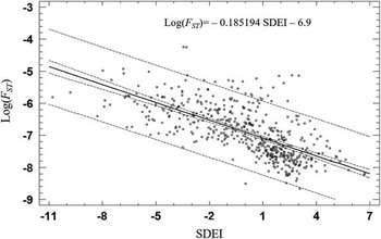
Fig. 2 Regression of log(F ST) on SDEI based on 510 points, with 95% confidence intervals.

Fig. 3 Linear regression of log(F ST) on SDEI, by region.
Table 2 Correlation (r) and linear regression of log(F ST) on SDEI by region, Argentinian electoral roll
*p<0.03.
Figure 4 presents a scatter plot of F ST and SDEI by latitude and longitude, where each point represents the corresponding values for a department. In the north of the country high F ST and low SDEI values were found, while in the south the opposite tended to be found. Some exceptions were observed in NOA, where a few highly developed departments were found.

Fig. 4 Bubble scatter plots showing SDEI and F ST by longitude and latitude. Each department is represented by a bubble, the size of which corresponds to the values of SDEI (a) or F ST (b).
Discussion
There have been very few studies on the relationship between consanguinity by random isonymy and socioeconomic status (Sawchuk & Herring, Reference Sawchuk and Herring1989; Little & Malina, Reference Little and Malina2005; Guell et al., Reference Guell, Rodríguez Mora and Telmer2007; Collado et al., Reference Collado, Ortuño Ortiz and Romeo2008; Bronberg et al., Reference Bronberg, Dipierri, Alfaro, Barrai, Rodríguez-Larralde and Castilla2009; Kiranmala et al., Reference Kiranmala, Asghar and Saraswathy2011), and even fewer have been at the national level. Most of these studies agree that high consanguinity, as estimated by isonymy, occurs predominantly in economically disadvantaged communities.
Previous studies have indicated that the Argentine isonymic structure as revealed by F ST exhibits a marked regional and departmental variation, showing the highest values towards the north and west of the country (Dipierri et al., Reference Dipierri, Rodríguez-Larralde, Barrai, López-Camelo, Gutierrez-Redomero and Rodríguez2014). The F ST has been found to be highest in La Rioja, Corrientes and Santiago del Estero, which are provinces in the north, and lowest in the area of Buenos Aires and the province of Santa Fe, both in the central portion of the country (Dipierri et al., Reference Dipierri, Alfaro, Scapoli, Mamolini, Rodríguez-Larralde and Barrai2005).
Among the demographic factors that affect the structure of consanguinity of the present population in Argentina, size and migration can be identified. Population size affects the estimates of F ST in regions, provinces and communes, and for the country as a whole, when different subdivisions are considered. It constitutes the ‘Prefecture Effect’, so named by Scapoli et al. (Reference Scapoli, Mammolini, Carrieri, Rodriguez-Larralde and Barrai2007). This effect for F ST was described in Japan by Nei and Imaizumi (Reference Nei and Imaizumi1966). They observed that, for the same area and population, small subdivisions have larger F ST values, and larger subdivisions have smaller F ST values. In their study, the effect was seen in towns and in the prefectures where the towns were located, hence the name.
The size of the 2001 Argentinian departmental electoral roll is positively correlated with latitude and negatively with longitude, indicating a spatial dispersion in Argentina, which is the opposite to that of consanguinity by random isonymy (Dipierri et al., Reference Dipierri, Rodríguez-Larralde, Barrai, López-Camelo, Gutierrez-Redomero and Rodríguez2014). The departments with the largest population size tend to be located to the centre of the country. Moreover, F ST was negatively correlated with the population size of the electoral roll (r=−0.168; p<0.0001). In Argentina, according to the 2001 National Census (INDEC, 2001), the provinces of Buenos Aires, Córdoba, Santa Fe and Buenos Aires Autonomous City, located in the Central Region, concentrate 62.51% of the total population of the country in 606,102 km2, with a population density of 37.4 inhabitants/km2, against a density of 13 inhabitants/km2 for the whole country. The rest of the Argentine population (37.5%) is located in the remaining 2,174,102 km2.
With allochthonous migrations from Europe between 1870 and 1929, the main contributions to Argentine onomastics occurred with surnames of European (non-Spanish) or Asian geographical and/or linguistic origin, which caused greater diversity of surnames in the south. According to Lattes and Recchini de Lattes (Reference Lattes and Recchini de Lattes1994), about 5.3 million migrants entered from the late nineteenth century until 1970. However, the distribution of these migrants in the vast Argentine territory was not uniform. According to the National Census of 1914 (DEyC-Corrientes, 2014), which coincides with the period of increased immigration, the highest percentage of the total national non-native population was located in the Central region (87.4%), followed by Cuyo (4.9%), NOA (3.1%), NEA (2.7%) and Patagonia (2%) (Benencia et al., Reference Benencia, Devoto, Míguez, Moreno and Nabel2003; Girbal de Blacha, Reference Girbal de Blacha2003). The spatial distribution of the non-native population matches F ST, showing that immigrants tend to be preferentially located in departments and regions of the less isolated and more economically developed south-east. The continental allochthonous migrations occurred through all the borders connecting Argentina with Bolivia and Paraguay in the north, Chile in the west and Uruguay and Brazil in the east. But overall, these migrants tended to stay in the border provinces or in the Autonomous City of Buenos Aires. In this case, the contribution to the diversity of surnames was scarce because the geographic-linguistic origin of most of these migrant surnames was Spanish, except for those who came from Brazil. Migratory demographics also coincided with the distribution of Fisher’s α (Fisher et al., Reference Fisher, Corbet and Williams1943) at the departmental level: high in the east and lower in the west of the country (Dipierri et al., Reference Dipierri, Alfaro, Scapoli, Mamolini, Rodríguez-Larralde and Barrai2005). The distribution of this indicator was consistent with the settlement of subsequent waves of immigrants in the 20th century, moving from the North Atlantic coast towards the foot of the Andes and towards the south, indicative that migration in Argentina dominated over drift (Dipierri et al., Reference Dipierri, Alfaro, Scapoli, Mamolini, Rodríguez-Larralde and Barrai2005).
The literature on Argentine demographic and socioeconomic structure is abundant and has shown that socioeconomic phenomena (unemployment, economic inequality and welfare, etc.) have been characterized by their discriminative spatial character. Gasparini et al. (Reference Gasparini, Marchionni and Sosa Escudero2003) applied the Gini coefficient to assess income inequality in the major urban centres of the country in the Permanent Household Survey, conducted between the years 1997 and 1999 (INDEC, 2000). From this survey the percentage of the population below the poverty line (theoretical income necessary to meet the minimum requirements of quality of life of a person or household in a given country) can also be estimated. The Material Deprivation Index Survey (INDEC, 2003) allows simultaneously recognition of poor households and characterization of the heterogeneity and intensity of deprivation situations. From all these sources of information, NOA and NEA have been the poorest regions in the country; the Central region, and especially Patagonia, have poverty levels below the national average (Gasparini et al., Reference Gasparini, Marchionni and Sosa Escudero2003), with a distribution matching F ST and opposite to that of ISDE.
Although censuses are inadequate to measure the magnitude of consanguinity, they still collect data based on blood ties, marriage or friendship among people who share space and collectively organize to survive, so they can indirectly provide information on kinship and distribution of surnames. The group census information refers to the household or domestic unit census, defined as a person (individual) or group of persons (multi-person), related or not, living under the same roof and generally sharing food. Social factors (unemployment, separation, widowhood and migration) place consanguineous family members in situations of forced co-existence. Crises linked to economic and marital situations determine that the most impoverished and vulnerable families reorganize in the same household. On the other hand, there are single-person households, for those who have had economic benefits, which enables them to organize independently, away from the patriarchal structure formed by the multi-person household centred on a householder. In Argentina, the complete nuclear household (a couple with or without children) is predominant, followed by extended families (parents and children and other relatives) and composite households (including non-relatives). The presence of extended families, especially in the poorest sectors, is interpreted primarily as a response to economic adversity, since the presence of additional members can be a valuable help to increase family income or perform household chores (Ariza & De Oliveira, Reference Ariza and De Oliveira2001). Single-person households prevail in the more developed regions (Central and Patagonia), while multi-person households and overcrowding are more prevalent in NOA and NEA (Dipierri, Reference Dipierri2014). On the assumption that the repetition of the same surname is more likely in multi-person households, this might partially explain the higher values of F ST observed in populations of northern Argentina, which happen to be the most impoverished in the country. On the other hand, the differences found between the regional regression lines of log(F ST) on SDEI (Fig. 3) can be partially explained because NOA and NEA, with the lowest slopes, are the regions where F ST tends to be above the predicted values for a given SDEI in most departments, while in Central and Cuyo, more variability in both variables and a better adjustment between observed and predicted values is observed.
A series of papers from the field of economics contribute to understand the relationship between surnames, consanguinity and socioeconomic factors. These studies have suggested that information on inter-generational mobility becomes available by the simultaneous observation of the frequency and distribution of surnames and income of a society. According to Guell et al. (Reference Guell, Rodríguez Mora and Telmer2007), in Western societies the distribution of surnames is uneven, as relatively common surnames co-exist with rare surnames carried by a variable percentage of the population. These rare surnames are the main source of information to analyse inter-generational mobility. Guell et al. (Reference Guell, Rodríguez Mora and Telmer2007) characterized the joint distribution of surnames and income and analysed the correlation between social mobility and the informative content of surnames in the Catalan population, showing that these contained financial information. There was a negative relationship between the frequency of surnames and socioeconomic status, so in the Catalan population the richest people had less-common surnames. Collado et al. (Reference Collado, Ortuño Ortiz and Romeo2008) studied the association between surnames from the phone book and socioeconomic status of the Spanish population and arrived at a similar conclusion.
In short, from the relations established in this study between consanguinity by random isonymy and SDEI it can be concluded that the most isolated, inbred and impoverished departments of Argentina tend to be located in the north, and the more developed, less impoverished and less inbred regions tend to be in the centre and south of the country. This study has therefore verified a statistically significant inverse relationship between consanguinity by random isonymy and socioeconomic development which explains 46% of the variation in consanguinity in Argentina.
Acknowledgment
This work was conducted with a grant from the Science and Technology and Regional Studies Secretariat (SeCTER), National University of Jujuy, Argentina.


