1 Introduction: issues and approach

Cost-benefit analysis (CBA) draws on some key principles of economics and is one of the most practical uses of economics. In this paper, I examine the relationship between economic principles and practice. To do this, I select eight major issues for CBA, describe how these issues are formulated in Boardman et al. (Reference Boardman, Greenberg, Vining and Weimer2018), the leading international textbook on CBA, and examine how these issues are dealt with in seven official guidelines. Where differences emerge, as they do, I briefly discuss whether these differences can be justified either in principle or on practical grounds, such as the need for consistency across CBA studies.

The eight selected issues are: (i) standing, (ii) core valuation principles [compensating variation (CV) or equivalent variation (EV) welfare premise] and use of willingness to accept (WTA) values, (iii) the scope of CBA studies, including secondary markets, additional economic benefits, and multipliers, (iv) changes in real values over time, (v) the marginal excess tax burden (METB), (vi) choice of the social discount rate (SDR), (vii) use of benefit-cost ratios (BCRs), and (viii) treatment of risk.

The seven guidelines reviewed are UK Treasury (2018), European Commission (2014), U.S. Environmental Protection Agency (USEPA, 2014), New Zealand Treasury (2015), and three Australian guidelines: Infrastructure Australia (IA, 2018), NSW Treasury (2017), and Victorian Department of Treasury and Finance (2013). These guidelines were selected as contemporary, produced in the last six years, in some cases as updated editions, and for global spread. The USEPA guide is chosen as an extensive current U.S. guide and based on official U.S. Office of Management and Bureau guidelines (e.g., OMB, 2000, 2003). The major Canadian guide (Canadian Treasury Board, 2007) was not selected as it describes CBA for regulations, not for public investment, and does not deal with most of the eight selected CBA issues. The Australasian selections reflect the importance attached to CBA in Australasia as well as the author’s immediate experience.

Two further introductory remarks should be made. First, the Editor of the much-cited “Green Book” (UK Treasury, 2018) pointed out to me (email, 5 June 2019) that this is intended as a “guide for public officials,” not as a “textbook on techniques such as CBA” which are to be found separately in “the academic arena.” This leads to the related issue whether an official guide should provide complex advice. Introducing complex issues may discourage the use of CBA and result in inconsistent reports. Where the differential effects of alternative approaches are minor, simpler explanation, and requirements may be preferred. Supplementary explanation could be provided in annexes (or references).

The paper layout is straightforward. I discuss the eight issues in turn. In each case, I outline the major issue(s), describe the Boardman text position(s) and the relevant positions of the guidelines, and draw conclusions. Where there are differences, I provide some comments and, in some cases, judgments on the outcome. In some cases, this sides with the jurisdictional guidelines. While Boardman may be considered correct in principle, an alternative approach may be judged to be more practical. The final section concludes.

2 The issue of standing

One of the first issues that a CBA guide must advise on is “standing”: Whose benefits and costs are to be included in a CBA? This is both a jurisdictional (geographical) issue and an issue of whose preferences/interests count within the jurisdiction.

Boardman et al. (Reference Boardman, Greenberg, Vining and Weimer2018) notes that it is possible to take a global, national, provincial, or local perspective and that the choice is contentious. The text concludes (p. 40) that “analysts should ideally conduct CBA from the national perspective… Adopting the subnational perspective makes CBA a less valuable decision rule for public policy.” The text also recommends that, if “major impacts” spill over national borders, the CBA should be done from the global, as well as national perspective.Footnote ¹ And, further, analysts may conduct a parallel subnational CBA in response to interests of narrower groups of stakeholders. The text also discusses (p. 40) the membership of a jurisdiction that should count (e.g., citizens, all residents, tourists, criminals, etc.) but presents these as options rather than as firm recommendations.

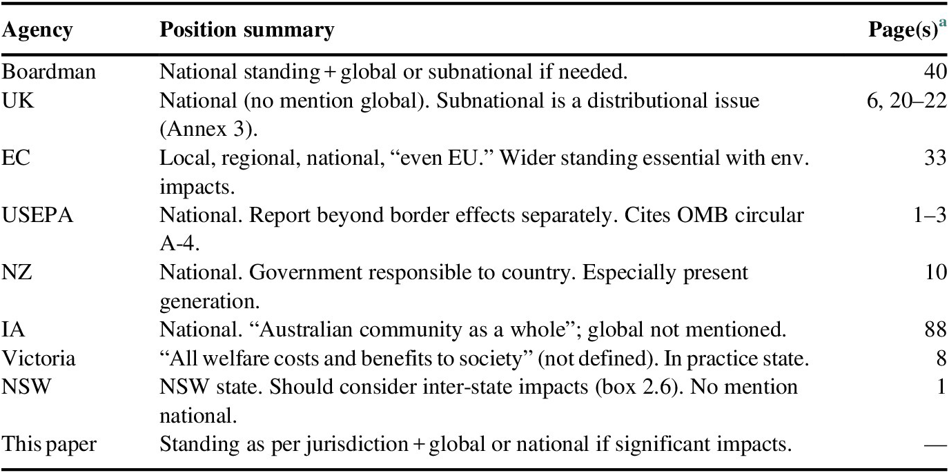
Table 1 summarizes the official positions on standing along with key page references in each guideline. Not surprisingly, the guidelines typically define standing in CBA studies from their own jurisdictional perspective. Thus, the UK, USEPA, NZ, and IA guidelines define standing from a national perspective. On the other hand, NSW explicitly recommends state standing (and notes cross border impacts) but does not mention national CBA. Drawing on author’s experience in Victoria, Victorian CBAs are also based on the state (e.g., Applied Economics, 2007).

Table 1 Positions on standing.

Abbreviations: EC, European Commission; IA, Infrastructure Australia; USEPA, U.S. Environmental Protection Agency.

^a In this and following tables, key pages are cited. The texts may include further references.

Moreover, there is little discussion in the guidelines of possible alternative standings. The UK, NZ, and IA guidelines make no mention of global effects and NSW and Victoria do not mention national impacts. The USEPA (pp. 1–3) does note that effects beyond U.S. borders should be reported separately. The European Commission (EC) is the major exception. It notes (p. 33) that the community of interest may “even” be the European Union (EU) and that: “All projects must incorporate a wider perspective when dealing with environmental issues related to CO₂ and other greenhouse gas emissions with effects on climate change which are intrinsically non-local.”

Thus, generally, the guidelines do not accord with Boardman views. The national guidelines ignore possible global impacts and the state guidelines ignore national outcomes.

Of course, issues of standing involve both value judgments and efficiency outcomes. The value judgment implicit in Boardman, with which this writer agrees, is that it is not acceptable for jurisdictions to conduct policies or projects that advantage them, but which significantly disadvantage other countries (or states). It is also not efficient to exclude external effects, especially in federations. For example, excluding central government grants to states (or provinces) implies that these grants have zero cost. This would encourage nationally inefficient projects. On the other hand, reductions in central government welfare payments to local residents due, for example, to successful state-financed employment training programs, would be treated as costs to the state, not as transfer payments. This could discourage efficient state projects. Thus, consistent with Boardman, this paper’s view is that the guidelines should require a global or national CBA when there are significant external impacts.

Moreover, none of the guidelines explain how to implement standing, implying that defining beneficiaries and losers from projects is a simple process. This is often far from the case. For example, economic surpluses of external (non-local) entities should be excluded from national and state-based CBAs.Footnote ² Likewise, other benefits accruing to non-local entities from say transport or environmental projects would be excluded. And, as Dobes (Reference Dobes2019) has shown, identifying cross-border effects in closely related geographical entities may be complicated.

These complex implications of standing are generally not spelled out in the official guidelines. Our conclusion is that the issue of standing and how to apply the principle needs fuller discussion in most of the guidelines.

3 Core valuation principles

Valuation principles are at the heart of CBA and there are many important issues. Here, we discuss two core issues: the nature of the underlying welfare assumptions and the related issues of how to value welfare changes for individuals, especially welfare losses. Another important issue raised by Weimer (Reference Weimer2017) is whether individuals may behave irrationally and, if so, how to value benefits or costs in these cases. We simply note here that this important issue receives little discussion in the official guidelines and is not discussed in this paper.

The common starting position in CBA is the existing social welfare status. Under this approach, benefits are valued at the maximum amounts that individuals are willing to pay (WTP) for them and welfare losses at the minimum amounts that individuals are WTA as compensation. In both cases, individuals are assumed to be as well off (or no worse off) with the change as without it. This is known as the “compensating variation” (CV) approach.

Alternatively, if a policy change is deemed to be the appropriate starting point, the benefits are the amounts that individuals would be WTA as compensation for not having the change and the costs are the amounts individuals are WTP for the change. In this case, the reference point is the individual’s level of welfare with the change. This is known as the “equivalent variation” (EV) approach.

These principles and the implications for valuation are summarized in Table 2.

Table 2 Summary of valuation principles and methods.

Abbreviations: WTA, willingness to accept; WTP, willingness to pay.

Source: Knetsch et al. (Reference Knetsch, Yohanes and Jichuan2012).

For example, suppose government is considering whether to provide high-level hospital services in a regional center. Under the CV approach, we would estimate whether the regional residents would be WTP for these additional services. If the collective WTP amount exceeded the cost, the services would be provided. Under the EV approach, we would estimate the WTA amounts that residents would accept instead of the services. The services would be provided if the total WTA amount exceeded the cost. Of course, the underlying premise here is that WTA values are likely to be higher than WTP values.

This issue is complicated further by actual measures of consumer benefits [consumer surplus (CS)] derived from observed (Marshallian) demand curves. Observed demand curves allow for real income changes as well as for price substitution effects. By contrast, (Hicksian) demand curves hold real income constant and allow only for substitution effects as required by the CV (or EV) approaches. Boardman et al. (Reference Boardman, Greenberg, Vining and Weimer2018, pp. 76–78) describes and illustrates these differences.

Of course, these distinctions do not matter if the alternative measures produce similar results. WTP and WTA valuations are equal if the marginal utility of income is constant. However, when there are significant changes in income and consequently in the marginal utility of income, WTP and WTA values (and CV and EV valuations) are likely to differ.

In chapter 3 on microeconomic foundations, Boardman et al. (Reference Boardman, Greenberg, Vining and Weimer2018, p. 75) concludes that “under most circumstances, estimates of changes in CS, as measured by demand curves, can be used in CBA as reasonable approximations of individuals’ WTP to obtain or to avoid the effects of policy changes.” In an annex to the chapter, discussing CV and EV as well as CS, the text concludes (p. 80) that the income effects of price changes are usually small “and can be safely ignored in CBA” and that Marshallian demand curves are reasonable approximation of WTP. However, they note in italics that this may cause a bias where income changes are significant as with large changes in housing or wage rates. They also note (p. 81) the differences between CV and EV, but do not draw practical conclusions.

On the other hand, Boardman notes (p. 442) that while economic theory suggests that WTP values are close to WTA values for market goods, stated choice surveys suggest otherwise, in some cases eliciting WTA values up to five times WTP values. However, they note that this may be due to the lack of a budget constraint in WTA responses to surveys as well as to loss aversion. They conclude (p. 446) that it may sometimes be appropriate to include WTA values but with “social budget constraints to increase the likelihood that respondents will provide an economic response.”

Table 3 above provides official guideline positions on the valuation principles. Standard CBA practice is to take the present situation (base case) as an appropriate starting point for policy evaluation. This embodies the CV principle. But these valuation principles receive little discussion in most guides. The Green Book (UK Treasury, 2018) does not discuss these issues. The NZ, Victorian, and NSW guidelines do not mention EV, but, by emphasizing that the base case is current policy, they imply the CV principle without using that conceptual language. NZ, Victoria, and NSW mention WTA values, but do not provide any detail about their application, effectively minimizing their use. The IA guide briefly mentions CV and EV approaches as well as possible use of WTA values, but without prescription.

Table 3 Positions on valuation principles.

Abbreviations: CV, compensating variation; EV, Equivalent variation; EC, European Commission; IA, Infrastructure Australia; USEPA, U.S. Environmental Protection Agency; WTA, willingness to accept; WTP, willingness to pay.

By contrast, the EC guide explicitly discusses the CV and EV principles and recommends CV and WTP values. It also notes that WTA values may be appropriate within the CV approach but does not provide guidance detail.

By even more contrast, the USEPA guide provides a thorough discussion of CV/EV choice. CV uses the welfare levels without environmental improvements; EV uses the levels with improvements. With CV, to enact policy, WTP for improvement must offset business cost of improvement. With EV, policy is enacted if WTA values for not having the improvement exceed the costs of improvement. As USEPA points out (p. 7–7), WTP is consistent with firms and individuals having the right to pollute. WTA is consistent with individuals having a right to a clean environment. It concludes (p. 5-1) nevertheless that: “The baseline of an economic analysis is a reference point that reflects the world without the proposed regulation.” And, while it notes that direct valuation studies are not possible for non-market goods, it acknowledges (pp. 1–12) that “most indirect valuation studies are based on Marshallian demand functions in practice, in the hope of keeping the associated error small.”

In effect, if not by explicit reasoning, the guidelines broadly follow the Boardman view that the starting valuation position is the CV view of the world and that benefits (CSs) can be valued using Marshallian demand curves or concepts to estimate WTP values. This is undoubtedly practical. However, the guidelines could be clearer about the value judgments underlying these valuation principles by reference, possibly in an annex, to CV and EV, and what these approaches imply on rights to health services, environmental goods, and so on. These are important value judgments and clarity could help to reduce misunderstandings on these issues between economists and other disciplines, notably environmental or social disciplines.

A more practical issue is the omission in the guidelines of any guidance on possible application of WTA values in terms of contexts and magnitudes. Certainly, for small changes in income (say up to $100) and most plausible forms of the utility function, differences between WTP and WTA amounts are likely to be minor and can be ignored. However, losses are often far higher than this, as for example, with household disruptions from major transport infrastructure projects. Citing Tunçel and Hammitt (Reference Tunçel and James2014), Boardman found that WTA values are often some five times higher than WTP values, especially for public and non-market goods. While recognizing the practical issues in estimating WTA values, in our view, this is an area for more consideration.

4 Project scope: additional economic benefits

The scope of CBA evaluations is a critical issue. The wider the scope of possible benefits, the higher the net benefit of a policy or project. Additional economic benefits, beyond user benefits in the primary market, include an array of possibilities. These include various impacts in related markets and second-round flow-on effects (multipliers). Disagreements on scope are at the heart of many disagreements about inputs and outputs in cost-benefit studies.

Moreover, discussion is often complicated by different uses of the term “secondary.” Secondary may refer to impacts in related (secondary) markets or to second-round flow-on impacts from first-round benefits (multiplier effects). Figure 1 provides a simple diagram, which distinguishes between first-round effects, including direct and indirect market impacts, and second-round flow-on income and employment multipliers from these first-round effects.

Figure 1 First and second round effects of projects and policies.

It follows that the main issues are (i) when to include first-round indirect benefits or costs of third parties or related markets and (ii) whether, if ever, to include second-round multiplier effects.Footnote ³ Related markets may include producer surpluses of suppliers of inputs to the project and/or losses incurred by suppliers of substitute goods and services. In both cases, the gains or losses respectively arise where prices depart from marginal costs of production. In some cases, notably related to transport infrastructure, related markets impacts are associated with “wider economic benefits,” especially productivity gains from agglomeration economies or place making benefits, rather than clearly identified complementary inputs or substitute goods (UK Department for Transport, 2018).

Boardman (chapter 7) describes how it is generally appropriate to include specific related market effects (described in this text as “secondary benefits”) when markets are non-competitive or distorted. This may also occur for infrastructure projects where prices do not reflect costs (p. 173). The text does not discuss the concept of wider economic benefits. On the other hand, the text does not support including second-round (multiplier) flow-on effects in CBA, except for distributional analysis. In discussing project scope (p. 9), the text warns: “It is often incorrect to include secondary, or ‘knock-on’ effects” meaning, it appears, multiplier effects. These reservations are strongly reinforced in pp. 173–175.

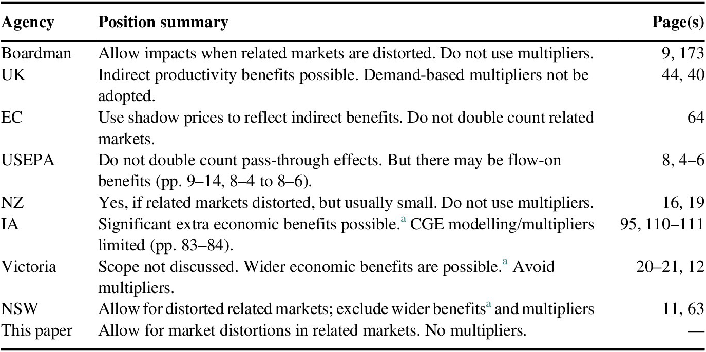
Table 4 provides a summary of official positions on economic scope. There is a wide agreement that CBAs should not include second-round multipliers. As expressed in the NZ guide (p. 55), “CBA typically assumes that the increased activity from the project crowds out other activity. The total amount of activity in the economy does not change.” However, the guide (p. 19) does note possible exception for multipliers when unemployment is significant. Also, while the USEPA guide states in chapter 8 that impacts that are passed on in changing prices are transfers in CBA (and so do not affect the CBA results), in chapter 9, it says that income gains may have an economic multiplier effect through increased expenditure.

Table 4 Positions on project scope: additional economic benefits.

Abbreviations: CGE, computable general equilibrium; EC, European Commission; IA, Infrastructure Australia; USEPA, U.S. Environmental Protection Agency.

^a Should be included only as sensitivity test, not as part of central CBA result.

The three guidelines that discuss effects in related distorted markets (NZ, NSW, and EC) follow the Boardman principles. The other guides do not provide specific guidelines for these markets.

Greater differences emerge in considering wider economic benefits (WEBs). These are discussed in the UK and Australian guidelines but not in the EU, USEPA, or NZ guidelines. The UK guide (p. 44 and elsewhere) opens the door to including significant productivity/agglomeration benefits related to infrastructure over and above-user benefits. This is reinforced in UK Treasury (2015), Valuing infrastructure spend: Supplementary guidance to the Green Book. The three Australian guidelines cited here also allow for possible WEBs. However, noting the uncertainties about them, they advise that where WEBs may exist, they should be included in sensitivity tests rather than in central results.

Thus, there is a fair degree of concordance between the Boardman positions on economic scope and the guidelines with high agreement on the non-use of multipliers.Footnote ⁴ There is also a fair measure of agreement on treatment of impacts in related markets. However, the treatment of these issues could usefully be addressed more explicitly in several guidelines. The main difference is on inclusion of WEBs which Boardman does not address, presumably implying unimportance, which the UK guideline supports as do the Australian guidelines more tentatively. In a separate paper, Abelson (Reference Abelson2019) concluded, for many reasons, that WEBs should be treated very cautiously. Chief among the reasons are that transport infrastructure may not have significant employment agglomeration impacts, that residential development may occur in any case, and that land value uplift should not be double counted with transport user benefits.

5 Changes in real values over time

All CBAs include forecast values in constant prices. However, real (relative) values may change over time. For example, a resource, or environmental asset, may be expected to become scarcer or more plentiful over the life of a project with relative values rising or falling accordingly over time.

Boardman (p. 220) has a clear view on this. “Relative prices may change. Analysts should always consider this possibility, especially for long-lived projects. Fortunately, there is no conceptual difficulty in handling relative price changes.”

Table 5 shows official positions on the treatment of real values over time. Only the NZ guide addresses the issue explicitly. The issue is discussed implicitly in the USEPA guide. It is not discussed in the EC or UK guide or in any Australian guide.

Table 5 Positions on real values over time.

Abbreviations: CBA, cost-benefit analysis; EC, European Commission; IA, Infrastructure Australia; STPR, social time preference rate; USEPA, U.S. Environmental Protection Agency.

The NZ guide accepts allowing for relative price changes in principle but recommends applying this with great caution because of difficulty in forecasting relative price changes. It notes (p. 18) that it may be possible to follow forward market signals (futures markets). The USEPA guide does not discuss the principle explicitly but notes the difficulty of forecasting technological changes and market responses.

Although the UK guide does not discuss changes in relative values, it recommends using a lower SDR for life and health values (see Table 7 below). Thus, implicitly it is advocating an increasing value of life over time. The NZ guide also recommends that the value of statistical life (NZ$3.85 million in 2013 prices) should be indexed to changes in average hourly earnings, presumably because WTP values would rise with income rather than with inflation, which would be changes in real terms. This writer has a problem with regarding future lives as more valuable than ours. This is also inconsistent with the equity approach that values life equally across all individuals (of standing) in standard CBA studies.Footnote ⁵ It may also be noted that the USEPA value of statistical life rises with inflation (pp. 7–8), which is constant in real terms.

To conclude, we agree with Boardman that the issue of real (relative) values over time should be explicitly considered. For example, arguably the value of business travel-time savings would rise with real earnings. But, as NZ and USEPA note, this is a complex forecasting matter. It is also important that, if changes in real values are adopted, they be adopted consistently and centrally and not by analysts on individual projects.

6 The marginal excess tax burden

The issue here is the marginal cost of public funds. Is this simply marginal expenditure or should it include an allowance for the METB associated with distortions of labor supply, savings, or consumption with various taxes? And, if METB is included, what value should be allowed?

Boardman (pp. 69–73) describes how funds raised by taxation have a METB and recommends that METB on net funds raised by taxation should be included in CBA. Drawing on several estimates of METB in the USA, the text estimates an average METB = 0.23 (23 cents in the dollar) for federal projects based on income tax financing. On the other hand, for local government projects financed by property tax, METB = 0.17.

Table 6 shows the positions of the official guides on allowance for the marginal excess tax burden. Four of the seven guides do not discuss the issue, which implies no allowance for METB. NSW recommends not adopting a METB in the central case, but possibly including in sensitivity tests. Victoria recommends a low METB = 0.08 reflecting land tax, but no allowance when tax revenue is fixed or for Commonwealth grants or when revenue is funded by efficient user charges. In practice, in the writer’s experience (extensive in NSW, limited in Victoria), METB is not applied in NSW or Victorian CBAs, including in sensitivity tests. This leaves NZ as an outlier recommending a METB = 0.20.

Table 6 Positions on marginal excess tax burden.

Abbreviations: EC, European Commission; IA, Infrastructure Australia; METB, marginal excess tax burden; USEPA, U.S. Environmental Protection Agency.

So, where should we go from here? Follow Boardman, ignore METB (as advised, e.g., Bos et al., Reference Bos, van der Pol and Gerbert2019) or search for a compromise? The leading technical literature (e.g., Johansson & Kristrom, Reference Johansson and Kristrom2016, pp. 39–41) tends to support the inclusion of METB. Thus, in comprehensive guides, it is appropriate to recognize that the METB is a real cost.

However, there are two substantive reasons for not including METB cost multipliers in CBA studies. First, taxes are generally fixed independently of specific projects. Thus, the cost of a project is the opportunity cost of the forgone project(s), not the marginal tax raised. As argued below, this should be recognized in the choice of SDR. Where tax is fixed, it would be inappropriate to add METB.Footnote ⁶ Second, as Boardman recognizes, revenues may partly or even wholly offset taxes with net outgoings less than gross tax. Accounting for this would be challenging. Including METB on a differential basis on a project by project basis would raise serious practical issues of consistency between projects.Footnote ⁷

7 The social discount rate

There are two main concepts of the SDR: the social opportunity cost of capital (SOC) and the social time preference rate (STPR). There are, in turn, two main versions of SOC: the return on investment (ROI) forgone in alternative projects (including market projects) or a weighted cost of funds (WCOF) reflecting the estimated proportions of investment and consumption forgone based on the sources of the project funding. ROI is forward looking. WCOF reflects how funds have been raised. The STPR values benefits and costs based on social values of consumption over time. This typically discounts future consumption as the marginal utility of consumption falls as incomes are expected to rise and may allow for pure time preference. The SOC based on ROI is typically around 6–7% per annum, while the STPR is usually around 2.5–3.5%. Hence, this is a very consequential issue.

One way to resolve this dilemma is by using a shadow price of capital (SPC). A SPC is estimated by discounting the forecast returns on investment forgone by the STPR. The STPR is then applied in turn to the forecast project net benefits based on the estimated SPC employed. Where the funds employed would otherwise have been fully invested, this gives similar outcomes (positive or negative) to the ROI approach.

Boardman concludes (p. 260) that there is general agreement that the SPC approach is the appropriate one, but that this is not practical for various reasons including whether projects are funded from investment or consumption forgone. In lieu of this approach, they recommend what they call the “optimal growth rate method” which, in their account, means application of the STPR. They also recommend use of declining SDR over time. Thus (p. 258), they recommend 3.5% SDR from year 0 to 50, and then declining rates over the next 50 and 100-year periods reaching 0% in year 300. They also recommend sensitivity testing with alternative discount rates.

Table 7 provides official positions on the SDR. There is a sharp geographical divide. The northern jurisdictions (UK, EU, and USEPA) follow Boardman in recommending a STPR. In the case of the USEPA, this reflects the impacts of environmental policy regulations, which the USEPA notes would affect consumption more than investment. The UK also recommends a declining rate in the long run. New Zealand and the Australian jurisdictions recommend a SOC discount rate. The NZ and NSW rates are based on the ROI approach. The Victorian SDR is apparently based on the WCOC approach (see Fernandez, Reference Fernandez2019).

Table 7 Positions on the social discount rate.

Abbreviations: EC, European Commission; IA, Infrastructure Australia; ROI, return on investment; SPC, shadow price of capital; STPR, social time preference rate; SOC, social opportunity cost; USEPA, U.S. Environmental Protection Agency.

On the other hand, differently from Boardman but still following the STPR principle, the northern jurisdictions recommend different STPRs for different situations. The UK recommends that as life becomes more valuable, life and health should be discounted at lower rates. We disagreed with this approach in Section 5 above. In contrast, the EC recommends higher STPR rates in countries where the expected rate of growth of incomes is higher. This is consistent with the standard Ramsey STPR formula where the STPR rises with higher forecast rates of economic growth and therefore less marginal value from future consumption.

Turning to the Australian and NZ guidelines, IA and NSW recommend that a central 7% SOC rate be applied (along with sensitivity tests for other rates). NZ and Victoria recommend central rates of 6 and 7%, respectively, but that they should vary with circumstances. The NZ approach allows the rate to vary with the value of β (the correlation with market risk) in the CAPM (capital asset pricing model) component of the standard WACC (weighted average cost of funds) model with the recommended rate falling or rising with lower or higher β. The Victorian approach allows a lower SOC of 4% for “core public services,” such as health and education where benefits are hard to monetize, in contrast with transport and housing where benefits are more quantifiable.

In conclusion, this paper agrees with Boardman on the principle of the SPC approach, but also that this approach is not practical for general use. Given this, as argued by Abelson and Dalton (Reference Abelson and Dalton2018), this paper supports a SOC discount rate based on the forward-looking ROI principle rather than on the backward looking WCOF. Selecting projects with lower (STPR) rates of return than the ROI is inefficient and does not optimize welfare growth. Given re-investment, selecting efficient projects with higher rates of return can benefit future generations as well as present ones. This paper is also cautious about adopting different SDRs for different projects based on assumptions about less or more covariance with market risks or with greater or less ease of monetizing benefits. These assumptions are hard to verify and implement, and could cause more distortions than they would resolve.

8 Benefit-cost ratios

Discussions of BCRs are complicated by the lack of a clear single definition. The common (standard) definition is:

(1)$$ \mathrm{BCR}=\mathrm{PV}(B)/\mathrm{PV}\left(I+C\right), $$

where PV is present value, B is benefits, I is capital investment, and C is all other costs. An alternative, less common, definition is:

(2)$$ \mathrm{BCR}=\mathrm{PV}\left(B\hbox{-} C\right)/\mathrm{PV}(I). $$

The Boardman text (pp. 34–35) does not formally identify the BCR but implies Equation (1) and does not discuss Equation (2). However, the text has a clear position on standard Equation (1). After noting that the BCR has been proposed as an alternative decision rule, the text states (p. 15): “This is one area where there is a right answer and wrong answers. The appropriate criterion to use is the NPV rule …The other rules (including the IRR (internal rate of return)) sometimes give incorrect answers; the NPV rule does not.” The text points out that (i) the NPV criterion is generally preferred way to rank projects because the BCR is biased toward small projects and (ii) the BCR may be manipulated by classifying some costs as negative benefits (classification issue). They conclude (p. 35): “We recommend that analysts avoid using BCRs to rank policies and rely instead on net benefits.”

Table 8 summarizes the official positions on BCRs. All these guides cite or imply the standard BCR as in Equation (1). Victoria is the only jurisdiction to cite Equation (2).

Table 8 Positions on the benefit-cost ratios.

Abbreviations: BCR, benefit-cost ratio; EC, European Commission; IA, Infrastructure Australia; NPV, net present value; PV, present value; USEPA, U.S. Environmental Protection Agency.

IA gives a further possible option as BCR = NPV/I. However, this is not a further option as

(3)$$ \mathrm{NPV}/I=\mathrm{PV}\left(B\hbox{-} C\hbox{-} I\right)/\mathrm{PV}(I)=\mathrm{PV}\left(B\hbox{--} C\right)/\mathrm{PV}(I)\hbox{--} 1, $$

that is, this equals BCR in Equation (2) – 1. This is redundant when Equation (2) is employed.

As shown in Table 8, the official guides take various approaches. Several guides (EC, USEPA, NZ, and Victoria) cite bias and/or classification problems associated with the standard Equation (1). But they reach different conclusions. EC suggests that Equation (1) is satisfactory when there are budget constraints. USEPA excludes the BCR from its proposed reporting template. NZ says Equation (1) provides useful intuitive understanding of outcomes, despite ranking problems. Only Victoria recommends the use of Equation (2) with capital constraints. On the other hand, the UK and NSW guides support use of BCR in Equation (1) without qualifications.

Given the clear Boardman views and the contrasting muddled set of official recommendations, where does this reviewer stand? Well, first, we agree fully with Boardman’s criticisms of Equation (1) as biased toward small projects and subject to manipulation due to treatment of costs as negative benefits in the numerator or as costs in denominator.Footnote ⁸

However, the BCR as per Equation (2) is relevant to decision making under capital constraints when the returns on an agency’s marginal projects exceed the marginal return elsewhere. In this case, the agency should select projects in order of their present value per unit of constrained capital until the capital is exhausted. Box 1 illustrates how the BCR ranks smaller projects more favorably than the NPV criterion, but also how Equation (2) maximizes NPV under a budget constraint (here a simple first year constraint).

Box 1 NPV versus BCR criterion

Thus, Equation (2) is appropriate when ranking projects subject to capital constraint. Arguably, the constraint could include ongoing recurrent, as well as capital, government expenditure. In this case, government recurrent expenditures would also be below the line and other costs above.

9 Treatment of risk and uncertainty

There are numerous issues regarding the treatment of risk and uncertainty. Here, we discuss two of these issues. One is how to represent the distributions (the variances) of the costs and benefits in a CBA? The second is whether to allow for option values? An option value is the difference between the expected use value and the total WTP for an asset or service. Thus,

(4)$$ \mathrm{WTP}=\mathrm{EUV}+\mathrm{OV}=\mathrm{OP}, $$

where EUV is expected use value, OV is option value, and OP is known as the option price.Footnote ⁹ Note, importantly that, as shown by Freeman (Reference Freeman1984), while option value is generally positive when individuals are risk averse, it can be negative when individuals are uncertain about future income.

The discussion of option values is sometimes complicated by two other option concepts: “quasi-option values” and “real options.” Quasi-option value is the value of information that can be gained by more time or study (Pearce et al., Reference Pearce, Giles and Mouranto2006). The value is the benefit from deferring and improving a project decision. This needs to be weighed against the costs of deferment. A real option arises through variations in the time or mode of project delivery, such as staging the various components of a project. Morton-Cox (Reference Morton-Cox2018) provides a helpful discussion of real options.

Boardman devotes two chapters to the two topics that we have identified. Chapter 11 discusses expected values (EVs). Chapter 12 discusses option values. Chapter 11 concludes (p. 298) that the expected value analysis is the appropriate way to deal with an uncertain range of costs or benefits. Implicitly, this is a risk neutral approach.

The text notes conceptual support for the use of option prices at several points. “Economists now generally consider option price … to be the theoretically correct measure of willingness to pay in circumstances of uncertainty or risk.” (p. 315). “The conceptually correct way to value a policy involving risks is to sum the ex-ante amounts that individuals … would be willing to pay for it.” (p. 316). “Option price is the conceptually correct measure of benefits.” (p. 324).

However, Boardman also states: “In practice analysts usually do not convert net benefits to certainty equivalents or option prices. Specifically, they use expected values rather than option prices because the former can be estimated from observable behavior, whereas the latter requires contingent valuation surveys.” (p. 263, endnote 6). The text observes (p. 315) that economists typically estimate the benefits using EV estimates. “Unfortunately, confidently signing, let alone quantifying option price is often not possible.” (p. 332).

Table 9 provides official positions on the use of expected values and option values (or prices). As a generalization, most of the guidelines discuss treatment of risk and uncertainty at some length with various discussions of the nature of risks, contingencies, appraisal optimism (especially in UK guide), sensitivity tests, the use of real option analysis, and identifying and managing of risk. However, there is limited discussion of the use of expected values and virtually none on option values.

Table 9 Positions on uncertainty and risk.^a

Abbreviations: EC, European Commission; ENPV, expected net present value; EV in this table and section = expected value; IA, Infrastructure Australia; PV, present value; USEPA, U.S. Environmental Protection Agency.

^a Focus in this table: expected values and option values, not sensitivity tests and risk management.

^b P50 is median not mean value.

The only guides to explicitly discuss and recommend use of EVs are the EC and NSW guides. The IA guide recommends EV for costs but allows use of P50 if a forecast cost distribution is not available (which is a questionable assumption with typical skewed cost distributions). It does not discuss how to deal with distributions across benefits. The NZ guide implicitly (but very briefly) recommends EVs. The Victorian guide describes Monte Carlo analysis without mentioning EVs. The other two guides do not mention EVs. The EC is the only guide to mention option values but does not discuss them in any detail.

Turning to our concluding thoughts, first, we agree with Boardman that CBA should generally be based on expected values (and expected net present values, ENPVs). This risk-neutral approach is efficient and appropriate for most public policies and project decisions. Occasionally, when projects have a large impact on a community, government may choose a safer project with a lower ENPV. Following Boardman, this should be an explicit approach in CBA guides along with guides on how to treat issues like contingency costs. In some cases, contingencies are allowances for project features that cannot be fully designed or forecast in advance but can be expected and are part of a median forecast. In other cases, contingencies drive P90 forecasts.Footnote ¹⁰

Option values are more complex. In effect, option values are included in WTP (option) prices obtained from stated preference surveys. They are not included in values obtained from market prices or other revealed preference valuation methods. The usual implicit assumption is that where these differences exist, they are likely to be small and can be ignored. This paper cannot provide any better approach.