


1. Introduction
In this paper we are concerned with the stochastic modelling and analysis of the self-similar patterns observed in a class of elastic crystals undergoing a shape change at the level of the atomic lattice as a consequence of a first-order thermodynamic phase transformation. This is the austenite-to-martensite (AM) phase transformation, a solid-to-solid transition observed in steel and shape-memory alloys driven by temperature or an applied mechanical stress [Reference Bhattacharya5]. In a temperature-driven transformation, the material evolves from austenite, the highly symmetric and highly homogeneous crystal phase (typically the cubic lattice), as temperature decreases via a series of ‘avalanches’ from one energetically metastable state to another. The energy releases associated with the avalanches are manifested in the nucleation and growth of thin regions where the molecules are arranged locally according to a lower-symmetry lattice (martensite) as well as in acoustic waves generated by their moving interfaces. As a result, an intricate highly inhomogeneous pattern soon emerges, populated by sharp interfaces that separate thin plates composed of mixtures of different martensitic phases (i.e. rotated copies of the low-symmetry lattice) and planes separating the austenite from martensite – what in the materials science literature is known as a microstructure (see Figure 1 and also the movie https://www.youtube.com/watch?v=Bwy8xC3hous supplementary to [Reference Song, Chen, Dabade, Shield and James30]). An important point is that the austenite-to-martensite transformation is purely structural. It does not involve chemical reactions or diffusion but only a morphological change in the atomic arrangements. The nucleation sites of the interfaces are influenced by the state of disorder of the system, lattice defects and impurities, and typically require a probabilistic modelling approach. However, their orientation and directions of propagation are determined by the kinematic compatibility of the various crystal phases, which are defined by rigid algebraic relations incorporated in the symmetry properties of the transformed lattice.
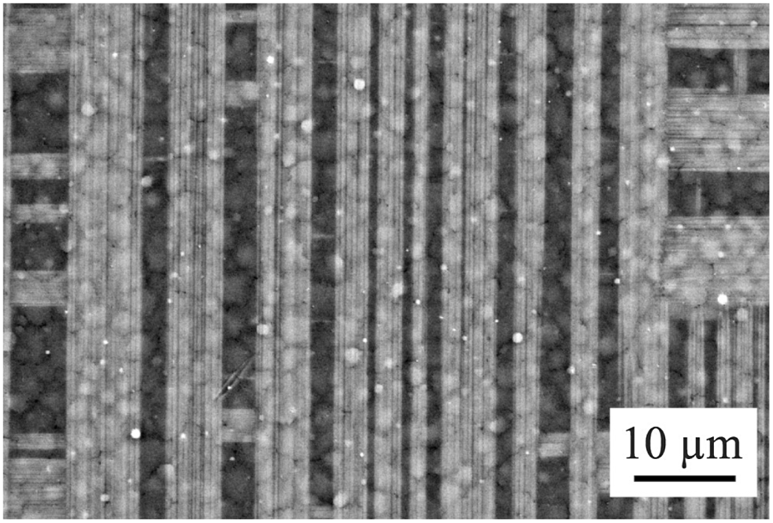
Figure 1. Snapshot from a temperature series of scanning electron micrographs of the alloy NiMnGa. Here the dark grey area corresponds to untransformed material (austenite), and the light grey ‘needles’ evolving in the vertical or horizontal direction correspond to the domain already transformed into a martensitic phase. Courtesy of Robert Niemann and reproduced with the permission of the author.
Statistical analysis of the acoustic activity captured during the transformation [Reference Salje, Koppensteiner, Reinecker, Schranz and Planes29] shows that several macroscopic variables such as amplitude, duration, and energy of the acoustic waves exhibit a power law behaviour and a characteristic exponent. More experimental evidence [Reference Planes, Mañosa and Vives28] seems to suggest that the exponents measured are indeed characteristic of an entire class of materials undergoing a specific AM transformation, leading to the conclusion, which constitutes the ansatz of this work, that materials with different chemical composition may be grouped into universality classes identified uniquely by the symmetry reduction of the AM transformation.
Although of great relevance for technological applications and despite the substantial literature on the analysis and prediction of the statics of this transformation, it is remarkable that the dynamics of the martensitic transition is still to date an outstanding open modelling problem [Reference Ball1, Reference Müller24].
The modelling approach we propose for the dynamics of the AM transformation consists of a fragmentation process in which the microstructure evolves via the formation of thin plates of martensite embedded in a medium representing the austenite. Here the plates are idealized as planar surfaces which nucleate and propagate according to a stochastic process in space and time and are allowed to grow parallel to a given set of admissible directions. Our main focus will be on a simple model in two dimensions, and we imagine that the unit square represents the reference configuration occupied by the material in the austenitic phase. In our caricature model, nucleation events occur as a Poisson process in this domain, and as each point appears it generates, with equal probability, a plate which propagates orthogonally in either the x or y direction. These plates propagate until they hit part of the structure of plates that has already appeared or the boundary of the domain, and as a result a complicated structure of rectangles soon emerges. A physical process which generates patterns of the type we are interested in is shown in Figure 1, and the initial steps of a realization of the model are shown in Figure 2.
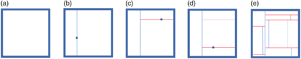
Figure 2. (a)–(d) The initial stages of a fragmentation process. (e) The configuration after 11 nucleation events.
It is believed that the acoustic emissions in experiments on the AM transformation are associated with the formation of plates, and the power laws observed should correspond to power laws in the number of plates. By encoding our probabilistic model into a general branching random walk, we are able to obtain predictions for the asymptotic behaviour of features of the random pattern generated. The question that we address is the behaviour of the number of plates of a given size. We treat two versions of this problem.
-
(i) For a complete fragmentation we consider the number of interfaces above a certain size and obtain a power law for this quantity.
-
(ii) We look at the asymptotics for the sizes of small interfaces and show that this depends on the way the pattern is generated and is not a power law.
An approach based on a fragmentation process for describing martensitic microstructure was adopted for the first time in [Reference Pasko, Likhachev, Koval and Kolomytsev27], to the best of our knowledge. Rather than focusing on the mathematical analysis of fragmentation models, [Reference Pasko, Likhachev, Koval and Kolomytsev27] performs data analysis on the structural properties of a two-dimensional pattern obtained from a fragmentation process via Fourier transforms. We also refer to [Reference Torrens, Illa, Vives and Planes31] for an alternative probabilistic model based on a fragmentation scheme which takes place over a sequence of finite lattices and addresses our first question. Besides the discrete nature of the model in [Reference Torrens, Illa, Vives and Planes31], the main difference from the present investigation lies in the mathematical approaches adopted for the analysis. In [Reference Torrens, Illa, Vives and Planes31] the investigation is focused on the exact solution of a complicated finite-difference equation for the conditional probability of splitting events occurring at the lattice level, and the outcome is limited to the construction of the asymptotic mean profile of the geometric quantities of interest. Conversely, in the present scenario, general branching process theory provides finer information on the shape of the asymptotic distribution of the interfaces, as it shows that there is almost sure convergence of the quantities of interest to a limit random variable as well as estimates on the tail of this random variable. It also allows us to vary the model more easily.
There are many papers that discuss models for patterns created by random fragmentation. This particular fragmentation model is referred to as the Gilbert tessellation in [Reference Mackisack and Miles23], where some features of the patterns are discussed. For mathematical work on the analysis of other fragmentation processes of relevance here, see [Reference Bertoin4] and [Reference Harris, Knobloch and Kyprianou19]. In the scalar case, we refer to [Reference Derrida and Flyvbjerg14] and [Reference Frontera, Goicoechea, Ràfols and Vives15], where a simple fragmentation model was introduced for the description of first-order phase transitions occurring as avalanches. For two-dimensional fragmentation processes there is work on quadtrees, which provides a more sophisticated analysis [Reference Broutin, Neininger and Sulzbach11] of a model related to the one we discuss here, as well as the recent work [Reference Callegaro and Roberts12], which gives an analysis of a model allowing the fragmentation to depend on the shape of the rectangle. Alternative approaches may be found in work on random tessellations. For tessellations of a compact region generated by iterations we refer to [Reference Nagel and Weiss25], and branching wise [Reference Georgii, Schreiber and Thäle17].
1.1. The model
The model divides the unit square up into a succession of rectangles which each get broken up into smaller and smaller pieces. The initial reference configuration is a unit square (Figure 2(a)) representing a homogeneous lattice in the high-symmetry phase (austenite). A point is selected in the square according to a uniform probability distribution, and a line through the point is drawn in one direction, either horizontal (with probability p) or vertical (with probability
 $1-p$
). The line extends through the square until it hits the boundary of the domain, and as a result the initial square is fragmented into two rectangles (Figure 2(b)). Now we iterate the procedure by picking a second point, again chosen according to a uniform probability distribution in the initial unit square, and draw a line passing through this point in either direction, horizontal or vertical with probability p and
$1-p$
). The line extends through the square until it hits the boundary of the domain, and as a result the initial square is fragmented into two rectangles (Figure 2(b)). Now we iterate the procedure by picking a second point, again chosen according to a uniform probability distribution in the initial unit square, and draw a line passing through this point in either direction, horizontal or vertical with probability p and
 $1-p$
respectively (in Figure 2(c), the horizontal direction). Now the line extends through the domain until it hits the boundary of the unit square or a part of the domain which has already transformed.
$1-p$
respectively (in Figure 2(c), the horizontal direction). Now the line extends through the domain until it hits the boundary of the unit square or a part of the domain which has already transformed.
We continue iterating this procedure by choosing a nucleation point at random in the unit square and splitting the rectangle containing it, soon resulting in a complicated pattern (Figures 2(d) and 2(e)). The requirement that interfaces cannot overlap is an important ingredient of the model inspired by experiments. It constitutes the modelling mechanism for a material where the parts that have already transformed into martensite cannot evolve any further.
The procedure described above is equivalent to requiring the nucleation to occur in a rectangle with a probability proportional to its area. This process can be continued indefinitely to get a complete fragmentation of the unit square. It is easy to see that, as each rectangle is split in two and the future evolution inside a rectangle is independent of what occurs outside, the individual rectangles that arise can be encoded by an infinite binary tree, and then any pattern we see at a finite scale can be obtained by taking a cut through the branches of this tree. As this fragmentation model does not appear to lead to a tractable analysis, in Section 4 we will consider two different time parametrizations that lead to an exact asymptotic analysis.
Simulations of the outcome from three different versions are shown in Figure 3. For our discussion of power laws in Section 3 we consider a complete fragmentation, and hence the time parametrization of the evolution of the fragmentation is not important.
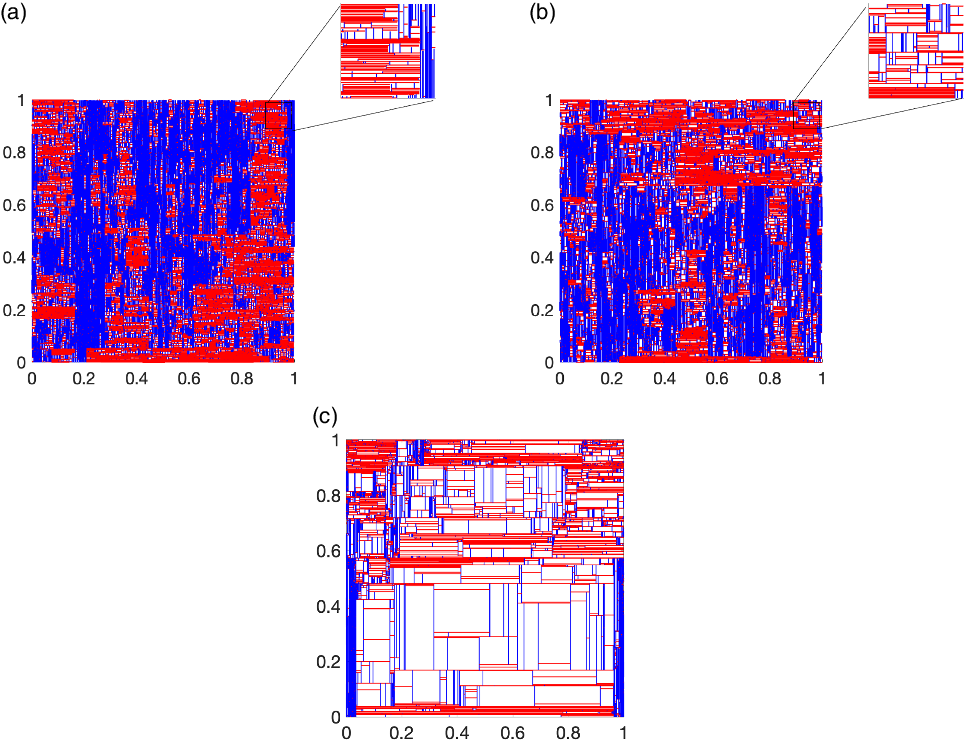
Figure 3. Microstructure obtained for the fragmentation model where at the time of each split we choose to split the rectangle of largest area (a) or a rectangle picked at random according to area (b). The pattern in (c) is obtained when each existing rectangle is split at the same time. All microstructures are composed of
 $2^{14}$
rectangles and
$2^{14}$
rectangles and
 $p={{1}/{2}}$
.
$p={{1}/{2}}$
.
In Figure 3(a) we show a realization of the pattern obtained when, at each iteration, a new nucleation point is selected according to a uniform probability distribution in the rectangle of largest area. In order to do this, we introduce a time parametrization so that at time t in this evolution all rectangles in the pattern have area at most
 ${\textrm{e}}^{-t}$
. This is the fragmentation mechanism analysed in Section 4.1.
${\textrm{e}}^{-t}$
. This is the fragmentation mechanism analysed in Section 4.1.
In Figure 3(b) we display a microstructure obtained for the fragmentation model where at each step a rectangle to be split is picked with probability proportional to its area. At a superficial level, structures in Figure 3(a, b) appear similar (see the insets), motivating our analysis of Figure 3(a).
Figure 3(c) shows a realization of the fragmentation process related to the one described in Section 4.2, which consists of splitting, at a fixed time, all the rectangles available regardless of their size. This fragmentation mechanism leaves
 $2^n$
rectangles after n steps, resulting in a pattern which, after a finite number of steps, is highly inhomogeneous. This is evident by observing the microstructures of Figure 3(a, b) which are composed of the same number of rectangles as Figure 3(c). The differences are made clear in the theoretical analysis in Section 4.
$2^n$
rectangles after n steps, resulting in a pattern which, after a finite number of steps, is highly inhomogeneous. This is evident by observing the microstructures of Figure 3(a, b) which are composed of the same number of rectangles as Figure 3(c). The differences are made clear in the theoretical analysis in Section 4.
In order to describe the model mathematically, we consider each rectangle as determined by two coordinates (a, b), which are the side lengths for the edges parallel to the horizontal and vertical axes respectively. Nucleation events occur as a Poisson process in time and lead to the formation of an interface. The nucleation point is uniformly distributed in the rectangle, and with probability p where
 $0\leq p\leq 1$
, the interface grows horizontally or with probability
$0\leq p\leq 1$
, the interface grows horizontally or with probability
 $1-p$
it grows vertically until it reaches the edges of the rectangle in the vertical or horizontal direction respectively. In this way we can see that the rectangle (a, b) evolves as
$1-p$
it grows vertically until it reaches the edges of the rectangle in the vertical or horizontal direction respectively. In this way we can see that the rectangle (a, b) evolves as
 \begin{equation*} (a,b) \to\begin{cases} \{(a,bU), (a,b(1-U)) \} & \text{probability $p$,} \\ \{(aU,b), (a(1-U),b) \}& \text{probability $ 1-p$,} \end{cases} \end{equation*}
where U is a uniform random variable on [0, 1].
The three-dimensional version of the fragmentation scheme is obtained analogously to the two-dimensional version by breaking down a unit cube into many rectangular cuboids by drawing planar plates. The procedure starts when a point is picked according to a uniform probability distribution on the unit cube. A plate through the point and orthogonal to either the
 $e_1$
,
$e_1$
,
 $e_2$
, or
$e_2$
, or
 $e_3$
direction (assuming the standard Euclidean basis), with probability respectively
$e_3$
direction (assuming the standard Euclidean basis), with probability respectively
 $p_1$
,
$p_1$
,
 $p_2$
, or
$p_2$
, or
 $1-p_1-p_2$
(with
$1-p_1-p_2$
(with
 $0\leq p_1,p_2,p_1+p_2\leq 1$
), splits the cube into two rectangular cuboids. We iterate this procedure by picking another point in the interior of the rectangular cuboid of largest volume and repeating the fragmentation procedure by allowing the plates to grow till they hit the boundary of the cube or another part of the domain which has already transformed (see Figure 4).
$0\leq p_1,p_2,p_1+p_2\leq 1$
), splits the cube into two rectangular cuboids. We iterate this procedure by picking another point in the interior of the rectangular cuboid of largest volume and repeating the fragmentation procedure by allowing the plates to grow till they hit the boundary of the cube or another part of the domain which has already transformed (see Figure 4).
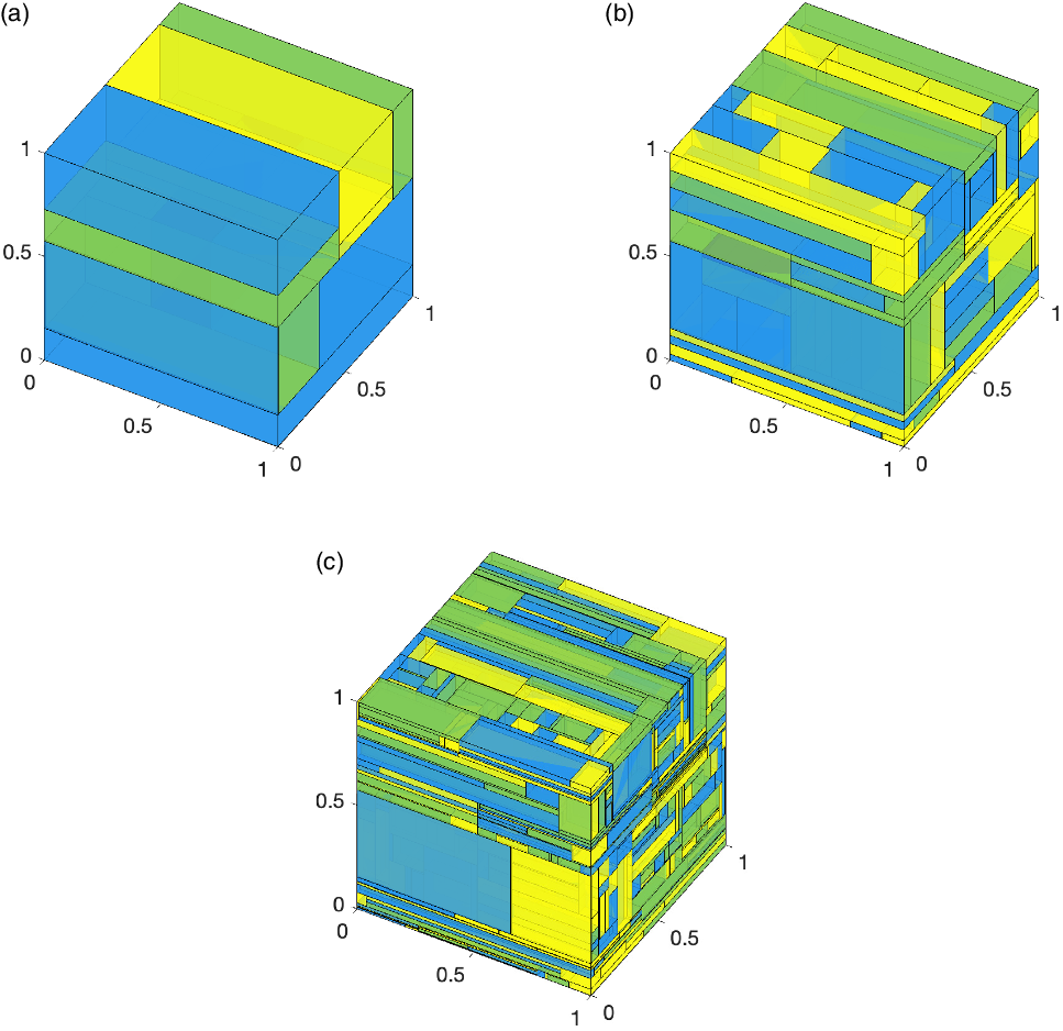
Figure 4. Three stages of the three-dimensional fragmentation model observed after n iterations: (a)
 $n=10$
, (b)
$n=10$
, (b)
 $n=100$
, (c)
$n=100$
, (c)
 $n=1000$
. Here
$n=1000$
. Here
 $p_1=p_2={{1}/{3}} $
.
$p_1=p_2={{1}/{3}} $
.
1.2. The main results
Our aim is to look at certain asymptotic quantities associated with the resulting collection of rectangles. In particular, we would like to determine the power law growth of the number of interfaces of at least a certain size. We now give two theorems that show two different types of asymptotic analysis that can be performed.
For our first result we do not consider a time parametrized evolution but look at the number of interfaces that have ever appeared with length greater than x. We will capture this quantity using a general branching process. In the two-dimensional version of the model this quantity is only finite if there is a bias in the direction of interface formation. However, in the three-dimensional unbiased version of the model, where
 $p_1=p_2=1/3$
, we obtain a power law exponent. More precisely, if we set
$p_1=p_2=1/3$
, we obtain a power law exponent. More precisely, if we set
 $N_h(x)$
to be the number of horizontal plates with area at least x in the limit pattern, then we obtain the following.
$N_h(x)$
to be the number of horizontal plates with area at least x in the limit pattern, then we obtain the following.
Theorem 1.1. There exists a non-degenerate random variable
 $W>0$
such that
$W>0$
such that
 \begin{equation*} \lim_{x\to 0} N_h(x)x^3 = W, \quad a.s. \end{equation*}
By symmetry the same result holds for the plates which are parallel to the other axial directions, and hence the total number of plates of more than a given area is power law with exponent 3. As this is a limit result, the initial domain is not important, and we would expect to see that any material occupying a region with smooth boundary that fragmented uniformly at random by plates orthogonal to the axial directions would have the exponent 3 for decay of the areas of the interfaces. We also obtain some left and right tail estimates on the limit random variable which capture its exponential decay at 0 and infinity. These are novel results, as this problem does not fit within the usual framework for tail estimates for the general branching process limit random variable.
Secondly we consider the asymptotics of the sizes of small rectangles in the pattern when we split the largest area first. As for the interfaces, analysis of rectangles is motivated and inspired by peculiar observations of low-hysteresis martensitic microstructures. The images in [Reference James20] (see e.g. page 22) show examples of complex ‘mosaic-like’ patterns composed of small polygonal domains characterized by sharp angles and edges. We analyse a simplified model with rectangles for the domains and the fragmentation model of breaking the largest rectangle first. Although physically less natural, Figure 3 shows that the appearance is reasonably similar to the original problem and this version of the model is tractable.
Let
 $\tilde{N}_t(A)$
denote the number of rectangles with side length
$\tilde{N}_t(A)$
denote the number of rectangles with side length
 $(a,b)\in A\subset [0, 1]^2$
at time t. Using a representation in terms of a general branching random walk, we will show the following in the unbiased case where
$(a,b)\in A\subset [0, 1]^2$
at time t. Using a representation in terms of a general branching random walk, we will show the following in the unbiased case where
 $p=1/2$
.
$p=1/2$
.
Theorem 1.2. Let S be a closed convex set with non-empty interior in
 $[0, 1]^2$
.
$[0, 1]^2$
.
-
(i) If
 $S\cap\{(a,b)\,:\, ab={\textrm{e}}^{-1}\}=\emptyset$
, then
\begin{equation*} t^{-1} \log{\tilde{N}_t({\textrm{e}}^{-t}S)} \to -\infty, \quad as\ t\to\infty,\quad a.s. \end{equation*}
$S\cap\{(a,b)\,:\, ab={\textrm{e}}^{-1}\}=\emptyset$
, then
\begin{equation*} t^{-1} \log{\tilde{N}_t({\textrm{e}}^{-t}S)} \to -\infty, \quad as\ t\to\infty,\quad a.s. \end{equation*}
-
(ii) If
$S \cap\{ (a,b)\,:\, ab={\textrm{e}}^{-1}\}\neq \emptyset$
, then setting
$\beta = \sup\{\gamma^*(a,b)\,:\, (a,b)\in S\}$
, where and
\begin{equation*} \gamma^*(a,b) = 2\sqrt{\log{a}\log{b}}, \quad ab={\textrm{e}}^{-1}, \end{equation*}
$\gamma^*(a,b)=-\infty$
for all other values of a, b, we have
\begin{equation*} t^{-1}\log{\tilde{N}}_t({\textrm{e}}^{-t}S) \to \beta, \quad as \ t\to\infty, \quad a.s. \end{equation*}


In the case where each rectangle splits independently at the same constant rate independent of size, the same limit theorem holds, but for a different function
 $\gamma^*$
which is strictly positive over an open set and given in (4.2).
$\gamma^*$
which is strictly positive over an open set and given in (4.2).
The structure of the paper is as follows. We describe the general branching process and general branching random walk in Section 2. In Section 3 we use a suitable general branching process to calculate the asymptotics for the number of edges greater than a given length in a biased version of the model. We establish an almost sure limit theorem with a non-degenerate limit random variable and obtain tail estimates for this quantity. In Section 4 we show how our model can be encoded as a general branching random walk. Using this we perform an analysis of the asymptotics for the number of rectangles of a given size within the pattern as a proxy for the lengths of the interfacial plates. In the case where we split the largest area first, this requires an extension of previous results on the general branching random walk.
2. General branching processes
In the next sections we will code up our fragmentation problems using a general branching process and a general branching random walk. The whole structure can be captured in a labelled tree as the evolution inside any rectangle does not affect what happens outside that rectangle. Thus in our tree each vertex will represent a rectangle, and we put labels on the vertices to capture the information that we need about the size of the rectangle. The natural setting for this is the theory of general branching processes.
In the Crump–Mode–Jagers or general branching process (GBP), we model the evolution of a population of individuals who evolve independently. In our version the typical individual x is born at time
 $\sigma_x$
, has offspring whose birth times are determined by a point process
$\sigma_x$
, has offspring whose birth times are determined by a point process
 $\xi_x$
on
$\xi_x$
on
 $[0, \infty)$
, and has a (possibly random) càdlàg function
$[0, \infty)$
, and has a (possibly random) càdlàg function
 $\phi_x$
on
$\phi_x$
on
 ${\mathbb R}$
called a characteristic. This can be extended to a general branching random walk (GBRW) if we include a process for the birth position
${\mathbb R}$
called a characteristic. This can be extended to a general branching random walk (GBRW) if we include a process for the birth position
 $\eta_x$
as well as the birth time. We will develop the set-up for the GBRW and then, by ignoring the spatial structure, we will have a GBP. We could just write the GBRW using a space–time point process but keep the separate form for the two components, as we use the two components in different ways.
$\eta_x$
as well as the birth time. We will develop the set-up for the GBRW and then, by ignoring the spatial structure, we will have a GBP. We could just write the GBRW using a space–time point process but keep the separate form for the two components, as we use the two components in different ways.
We now establish the model formally. Let
 $I_n = \cup_{k=0}^n {\mathbb N}^k$
and
$I_n = \cup_{k=0}^n {\mathbb N}^k$
and
 $I = \cup_k I_k$
. A sequence in I will be denoted
$I = \cup_k I_k$
. A sequence in I will be denoted
 $\textbf{i} \in I$
, though we will write
$\textbf{i} \in I$
, though we will write
 $i\in I_1$
.
$i\in I_1$
.
 $I_0$
is the empty sequence
$I_0$
is the empty sequence
 $\emptyset$
. We write
$\emptyset$
. We write
 $\textbf{i}\textbf{j}$
for the concatenation of sequences
$\textbf{i}\textbf{j}$
for the concatenation of sequences
 $\textbf{i}$
and
$\textbf{i}$
and
 $\textbf{j} \in I$
. For a point
$\textbf{j} \in I$
. For a point
 $\textbf{i} \in I\backslash I_n$
, let
$\textbf{i} \in I\backslash I_n$
, let
 $\textbf{i}|_n$
denote the sequence truncated to length n and let
$\textbf{i}|_n$
denote the sequence truncated to length n and let
 $\textbf{i}[n]$
be the nth element of
$\textbf{i}[n]$
be the nth element of
 $\textbf{i}$
. We write
$\textbf{i}$
. We write
 $\textbf{j} \leq \textbf{i}$
if
$\textbf{j} \leq \textbf{i}$
if
 $\textbf{i} = \textbf{j} \textbf{k}$
for some
$\textbf{i} = \textbf{j} \textbf{k}$
for some
 $\textbf{k}$
, and let
$\textbf{k}$
, and let
 $|\textbf{i}|$
denote the length of the sequence
$|\textbf{i}|$
denote the length of the sequence
 $\textbf{i}$
.
$\textbf{i}$
.
If
 $\textbf{i}$
has j children, then these are
$\textbf{i}$
has j children, then these are
 $\textbf{i} 1, \textbf{i} 2, \ldots, \textbf{i} j$
. A tree T is a subset of the space I such that:
$\textbf{i} 1, \textbf{i} 2, \ldots, \textbf{i} j$
. A tree T is a subset of the space I such that:
-
(i)
$\emptyset \in T$
the root of the tree; -
(ii)
$\textbf{i} \in T$
implies
$\textbf{i}|_k \in T$
for all
$k < |\textbf{i}|$
; -
(iii) if
$\textbf{i} j \in T$
for some
$j \in {\mathbb N}$
, then
$\textbf{i} 1, \textbf{i} 2, \ldots, \textbf{i} (j-1) \in T$
.


We have a one-to-one correspondence between trees and feasible realizations of the set of individuals in a branching process. In this paper, unless otherwise stated, from the next section the tree will be fixed as a binary tree.
We now introduce suitable labels on the tree. For each element
 $\textbf{i} \in T$
, let the life-story for
$\textbf{i} \in T$
, let the life-story for
 $\textbf{i}$
be
$\textbf{i}$
be
 $V_\textbf{i} = ((\xi_\textbf{i}, \eta_\textbf{i}), \chi_\textbf{i})$
. The
$V_\textbf{i} = ((\xi_\textbf{i}, \eta_\textbf{i}), \chi_\textbf{i})$
. The
 $V_\textbf{i}$
are independent and identically distributed (i.i.d.); the pair
$V_\textbf{i}$
are independent and identically distributed (i.i.d.); the pair
 $(\xi_\textbf{i}, \eta_{\textbf{i}})$
contains the birth times and locations of each offspring, where
$(\xi_\textbf{i}, \eta_{\textbf{i}})$
contains the birth times and locations of each offspring, where
 $\xi_{\textbf{i}} \,:\, {\mathbb R}_+ \to {\mathbb Z}_+$
(non-decreasing) is the birth time process,
$\xi_{\textbf{i}} \,:\, {\mathbb R}_+ \to {\mathbb Z}_+$
(non-decreasing) is the birth time process,
 $\eta_\textbf{i} \,:\, {\mathbb R}_+ \to {\mathbb R}^d$
is the birth position process, and
$\eta_\textbf{i} \,:\, {\mathbb R}_+ \to {\mathbb R}^d$
is the birth position process, and
 $\chi_\textbf{i} \,:\, {\mathbb R}_+ \to {\mathbb R}_+$
is the characteristic, a function used to count attributes of the individual. Then
$\chi_\textbf{i} \,:\, {\mathbb R}_+ \to {\mathbb R}_+$
is the characteristic, a function used to count attributes of the individual. Then
 $\xi_\textbf{i}(t)$
is the number of children born to
$\xi_\textbf{i}(t)$
is the number of children born to
 $\textbf{i}$
up to and including time t, and
$\textbf{i}$
up to and including time t, and
 $\xi_\textbf{i}(\infty)$
is the total number of children born to
$\xi_\textbf{i}(\infty)$
is the total number of children born to
 $\textbf{i}$
. For a general branching random walk, we make no assumption about the joint distribution of
$\textbf{i}$
. For a general branching random walk, we make no assumption about the joint distribution of
 $(\xi_\textbf{i}, \eta_\textbf{i})$
and
$(\xi_\textbf{i}, \eta_\textbf{i})$
and
 $\chi_\textbf{i}$
. Let the birth time of
$\chi_\textbf{i}$
. Let the birth time of
 $\emptyset$
be
$\emptyset$
be
 $\sigma_\emptyset = 0$
, and let the birth time for
$\sigma_\emptyset = 0$
, and let the birth time for
 $\textbf{i} j$
be
$\textbf{i} j$
be
 $\sigma_{\textbf{i} j} = \sigma_\textbf{i} + t_\textbf{i}(j)$
, where
$\sigma_{\textbf{i} j} = \sigma_\textbf{i} + t_\textbf{i}(j)$
, where
 $t_\textbf{i}(j) = \inf \{ t \,:\, \xi_\textbf{i}(t) \geq j \}$
. Let the birth position of
$t_\textbf{i}(j) = \inf \{ t \,:\, \xi_\textbf{i}(t) \geq j \}$
. Let the birth position of
 $\emptyset$
be
$\emptyset$
be
 $z_\emptyset = 0$
, and let the birth position of
$z_\emptyset = 0$
, and let the birth position of
 $\textbf{i} j$
be
$\textbf{i} j$
be
 $z_{\textbf{i} j} = z_\textbf{i} + \eta_\textbf{i}(t_\textbf{i}(j))$
. Any distribution for
$z_{\textbf{i} j} = z_\textbf{i} + \eta_\textbf{i}(t_\textbf{i}(j))$
. Any distribution for
 $V_\emptyset$
induces a probability space
$V_\emptyset$
induces a probability space
 $(\Omega, {\mathcal{B}}, {\mathbb P})$
, where
$(\Omega, {\mathcal{B}}, {\mathbb P})$
, where
 $\Omega$
is the space of trees T and associated life-stories
$\Omega$
is the space of trees T and associated life-stories
 $\{ V_\textbf{i} \,:\, \textbf{i} \in T \}$
.
$\{ V_\textbf{i} \,:\, \textbf{i} \in T \}$
.
2.1. The general branching process
A key result, obtained by Nerman [Reference Nerman26], establishes a general strong law of large numbers for the GBP.
For the GBP we take
 $\eta_\textbf{i}=0$
in our earlier framework, so that we ignore the spatial component of the process. For the general branching process individual
$\eta_\textbf{i}=0$
in our earlier framework, so that we ignore the spatial component of the process. For the general branching process individual
 $\textbf{i}$
has
$\textbf{i}$
has
 $\xi_\textbf{i}[0, \infty)$
offspring whose birth times
$\xi_\textbf{i}[0, \infty)$
offspring whose birth times
 $\sigma_{\textbf{i} i}$
satisfy
$\sigma_{\textbf{i} i}$
satisfy
 \begin{equation*}\xi_\textbf{i} = \sum_{i = 1}^{\xi_\textbf{i}(\infty)} \delta_{\sigma_{\textbf{i} i} - \sigma_\textbf{i}},\end{equation*}
where
 $\delta_x$
is the point mass at x. The trace of the underlying Galton–Watson branching process is a random subtree of I, which we denote by
$\delta_x$
is the point mass at x. The trace of the underlying Galton–Watson branching process is a random subtree of I, which we denote by
 $\Sigma$
.
$\Sigma$
.
We assume that
 $(\xi_\textbf{i}, \chi_\textbf{i})_\textbf{i}$
are i.i.d. but make no assumptions on the joint distribution of
$(\xi_\textbf{i}, \chi_\textbf{i})_\textbf{i}$
are i.i.d. but make no assumptions on the joint distribution of
 $(\xi_\textbf{i}, \chi_\textbf{i})$
. We write
$(\xi_\textbf{i}, \chi_\textbf{i})$
. We write
 $(\xi, \chi)$
for an unspecified individual. We will write
$(\xi, \chi)$
for an unspecified individual. We will write
 $\mathbb P$
for the law of the general branching process and
$\mathbb P$
for the law of the general branching process and
 $\mathbb{E}$
for its expectation.
$\mathbb{E}$
for its expectation.
Let
 \begin{equation*} \xi(t) = \xi([0, t]), \quad \nu({\textrm{d}} t) = \mathbb{E} \xi({\textrm{d}} t), \quad \xi_\gamma({\textrm{d}} t) = {\textrm{e}}^{-\gamma t} \xi({\textrm{d}} t)\quad \text{and} \quad \nu_\gamma({\textrm{d}} t) = \mathbb{E} \xi_\gamma({\textrm{d}} t), \end{equation*}
for
 $\gamma \in (0,\infty)$
. We assume that the general branching process is supercritical in that there exists a Malthusian parameter
$\gamma \in (0,\infty)$
. We assume that the general branching process is supercritical in that there exists a Malthusian parameter
 $\alpha \in (0, \infty)$
given by the value of
$\alpha \in (0, \infty)$
given by the value of
 $\gamma$
such that
$\gamma$
such that
 $\nu_\gamma(\infty) = 1$
.
$\nu_\gamma(\infty) = 1$
.
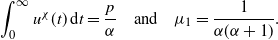
We will also need
 $\mu_1 = \int_0^{\infty} t \nu_{\alpha}({\textrm{d}} t)<\infty$
, the first moment of the probability measure
$\mu_1 = \int_0^{\infty} t \nu_{\alpha}({\textrm{d}} t)<\infty$
, the first moment of the probability measure
 $\nu_\alpha$
.
$\nu_\alpha$
.
The characteristic
 $\chi$
enables us to count quantities in the population. The characteristic counting process
$\chi$
enables us to count quantities in the population. The characteristic counting process
 $Z^\chi$
is defined as
$Z^\chi$
is defined as
 \begin{equation*}Z^{\chi}\!(t) = \sum_{\textbf{i} \in \Sigma} \chi_\textbf{i} (t - \sigma_\textbf{i}).\end{equation*}
There is a recursive decomposition of
 $Z^\chi$
,
$Z^\chi$
,
 \begin{equation*} Z^{\chi}\!(t) = \sum_{\textbf{i} \in \Sigma} \chi_\textbf{i} (t - \sigma_\textbf{i}) = \chi_\emptyset(t) +\sum_{i = 1}^{\xi_\emptyset(\infty)} Z_i^\chi(t- \sigma_i),\end{equation*}
where the
 $Z^\chi_i$
are i.i.d. copies of
$Z^\chi_i$
are i.i.d. copies of
 $Z^\chi$
.
$Z^\chi$
.
To state the strong law of large numbers for the process
 $Z^{\chi}$
we require two more quantities. Firstly we define the discounted mean process and the discounted mean characteristic
$Z^{\chi}$
we require two more quantities. Firstly we define the discounted mean process and the discounted mean characteristic
 \begin{equation*}z^{\chi}\!(t) = {\textrm{e}}^{-\alpha t} \mathbb{E} Z^{\chi}\!(t) \quad \text{and} \quad u^{\chi}\!(t) = {\textrm{e}}^{-\alpha t} \mathbb{E} \chi(t).\end{equation*}
It is easy to check that these satisfy the renewal equation
 \begin{equation*} z^{\chi}\!(t) = u^{\chi}\!(t) + \int_0^\infty z^\chi(t-s) \nu_\alpha({\textrm{d}} s).\end{equation*}
The second quantity we require is the analogue of the classical branching process martingale defined by
 \begin{equation*} M_t = \sum_{\textbf{i} \in \Lambda_t} {\textrm{e}}^{-\alpha \sigma_\textbf{i}}, \end{equation*}
where
 \begin{equation*} \Lambda_t = \{\textbf{i}\in\Sigma\,:\, \textbf{i} = \textbf{j} i \mbox{ for some }\textbf{j}\in\Sigma,i\in\mathbb N,\mbox{ and }\sigma_{\textbf{j}}\leq t < \sigma_\textbf{i}\} \end{equation*}
is the set of individuals born after time t to parents born up to time t. The process M is a non-negative càdlàg
 $\mathcal F_t$
-martingale with unit expectation, where
$\mathcal F_t$
-martingale with unit expectation, where
 \begin{equation*}\mathcal F_t = \sigma(\mathcal F_\textbf{i}, \sigma_\textbf{i} \leq t) \quad\text{and} \quad \mathcal F_\textbf{i} = \sigma(\{(\xi_\textbf{j}, L_\textbf{j})\,:\,\sigma_\textbf{j} \leq \sigma_\textbf{i}\}).\end{equation*}
As M is a positive martingale, by the martingale convergence theorem,
 $M_t \to M_\infty$
as
$M_t \to M_\infty$
as
 $t \to \infty$
, almost surely, for some random variable
$t \to \infty$
, almost surely, for some random variable
 $M_\infty$
. Furthermore, under the condition that
$M_\infty$
. Furthermore, under the condition that
 $\mathbb{E} [\xi_\gamma(\infty) (\!\log \xi_\gamma(\infty))_+ ] < \infty$
, the martingale M is uniformly integrable, there is
$\mathbb{E} [\xi_\gamma(\infty) (\!\log \xi_\gamma(\infty))_+ ] < \infty$
, the martingale M is uniformly integrable, there is
 $L^1$
convergence
$L^1$
convergence
 $M_t\to M_{\infty}$
, and the limit random variable is non-degenerate in that
$M_t\to M_{\infty}$
, and the limit random variable is non-degenerate in that
 $0<M_{\infty}<\infty$
almost surely.
$0<M_{\infty}<\infty$
almost surely.
We now give a less general version (Theorem 2.5 in [Reference Charmoy, Croydon and Hambly13], coupled with the comments in the paragraph preceding the statement of the theorem) of Nerman’s theorem, a strong law for the general branching process counted with characteristic
 $\chi$
, suitable for our purposes.
$\chi$
, suitable for our purposes.
Theorem 2.1. Let
 $(\xi_\textbf{i}, \chi_\textbf{i})_\textbf{i}$
be a general branching process with Malthusian parameter
$(\xi_\textbf{i}, \chi_\textbf{i})_\textbf{i}$
be a general branching process with Malthusian parameter
 $\alpha$
, where
$\alpha$
, where
 $\chi \geq 0$
and
$\chi \geq 0$
and
 $\chi(t) = 0$
for
$\chi(t) = 0$
for
 $t < 0$
. Assume that
$t < 0$
. Assume that
 $\nu_\alpha$
is non-lattice. Assume further that
$\nu_\alpha$
is non-lattice. Assume further that
 $\mathbb{E} \xi(\infty)<\infty$
and there exists a non-increasing bounded positive integrable càdlàg function h on
$\mathbb{E} \xi(\infty)<\infty$
and there exists a non-increasing bounded positive integrable càdlàg function h on
 $[0, \infty)$
such that
$[0, \infty)$
such that
 \begin{equation*} \mathbb{E} \biggl( \sup_{t \geq 0} \frac{{\textrm{e}}^{-\alpha t} \chi(t)}{h(t)} \biggr) < \infty. \end{equation*}
Then
 \begin{equation*} z^{\chi}\!(t) \to z^\chi(\infty) = \mu_1^{-1}{\int_0^\infty u^\chi(s) \,{\textrm{d}} s} \end{equation*}
and
 \begin{equation*} {\textrm{e}}^{-\alpha t} Z^{\chi}\!(t) \to z^\chi(\infty) M_\infty, \quad a.s., \end{equation*}
as
 $t \to \infty$
, where
$t \to \infty$
, where
 $M_\infty$
is the almost sure positive limit of the fundamental martingale of the general branching process. Furthermore, if
$M_\infty$
is the almost sure positive limit of the fundamental martingale of the general branching process. Furthermore, if
 $\mathbb{E} [\xi_\gamma(\infty) (\!\log \xi_\gamma(\infty))_+ ]< \infty$
, the convergence also takes place in
$\mathbb{E} [\xi_\gamma(\infty) (\!\log \xi_\gamma(\infty))_+ ]< \infty$
, the convergence also takes place in
 $L^1$
.
$L^1$
.
2.2. General branching random walks
To discuss the GBRW in
 $\mathbb{R}^d$
we include the spatial component to the general branching process. Here we give a theorem about the growth and spread of such processes.
$\mathbb{R}^d$
we include the spatial component to the general branching process. Here we give a theorem about the growth and spread of such processes.
It is a classical result that a supercritical branching process will grow exponentially and that a supercritical branching random walk will have an associated shape theorem which indicates the region in which the number of particles will grow exponentially. Here we quote a result from Biggins [Reference Biggins9] in the d-dimensional case. A full version of the one-dimensional case is stated and proved in [Reference Biggins8].
Firstly we need to define some terms. The moment generating function for the positions and birth times of the offspring (note that in our case they will have paired atoms) is
 \begin{equation*} m(\boldsymbol{\theta},\phi) = \mathbb{E} \int {\textrm{e}}^{-\boldsymbol{\theta}. \textbf{x}-\phi t} \eta_{\emptyset}({\textrm{d}} \textbf{x})\xi_{\emptyset}({\textrm{d}} t),\quad \boldsymbol{\theta}\in {\mathbb R}^d,\ \phi \in {\mathbb R}_+. \end{equation*}
We assume that
 $m(\boldsymbol{\theta},\phi)<\infty$
in a neighbourhood of the origin. We set
$m(\boldsymbol{\theta},\phi)<\infty$
in a neighbourhood of the origin. We set
 \begin{equation*} \alpha(\boldsymbol{\theta}) = \inf\{ \phi\,:\, m(\boldsymbol{\theta},\phi) \leq 1\}, \end{equation*}
and set
 $\alpha^*$
to be the Legendre transform defined by
$\alpha^*$
to be the Legendre transform defined by
 \begin{equation*} \alpha^*(\textbf{a}) = \inf_{\boldsymbol{\theta}}\{ \textbf{a}.\boldsymbol{\theta} + \alpha(\boldsymbol{\theta})\}. \end{equation*}
We write
 ${\mathcal A} \,:\!=\, \operatorname{int}\{ \textbf{a}\,:\, \alpha^*(\textbf{a})>-\infty\}$
.
${\mathcal A} \,:\!=\, \operatorname{int}\{ \textbf{a}\,:\, \alpha^*(\textbf{a})>-\infty\}$
.
Let
 $Z^{\chi}_t$
denote the random measure consisting of point masses at the locations of the individuals counted according to the characteristic
$Z^{\chi}_t$
denote the random measure consisting of point masses at the locations of the individuals counted according to the characteristic
 $\chi$
at time t:
$\chi$
at time t:
 \begin{equation*} Z^{\chi}_t = \sum_{\textbf{i}\in T} \delta_{z_{\textbf{i}}} \chi_{\textbf{i}}(t-\sigma_{\textbf{i}}). \end{equation*}
Thus if
 $\chi_{\textbf{i}}(t) = I_{\{\sigma_{\textbf{i}}<t\}}$
, then
$\chi_{\textbf{i}}(t) = I_{\{\sigma_{\textbf{i}}<t\}}$
, then
 $Z^{\chi}_t\!(A)$
is the number of individuals that have been in the set A by time t. The characteristic
$Z^{\chi}_t\!(A)$
is the number of individuals that have been in the set A by time t. The characteristic
 $\chi_{\textbf{i} j} = I_{\{\sigma_\textbf{i} < t, \sigma_{\textbf{i} j}\geq t\}}$
gives the process that records the locations of the individuals in the coming generation at time t. We will see that this captures the rectangles that arise from splitting rectangles of area larger then
$\chi_{\textbf{i} j} = I_{\{\sigma_\textbf{i} < t, \sigma_{\textbf{i} j}\geq t\}}$
gives the process that records the locations of the individuals in the coming generation at time t. We will see that this captures the rectangles that arise from splitting rectangles of area larger then
 ${\textrm{e}}^{-t}$
, but not yet splitting ones of smaller area.
${\textrm{e}}^{-t}$
, but not yet splitting ones of smaller area.
Definition 2.1. A process is said to be well-regulated if
 \begin{equation*} \mathbb{E} \sup_t {\textrm{e}}^{-\alpha(\theta) t} \chi_{\emptyset}(t) < \infty. \end{equation*}
It has exponential tails if for any unit vector
 $\textbf{n}$
there are
$\textbf{n}$
there are
 $\boldsymbol{\theta},\phi$
such that
$\boldsymbol{\theta},\phi$
such that
 $m(\textbf{n}.\boldsymbol{\theta},\phi)<\infty$
.
$m(\textbf{n}.\boldsymbol{\theta},\phi)<\infty$
.
We say that the process is lattice if the spatial location of the offspring is confined to lie on a discrete subgroup of
 $\mathbb R^d$
.
$\mathbb R^d$
.
Theorem 2.2. ([Reference Biggins9, Theorem 4.1].) Suppose that the process with the characteristic
 $\chi$
is well-regulated, non-lattice, and has exponential tails. Suppose that A is a closed convex set with a non-empty interior such that
$\chi$
is well-regulated, non-lattice, and has exponential tails. Suppose that A is a closed convex set with a non-empty interior such that
 $\operatorname{int}\!(A)\cap {\mathcal A}\neq \emptyset$
. Let
$\operatorname{int}\!(A)\cap {\mathcal A}\neq \emptyset$
. Let
 $\beta = \sup\{\alpha^*(a)\,:\, a\in A\}$
.
$\beta = \sup\{\alpha^*(a)\,:\, a\in A\}$
.
-
(i) If
$\beta<0$
, then for any
$\gamma>\beta$
\begin{equation*} {\textrm{e}}^{-\gamma t} Z^{\chi}_t\!(tA) \to 0, \quad t\to\infty, \quad a.s. \end{equation*}
-
(ii) If
$\beta>0$
, then
\begin{equation*} t^{-1}\log Z^{\chi}_t\!(tA) \to \beta, \quad t\to\infty,\quad a.s. \end{equation*}


In the problem at hand the spatial locations and birth times of offspring will have full support in
 $\mathbb R^{d+1}_+$
and hence the non-lattice condition is fulfilled. The other conditions will also follow straightforwardly in our application. Thus we should see exponential growth of the number of individuals at points in the interior of the region where
$\mathbb R^{d+1}_+$
and hence the non-lattice condition is fulfilled. The other conditions will also follow straightforwardly in our application. Thus we should see exponential growth of the number of individuals at points in the interior of the region where
 $\beta>0$
. Unfortunately this theorem is not directly applicable, as we will see that, for our model where we split the largest rectangle first, the function
$\beta>0$
. Unfortunately this theorem is not directly applicable, as we will see that, for our model where we split the largest rectangle first, the function
 $\alpha^*(a)$
is only finite on a line segment in
$\alpha^*(a)$
is only finite on a line segment in
 $\mathbb{R}^2$
, and thus we will extend this theorem to cover the situation where the offspring lie in a space–time hyperplane, as occurs in our model.
$\mathbb{R}^2$
, and thus we will extend this theorem to cover the situation where the offspring lie in a space–time hyperplane, as occurs in our model.
We also note that there are more refined theorems in less general settings, for instance in [Reference Biggins7] and [Reference Uchiyama32] and a large subsequent literature for discrete time branching processes, Markov branching processes, branching diffusions, and fragmentation processes.
3. Power laws for interfaces
We will now consider the lengths of horizontal interfaces in a complete fragmentation of the unit square. Let
 $N^p_h(x)$
denote the number of horizontal interfaces in the unit square that are of length greater than or equal to x when the probability of horizontal edges is p. It is a simple observation that if
$N^p_h(x)$
denote the number of horizontal interfaces in the unit square that are of length greater than or equal to x when the probability of horizontal edges is p. It is a simple observation that if
 $p>1/2$
, this quantity will be infinite with positive probability, as there is a positive probability that the number of edges of unit length goes to infinity, as the number of edges of unit length is a supercritical Galton–Watson branching process. In the case where
$p>1/2$
, this quantity will be infinite with positive probability, as there is a positive probability that the number of edges of unit length goes to infinity, as the number of edges of unit length is a supercritical Galton–Watson branching process. In the case where
 $p=1/2$
, the random variable
$p=1/2$
, the random variable
 $N^p_h(x)$
has infinite mean and we will not discuss it further. As a result we will only consider the case
$N^p_h(x)$
has infinite mean and we will not discuss it further. As a result we will only consider the case
 $p<1/2$
, and we will see that
$p<1/2$
, and we will see that
 $N^p_h(x)$
is almost surely finite and will give a limit theorem for its scaling with x.
$N^p_h(x)$
is almost surely finite and will give a limit theorem for its scaling with x.
In order to do this we introduce a suitable general branching process. As we are tracking the number of horizontal edges of a certain size, if a rectangle is split in the horizontal direction, that will correspond to having a horizontal edge of exactly the same length as the parent and two new rectangles which could produce more horizontal edges of the same size. A split in the vertical direction will lead to new rectangles that will produce edges of smaller length. To map this into a general branching process we will set
 $x={\textrm{e}}^{-t}$
, where t is time. Then
$x={\textrm{e}}^{-t}$
, where t is time. Then
 $Z^{\chi}_t = N^p_h({\textrm{e}}^{-t})$
is a general branching process (for a suitable
$Z^{\chi}_t = N^p_h({\textrm{e}}^{-t})$
is a general branching process (for a suitable
 $\chi$
) in which an individual’s offspring distribution will either be two offspring born at the same time as the parent, or two at later times given as
$\chi$
) in which an individual’s offspring distribution will either be two offspring born at the same time as the parent, or two at later times given as
 ${-}\log{U}$
and
${-}\log{U}$
and
 ${-}\log\!{(1-U)}$
for U a uniform random variable on [0, 1]. The general branching process structure is able to handle this instantaneous birth process.
${-}\log\!{(1-U)}$
for U a uniform random variable on [0, 1]. The general branching process structure is able to handle this instantaneous birth process.
We define the birth point process
 $\xi$
using U, a U[0, 1]-random variable, and B, a Bernoulli(p) random variable, as
$\xi$
using U, a U[0, 1]-random variable, and B, a Bernoulli(p) random variable, as
 \begin{equation*} \xi({\textrm{d}} t) = 2I_{B=1}\delta_{0}({\textrm{d}} t) + I_{B=0}(\delta_{-\log{U}}({\textrm{d}} t)+\delta_{-\log\!{(1-U)}}({\textrm{d}} t)). \end{equation*}
The counting function
 $\chi$
is used to capture the number of horizontal edges of length at least
$\chi$
is used to capture the number of horizontal edges of length at least
 ${\textrm{e}}^{-t}$
produced by an individual and is thus given by
${\textrm{e}}^{-t}$
produced by an individual and is thus given by
 $\chi(t) = I_{B=1}$
, for
$\chi(t) = I_{B=1}$
, for
 $t\geq 0$
, as the only time we produce a horizontal interface is with a horizontal split.
$t\geq 0$
, as the only time we produce a horizontal interface is with a horizontal split.
We write
 \begin{equation*} Z^{\chi}(t) = \sum_{\textbf{i} \in \Sigma} \chi_{\textbf{i}}(t-\sigma_{\textbf{i}}), \end{equation*}
so that
 $Z^{\chi}(t)$
counts all the edges of length greater than
$Z^{\chi}(t)$
counts all the edges of length greater than
 ${\textrm{e}}^{-t}$
. Theorem 2.1 shows that, provided there are not too many offspring too far in the future, there will be a strong law of large numbers for this process. We first find the Malthusian parameter
${\textrm{e}}^{-t}$
. Theorem 2.1 shows that, provided there are not too many offspring too far in the future, there will be a strong law of large numbers for this process. We first find the Malthusian parameter
 $\alpha$
as the solution to
$\alpha$
as the solution to
 \begin{equation*}1 = \mathbb{E} \sum_{i=1}^{\xi(\infty)} {\textrm{e}}^{-\alpha\sigma_i} = 2p + (1-p)\dfrac{2}{\alpha+1}.\end{equation*}
That is, the Malthusian parameter is given by
 $\alpha = 1/(1-2p)$
.
$\alpha = 1/(1-2p)$
.
Recalling the notation from the section on the general branching process, we then set
 \begin{equation*} z^{\chi}(t) = {\textrm{e}}^{-\alpha t} \mathbb{E} Z^{\chi}(t) \end{equation*}
and
 \begin{equation*} u^{\chi}(t) = {\textrm{e}}^{-\alpha t} \mathbb{E} \chi(t) = {\textrm{e}}^{-\alpha t} p. \end{equation*}
The fundamental martingale M, determined by the weighted birth times of the coming generation, is
 \begin{equation*} M_t = \sum_{\textbf{i} j\,:\, \sigma_{\textbf{i}}\leq t< \sigma_{\textbf{i} j}} {\textrm{e}}^{-\alpha \sigma_{\textbf{i} j}}. \end{equation*}
Theorem 3.1. For the counting process
 $Z^{\chi}(t)$
we have
$Z^{\chi}(t)$
we have
 \begin{equation*} \lim_{t\to \infty} {\textrm{e}}^{-\alpha t} Z^{\chi}(t) =\dfrac{\alpha^2-1}{2\alpha} M_{\infty}, \quad a.s., \end{equation*}
where
 $M_{\infty} = \lim_{t\to\infty} M_t$
exists and is non-degenerate.
$M_{\infty} = \lim_{t\to\infty} M_t$
exists and is non-degenerate.
Proof. In order to apply Theorem 2.1, the strong law of large numbers for the general branching process, we need to check the conditions. Firstly observe that the family size is always 2 and hence finite and the measure
 $\nu_{\alpha}$
is non-lattice. The characteristic
$\nu_{\alpha}$
is non-lattice. The characteristic
 $\chi$
is non-decreasing in t as it is constant with
$\chi$
is non-decreasing in t as it is constant with
 $\mathbb{E}\chi(\infty) = p<\infty$
and hence, taking the decreasing, integrable function
$\mathbb{E}\chi(\infty) = p<\infty$
and hence, taking the decreasing, integrable function
 $h(t)=\exp\!({-}\epsilon t)$
for
$h(t)=\exp\!({-}\epsilon t)$
for
 $\epsilon<\alpha$
, in the conditions of Theorem 2.1, we have
$\epsilon<\alpha$
, in the conditions of Theorem 2.1, we have
 \begin{equation*} \mathbb{E} \biggl( \sup_{t \geq 0} {\textrm{e}}^{-(\alpha-\epsilon) t} \chi(t) \biggr) \leq \mathbb{E}\chi(\infty) = p<\infty. \end{equation*}
Thus we can apply the theorem, and all we need is to compute the limit in the renewal equation. This is
 \begin{equation*} \lim_{t\to\infty} z^{\chi}(t) = \dfrac1{\mu_1}\int_0^{\infty} u^{\chi}(t) \,{\textrm{d}} t, \end{equation*}
where
 $\mu_1 = \mathbb{E} \int_0^{\infty} t {\textrm{e}}^{-\alpha t} \xi({\textrm{d}} t)$
. Standard calculations give
$\mu_1 = \mathbb{E} \int_0^{\infty} t {\textrm{e}}^{-\alpha t} \xi({\textrm{d}} t)$
. Standard calculations give
 \begin{equation*}\int_0^{\infty} u^{\chi}(t) \,{\textrm{d}} t = \frac{p}{\alpha}\quad \text{and}\quad\mu_1 =\frac{1}{\alpha(\alpha+1)}.\end{equation*}
Putting these two results together, and using
 $p=(\alpha-1)/2\alpha$
, we have the result.
$p=(\alpha-1)/2\alpha$
, we have the result.
Remark 3.1. In order to avoid instantaneous births, we could look at all the offspring produced at the one time point as being from the offspring distribution of a general branching process. Thus an individual born at time t will have a collection of offspring at the two times
 $t-\log{U}$
and
$t-\log{U}$
and
 $t-\log\!{(1-U)}$
. The offspring distributions at these times are given by two independent random variables which can each be written as
$t-\log\!{(1-U)}$
. The offspring distributions at these times are given by two independent random variables which can each be written as
 $(T_0+1)/2$
, where
$(T_0+1)/2$
, where
 $T_0$
is the time for a simple random walk on
$T_0$
is the time for a simple random walk on
 $\mathbb{Z}_+$
with upsteps of probability p to hit 0 from 1.
$\mathbb{Z}_+$
with upsteps of probability p to hit 0 from 1.
As a corollary, by making the time transformation that
 $t=-\log{x}$
, we have our power law limit theorem.
$t=-\log{x}$
, we have our power law limit theorem.
Theorem 3.2. There exists a strictly positive mean-one random variable
 $M_{\infty}$
such that
$M_{\infty}$
such that
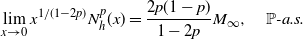 \begin{equation*} \lim_{x\to 0} x^{1/(1-2p)}N^p_h(x) = \dfrac{2p(1-p)}{1-2p} M_{\infty}, \quad \textit{$\mathbb{P}$-a.s.} \end{equation*}
Remark 3.2. (1) An analogous fragmentation mechanism for a lattice with finite spacing has been described in [Reference Torrens, Illa, Vives and Planes31]. It is shown that in the limit as the lattice spacing vanishes, the mean of the distribution of interfaces of length greater than or equal to x tends to a power law with exponent
 ${{1}/{(1-2p)}}$
as in the present study.
${{1}/{(1-2p)}}$
as in the present study.
(2) If we have
 $p=0$
, this limit is 0, corresponding to the fact that there are no horizontal interfaces!
$p=0$
, this limit is 0, corresponding to the fact that there are no horizontal interfaces!
Remark 3.3. (1) The three-dimensional case of the model enables us to compute the exponent without requiring bias. Let
 $N_h(a)$
denote the number of horizontal interfaces of area at least a; then, setting
$N_h(a)$
denote the number of horizontal interfaces of area at least a; then, setting
 $a={\textrm{e}}^{-t}$
, we will have a general branching process as in the two-dimensional case. Now, if there is a horizontal slice, we produce an interface with that area. When we split in a different direction the horizontal area is uniformly split into two pieces. Thus we have exactly the same GBP as before but now the natural probability is
$a={\textrm{e}}^{-t}$
, we will have a general branching process as in the two-dimensional case. Now, if there is a horizontal slice, we produce an interface with that area. When we split in a different direction the horizontal area is uniformly split into two pieces. Thus we have exactly the same GBP as before but now the natural probability is
 $1/3$
, as this is the probability of a horizontal split. Directly applying our previous result, we see that
$1/3$
, as this is the probability of a horizontal split. Directly applying our previous result, we see that
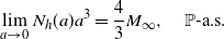 \begin{equation*} \lim_{a\to 0} N_h(a) a^{3} = \dfrac43 M_{\infty},\quad \text{$\mathbb{P}$-a.s.} \end{equation*}
Thus we have Theorem 1.1.
(2) The power law result is a function of the whole fragmentation, and the time parameter used to generate the fragmentation has no impact on this.
3.1. Tail estimates for
$\boldsymbol{M}_{\boldsymbol\infty}$

We conclude with some analysis of the limit random variable
 $M_{\infty}$
. In the setting of the classical Galton–Watson branching process, the left and right tail asymptotics have been studied; see for instance [Reference Biggins and Bingham10]. In the case of the general branching process for the left and right tail there are results in [Reference Hambly and Jones18] in the case where the probability space of outcomes is finite. In the context of multiplicative cascades, estimates on the left and right tails in a similar case to the one considered here can be found in [Reference Liu21] and [Reference Liu22]. Our general branching process does not fit into these frameworks and it is not clear how to apply their techniques, so we deduce slightly weaker results in our setting.
$M_{\infty}$
. In the setting of the classical Galton–Watson branching process, the left and right tail asymptotics have been studied; see for instance [Reference Biggins and Bingham10]. In the case of the general branching process for the left and right tail there are results in [Reference Hambly and Jones18] in the case where the probability space of outcomes is finite. In the context of multiplicative cascades, estimates on the left and right tails in a similar case to the one considered here can be found in [Reference Liu21] and [Reference Liu22]. Our general branching process does not fit into these frameworks and it is not clear how to apply their techniques, so we deduce slightly weaker results in our setting.
3.1.1. The right tail.
We obtain an upper bound for the right tail. A key observation is that, by [Reference Gatzouras16, Theorem 3.3], the limit random variable
 $M_{\infty}$
satisfies the following equation after conditioning on the first event. For ease of notation we now write
$M_{\infty}$
satisfies the following equation after conditioning on the first event. For ease of notation we now write
 $M, M_1, M_2$
for independent copies of
$M, M_1, M_2$
for independent copies of
 $M_{\infty}$
, giving
$M_{\infty}$
, giving
 \begin{equation} M = (M_1+M_2)I_{B=1} + (M_1U^{\alpha} + M_2(1-U)^{\alpha})I_{B=0},\end{equation}
where
 $U\sim U[0, 1]$
, and
$U\sim U[0, 1]$
, and
 $B=1$
if the split is horizontal and
$B=1$
if the split is horizontal and
 $B=0$
if the split is vertical. Let
$B=0$
if the split is vertical. Let
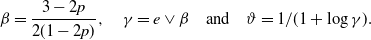 \begin{equation*}\beta = \frac{3-2p}{2(1-2p)},\quad \gamma=e\vee \beta\quad\text{and}\quad\vartheta=1/(1+\log{\gamma}).\end{equation*}
Theorem 3.3. There exists a constant
 $c_1$
such that for all
$c_1$
such that for all
 $\lambda>1$
 \begin{equation*} \mathbb{P}(M_{\infty}>\lambda) \leq c_1 \lambda^{\vartheta/2+1} \exp\!({-} \lambda^{\vartheta}). \end{equation*}
In order to prove this, as there is no control on the maximum growth rate, which can be used in the case where there are only a finite number of outcomes as in [Reference Hambly and Jones18], we estimate the moment growth.
Lemma 3.1. We have
 \begin{equation*} \mathbb{E}(M^k) \leq k!\gamma^{k\log{k}} \quad for\ all \ k\in \mathbb{N}. \end{equation*}
Proof. We take expectations using (3.1) to get
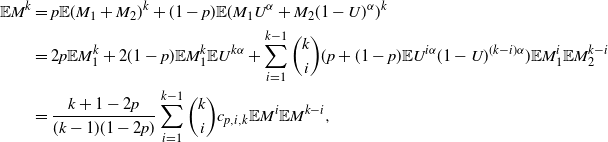 \begin{align*}\mathbb{E}M^k &= p\mathbb{E}(M_1+M_2)^k + (1-p)\mathbb{E}(M_1U^{\alpha}+M_2(1-U)^{\alpha})^k \\ &= 2p\mathbb{E} M_1^k + 2(1-p) \mathbb{E}M_1^k\mathbb{E} U^{k\alpha} + \sum_{i=1}^{k-1} \binom{k}{i}(p+(1-p)\mathbb{E}U^{i\alpha}(1-U)^{(k-i)\alpha} ) \mathbb{E} M_1^i \mathbb{E} M_2^{k-i} \\ &= \dfrac{k+1-2p}{(k-1)(1-2p)} \sum_{i=1}^{k-1} \binom{k}{i} c_{p,i,k} \mathbb{E}M^i \mathbb{E}M^{k-i},\end{align*}
where
 $c_{p,i,k} = p+(1-p)B(i\alpha +1,(k-i)\alpha+1)$
and B is the beta function. It is easy to see from the integral formula for the beta function that
$c_{p,i,k} = p+(1-p)B(i\alpha +1,(k-i)\alpha+1)$
and B is the beta function. It is easy to see from the integral formula for the beta function that
 $B(i\alpha+1,(k-i)\alpha+1) \leq 1/(\alpha+1)$
for all
$B(i\alpha+1,(k-i)\alpha+1) \leq 1/(\alpha+1)$
for all
 $1\leq i\leq k-1$
and
$1\leq i\leq k-1$
and
 $k\geq 2$
. As a result we have that
$k\geq 2$
. As a result we have that
 $p\leq c_{p,i,k} \leq 1/2$
for all
$p\leq c_{p,i,k} \leq 1/2$
for all
 $0\leq p<1/2$
and
$0\leq p<1/2$
and
 $1\leq i \leq k-1$
.
$1\leq i \leq k-1$
.
Now setting
 $a_k = \mathbb{E} M^k/k!$
, we have the following recurrence:
$a_k = \mathbb{E} M^k/k!$
, we have the following recurrence:
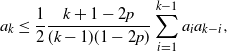 \begin{equation*} a_k \leq \dfrac12 \dfrac{k+1-2p}{(k-1)(1-2p)} \sum_{i=1}^{k-1} a_i a_{k-i}, \end{equation*}
with
 $a_1=1$
. We note that
$a_1=1$
. We note that
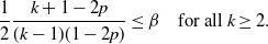 \begin{equation*}\frac12 \frac{k+1-2p}{(k-1)(1-2p)} \leq \beta \quad\text{for all $k\geq 2$.}\end{equation*}
The proof will be complete if we can show
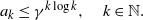 \begin{equation} a_k \leq \gamma^{k\log{k}}, \quad k\in\mathbb{N}.\end{equation}
We use induction. We have the result for
 $k=1$
and now assume it for all
$k=1$
and now assume it for all
 $i\leq k-1$
. Then
$i\leq k-1$
. Then
 \begin{equation*} a_k \leq \beta \sum_{i=1}^{k-1} \gamma^{i\log{i} + (k-i)\log\!(k-i)}. \end{equation*}
As the function in the exponent is convex, its maximum will occur at
 $i=1$
or
$i=1$
or
 $i=k-1$
, and we have
$i=k-1$
, and we have
 \begin{equation*} a_k \leq \beta (k-1) \gamma^{(k-1)\log\!{(k-1)}}. \end{equation*}
Taking logs, we see
 \begin{equation*} \log{a_k} \leq (k-1)\log\!{(k-1)}\log{\gamma} + \log\!{(k-1)} +\log{\beta} = k\log{k}\log{\gamma} + R_k, \end{equation*}
where
 \begin{equation*} R_k = k(\!\log\!{(k-1)}-\log{k})\log{\gamma} + (1-\log{\gamma})\log\!{(k-1)} + \log{\beta}. \end{equation*}
We show that
 $R_k\leq 0$
. As
$R_k\leq 0$
. As
 $\log\!{(1-1/k)} \leq -1/k$
, we have
$\log\!{(1-1/k)} \leq -1/k$
, we have
 \begin{equation*} R_k \leq -\log{\gamma} + (1-\log{\gamma})\log\!{(k-1)} + \log{\beta}. \end{equation*}
Thus if
 $\gamma=e$
we have
$\gamma=e$
we have
 $R_k\leq \log{\beta}-1 \leq 0$
as
$R_k\leq \log{\beta}-1 \leq 0$
as
 $\beta\leq e$
, while if
$\beta\leq e$
, while if
 $\gamma=\beta$
we have
$\gamma=\beta$
we have
 $\log{\beta}\geq 1$
and then
$\log{\beta}\geq 1$
and then
 $R_k \leq (1-\log{\beta})\log\!{(k-1)}\leq 0$
. Hence we have (3.2) and the proof of Lemma 3.1 follows.
$R_k \leq (1-\log{\beta})\log\!{(k-1)}\leq 0$
. Hence we have (3.2) and the proof of Lemma 3.1 follows.
An application of Stirling’s formula gives the following.
Corollary 3.1. There exists a constant
 $c_2$
such that for all
$c_2$
such that for all
 $k\in\mathbb{N}$
 \begin{equation*} \mathbb{E}M^k \leq c_2 k^{1/2} \exp\!{((1+\log{\gamma})k\log{k} - k)}. \end{equation*}
Proof of Theorem
3.3.By Markov’s inequality and Corollary 3.1, we have for all
 $\lambda>0$
 \begin{align*} \mathbb{P}(M>\lambda) &\leq \mathbb{E}M^k \lambda^{-k}\\ &\leq c_2 k^{1/2} \lambda^{-k} {\textrm{e}}^{(1+\log{\gamma})k\log{k}-k}. \end{align*}
As this holds for all
 $k\in \mathbb{N}$
, for
$k\in \mathbb{N}$
, for
 $\lambda>1$
we choose k such that
$\lambda>1$
we choose k such that
 $k\leq \lambda^{\vartheta} <k+1$
, where
$k\leq \lambda^{\vartheta} <k+1$
, where
 $\vartheta=1/(1+\log{\gamma})$
.
$\vartheta=1/(1+\log{\gamma})$
.
Now we note that
 $\log{k} \leq \vartheta \log{\lambda}$
and
$\log{k} \leq \vartheta \log{\lambda}$
and
 $\lambda^{\vartheta}-1 \leq k \leq \lambda^{\vartheta}$
. Thus for
$\lambda^{\vartheta}-1 \leq k \leq \lambda^{\vartheta}$
. Thus for
 $\lambda>1$
we have
$\lambda>1$
we have
 \begin{align*}P(M>\lambda) &\leq c_2 \lambda^{\vartheta/2} \exp\!({-}(\lambda^{\vartheta}-1)\log{\lambda} + (1+\log{\gamma})\vartheta\lambda^{\vartheta}\log{\lambda}-\lambda^{\vartheta}+1) \\&= c_2 \lambda^{\vartheta/2} \exp\!(\!\log{\lambda}-\lambda^{\vartheta} +1) \\&= c_2e \lambda^{\vartheta/2+1}{\textrm{e}}^{-\lambda^{\vartheta}},\end{align*}
as required.
We note that if
 $p<(2e-3)/4e-2)\approx 0.275$
, then
$p<(2e-3)/4e-2)\approx 0.275$
, then
 $\beta<e$
and
$\beta<e$
and
 $\vartheta=1/2$
. Also
$\vartheta=1/2$
. Also
 $\vartheta\to 0$
as
$\vartheta\to 0$
as
 $p\to 1/2$
.
$p\to 1/2$
.
3.1.2. The left tail.
In order to estimate the left tail of the probability distribution we will need to understand the case where the growth rate is slow. This corresponds to the event that there are many vertical splits of the square so that the population in the general branching process has offspring later and hence grows more slowly. The minimal growth rate will therefore occur when every split is a vertical one. Thus, to emphasize that we are dealing with vertical division only, we write
 $\Lambda^{\prime}_t$
for the collection of children alive after time t of mothers born before time t in this case. We first note that as we are just splitting the unit interval, this corresponds to the case when
$\Lambda^{\prime}_t$
for the collection of children alive after time t of mothers born before time t in this case. We first note that as we are just splitting the unit interval, this corresponds to the case when
 $p=0$
, hence
$p=0$
, hence
 $\alpha=1$
and the associated fundamental martingale
$\alpha=1$
and the associated fundamental martingale
 $M^0_t \equiv 1$
for all
$M^0_t \equiv 1$
for all
 $t\geq 0$
.
$t\geq 0$
.
Lemma 3.2. We have the following bound for all
 $\omega\in \Omega$
:
$\omega\in \Omega$
:
 \begin{equation*} |\Lambda^{\prime}_t| \geq {\textrm{e}}^t \quad for\ all\ t\geq 0. \end{equation*}
Proof. We observe that for
 $\textbf{i}\in\Lambda^{\prime}_t$
we have
$\textbf{i}\in\Lambda^{\prime}_t$
we have
 $\sigma_{\textbf{i}}>t$
. Hence, for all
$\sigma_{\textbf{i}}>t$
. Hence, for all
 $t\geq 0$
,
$t\geq 0$
,
 \begin{equation*} 1= M^0_t = \sum_{\textbf{i}\in\Lambda^{\prime}_t} {\textrm{e}}^{-\sigma_{\textbf{i}}} \leq |\Lambda^{\prime}_t| {\textrm{e}}^{- t}, \end{equation*}
as required.
Let
 $\Lambda_t^c = \{\textbf{i}\in\Lambda^{\prime}_t\,:\, \sigma_\textbf{i} \leq t+c \}$
denote the offspring born between t and
$\Lambda_t^c = \{\textbf{i}\in\Lambda^{\prime}_t\,:\, \sigma_\textbf{i} \leq t+c \}$
denote the offspring born between t and
 $t+c$
of mothers born before t.
$t+c$
of mothers born before t.
Corollary 3.2. We have that, for all
 $\omega\in\Omega$
,
$\omega\in\Omega$
,
 \begin{equation*} |\Lambda_t^{\log{2}}| \geq \dfrac{1}{2} {\textrm{e}}^t \quad for\ all\ t>0. \end{equation*}
Proof. As offspring are born at
 ${-}\log{U}$
and
${-}\log{U}$
and
 ${-}\log\!{(1-U)}$
for
${-}\log\!{(1-U)}$
for
 $U\in [0, 1]$
, we observe that any parent born before t with children after time t must have at least one offspring before time
$U\in [0, 1]$
, we observe that any parent born before t with children after time t must have at least one offspring before time
 $t+\log{2}$
of their birth. Thus there must be at least half the offspring within t to
$t+\log{2}$
of their birth. Thus there must be at least half the offspring within t to
 $t+\log{2}$
.
$t+\log{2}$
.
There is an almost sure convergence result for this minimal growth rate.
Lemma 3.3. We have that
 \begin{equation*} |\Lambda^{\prime}_t|{\textrm{e}}^{-t} \to 2, \quad a.s. \quad as\ \text{$ t\to\infty$.} \end{equation*}
Proof. We apply the law of large numbers in Theorem 2.1 and compute, in the case where
 $p=0$
, that
$p=0$
, that
 $\mu_1=1/2$
. In order to count the coming generation we use the characteristic
$\mu_1=1/2$
. In order to count the coming generation we use the characteristic
 $\chi(t) = I_{\{\sigma_1>t\}}+I_{\{\sigma_2>t\}}$
, as this counts the children of a parent appearing after time t. Thus the value of
$\chi(t) = I_{\{\sigma_1>t\}}+I_{\{\sigma_2>t\}}$
, as this counts the children of a parent appearing after time t. Thus the value of
 $u^{\chi}(t) = 2{\textrm{e}}^{-2t}$
and we can compute the limit in the theorem as given, recalling that
$u^{\chi}(t) = 2{\textrm{e}}^{-2t}$
and we can compute the limit in the theorem as given, recalling that
 $M^0_{\infty}=1$
.
$M^0_{\infty}=1$
.
Now that we have established the minimal growth rate we can apply a standard approach to estimating the left tail.
Let
 $\phi(u) = \mathbb{E}\exp\!({-}uM_{\infty})$
denote the Laplace transform of
$\phi(u) = \mathbb{E}\exp\!({-}uM_{\infty})$
denote the Laplace transform of
 $M_{\infty}$
. As the random variables
$M_{\infty}$
. As the random variables
 $M_{\infty}$
are non-degenerate, the Laplace transform is a continuous decreasing function of u with
$M_{\infty}$
are non-degenerate, the Laplace transform is a continuous decreasing function of u with
 $\phi(0)=1$
and
$\phi(0)=1$
and
 $\phi(u)>0$
, for all
$\phi(u)>0$
, for all
 $u>0$
, and
$u>0$
, and
 $\phi(u)\to 0$
as
$\phi(u)\to 0$
as
 $u\to\infty$
.
$u\to\infty$
.
We consider splitting the process according to
 $\Lambda_t$
, in which case
$\Lambda_t$
, in which case
 \begin{equation*} M_{\infty} = \sum_{\textbf{i}\in\Lambda_t} {\textrm{e}}^{-\alpha \sigma_{\textbf{i}}} M_{\infty,\textbf{i}}, \end{equation*}
where
 $M_{\infty,\textbf{i}}$
are independent copies of
$M_{\infty,\textbf{i}}$
are independent copies of
 $M_{\infty}$
. Therefore the Laplace transform satisfies
$M_{\infty}$
. Therefore the Laplace transform satisfies
 \begin{equation*} \phi(u) = \mathbb{E} \prod_{\textbf{i}\in\Lambda_t} \phi(u{\textrm{e}}^{-\alpha\sigma_{\textbf{i}}}). \end{equation*}
We now give bounds on the Laplace transform of
 $M_{\infty}$
.
$M_{\infty}$
.
Theorem 3.4. There exist strictly positive constants
 $c_i$
,
$c_i$
,
 $i=3,4,5,6$
such that for all
$i=3,4,5,6$
such that for all
 $u> 0$
 \begin{equation*} c_3\exp\bigl({-}c_4 u^{1/\alpha}\bigr) \leq \phi(u) \leq c_5\exp\bigl({-}c_6 u^{1/\alpha}\bigr). \end{equation*}
Proof. We begin with the upper bound. By definition for
 $\textbf{i}\in\Lambda^{\log{2}}_t$
we have
$\textbf{i}\in\Lambda^{\log{2}}_t$
we have
 $t<\sigma_{\textbf{i}}\leq t+\log{2}$
. Hence for
$t<\sigma_{\textbf{i}}\leq t+\log{2}$
. Hence for
 $\textbf{i}\in\Lambda_t^{\log{2}}$
we have
$\textbf{i}\in\Lambda_t^{\log{2}}$
we have
 \begin{equation*} \phi(u{\textrm{e}}^{-\alpha \sigma_{\textbf{i}}}) \leq \phi(u{\textrm{e}}^{-\alpha t}2^{-\alpha}) \end{equation*}
and
 \begin{equation*} \phi(u) \leq \mathbb{E} \prod_{\textbf{i}\in\Lambda_t^c} \phi(u{\textrm{e}}^{-\alpha\sigma_{\textbf{i}}}) \leq \mathbb{E} \phi(u{\textrm{e}}^{-\alpha t}2^{-\alpha})^{|\Lambda_t^{\log{2}}|}. \end{equation*}
Thus by Corollary 3.2 we have
 \begin{equation} \phi(u) \leq \phi(u{\textrm{e}}^{-\alpha t}2^{-\alpha})^{\frac12 {\textrm{e}}^t} \quad \text{for all $t>0$.}\end{equation}
Now we use this result to extend a bound over a compact interval to the whole of
 $u\geq 1$
. As
$u\geq 1$
. As
 $\phi$
is continuous, decreasing with
$\phi$
is continuous, decreasing with
 $\phi(0)=1$
, we can find
$\phi(0)=1$
, we can find
 $\hat{c}>0$
such that for
$\hat{c}>0$
such that for
 $1\leq u \leq {\textrm{e}}^{\alpha}$
we have the initial bound
$1\leq u \leq {\textrm{e}}^{\alpha}$
we have the initial bound
 \begin{equation*} \phi(u) \leq {\textrm{e}}^{-\hat{c} u^{1/\alpha}}. \end{equation*}
If
 $u\in [{\textrm{e}}^{\alpha n}2^{\alpha}, {\textrm{e}}^{\alpha (n+1)}2^{\alpha}]$
, for an integer
$u\in [{\textrm{e}}^{\alpha n}2^{\alpha}, {\textrm{e}}^{\alpha (n+1)}2^{\alpha}]$
, for an integer
 $n>0$
we have
$n>0$
we have
 $u{\textrm{e}}^{-\alpha n}2^{-\alpha} \in [1,{\textrm{e}}^{\alpha}]$
, and thus by (3.3)
$u{\textrm{e}}^{-\alpha n}2^{-\alpha} \in [1,{\textrm{e}}^{\alpha}]$
, and thus by (3.3)
 \begin{equation*} \phi(u) \leq \exp\biggl({-}\hat{c} (u{\textrm{e}}^{-\alpha n}2^{-\alpha})^{1/\alpha}\dfrac12 {\textrm{e}}^n\biggr) = \exp\bigl({-}\hat{c}2^{-2} u^{1/\alpha}\bigr). \end{equation*}
This bound holds for all
 $n>0$
and hence we have it for all
$n>0$
and hence we have it for all
 $u\geq 1$
. We can extend to all
$u\geq 1$
. We can extend to all
 $u\geq 0$
by adjusting the leading constant.
$u\geq 0$
by adjusting the leading constant.
For the lower bound we note that
 $\sigma_{\textbf{i}} \leq t$
for
$\sigma_{\textbf{i}} \leq t$
for
 $\sigma\in\Lambda^{\prime}_t$
and observe that, by considering the probability of the pure vertical splitting, we have
$\sigma\in\Lambda^{\prime}_t$
and observe that, by considering the probability of the pure vertical splitting, we have
 \begin{align*}\phi(u) &= \mathbb{E} \prod_{\textbf{i}\in\Lambda_t} \phi(u{\textrm{e}}^{-\alpha\sigma_{\textbf{i}}}) \\ &\geq \mathbb{E} \Biggl( (1-p)^{|\Lambda^{\prime}_t|} \prod_{\textbf{i}\in\Lambda^{\prime}_t}\phi(u{\textrm{e}}^{-\alpha t}) \Biggr) \\ & \geq \mathbb{E} \bigl( (1-p)^{|\Lambda^{\prime}_t|} \phi(u{\textrm{e}}^{-\alpha t})^{|\Lambda^{\prime}_t|}; |\Lambda^{\prime}_t| \leq 3 {\textrm{e}}^t \bigr) \\ & \geq ( (1-p)\phi(u{\textrm{e}}^{-\alpha t}))^{3{\textrm{e}}^t}\mathbb{P}(|\Lambda^{\prime}_t| \leq 3 {\textrm{e}}^t).\end{align*}
Now as
 $|\Lambda^{\prime}_t|{\textrm{e}}^{-t}$
converges to the constant 2 almost surely by Lemma 3.3, there is a constant
$|\Lambda^{\prime}_t|{\textrm{e}}^{-t}$
converges to the constant 2 almost surely by Lemma 3.3, there is a constant
 $c_0$
such that
$c_0$
such that
 $\mathbb{P}(|\Lambda^{\prime}_t| \leq 3 {\textrm{e}}^t)\geq c_0$
for all
$\mathbb{P}(|\Lambda^{\prime}_t| \leq 3 {\textrm{e}}^t)\geq c_0$
for all
 $t>0$
. We conclude that
$t>0$
. We conclude that
 \begin{equation} \phi(u) \geq c_0( (1-p)\phi(u{\textrm{e}}^{-\alpha t}))^{3{\textrm{e}}^t}.\end{equation}
As for the upper bound we use the continuity properties of
 $\phi$
to obtain an initial bound: that there is a constant
$\phi$
to obtain an initial bound: that there is a constant
 $\hat{c}_1$
such that
$\hat{c}_1$
such that
 \begin{equation*} \phi(u) \geq {\textrm{e}}^{-\hat{c}_1 u^{1/\alpha}}, \quad u\in [1,{\textrm{e}}^{\alpha}]. \end{equation*}
Now consider
 $u \in [{\textrm{e}}^{\alpha n}, {\textrm{e}}^{\alpha (n+1)}]$
for some integer
$u \in [{\textrm{e}}^{\alpha n}, {\textrm{e}}^{\alpha (n+1)}]$
for some integer
 $n>0$
. We see that for this n we have
$n>0$
. We see that for this n we have
 ${\textrm{e}}^{-\alpha n} u \in [1,{\textrm{e}}^{\alpha}]$
and
${\textrm{e}}^{-\alpha n} u \in [1,{\textrm{e}}^{\alpha}]$
and
 ${\textrm{e}}^n\leq u^{1/\alpha}$
. Hence for this u, by (3.4), we have
${\textrm{e}}^n\leq u^{1/\alpha}$
. Hence for this u, by (3.4), we have
 \begin{equation*} \phi(u) \geq c_0 (1-p)^{3 u^{1/\alpha}} {\textrm{e}}^{-\hat{c}_1(u{\textrm{e}}^{-\alpha n})^{1/\alpha}3{\textrm{e}}^n} \geq c_0 \exp\bigl({-}3(\!\log\!{(1/(1-p))}+\hat{c}_1)u^{1/\alpha}\bigr). \end{equation*}
As
 $0\leq p<1/2$
, the bound holds for all
$0\leq p<1/2$
, the bound holds for all
 $n>0$
with constant
$n>0$
with constant
 $c_4=3(\!\log\!{(1/(1-p))}+\hat{c}_1)$
and hence for all
$c_4=3(\!\log\!{(1/(1-p))}+\hat{c}_1)$
and hence for all
 $u\geq 1$
with this
$u\geq 1$
with this
 $c_4$
. By adjusting the leading constant, we have the result for all
$c_4$
. By adjusting the leading constant, we have the result for all
 $u>0$
.
$u>0$
.
We are now ready for our tail estimates.
Theorem 3.5. There exist strictly positive constants
 $c_i$
for
$c_i$
for
 $i=7,8,9,10$
such that for
$i=7,8,9,10$
such that for
 $\lambda>0$
 \begin{equation*} c_7 \exp\bigl({-}c_8 \lambda^{-1/(\alpha-1)}\bigr) \leq \mathbb{P}(M_{\infty} < \lambda) \leq c_{9} \exp\bigl({-}c_{10} \lambda^{-1/(\alpha-1)}\bigr). \end{equation*}
Proof. For the upper bound we use a standard exponential bound approach,
 \begin{align*}\mathbb{P}(M_{\infty} < \lambda) &\leq \exp\!(u\lambda)\phi(u) \\&\leq c_5 \exp\bigl(u\lambda - c_6 u^{1/\alpha}\bigr).\end{align*}
As this holds for all
 $u>0$
, we can optimize by setting
$u>0$
, we can optimize by setting
 $u=(\lambda\alpha/c_6)^{\alpha/(1-\alpha)}$
to get the upper bound with
$u=(\lambda\alpha/c_6)^{\alpha/(1-\alpha)}$
to get the upper bound with
 $c_{10} = (\alpha-1)(c_6/\alpha)^{\alpha/(\alpha-1)}.$
For the lower bound we observe that
 \begin{align*}\phi(u) &= \mathbb{E} {\textrm{e}}^{-uM_{\infty}}I_{\{M_{\infty}<\lambda\}} + \mathbb{E} {\textrm{e}}^{-uM_{\infty}}I_{\{M_{\infty}\geq \lambda \}}\\&\leq \mathbb{P}(M_{\infty}<\lambda) + {\textrm{e}}^{-u\lambda}(1-\mathbb{P}(M_{\infty}<\lambda)).\end{align*}
Hence
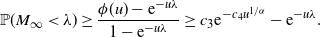 \begin{equation*} \mathbb{P}(M_{\infty}<\lambda) \geq \dfrac{\phi(u)-{\textrm{e}}^{-u\lambda}}{1-{\textrm{e}}^{-u\lambda}} \geq c_3{\textrm{e}}^{-c_4u^{1/\alpha}} - {\textrm{e}}^{-u\lambda}. \end{equation*}
Now noting that
 $c_3<1$
, if we choose
$c_3<1$
, if we choose
 $u=\xi \lambda^{-\alpha/(\alpha-1)}$
, where
$u=\xi \lambda^{-\alpha/(\alpha-1)}$
, where
 $\xi$
satisfies
$\xi$
satisfies
 $\xi-\log\!{(2/c_3)} =c_4 \xi^{1/\alpha}$
(and which is easily seen to be positive), then
$\xi-\log\!{(2/c_3)} =c_4 \xi^{1/\alpha}$
(and which is easily seen to be positive), then
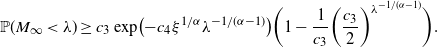 \begin{equation*} \mathbb{P}(M_{\infty}<\lambda) \geq c_3\exp\bigl({-}c_4\xi^{1/\alpha} \lambda^{-1/(\alpha-1)}\bigr)\biggl(1-\dfrac{1}{c_3}\biggl(\dfrac{c_3}{2}\biggr)^{\lambda^{-1/(\alpha-1)}} \biggr). \end{equation*}
Thus for
 $\lambda<1$
we have
$\lambda<1$
we have
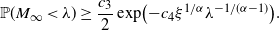 \begin{equation*} \mathbb{P}(M_{\infty}<\lambda) \geq \dfrac{c_3}{2} \exp\bigl({-}c_4\xi^{1/\alpha} \lambda^{-1/(\alpha-1)}\bigr). \end{equation*}
The leading constants can be adjusted to obtain the estimates over all
 $\lambda>0$
.
$\lambda>0$
.
4. Asymptotics of rectangles
Our initial analysis focused on the power law behaviour of interfaces in a complete fragmentation. The focus in this section is to include a time parameter to study the asymptotics of interfaces arising from small rectangles. In order to do this we encode the model as a general branching random walk in
 $\mathbb R^2_+$
, where each individual corresponds to a rectangle with their location determined by its side lengths.
$\mathbb R^2_+$
, where each individual corresponds to a rectangle with their location determined by its side lengths.
We recall the description of the labelled tree from Section 2. To describe our fragmentation for each vertex
 $\textbf{i}$
in the tree we have a pair
$\textbf{i}$
in the tree we have a pair
 $(U_{\textbf{i}},B_{\textbf{i}})$
, where
$(U_{\textbf{i}},B_{\textbf{i}})$
, where
 $U_{\textbf{i}}$
is a uniformly distributed random variable over [0, 1] determining the random division of the rectangle, and
$U_{\textbf{i}}$
is a uniformly distributed random variable over [0, 1] determining the random division of the rectangle, and
 $B_{\textbf{i}}$
is a Bernoulli(p), for
$B_{\textbf{i}}$
is a Bernoulli(p), for
 $0<p<1$
, random variable which determines whether the interface is horizontal or vertical, so
$0<p<1$
, random variable which determines whether the interface is horizontal or vertical, so
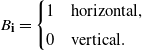 \begin{equation*} B_{\textbf{i}} = \begin{cases} 1 & \text{horizontal,} \\[3pt] 0 & \text{vertical.} \end{cases} \end{equation*}
Using this we can write the two possible outcomes from splitting a rectangle (a, b) with index
 $\textbf{i}$
as two new rectangles
$\textbf{i}$
as two new rectangles
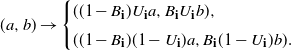 \begin{equation*} (a,b) \to \begin{cases} ((1-B_{\textbf{i}})U_{\textbf{i}}a,B_{\textbf{i}}U_{\textbf{i}}b), \\[3pt]((1-B_{\textbf{i}})(1-U_{\textbf{i}})a,B_{\textbf{i}}(1-U_{\textbf{i}})b). \end{cases} \end{equation*}
At this stage there is no time parameter; the tree provides a description of all the fragmentations. We now consider two possible time parametrizations. In the first we split the rectangles to ensure that at a given time all rectangles are at most a certain size. In the second every rectangle evolves independently of the rest, the splitting time occurring at a constant rate.
4.1. Splitting largest areas first
In our first approach we ensure the rectangles in the pattern are of roughly the same size at a given time by taking the birth time of the individual to be determined by their size. To incorporate the branching structure we will make a logarithmic transformation of the coordinate system. In this way all the individuals alive at time t correspond to rectangles with areas that are at most
 ${\textrm{e}}^{-t}$
.
${\textrm{e}}^{-t}$
.
In order to convert this into a GBRW we regard each rectangle as an individual with a location given by the logarithm of the side lengths of the rectangle. We also introduce a time coordinate in order to ensure that the larger rectangles split before the smaller ones, and do this using the space and time distribution of the offspring of individual
 $\textbf{i}$
:
$\textbf{i}$
:
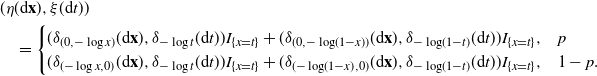 \begin{align*} & (\eta({\textrm{d}} \textbf{x}),\xi({\textrm{d}} t)) \\ & \quad = \begin{cases} (\delta_{(0,-\log{x})}({\textrm{d}} \textbf{x}), \delta_{{-\log{t}}}({\textrm{d}} t))I_{\{x=t\}} + (\delta_{(0,-\log\!{(1-x)})}({\textrm{d}} \textbf{x}),\delta_{-\log\!{(1-t)}}({\textrm{d}} t)) I_{\{x=t\}}, & p \\ (\delta_{({-}\log{x},0)}({\textrm{d}} \textbf{x}),\delta_{{-\log{t}}}({\textrm{d}} t))I_{\{x=t\}} + (\delta_{({-}\log\!{(1-x)},0)}({\textrm{d}} \textbf{x}), \delta_{-\log\!{(1-t)}}({\textrm{d}} t)) I_{\{x=t\}}, & 1-p . \end{cases} \end{align*}
Thus we can view this evolution as the individual has two offspring which are both born in a location displaced from their parent by a shift in either the x or y coordinate directions. The time of their births is determined by how far they are displaced. Note that the first birth can be thought of as the time of division of the rectangle but the smaller rectangle is coded by the parent until the time of the second birth, when we may think of the parent dying, and this second offspring is then able to divide.
The associated general branching random walk is the point process of individuals in the population at their respective locations at time t. Each individual reproduces independently according to the point process above. We observe that this offspring distribution lies on a space–time hyperplane
 $x+y=t$
, and this will lead us to develop an extension to Theorem 2.2. We now proceed to do the concrete calculations for the interface model we have here in order to see why we need to extend Theorem 2.2. We recall the definitions from Section 2.2 and begin by computing
$x+y=t$
, and this will lead us to develop an extension to Theorem 2.2. We now proceed to do the concrete calculations for the interface model we have here in order to see why we need to extend Theorem 2.2. We recall the definitions from Section 2.2 and begin by computing
 $m(\boldsymbol{\theta},\phi)$
, where
$m(\boldsymbol{\theta},\phi)$
, where
 $\boldsymbol{\theta} = (\theta_1,\theta_2)$
, as
$\boldsymbol{\theta} = (\theta_1,\theta_2)$
, as
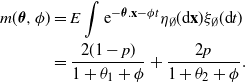 \begin{align*} m(\boldsymbol{\theta},\phi) &= E \int {\textrm{e}}^{-\boldsymbol{\theta}. \textbf{x}-\phi t} \eta_{\emptyset}({\textrm{d}} \textbf{x})\xi_{\emptyset}({\textrm{d}} t) \\ &= \dfrac{2(1-p)}{1+\theta_1+\phi} + \dfrac{2p}{1+\theta_2+\phi}.\end{align*}
Note that this is finite for
 $(\boldsymbol{\theta},\phi) \in \{ \theta_1,\theta_2,\phi\,:\, \theta_1+\phi>-1, \theta_2+\phi>-1\}$
.
$(\boldsymbol{\theta},\phi) \in \{ \theta_1,\theta_2,\phi\,:\, \theta_1+\phi>-1, \theta_2+\phi>-1\}$
.
Then we can find
 $\alpha(\boldsymbol{\theta})$
as
$\alpha(\boldsymbol{\theta})$
as
 \begin{align*}\alpha(\boldsymbol{\theta}) &= \inf\{\phi\,:\, m(\boldsymbol{\theta},\phi)\leq 1\} \\&= \inf\{\phi\,:\, \phi^2 + (\theta_1+\theta_2)\phi +\theta_1\theta_2+(2p-1)(\theta_2-\theta_1)-1 \geq 0 \}.\end{align*}
Thus by continuity we can solve the quadratic and take the smallest root over the set where
 $m(\boldsymbol{\theta},\phi)$
is defined, to get
$m(\boldsymbol{\theta},\phi)$
is defined, to get
 \begin{equation*} \alpha(\boldsymbol{\theta}) = -\dfrac12(\theta_1+\theta_2) + \dfrac12 \sqrt{(\theta_1-\theta_2)^2+4(2p-1)(\theta_1-\theta_2)+4}. \end{equation*}
Note that
 $\alpha(\boldsymbol{\theta})$
exists for all
$\alpha(\boldsymbol{\theta})$
exists for all
 $\boldsymbol{\theta} \in \mathbb R^2$
and that it is positive for all
$\boldsymbol{\theta} \in \mathbb R^2$
and that it is positive for all
 $\theta_1+\theta_2<0$
.
$\theta_1+\theta_2<0$
.
We now wish to determine the Legendre transform
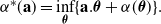 \begin{equation*} \alpha^*(\textbf{a}) = \inf_{\boldsymbol{\theta}}\{ \textbf{a}.\boldsymbol{\theta} + \alpha(\boldsymbol{\theta})\}. \end{equation*}
At this point it is useful to change variables and set
 $\varphi=\theta_1+\theta_2$
and
$\varphi=\theta_1+\theta_2$
and
 $\psi=\theta_1-\theta_2$
with
$\psi=\theta_1-\theta_2$
with
 $\varphi,\psi\in\mathbb R$
. Thus our function to minimize becomes
$\varphi,\psi\in\mathbb R$
. Thus our function to minimize becomes
 \begin{equation*}\textbf{a}.\boldsymbol{\theta} + \alpha(\boldsymbol{\theta})= \dfrac12 \varphi(a_1+a_2-1) + \dfrac12 (a_1-a_2)\psi + \dfrac12 \sqrt{\psi^2+4(2p-1)\psi+4}.\end{equation*}
Hence, if
 $a_1+a_2-1\neq 0$
, the infimum is
$a_1+a_2-1\neq 0$
, the infimum is
 $-\infty$
by taking
$-\infty$
by taking
 $\varphi\to \pm \infty$
. If we have
$\varphi\to \pm \infty$
. If we have
 $a_1+a_2-1=0$
, then we are left with an equation in
$a_1+a_2-1=0$
, then we are left with an equation in
 $\psi$
which we can minimize to get
$\psi$
which we can minimize to get
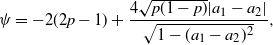 \begin{equation*} \psi = -2(2p-1)+\dfrac{4\sqrt{p(1-p)}|a_1-a_2|}{\sqrt{1-(a_1-a_2)^2}}, \end{equation*}
and hence
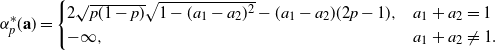 \begin{equation*} \alpha_p^*(\textbf{a}) = \begin{cases} 2\sqrt{p(1-p)}\sqrt{1-(a_1-a_2)^2} - (a_1-a_2)(2p-1), & a_1+a_2=1 \\ -\infty, & a_1+a_2 \neq 1. \end{cases}\end{equation*}
In the case where
 $p=1/2$
, this is
$p=1/2$
, this is
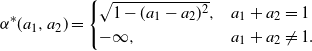 \begin{equation} \alpha^*(a_1,a_2) = \begin{cases} \sqrt{1-(a_1-a_2)^2}, & a_1+a_2 = 1 \\-\infty, & a_1+a_2\neq 1. \end{cases}\end{equation}
That is, for
 $0\leq a_1 \leq 1$
we have
$0\leq a_1 \leq 1$
we have
 \begin{equation*} \alpha^*(a_1,1-a_1) = 2\sqrt{a_1(1-a_1)} = 2\sqrt{a_1a_2} \end{equation*}
and
 $\alpha^*(a_1,a_2)=-\infty$
for all other values of
$\alpha^*(a_1,a_2)=-\infty$
for all other values of
 $\textbf{a}=(a_1,a_2)$
.
$\textbf{a}=(a_1,a_2)$
.
Unfortunately, as
 $\alpha^*(\textbf{a})$
is only finite on a closed set with empty interior, we cannot apply Theorem 2.2 directly. However, it is not difficult to extend the theorem to the situation where the offspring distribution lives on a hyperplane in space–time as we have here. We will consider the more general case where the offspring distribution in
$\alpha^*(\textbf{a})$
is only finite on a closed set with empty interior, we cannot apply Theorem 2.2 directly. However, it is not difficult to extend the theorem to the situation where the offspring distribution lives on a hyperplane in space–time as we have here. We will consider the more general case where the offspring distribution in
 $\mathbb{R}^d \times \mathbb{R}_+$
could lie in the hyperplane
$\mathbb{R}^d \times \mathbb{R}_+$
could lie in the hyperplane
 $\sum_{i=1}^d w_i x_i = t$
, where
$\sum_{i=1}^d w_i x_i = t$
, where
 $w_i\in\mathbb{R}$
are constants. We could follow the same idea if the hyperplane were of dimension
$w_i\in\mathbb{R}$
are constants. We could follow the same idea if the hyperplane were of dimension
 $k<d-1$
, but here we just consider the
$k<d-1$
, but here we just consider the
 $(d-1)$
-dimensional case, as in our model the hyperplane is
$(d-1)$
-dimensional case, as in our model the hyperplane is
 $x_1+x_2=t$
.
$x_1+x_2=t$
.
We let
 $\tilde{\mathcal{A}}$
be the interior of
$\tilde{\mathcal{A}}$
be the interior of
 $\{\textbf{a}\,:\, \alpha^*(\textbf{a})>-\infty\}$
considered as a
$\{\textbf{a}\,:\, \alpha^*(\textbf{a})>-\infty\}$
considered as a
 $(d-1)$
-dimensional subset of
$(d-1)$
-dimensional subset of
 $\mathbb{R}^d$
. For any Borel set
$\mathbb{R}^d$
. For any Borel set
 $A\subset \mathbb{R}^d$
, we let
$A\subset \mathbb{R}^d$
, we let
 $N_t(A)$
denote the number of individuals in A at time t.
$N_t(A)$
denote the number of individuals in A at time t.
Theorem 4.1. Suppose that A is a closed convex set in
 $\mathbb R^d$
with a non-empty interior.
$\mathbb R^d$
with a non-empty interior.
-
(i) If
$A \cap\tilde{\mathcal{A}}=\emptyset$
, then
\begin{equation*} t^{-1} \log{N_t(tA)} \to -\infty, \quad t\to\infty, \quad a.s. \end{equation*}
-
(ii) If
$A \cap\tilde{\mathcal{A}}\neq \emptyset$
, then setting
$\beta = \sup\{\alpha^*(\textbf{a})\,:\, \textbf{a}\in A\}$
we have
\begin{equation*} t^{-1}\log N_t(tA) \to \beta, \quad t\to\infty,\quad a.s. \end{equation*}


Proof. In order to prove this theorem we show how to apply Theorem 4.1 of [Reference Biggins9]. As the offspring distribution lies on a hyperplane we can rotate the coordinates so that this hyperplane is parallel to
 $x_1=0$
. This aligns the first space coordinate with time and reduces the problem to one in
$x_1=0$
. This aligns the first space coordinate with time and reduces the problem to one in
 $\mathbb{R}^{d-1}$
. We let
$\mathbb{R}^{d-1}$
. We let
 $\textbf{y}=R_{\vartheta}\textbf{x}$
be the rotation so that
$\textbf{y}=R_{\vartheta}\textbf{x}$
be the rotation so that
 $y_1 = \sum_i w_i x_i$
and hence
$y_1 = \sum_i w_i x_i$
and hence
 $y_1=t$
. Then we have that the d-dimensional moment generating function can be expressed in terms of a
$y_1=t$
. Then we have that the d-dimensional moment generating function can be expressed in terms of a
 $(d-1)$
-dimensional one:
$(d-1)$
-dimensional one:
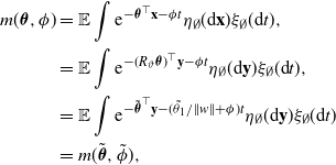 \begin{align*} m(\boldsymbol{\theta}, \phi) &= \mathbb{E} \int {\textrm{e}}^{-\boldsymbol{\theta}^{\top} \textbf{x}-\phi t} \eta_{\emptyset}({\textrm{d}} \textbf{x})\xi_{\emptyset}({\textrm{d}} t), \\&= \mathbb{E} \int {\textrm{e}}^{-(R_{\vartheta} \boldsymbol{\theta})^{\top} \textbf{y}-\phi t} \eta_{\emptyset}({\textrm{d}} \textbf{y})\xi_{\emptyset}({\textrm{d}} t), \\&= \mathbb{E} \int {\textrm{e}}^{-\tilde{\boldsymbol{\theta}}^{\top} \textbf{y}-(\tilde{\theta}_1/\|w\|+\phi) t} \eta_{\emptyset}({\textrm{d}} \textbf{y})\xi_{\emptyset}({\textrm{d}} t) \\&= m(\tilde{\boldsymbol{\theta}}, \tilde{\phi}),\end{align*}
where
 $R_{\vartheta}\boldsymbol{\theta}=(\tilde{\theta}_1, \tilde{\boldsymbol{\theta}})$
, with
$R_{\vartheta}\boldsymbol{\theta}=(\tilde{\theta}_1, \tilde{\boldsymbol{\theta}})$
, with
 $\tilde{\boldsymbol{\theta}}$
the
$\tilde{\boldsymbol{\theta}}$
the
 $(d-1)$
-dimensional vector obtained from removing the first coordinate from
$(d-1)$
-dimensional vector obtained from removing the first coordinate from
 $R_{\vartheta}\boldsymbol{\theta}$
and
$R_{\vartheta}\boldsymbol{\theta}$
and
 $\tilde{\phi} = \phi+\tilde{\theta}_1/\|w\|$
. Thus setting
$\tilde{\phi} = \phi+\tilde{\theta}_1/\|w\|$
. Thus setting
 \begin{equation}\alpha(\boldsymbol{\theta}) = \inf\{\phi\,:\, m(\boldsymbol{\theta},\phi) \leq 1\},\end{equation}
we can calculate
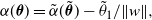 \begin{equation*} \alpha(\boldsymbol{\theta}) = \tilde{\alpha}(\tilde{\boldsymbol{\theta}}) - \tilde{\theta}_1/\|w\|, \end{equation*}
where
 $\tilde{\alpha}$
is computed in the same way as
$\tilde{\alpha}$
is computed in the same way as
 $\alpha$
in (4.2) using
$\alpha$
in (4.2) using
 $m(\tilde{\boldsymbol{\theta}}, \tilde{\phi})$
as a function over the
$m(\tilde{\boldsymbol{\theta}}, \tilde{\phi})$
as a function over the
 $d-1$
variables
$d-1$
variables
 $\tilde{\boldsymbol{\theta}}$
. Computing the Legendre transform we get, writing
$\tilde{\boldsymbol{\theta}}$
. Computing the Legendre transform we get, writing
 $\tilde{\textbf{a}}$
for the
$\tilde{\textbf{a}}$
for the
 $d-1$
coordinates of the
$d-1$
coordinates of the
 $\mathbb{R}^d$
vector
$\mathbb{R}^d$
vector
 $R_{\vartheta}\textbf{a}$
obtained by excluding the first coordinate, and
$R_{\vartheta}\textbf{a}$
obtained by excluding the first coordinate, and
 $\tilde{\alpha}^*$
for the Legendre transform of
$\tilde{\alpha}^*$
for the Legendre transform of
 $\tilde{\alpha}$
,
$\tilde{\alpha}$
,
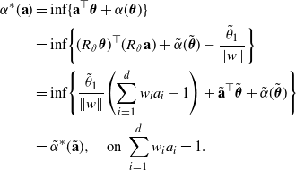 \begin{align}\alpha^*(\textbf{a}) &= \inf\{ \textbf{a}^{\top}\boldsymbol{\theta} + \alpha(\boldsymbol{\theta})\} \notag \\&= \inf\biggl\{(R_{\vartheta}\boldsymbol{\theta})^{\top} (R_{\vartheta} \textbf{a}) + \tilde{\alpha}(\tilde{\boldsymbol{\theta}})-\dfrac{\tilde{\theta}_1}{\|w\|} \biggr\} \notag \\&= \inf\Biggl\{\dfrac{\tilde{\theta}_1}{\|w\|}\Biggl(\sum_{i=1}^d w_i a_i -1\Biggr) + \tilde{\textbf{a}}^{\top} \tilde{\boldsymbol{\theta}} + \tilde{\alpha}(\tilde{\boldsymbol{\theta}})\Biggr\} \notag \\&= \tilde{\alpha}^{*}(\tilde{\textbf{a}}), \quad\text{on }\sum_{i=1}^d w_i a_i = 1. \end{align}
We now establish the limit result for the growth of the number of particles in the set A. By using the rotation
 $R_{\vartheta}$
, we have
$R_{\vartheta}$
, we have
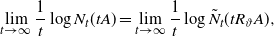 \begin{equation*} \lim_{t\to\infty} \dfrac{1}{t} \log{N_t(tA)} = \lim_{t\to\infty} \dfrac{1}{t} \log{\tilde{N}_t(tR_{\vartheta}A)}, \end{equation*}
where
 $\tilde{N}_t$
is the number of individuals in the rotated GBRW. Now consider the last
$\tilde{N}_t$
is the number of individuals in the rotated GBRW. Now consider the last
 $d-1$
coordinates of this rotated process, which is the GBRW in
$d-1$
coordinates of this rotated process, which is the GBRW in
 $\mathbb{R}^{d-1}$
with offspring distribution whose spatial steps are given by
$\mathbb{R}^{d-1}$
with offspring distribution whose spatial steps are given by
 $Y_i, i=2,\dots,d$
, where
$Y_i, i=2,\dots,d$
, where
 $Y=R_{\vartheta}X$
. We can apply Theorem 2.2 to this process to obtain the result in
$Y=R_{\vartheta}X$
. We can apply Theorem 2.2 to this process to obtain the result in
 $\mathbb{R}^{d-1}$
with Legendre transform
$\mathbb{R}^{d-1}$
with Legendre transform
 $\tilde{\alpha}^*$
. Using (4.3), undoing the rotation, we can write this back in terms of
$\tilde{\alpha}^*$
. Using (4.3), undoing the rotation, we can write this back in terms of
 $\alpha^*$
, and we see that the limit results hold for our original branching process in
$\alpha^*$
, and we see that the limit results hold for our original branching process in
 $\mathbb{R}^d$
.
$\mathbb{R}^d$
.
Theorem 1.2 now follows from Theorem 4.1 by setting
 $p=1/2$
and transforming the function
$p=1/2$
and transforming the function
 $\alpha^*$
in (4.1) to the original coordinates to obtain
$\alpha^*$
in (4.1) to the original coordinates to obtain
 $\gamma^*$
as given. Note that we can apply Theorem 4.1 to the analogous three-dimensional version of the model, but it does not appear to lead to an analytically tractable Legendre transform.
$\gamma^*$
as given. Note that we can apply Theorem 4.1 to the analogous three-dimensional version of the model, but it does not appear to lead to an analytically tractable Legendre transform.
4.2. Splitting independently
Our calculations so far supposed that we always split the largest rectangles first. An alternative is to choose to split each rectangle independently of the rest. Our approach via a general branching random walk process allows us to use any distribution for the splitting time, but we can obtain more precise limit theorems in the case where the split occurs at constant rate, in which case we have a Markov branching random walk. In this setting small pieces divide in the same way as the large pieces, and this will generally give a much greater disparity in the sizes of the individual rectangles at a given time.
To illustrate we just compute
 $\alpha^*(\textbf{a})$
, the function which determines the asymptotic growth rate in the general branching random walk for the version of the model in which the constant splitting rate is 1 and
$\alpha^*(\textbf{a})$
, the function which determines the asymptotic growth rate in the general branching random walk for the version of the model in which the constant splitting rate is 1 and
 $p=1/2$
.
$p=1/2$
.
The GBRW becomes a Markov branching random walk but we stay within the GBRW framework initially to compute the asymptotic growth rate as before. Firstly the Laplace transform of the offspring birth and location measure is
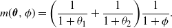 \begin{equation*} m(\boldsymbol{\theta},\phi) = \biggl(\dfrac1{1+\theta_1} +\dfrac{1}{1+\theta_2}\biggr)\dfrac{1}{1+\phi}. \end{equation*}
Hence
 \begin{equation*} \alpha(\boldsymbol{\theta}) = \dfrac1{1+\theta_1} +\dfrac{1}{1+\theta_2} -1. \end{equation*}
The Legendre transform is found by setting
 \begin{equation}\theta_1= a_1^{-1/2}-1, \quad \theta_2 = a_2^{-1/2}-1 ,\end{equation}
which gives
 \begin{equation*} \alpha^*(\textbf{a}) = 1-(1-\sqrt{a_1})^2-(1-\sqrt{a_2})^2, \quad a_1,a_2>0.\end{equation*}
As
 $\alpha^*(\textbf{a})>0$
in an open set we can apply a transformed version of Theorem 2.2. We let
$\alpha^*(\textbf{a})>0$
in an open set we can apply a transformed version of Theorem 2.2. We let
 \begin{equation*} \gamma^*(a,b) = \alpha^*({-}\log{a},-\log{b}) = 1-(1-\sqrt{{-}\log{a}})^2-(1-\sqrt{{-}\log{b}})^2, \quad 0< a,b<1 \end{equation*}
and S be a closed convex set in
 $[0, 1]^2$
. Then for
$[0, 1]^2$
. Then for
 $\beta = \sup_{(a,b)\in S} \gamma^*(a,b)$
we have, if
$\beta = \sup_{(a,b)\in S} \gamma^*(a,b)$
we have, if
 $\beta>0$
,
$\beta>0$
,
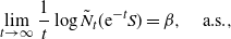 \begin{equation*} \lim_{t\to \infty} \dfrac{1}{t}\log{\tilde{N}_t({\textrm{e}}^{-t}S)} = \beta, \quad \text{a.s.}, \end{equation*}
while if
 $\beta<0$
, then for any
$\beta<0$
, then for any
 $\delta>\beta$
 \begin{equation*} \lim_{t\to\infty} {\textrm{e}}^{-\delta t}\tilde{N}_t({\textrm{e}}^{-t}S) = 0, \quad\text{a.s.} \end{equation*}
In [Reference Uchiyama32] it is shown that for a Markov branching random walk, where the individual gives birth at the moment of their death, there is a finer limit theorem on the growth of the number of individuals in a certain set. In our setting and notation, this gives that for a fixed
 $\textbf{a}$
, such that
$\textbf{a}$
, such that
 $\alpha^*(\textbf{a})>0$
, we have
$\alpha^*(\textbf{a})>0$
, we have
 \begin{equation*} \lim_{t\to\infty} t\exp\!({-}\alpha^*(\textbf{a})t) N_t(t\textbf{a} + D) = \dfrac{a_1^{3/4} a_2^{3/4}}{\pi} \int_D{\textrm{e}}^{\theta_1x+\theta_2y} \,{\textrm{d}} x \,{\textrm{d}} y W_{\textbf{a}}, \quad \text{$\mathbb{P}$-a.s.}, \end{equation*}
for any compact subset D of
 $\mathbb{R}^2_+$
, where
$\mathbb{R}^2_+$
, where
 $W_{\textbf{a}}>0$
is a non-degenerate mean-one random variable and
$W_{\textbf{a}}>0$
is a non-degenerate mean-one random variable and
 $\theta_1,\theta_2$
are as in (4.4).
$\theta_1,\theta_2$
are as in (4.4).
Acknowledgements
We thank Professor John Ball for suggesting the model and Professor Eduard Vives for discussions about the alternative model of [Reference Torrens, Illa, Vives and Planes31]. PC is grateful to Professor Giovanni Zanzotto for insightful discussions. We also thank Dr Robert Niemann for kindly giving us permission to publish the illustrative image in Figure 1. PC is grateful to the hospitality of the Mathematical Institute, University of Oxford. PC holds an honorary appointment at La Trobe University and is a member of GNAMPA.
Funding information
PC has been supported by JSPS KAKENHI, grants JP16K21213, JP19H05131, JP21H00102, and an AiRIMaQ Fellowship.
Competing interests
There were no competing interests to declare which arose during the preparation or publication process of this article.


