


1. Spreading of fake news
In a community, fake news and the like is started by someone and spreads out through interactions between individuals of that community. There are active gullible persons who are willing to believe the fake news and participate in spreading it, and there are persons who hear the fake news and do not react to it, either because they are savvy enough to see through the falsehood or are simply uninterested in spreading news, even when they believe it. One sees this phenomenon too often these days in social media.
We assume that the size of the entire community is n (large), and there are initially  $n-j$
persons who will not participate at any point in spreading the news,
$n-j$
persons who will not participate at any point in spreading the news,  $j - 1$
active gullible persons (potential spreaders), and one person who manufactures the news. The number of those who will not participate at any point in spreading the news remains unchanged throughout, whereas the number of spreaders increases, say to k, at which point there are
$j - 1$
active gullible persons (potential spreaders), and one person who manufactures the news. The number of those who will not participate at any point in spreading the news remains unchanged throughout, whereas the number of spreaders increases, say to k, at which point there are  $j-k$
remaining gullible persons who have not yet heard the news.
$j-k$
remaining gullible persons who have not yet heard the news.
Interactions between members of the community take place over time. If a spreader comes in contact with an active gullible person who has not yet heard the news, the active gullible person is converted into a spreader. Any other interaction has no effect and the picture remains unchanged.
A question of interest is ‘How long does it take until a certain proportion of the community have become spreaders?’ The question is obviously of interest to the media, policy makers, and society at large.
There is quite extensive literature on the spreading of rumors. A classic model is the Maki–Thomson [Reference Maki and Thomson8] model, in which informed participants eventually become stiflers not interested in spreading the rumor. The Maki–Thomson model is also considered as a scenario in epidemiology, sociology, and biosciences [Reference Frauenthal5, Reference Molchanov and Whitmeyer9, Reference Svensson14]. Most studies have focused on the spreading of rumors (or diseases) in continuous time [Reference Belen, Kropat and Weber1, Reference Daley and Kendall2, Reference Pittel12, Reference Watson15]. However, a few sources reverted to discrete-time rumor models [Reference Junior, Machado and Zuluaga6, Reference Pittel11, Reference Sudbury13]. Our discrete-time model is essentially different, as it has no migration out of the spreaders. Also, in our scheme the stiflers play a less active role than in the Maki–Thomson model. Furthermore, we take a distributional view and ask a different kind of question, meant to address the multiple phase transitions that occur over time.
2. Notation
Time (discrete) refers to the number of interactions, that is, the number of times two persons from the community come in contact. This is to be contrasted with the notion of discrete time in [Reference Sudbury13], where the epochs are taken only at the points of change.
The average and variance of the waiting time come in terms of the nth harmonic number of order k, namely  $H_n^{(k)} = \sum_{i=1}^n 1/i^k$
. The following are well-known asymptotic representations for the harmonic numbers of the first two orders:
$H_n^{(k)} = \sum_{i=1}^n 1/i^k$
. The following are well-known asymptotic representations for the harmonic numbers of the first two orders:
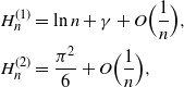 \begin{align}H_n^{(1)} &= \ln n + \gamma+ O\Bigl(\frac 1 {n}\Bigr),\\H_n^{(2)} &= \frac {\pi^2} 6 + O\Bigl(\frac 1 {n}\Bigr),\nonumber\end{align}
where  $\gamma = 0.5772\ldots$
is Euler’s constant. It is customary to suppress the order k when it is 1.
$\gamma = 0.5772\ldots$
is Euler’s constant. It is customary to suppress the order k when it is 1.
There are generalized harmonic numbers with additional parameters. We need a generalized form of the harmonic number of order two, namely
 \begin{equation*}\psi(1, x) = \sum_{i=0}^\infty \frac 1 {(i+x)^2},\end{equation*}
which is also called the trigamma function or Hurwitz zeta function  $\zeta(2, x)$
; see [Reference Whittaker and Watson16, pp. 268--269].
$\zeta(2, x)$
; see [Reference Whittaker and Watson16, pp. 268--269].
We use  ${\rm Geo}(p)$
to indicate a geometric random variable with parameter p. The asymptotic distributions contain a Gumbel distribution. The Gumbel distribution with location parameter
${\rm Geo}(p)$
to indicate a geometric random variable with parameter p. The asymptotic distributions contain a Gumbel distribution. The Gumbel distribution with location parameter  $\theta \in \mathbb R$
and scale parameter
$\theta \in \mathbb R$
and scale parameter  $\beta>0$
has density
$\beta>0$
has density
 \begin{equation*}f(x) = \frac 1 \beta {\rm e}^{-\frac {x-\theta} \beta} {\rm e}^{-{\rm e}^{-\frac {x-\theta} \beta}}, \qquad -\infty <x
< \infty,\end{equation*}
\begin{equation*}f(x) = \frac 1 \beta {\rm e}^{-\frac {x-\theta} \beta} {\rm e}^{-{\rm e}^{-\frac {x-\theta} \beta}}, \qquad -\infty <x
< \infty,\end{equation*}
and its moment-generating function is  ${\rm e}^{\theta t}\Gamma(1-\beta t)$
, for
${\rm e}^{\theta t}\Gamma(1-\beta t)$
, for  $t< 1/\beta$
. A Gumbel random variable from such a distribution will be called
$t< 1/\beta$
. A Gumbel random variable from such a distribution will be called  ${\rm Gum}(\theta, \beta)$
. There is a generalization by Ojo [Reference Ojo10] of
${\rm Gum}(\theta, \beta)$
. There is a generalization by Ojo [Reference Ojo10] of  ${\rm Gum}(0, \beta)$
, for which the moment-generating function is
${\rm Gum}(0, \beta)$
, for which the moment-generating function is  $\Gamma(s - \beta t)/\Gamma(s)$
. We call such a variable
$\Gamma(s - \beta t)/\Gamma(s)$
. We call such a variable  ${\rm Ojo}(s,\beta)$
.
${\rm Ojo}(s,\beta)$
.
The symbols  ${\buildrel {\mathcal{D}} \over \longrightarrow}$
and
${\buildrel {\mathcal{D}} \over \longrightarrow}$
and  ${\buildrel P\over\longrightarrow}$
stand for convergence in distribution and in probability, respectively.
${\buildrel P\over\longrightarrow}$
stand for convergence in distribution and in probability, respectively.
3. Scope and results
Let  $W_{r} = W_{r,n,j}$
be the waiting time until
$W_{r} = W_{r,n,j}$
be the waiting time until  $r \le j$
persons have become spreaders. We assume that the parameter n is quite large, and
$r \le j$
persons have become spreaders. We assume that the parameter n is quite large, and
 \begin{align}r_n\, \le\, j_n , \end{align}
 \begin{align}j_n &= \alpha n - g_n , \end{align}
 \begin{align}r_n &= \rho n - h_n,\end{align}
where  $0\le \rho \le \alpha\le 1$
, and the perturbation functions
$0\le \rho \le \alpha\le 1$
, and the perturbation functions  $g_n$
and
$g_n$
and  $h_n$
are o(n). In view of (2)–(4), all dependence is on n and we write
$h_n$
are o(n). In view of (2)–(4), all dependence is on n and we write  $W_{r_n}$
, and often simply just
$W_{r_n}$
, and often simply just  $W_r$
, for
$W_r$
, for  $W_{r,n,j}$
. Likewise, we often write j for
$W_{r,n,j}$
. Likewise, we often write j for  $j_n$
. We take the initial number of active gullible people to be positive (otherwise there is no problem to analyze).
$j_n$
. We take the initial number of active gullible people to be positive (otherwise there is no problem to analyze).
For instance, j might be  $\lfloor 6 \ln n + \pi \ln \ln n + 2{\rm e}\rfloor$
(a case where
$\lfloor 6 \ln n + \pi \ln \ln n + 2{\rm e}\rfloor$
(a case where  $\alpha = 0$
), might be
$\alpha = 0$
), might be  $\lfloor \frac 1 3 n + 2 \sqrt n\rfloor$
(a case where
$\lfloor \frac 1 3 n + 2 \sqrt n\rfloor$
(a case where  $\alpha = \frac 13$
), or might be
$\alpha = \frac 13$
), or might be  $\lceil n - \frac {21}{50}\ln n \rceil$
(a case where
$\lceil n - \frac {21}{50}\ln n \rceil$
(a case where  $\alpha = 1$
). Also,
$\alpha = 1$
). Also,  $r_n$
in (4) has a similar interpretation. The case
$r_n$
in (4) has a similar interpretation. The case  $\alpha = 0$
and
$\alpha = 0$
and  $\rho = 0$
presents a less interesting degeneracy that is briefly discussed below in interleaved remarks.
$\rho = 0$
presents a less interesting degeneracy that is briefly discussed below in interleaved remarks.
Later on, we develop the exact moment-generating function of  $W_r$
, from which we can extract the exact mean and variance by taking derivatives. However, it is more straightforward to find the exact mean and variance, and consequently their asymptotic equivalents, from basic properties of independent geometric random variables.
$W_r$
, from which we can extract the exact mean and variance by taking derivatives. However, it is more straightforward to find the exact mean and variance, and consequently their asymptotic equivalents, from basic properties of independent geometric random variables.
One main result is the following.
Theorem 3.1. In a community of size n, in which one person starts fake news, there are  $j_n-1$
active gullible persons and the remaining persons will never participate in spreading the fake news. Let
$j_n-1$
active gullible persons and the remaining persons will never participate in spreading the fake news. Let  $W_{r_n}$
be the waiting time until
$W_{r_n}$
be the waiting time until  $r_n$
persons have become spreaders. Assume
$r_n$
persons have become spreaders. Assume  $j_n$
and
$j_n$
and  $r_n$
follow (2)–(4). If
$r_n$
follow (2)–(4). If  $0 < \rho < \alpha$
, as
$0 < \rho < \alpha$
, as  $n \to \infty$
we have
$n \to \infty$
we have
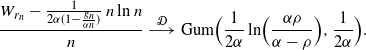 \begin{align*}&\frac{W_{r_n} - \frac {1} {2\alpha(1 - \frac {g_n} {\alpha n})}\, n \ln n}{n}\ {\buildrel {\mathcal{D}} \over \longrightarrow} \ {\rm Gum} \Bigr (\frac 1 {2\alpha}\ln\Bigl(\frac {\alpha\rho} {\alpha-\rho}\Bigr) , \frac {1}{2\alpha}\Bigl). \end{align*}
Interpretation 3.1. The term  $1/(1 - g_n/(\alpha n))$
can be expanded into an infinite series. If
$1/(1 - g_n/(\alpha n))$
can be expanded into an infinite series. If  $g(n) = \Omega(n/({\ln n})^{1/(k-1)})$
but
$g(n) = \Omega(n/({\ln n})^{1/(k-1)})$
but  $g_n = o(n/({\ln n})^{1/k})$
, the series can be stopped after k terms, and the tail can be claimed in an o(n) remainder. But then, this remainder vanishes upon scaling by n. Slutsky’s theorem [Reference Karr7, p. 146] then assures us that we can truncate the series after k terms. For instance,
$g_n = o(n/({\ln n})^{1/k})$
, the series can be stopped after k terms, and the tail can be claimed in an o(n) remainder. But then, this remainder vanishes upon scaling by n. Slutsky’s theorem [Reference Karr7, p. 146] then assures us that we can truncate the series after k terms. For instance,  $j_n$
might be
$j_n$
might be  $\lceil \frac 2 3 n - 2 n^{\frac 5 8} + 3\rceil $
, i.e., we have
$\lceil \frac 2 3 n - 2 n^{\frac 5 8} + 3\rceil $
, i.e., we have  $g_n =2 n^{\frac 5 8} + O(1)$
, and
$g_n =2 n^{\frac 5 8} + O(1)$
, and  $r_n \sim \frac 3 7 n$
, in which case the theorem takes the simple form
$r_n \sim \frac 3 7 n$
, in which case the theorem takes the simple form
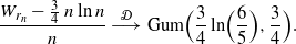 \begin{equation*}\frac{W_{r_n} - \frac 3 4\, n \ln n}{n} \ {\buildrel {\mathcal{D}} \over \longrightarrow} \ {\rm Gum} \Bigr (\frac 3 4\ln\Bigl(\frac {6} {5}\Bigr), \frac 3 4\Bigl). \end{equation*}
Or,  $j_n$
might be
$j_n$
might be  $\lfloor \frac 3 4 n+ 5 n\ln^{-\frac 3 4} n -n\ln^{-\frac 7 9} n + 2 \sqrt[6] n + 19 \ln n - \ln \ln n + 13\rfloor$
, and
$\lfloor \frac 3 4 n+ 5 n\ln^{-\frac 3 4} n -n\ln^{-\frac 7 9} n + 2 \sqrt[6] n + 19 \ln n - \ln \ln n + 13\rfloor$
, and  $r_n \sim \frac 3 5 n $
, in which case we need two terms from the series. The theorem takes the form
$r_n \sim \frac 3 5 n $
, in which case we need two terms from the series. The theorem takes the form
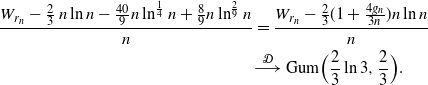 \begin{align*}\frac{W_{r_n} - \frac 2 3\, n \ln n - \frac {40} 9 n\ln^{\frac 1 4} n + \frac 8 9 n\ln^{\frac 2 9} n }{n} &= \frac{W_{r_n} - \frac 2 3 (1 + \frac {4g_n} {3n}) n \ln n}{n} \\ &{\buildrel {\mathcal{D}} \over \longrightarrow} \ {\rm Gum} \Bigr (\frac 2 3\ln 3, \frac 2 3\Bigl). \end{align*}
More generally, If  $g(n) = \Omega(n/({\ln n})^{1/(k-1)})$
but further we have
$g(n) = \Omega(n/({\ln n})^{1/(k-1)})$
but further we have  $g_n = o(n /({\ln n})^{1/k}) )$
, an equivalent form of Theorem 3.1 that captures the infinite number of fine phases is
$g_n = o(n /({\ln n})^{1/k}) )$
, an equivalent form of Theorem 3.1 that captures the infinite number of fine phases is
 \begin{align*}&\frac{W_{r_n} - \frac {1} {2\alpha}\, n \ln n -\frac {1} {2\alpha}\, n \ln n \sum_{i=1}^k (\frac{g_n}{\alpha n})^i }{n} \ {\buildrel {\mathcal{D}} \over \longrightarrow} \ {\rm Gum} \Bigr (\frac 1 {2\alpha}\ln\Bigl(\frac {\alpha\rho} {\alpha-\rho}\Bigr) , \frac {1}{2\alpha}\Bigl). \end{align*}
Remark 3.1. The case  $\rho = \alpha > 0$
presents a degeneracy in Theorem 3.1. An alternative statement to Theorem 3.1 is required.
$\rho = \alpha > 0$
presents a degeneracy in Theorem 3.1. An alternative statement to Theorem 3.1 is required.
Remark 3.2. The Gumbel distribution appears in the waiting time in coupon collection problems, too [Reference Doumas and Papanicolaou3]. For a recent survey of coupon collection problems, see [Reference Ferrante and Saltalamacchia4].
Theorem 3.2. In a community of size n in which one person starts fake news, there are  $j_n-1$
active gullible persons and the remaining persons will never participate in spreading the fake news. Let
$j_n-1$
active gullible persons and the remaining persons will never participate in spreading the fake news. Let  $W_{r_n}$
be the waiting time until
$W_{r_n}$
be the waiting time until  $r_n$
persons have become spreaders. Assume
$r_n$
persons have become spreaders. Assume  $j_n$
and
$j_n$
and  $r_n$
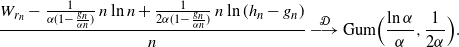
follow (2)–(4). In the case of near depletion, with
$r_n$
follow (2)–(4). In the case of near depletion, with  $\rho = \alpha > 0$
and
$\rho = \alpha > 0$
and  $h_n-g_n \to \infty$
, we have
$h_n-g_n \to \infty$
, we have
 \begin{align*}&\frac{W_{r_n} - \frac {1} {\alpha(1- \frac {g_n} {\alpha n})}\, n \ln n - \frac 1 {\alpha(1- \frac {g_n} {\alpha n})}\, n \ln (h_n - g_n)}{n}\ {\buildrel {\mathcal{D}} \over \longrightarrow} \ {\rm Gum} \Bigr (\frac {\ln \alpha} {\alpha} , \frac {1}{2\alpha}\Bigl).\end{align*}
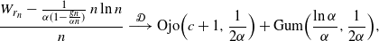
At almost complete depletion, where  $r=j-c$
for integer
$r=j-c$
for integer  $c \ge 0$
, we have
$c \ge 0$
, we have
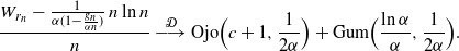 \begin{align*}\frac{W_{r_n} - \frac 1 {\alpha(1- \frac {g_n} {\alpha n})}\, n \ln n }{n} &\ {\buildrel {\mathcal{D}} \over \longrightarrow} \ {\rm Ojo} \Bigr (c+1, \frac {1}{2\alpha}\Bigl)\, +\, {\rm Gum}\Bigl(\frac {\ln \alpha} {\alpha} ,\frac {1}{2\alpha} \Bigr).\end{align*}
The Ojo and Gumbel random variables are independent.
The rest of this manuscript is organized as follows. In Section 4 we set up the waiting time as a convolution of geometric random variables. The convolution is used in a straightforward way in Section 5 to derive the mean and variance of the waiting time, both exactly and asymptotically. After the initial setup of the moment-generating function in Section 6, the asymptotics for the cases far from depletion, near depletion, and for almost complete depletion are separated in Subsections 6.1 and 6.2. The arguments in these subsections constitute proofs for Theorems 3.1 and 3.2. For æsthetic reasons, the case of complete depletion is treated separately in Subsection 6.3.
4. Waiting time
A Markov chain underlies the model. The status of the population can be specified by k, the number of spreaders. When the number of spreaders is k, there are  $j-k$
gullible persons who have not yet heard the fake news, and as stated the number of persons uninterested in participating remains the same throughout. So, it is sufficient to label the state representing the condition of the population at this point with k. The initial state is 1.
$j-k$
gullible persons who have not yet heard the fake news, and as stated the number of persons uninterested in participating remains the same throughout. So, it is sufficient to label the state representing the condition of the population at this point with k. The initial state is 1.
The Markov chain advances from state k to state  $k+1$
with probability
$k+1$
with probability  $p_{n,j,k} = k(\kern1.3pt j-k)/{\binom{n}{2}}$
, and stays at state k with the probability
$p_{n,j,k} = k(\kern1.3pt j-k)/{\binom{n}{2}}$
, and stays at state k with the probability  $1-p_{n,j,k}$
. Thus, it takes a Geo
$1-p_{n,j,k}$
. Thus, it takes a Geo $(p_{n,j,k})$
amount of time to advance from state k to state
$(p_{n,j,k})$
amount of time to advance from state k to state  $k+1$
. The geometric random variables associated with the various states are independent. The waiting time until r persons are spreaders has a representation as a convolution of geometric random variables:
$k+1$
. The geometric random variables associated with the various states are independent. The waiting time until r persons are spreaders has a representation as a convolution of geometric random variables:
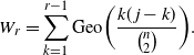 \begin{equation*}W_r = \sum_{k=1}^{r-1} {\rm Geo} \biggl(\frac {k(\kern1.3pt j-k)} {\binom{n}{2}}\biggr).\end{equation*}
5. Average and variance of waiting time
From the geometric convolution set up in Section 4, we find the following.
Proposition 5.1. We have the average
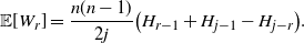 \begin{equation*}{\mathbb E}[W_r] = \frac {n(n-1)}{2j} \bigl(H_{r-1} + H_{j-1} - H_{j-r}\bigr).\end{equation*}
As  $n\to\infty$
, we have
$n\to\infty$
, we have
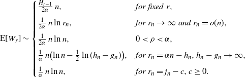 \begin{align*}{\mathrm E}[W_r] \sim\begin{cases} \frac{H_{r-1}} {2\alpha}\, n, & for\ fixed\ r,\\[5pt]
\frac 1 {2\alpha}\, n\ln r_n, & for\ r_n \to\infty\ and\ r_n = o(n),\\[5pt]
\frac 1 {2\alpha}\, n\ln n, &0 < \rho < \alpha,\\[5pt]
\frac 1 {\alpha} \, n\bigl(\ln n - \frac 1 2\ln(h_n-g_n)\bigr), & for\ r_n = \alpha n - h_n, h_n-g_n \to\infty,\\[5pt]
\frac 1 {\alpha} \, n\ln n,& for\ r_n = j_n -c, c \ge 0.\end{cases}\end{align*}
\begin{align*}{\mathrm E}[W_r] \sim\begin{cases} \frac{H_{r-1}} {2\alpha}\, n, & for\ fixed\ r,\\[5pt]
\frac 1 {2\alpha}\, n\ln r_n, & for\ r_n \to\infty\ and\ r_n = o(n),\\[5pt]
\frac 1 {2\alpha}\, n\ln n, &0 < \rho < \alpha,\\[5pt]
\frac 1 {\alpha} \, n\bigl(\ln n - \frac 1 2\ln(h_n-g_n)\bigr), & for\ r_n = \alpha n - h_n, h_n-g_n \to\infty,\\[5pt]
\frac 1 {\alpha} \, n\ln n,& for\ r_n = j_n -c, c \ge 0.\end{cases}\end{align*}
Proof. The expected value of  ${\rm Geo}(p)$
is
${\rm Geo}(p)$
is  $1/p$
, from which we find
$1/p$
, from which we find
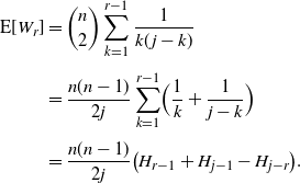 \begin{align*}{\mathrm E}[W_r] &= {\binom{n}{2}}\sum_{k=1}^{r-1} \frac 1 {k(\kern1.3pt j-k)}\\[3pt]
&= \frac {n(n-1)}{2j}\sum_{k=1}^{r-1} \Bigl(\frac 1 {k} + \frac 1 {j-k}\Bigr) \\[3pt]
&= \frac {n(n-1)}{2j} \bigl(H_{r-1} + H_{j-1} - H_{j-r}\bigr).\end{align*}
\begin{align*}{\mathrm E}[W_r] &= {\binom{n}{2}}\sum_{k=1}^{r-1} \frac 1 {k(\kern1.3pt j-k)}\\[3pt]
&= \frac {n(n-1)}{2j}\sum_{k=1}^{r-1} \Bigl(\frac 1 {k} + \frac 1 {j-k}\Bigr) \\[3pt]
&= \frac {n(n-1)}{2j} \bigl(H_{r-1} + H_{j-1} - H_{j-r}\bigr).\end{align*}
Using the asymptotic equivalent in (1), we get the stated asymptotics. □
Remark 5.1. The asymptotic equivalent of the average at  $r_n = j_n - c$
is twice that at
$r_n = j_n - c$
is twice that at  $r_n\sim\rho n$
, for
$r_n\sim\rho n$
, for  $\rho \in (0,\alpha)$
. The mathematical reason for this phase transition is that, for
$\rho \in (0,\alpha)$
. The mathematical reason for this phase transition is that, for  $0< \rho < \alpha$
, each of the three harmonic numbers provides an asymptotic value of
$0< \rho < \alpha$
, each of the three harmonic numbers provides an asymptotic value of  $\ln n$
. That is,
$\ln n$
. That is,  $\ln n$
appears twice positively and once negatively. When
$\ln n$
appears twice positively and once negatively. When  $r_n = j_n - c$
, the negative harmonic number is attenuated to O(1). Thus,
$r_n = j_n - c$
, the negative harmonic number is attenuated to O(1). Thus,  $\ln n$
appears only twice positively. Note how the function
$\ln n$
appears only twice positively. Note how the function  $\ln(h_n-g_n)$
fills the gap at the seam line between the cases
$\ln(h_n-g_n)$
fills the gap at the seam line between the cases  $\rho<\alpha$
and the almost near completion, where
$\rho<\alpha$
and the almost near completion, where  $r_n = j_n - c$
. This explains how the doubling of the average waiting time is not abrupt.
$r_n = j_n - c$
. This explains how the doubling of the average waiting time is not abrupt.
Remark 5.2. Of less interest is the case where  $j_n = o(n)$
. In this case,
$j_n = o(n)$
. In this case,  ${\mathrm E}[W_{r_n}]= O(\kern1.3pt j_n^{-1}n^2\ln j_n)$
.
${\mathrm E}[W_{r_n}]= O(\kern1.3pt j_n^{-1}n^2\ln j_n)$
.
As in the mean of  $W_r$
, the variance of the waiting time exhibits phase transitions. The variance of
$W_r$
, the variance of the waiting time exhibits phase transitions. The variance of  ${\rm Geo} (p)$
is
${\rm Geo} (p)$
is  $(1-p)/p^2$
. Whence, by the independence of the geometric random variables, we have
$(1-p)/p^2$
. Whence, by the independence of the geometric random variables, we have
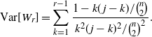 \begin{equation*}{{\mathrm V}{\rm ar}}[W_r] = \sum_{k=1}^{r-1} \frac {1- k(\kern1.3pt j-k)/{\binom{n}{2}}} {k^2(\kern1.3pt j-k)^2/{\binom{n}{2}}^2}.\end{equation*}
After a somewhat tedious expansion of the summand into partial fractions, and summing each individual fraction as a harmonic number, we get the following.
Proposition 5.2. We have the variance
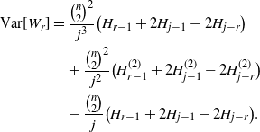 \begin{align*}{{\mathrm V}{\rm ar}}[W_r] &= \frac {{\binom{n}{2}}^2} {j^3} \bigl(H_{r-1} +2 H_{j-1} - 2 H_{j-r} \bigr)\\ &\quad {} + \frac {{\binom{n}{2}}^2} {j^2} \bigl(H_{r-1}^{(2)} +2 H_{j-1}^{(2)} - 2 H_{j-r}^{(2)} \bigr)\\ &\quad {} - \frac {{\binom{n}{2}}} {j} \bigl(H_{r-1} +2 H_{j-1} - 2 H_{j-r} \bigr).\end{align*}
Upon scaling, we have the limits
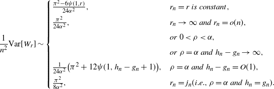 \begin{align*}\frac 1 {n^2} {{\mathrm V}{\rm ar}}[W_r] &\sim\begin{cases} \frac {\pi^2 -6 \psi(1,r)} {24\alpha^2}, &r_n = r \ is\ constant,\\[4pt]
\frac {\pi^2} {24\alpha^2}, & r_n \to \infty\ and\ r_n = o(n),\\[4pt]
& or\ 0< \rho < \alpha,\\[4pt]
& or\ \rho = \alpha\ and\ h_n - g_n \to \infty,\\[4pt]
\frac {1} {24\alpha^2} \big(\pi^2 +12 \psi(1, h_n - g_n+1)\big), & \rho = \alpha\ and\ h_n - g_n = O(1), \\[4pt]
\frac{\pi^2} {8\alpha^2}, & r_n = j_n (i.e.,\rho= \alpha\ and\ h_n = g_n). \end{cases}\end{align*}
\begin{align*}\frac 1 {n^2} {{\mathrm V}{\rm ar}}[W_r] &\sim\begin{cases} \frac {\pi^2 -6 \psi(1,r)} {24\alpha^2}, &r_n = r \ is\ constant,\\[4pt]
\frac {\pi^2} {24\alpha^2}, & r_n \to \infty\ and\ r_n = o(n),\\[4pt]
& or\ 0< \rho < \alpha,\\[4pt]
& or\ \rho = \alpha\ and\ h_n - g_n \to \infty,\\[4pt]
\frac {1} {24\alpha^2} \big(\pi^2 +12 \psi(1, h_n - g_n+1)\big), & \rho = \alpha\ and\ h_n - g_n = O(1), \\[4pt]
\frac{\pi^2} {8\alpha^2}, & r_n = j_n (i.e.,\rho= \alpha\ and\ h_n = g_n). \end{cases}\end{align*}
where  $\psi(1,r+1)$
is the series given in Section 2.
$\psi(1,r+1)$
is the series given in Section 2.
Proof. The steps leading to the exact variance were discussed before the statement of the theorem. Toward asymptotics, observe that all the terms involving first-order harmonics are only  $O(n\ln n)$
, whereas the second-order harmonics have the expansion
$O(n\ln n)$
, whereas the second-order harmonics have the expansion
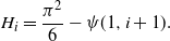 \begin{equation*}H_i = \frac {\pi^2} 6 - \psi(1, i+1).\end{equation*}
Furthermore, the function  $\psi(1, i+1)$
vanishes as
$\psi(1, i+1)$
vanishes as  $i\to\infty$
. □
$i\to\infty$
. □
Remark 5.3. As in the mean, and for a similar reason, the asymptotic equivalent of the variance at  $0 < \rho < \alpha $
is twice that near depletion, where
$0 < \rho < \alpha $
is twice that near depletion, where  $ \rho = \alpha$
.
$ \rho = \alpha$
.
For fixed r, the function  $\psi(1,r+1) = \sum_{s=1}^\infty1/(s+r+1)^2$
lowers the variance below that in the middle range
$\psi(1,r+1) = \sum_{s=1}^\infty1/(s+r+1)^2$
lowers the variance below that in the middle range  $0<\rho<\alpha $
. When r approaches infinity, the
$0<\rho<\alpha $
. When r approaches infinity, the  $\psi$
function begins to vanish, and the case merges into the middle range.
$\psi$
function begins to vanish, and the case merges into the middle range.
Remark 5.4. Barring the case of fixed r, the standard deviation in each of the other phases is of smaller order than the mean of the same phase. Therefore, we have a concentration law following from the Chebyshev inequality. Namely, we have  $W_{r_n} / {\mathrm E}[W_{r_n}] \to 1$
as
$W_{r_n} / {\mathrm E}[W_{r_n}] \to 1$
as  $n\to\infty$
.
$n\to\infty$
.
6. Limit distributions
The geometric random variable  ${\rm Geo}(p)$
has moment-generating function
${\rm Geo}(p)$
has moment-generating function  $p{\rm e}^t/(1-\break (1-p){\rm e}^t)$
, so the convolution in
$p{\rm e}^t/(1-\break (1-p){\rm e}^t)$
, so the convolution in  $W_r$
has the moment-generating function
$W_r$
has the moment-generating function
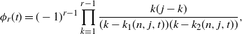
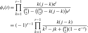 \begin{align}\phi_{r}(t) &= \prod_{k=1}^{r-1} \frac {k(\kern1.3pt j-k){\rm e}^t} {{\binom{n}{2}} - \bigl({\binom{n}{2}} - k(\kern1.3pt j-k) \bigr) e^t} \nonumber \\ &= (-1)^{r-1} \prod_{k=1}^{r-1} \frac {k(\kern1.3pt j-k)} {k^2 - j k + {\binom{n}{2}} (1 - {\rm e}^{-t})}.\end{align}
The asymptotic analysis of this moment-generating function is different for the near-depletion case  $r = j-x_n$
, with
$r = j-x_n$
, with  $x_n \to \infty$
while
$x_n \to \infty$
while  $x_n = o(n)$
, from the asymptotics of the cases that are far away from depletion. Yet again, the case
$x_n = o(n)$
, from the asymptotics of the cases that are far away from depletion. Yet again, the case  $r = j-c$
of near-complete depletion, that is
$r = j-c$
of near-complete depletion, that is  $x_n = O(1)$
, presents another phase change from the case of near depletion.
$x_n = O(1)$
, presents another phase change from the case of near depletion.
An effective way to deal with the representation (5) is to think of the denominator of each term of the product as a factored quadratic function of k. From this vantage point, we see that
 \begin{equation*}\phi_{r}(t) = (-1)^{r-1}\prod_{k=1}^{r-1} \frac {k(\kern1.3pt j-k)} {(k - k_1(n,j,t)) (k - k_2(n,j,t))} ,\end{equation*}
where  $k_1(n,j,t)$
and
$k_1(n,j,t)$
and  $k_2(n,j,t)$
are the roots of the equation
$k_2(n,j,t)$
are the roots of the equation
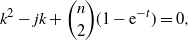 \begin{equation*}k^2 - j k + {\binom{n}{2}}(1-{\rm e}^{-t}) = 0,\end{equation*}
that is, we have the roots
 \begin{equation*}k_i(n,j,t) = \frac 1 2 j \pm\frac 1 2\sqrt{j^2 - 2n(n-1) (1- {\rm e}^{-t})},\quad \mbox{for } i=1,2.\end{equation*}
(We take  $k_1$
to be the root with the positive sign.) We can express the moment-generating function in terms of gamma functions:
$k_1$
to be the root with the positive sign.) We can express the moment-generating function in terms of gamma functions:
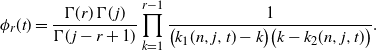 \begin{equation*}\phi_r(t) = \frac{\Gamma (r) \, \Gamma(\kern1.3pt j)} {\Gamma(\kern1.3pt j-r+1)} \prod_{k=1}^{r-1} \frac 1 {\bigl(k_1(n,j,t)-k\bigr) \bigl (k - k_2(n,j,t)\bigr)}.\end{equation*}
We first develop an asymptotic equivalent for  ${\mathrm E}[{\rm e}^{W_r u/n}]$
. When t is small enough (as intended in the use of
${\mathrm E}[{\rm e}^{W_r u/n}]$
. When t is small enough (as intended in the use of  $t=u/n$
, for fixed u and large n), we can work with accurate approximations of the roots. We have
$t=u/n$
, for fixed u and large n), we can work with accurate approximations of the roots. We have
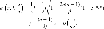 \begin{align*}k_1\Bigl(n,j,\frac u n\Bigr) &= \frac 1 2j+ \frac 1 2j\sqrt{1- \frac {2n(n-1)}{j^2} (1- {\rm e}^{-u/n})} \\ &= j - \frac {(n-1)}{2j}\, u + O\Bigl(\frac 1 n\Bigr). \end{align*}
We are considering  $j=\alpha n - g_n$
, with
$j=\alpha n - g_n$
, with  $\alpha>0$
and
$\alpha>0$
and  $ g_n= o(n)$
, in which case we get
$ g_n= o(n)$
, in which case we get
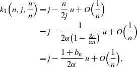 \begin{align}k_1\Bigl(n,j,\frac u n\Bigr) &= j - \frac n {2j}\, u + O\Bigl(\frac 1 n\Bigr) \nonumber\\
&= j - \frac 1 {2\alpha\bigl (1- \frac {g_n}{\alpha n}\bigr)}\, u + O\Bigl(\frac 1 n\Bigr) \nonumber\\[3pt]
&= j - \frac {1+b_n} {2\alpha}\, u + O\Bigl(\frac 1 n\Bigr),\end{align}
\begin{align}k_1\Bigl(n,j,\frac u n\Bigr) &= j - \frac n {2j}\, u + O\Bigl(\frac 1 n\Bigr) \nonumber\\
&= j - \frac 1 {2\alpha\bigl (1- \frac {g_n}{\alpha n}\bigr)}\, u + O\Bigl(\frac 1 n\Bigr) \nonumber\\[3pt]
&= j - \frac {1+b_n} {2\alpha}\, u + O\Bigl(\frac 1 n\Bigr),\end{align}
where  $b_n = \sum_{i=1}^\infty (g_n/(\alpha n))^i$
. Note that
$b_n = \sum_{i=1}^\infty (g_n/(\alpha n))^i$
. Note that  $b_n = O(g_n/n) \to 0$
as
$b_n = O(g_n/n) \to 0$
as  $n\to\infty$
. Similarly, we have
$n\to\infty$
. Similarly, we have
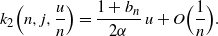 \begin{equation}k_2 \Bigl(n,j,\frac u n\Bigr) = \frac {1+ b_n} {2\alpha}\, u + O\Bigl(\frac 1 n\Bigr).\end{equation}
6.1. Far away from depletion
Consider the case where  $r_n \sim \rho n $
, with
$r_n \sim \rho n $
, with  $0<\rho < \alpha$
. So, there is still a linear number of active gullible persons and their conversion to spreaders will continue for a while. Thus, the case is far away from depleting the pool of active gullible persons.
$0<\rho < \alpha$
. So, there is still a linear number of active gullible persons and their conversion to spreaders will continue for a while. Thus, the case is far away from depleting the pool of active gullible persons.
In this case, we use (6) and (7) to write the asymptotic equivalent:
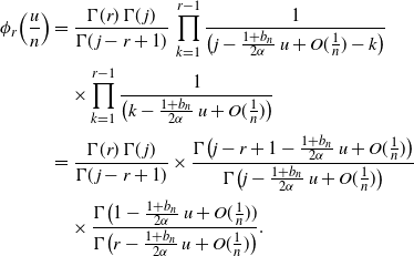 \begin{align*}\phi_{r} \Bigl( \frac u n\Bigr) &= \frac {\Gamma(r)\, \Gamma(\kern1.3pt j) } {\Gamma(\kern1.3pt j-r+1)} \, \prod_{k=1}^{r-1} \frac 1 {\bigl( j - \frac {1+b_n} {2\alpha}\, u + O(\frac 1 n)-k\bigr)}\nonumber\\
& \quad {} \times \prod_{k=1}^{r-1} \frac 1 {\bigl (k - \frac {1+b_n}{2\alpha}\, u + O(\frac 1 n) \bigr)} \nonumber \\[2pt]
&= \frac {\Gamma(r)\, \Gamma(\kern1.3pt j) } {\Gamma(\kern1.3pt j-r+1)} \times \frac {\Gamma \bigl( j - r+1 - \frac {1+b_n} {2\alpha}\, u + O(\frac 1 n) \bigr)} {\Gamma \bigl( j - \frac {1+b_n} {2\alpha}\, u + O(\frac 1 n)\bigr)}\nonumber\\[2pt]
& \quad {} \times \frac {\Gamma\bigl (1 - \frac {1+b_n}{2\alpha}\, u +O(\frac 1 n))} {\Gamma\bigl (r - \frac {1+b_n}{2\alpha}\, u + O(\frac 1 n)\bigr)}. \end{align*}
\begin{align*}\phi_{r} \Bigl( \frac u n\Bigr) &= \frac {\Gamma(r)\, \Gamma(\kern1.3pt j) } {\Gamma(\kern1.3pt j-r+1)} \, \prod_{k=1}^{r-1} \frac 1 {\bigl( j - \frac {1+b_n} {2\alpha}\, u + O(\frac 1 n)-k\bigr)}\nonumber\\
& \quad {} \times \prod_{k=1}^{r-1} \frac 1 {\bigl (k - \frac {1+b_n}{2\alpha}\, u + O(\frac 1 n) \bigr)} \nonumber \\[2pt]
&= \frac {\Gamma(r)\, \Gamma(\kern1.3pt j) } {\Gamma(\kern1.3pt j-r+1)} \times \frac {\Gamma \bigl( j - r+1 - \frac {1+b_n} {2\alpha}\, u + O(\frac 1 n) \bigr)} {\Gamma \bigl( j - \frac {1+b_n} {2\alpha}\, u + O(\frac 1 n)\bigr)}\nonumber\\[2pt]
& \quad {} \times \frac {\Gamma\bigl (1 - \frac {1+b_n}{2\alpha}\, u +O(\frac 1 n))} {\Gamma\bigl (r - \frac {1+b_n}{2\alpha}\, u + O(\frac 1 n)\bigr)}. \end{align*}
The gamma function is continuous on  $\mathbb R^+$
. As
$\mathbb R^+$
. As  $b_n = O(g_n/n)\to 0$
, it follows that
$b_n = O(g_n/n)\to 0$
, it follows that
 \begin{equation*} \Gamma\Bigl(1-\frac {1+b_n}{2\alpha}\, u + O\Bigl(\frac 1 n\Bigr)\Bigr) \to \Gamma\Bigl(1-\frac {1}{2\alpha}\, u \Bigr) \quad\mbox{as } n\to \infty.\end{equation*}
We take the remaining gamma functions in pairs, and to each pair we apply the Stirling approximation of the gamma function. So, we have
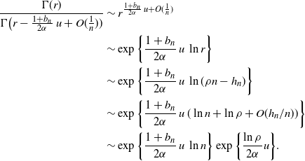 \begin{align} \frac {\Gamma(r)} {\Gamma\bigl (r - \frac {1+b_n}{2\alpha}\, u + O(\frac 1 n))} &\sim r^{\frac {1+b_n}{2\alpha}\, u + O(\frac 1 n)} \nonumber \\ &\sim \exp\bigg\{ \frac {1+b_n}{2\alpha}\, u\, \ln r\bigg\} \nonumber\\ &\sim \exp\bigg\{ \frac {1+b_n}{2\alpha}\, u\, \ln (\rho n - h_n)\bigg\}\nonumber\\ &\sim \exp\bigg\{ \frac {1+b_n}{2\alpha}\, u\, (\ln n + \ln \rho +O(h_n/n))\bigg\}\nonumber\\ &\sim \exp\bigg\{ \frac {1+b_n}{2\alpha}\, u\, \ln n\bigg\} \exp\bigg\{ \frac {\ln \rho}{2\alpha} u\bigg\}.\end{align}
Following similar steps, we find
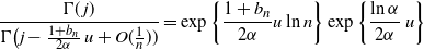 \begin{align} \frac { \Gamma(\kern1.3pt j) } {\Gamma \bigl( j - \frac {1+b_n} {2\alpha}\, u + O(\frac 1 n))} = \exp\bigg\{ \frac {1+b_n}{2\alpha} u \ln n \bigg\} \exp\bigg\{\frac {\ln\alpha} {2\alpha}\, u\bigg\} \end{align}
and
 \begin{equation} \frac {\Gamma \bigl( j - r+1 - \frac {1+ b_n} {2\alpha}\, u + O(\frac 1 n)\bigr) } {\Gamma(\kern1.3pt j-r+1)} \sim \exp\bigg\{-\frac {1+b_n} {2\alpha}\, u\ln n\bigg\} \exp\bigg\{ - \frac {\ln(\alpha-\rho)} {2\alpha}\, u\bigg\}.\end{equation}
The critical term on the right-hand side of each of (8), (9), and (10) is  $\ln n$
. It appears in these equations twice positively and once negatively. Putting these elements together, we can now assert that
$\ln n$
. It appears in these equations twice positively and once negatively. Putting these elements together, we can now assert that
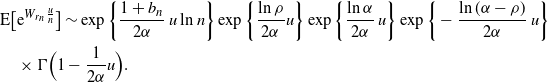 \begin{align*} & {\mathrm E}\bigl[{\rm e}^{W_{r_n} \frac u n}\bigr] \sim \exp\bigg\{\frac {1+b_n}{2\alpha}\, u \ln n\bigg\} \exp\bigg\{\frac {\ln \rho}{2\alpha} u\bigg\} \exp\bigg\{\frac {\ln\alpha} {2\alpha}\, u\bigg\} \exp\bigg\{- \frac {\ln(\alpha-\rho)} {2\alpha}\, u\bigg\} \\ & \quad \times \Gamma\Bigl(1-\frac {1}{2\alpha} u \Bigr).\end{align*}
In other words, we have
 \begin{equation*}{\mathrm E}\biggl[\exp\bigg\{\left(W_{r_n} - \frac {1+b_n} {2\alpha}\, n \ln n\right)\frac u n\bigg\}\biggr] \to \exp\bigg\{\frac u {2\alpha}\ln\left(\frac {\alpha\rho} {\alpha-\rho}\right)\bigg\} \, \Gamma \Bigl(1 - \frac 1 {2\alpha}\, u\Bigr) .\end{equation*}
The right-hand side is the moment-generating function of a Gumbel random variable with location parameter  $(2\alpha)^{-1}\ln (\alpha\rho/(\alpha-\rho))$
and scale parameter
$(2\alpha)^{-1}\ln (\alpha\rho/(\alpha-\rho))$
and scale parameter  $1/(2\alpha)$
. By the Lévy continuity theorem [7, p. 172], convergence of moment-generating functions implies convergence in distribution. In other words, we have
$1/(2\alpha)$
. By the Lévy continuity theorem [7, p. 172], convergence of moment-generating functions implies convergence in distribution. In other words, we have
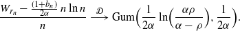 \begin{equation*}\frac{W_{r_n} - \frac {(1+b_n)} {2\alpha}\, n \ln n}{n} \ {\buildrel {\mathcal{D}} \over \longrightarrow} \ {\rm Gum} \Bigr (\frac 1 {2\alpha}\ln\Bigl(\frac {\alpha\rho} {\alpha-\rho}\Bigr) , \frac {1}{2\alpha}\Bigl).\end{equation*}
This completes a proof of Theorem 3.1.
6.2. Near depletion (up to lower-order perturbation)
Suppose  $r_n = \alpha n - h_n$
for perturbation function
$r_n = \alpha n - h_n$
for perturbation function  $h_n$
that is o(n) and
$h_n$
that is o(n) and  $r_n \le j_n$
, so necessarily we have
$r_n \le j_n$
, so necessarily we have  $h_n \ge g_n$
. We have to separate two cases: (a) when
$h_n \ge g_n$
. We have to separate two cases: (a) when  $h_n - g_n \to \infty$
, and (b) when
$h_n - g_n \to \infty$
, and (b) when  $h_n - g_n$
remains bounded.
$h_n - g_n$
remains bounded.
In case (a), the alternative to (10) is then
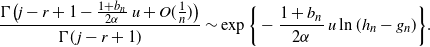 \begin{equation*}\frac {\Gamma \bigl( j - r+1 - \frac {1+ b_n} {2\alpha}\, u + O(\frac 1 n)\bigr) } {\Gamma(\kern1.3pt j-r+1)} \sim \exp\bigg\{-\frac {1+b_n} {2\alpha}\, u\ln (h_n - g_n)\bigg\}.\end{equation*}
Note that the  $\ln n$
terms in (10) are annulled and
$\ln n$
terms in (10) are annulled and  $\ln n$
appears only twice positively in
$\ln n$
appears only twice positively in  $\phi_{r}(t)$
. The alternative statement to Theorem 3.1 is then
$\phi_{r}(t)$
. The alternative statement to Theorem 3.1 is then
 \begin{align*}&\frac{W_{r_n} - \frac {1} {\alpha(1 - \frac {g_n} {\alpha n})}\, n\ln n + \frac {1} {2\alpha(1 - \frac {g_n} {\alpha n})}\, n\ln (h_n-g_n)}{n} \ {\buildrel {\mathcal{D}} \over \longrightarrow} \ {\rm Gum} \Bigr (\frac {\ln \alpha} {\alpha} , \frac {1}{2\alpha}\Bigl). \end{align*}
Remark 6.1. Note how the coefficient of  $n\ln n$
is doubled as compared to the cases that are far away from depletion.
$n\ln n$
is doubled as compared to the cases that are far away from depletion.
In case (b), the Stirling approximation is not applicable to the pair of gamma functions in (10), as the argument of both gamma functions remains bounded. Here we have  $j_n = \alpha n - g_n$
,
$j_n = \alpha n - g_n$
,  $r_n = \alpha n - (g_n + x_n)$
, with
$r_n = \alpha n - (g_n + x_n)$
, with  $x_n = O(1)$
. So, we have
$x_n = O(1)$
. So, we have  $j_n-r_n = x_n$
. There is a large variety in how the term
$j_n-r_n = x_n$
. There is a large variety in how the term  $x_n$
behaves. It might be oscillating, and as we shall see shortly, this does not lead to convergence. We focus on the more interesting case when
$x_n$
behaves. It might be oscillating, and as we shall see shortly, this does not lead to convergence. We focus on the more interesting case when  $x_n = c > 0$
is a constant. So, we have
$x_n = c > 0$
is a constant. So, we have
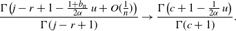 \begin{equation*}\frac {\Gamma \bigl( j - r + 1 - \frac {1+ b_n} {2\alpha}\, u + O(\frac 1 n)\bigr) } {\Gamma(\kern1.3pt j-r+1)} \to \frac {\Gamma \bigl(c+ 1 - \frac {1} {2\alpha}\, u \bigr) } {\Gamma(c+1)} .\end{equation*}
The moment-generating function in this phase is
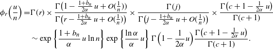 \begin{align*}\phi_{r} \Bigl( \frac u n\Bigr) = & \Gamma(r) \times \frac {\Gamma\bigl (1 - \frac {1+b_n}{2\alpha}\, u + O(\frac 1 n))} {\Gamma\bigl (r - \frac {1+b_n}{2\alpha}\, u + O(\frac 1 n)\bigr)}\times \frac{\Gamma(\kern1.3pt j)} {\Gamma \bigl( j - \frac {1+b_n} {2\alpha}\, u + O(\frac 1 n)\bigr)} {}\times \frac {\Gamma \bigl(c+ 1 - \frac {1} {2\alpha}\, u \bigr) } {\Gamma(c+1)} \\
&\sim \exp\bigg\{\frac {1+b_n}{\alpha}\, u \ln n\bigg\} \exp\bigg\{\frac {\ln\alpha} {\alpha}\, u\bigg\} \, \Gamma\Bigl(1-\frac {1}{2\alpha} u \Bigr) \frac {\Gamma \bigl(c+ 1 - \frac {1} {2\alpha}\, u \bigr) } {\Gamma(c+1)}.\end{align*}
\begin{align*}\phi_{r} \Bigl( \frac u n\Bigr) = & \Gamma(r) \times \frac {\Gamma\bigl (1 - \frac {1+b_n}{2\alpha}\, u + O(\frac 1 n))} {\Gamma\bigl (r - \frac {1+b_n}{2\alpha}\, u + O(\frac 1 n)\bigr)}\times \frac{\Gamma(\kern1.3pt j)} {\Gamma \bigl( j - \frac {1+b_n} {2\alpha}\, u + O(\frac 1 n)\bigr)} {}\times \frac {\Gamma \bigl(c+ 1 - \frac {1} {2\alpha}\, u \bigr) } {\Gamma(c+1)} \\
&\sim \exp\bigg\{\frac {1+b_n}{\alpha}\, u \ln n\bigg\} \exp\bigg\{\frac {\ln\alpha} {\alpha}\, u\bigg\} \, \Gamma\Bigl(1-\frac {1}{2\alpha} u \Bigr) \frac {\Gamma \bigl(c+ 1 - \frac {1} {2\alpha}\, u \bigr) } {\Gamma(c+1)}.\end{align*}
The corresponding limit theorem is
 \begin{equation}\frac{W_{r_n} - \frac {1} {\alpha(1 - \frac {g_n} {\alpha n})}\, n\ln n}{n} \ {\buildrel {\mathcal{D}} \over \longrightarrow} \ {\rm Ojo} \Bigr ( c+1, \frac {1}{2\alpha}\Bigl) \,+\, {\rm Gum}\Bigl( \frac {\ln\alpha} {\alpha},\frac {1}{2\alpha} \Bigr),\end{equation}
and the Ojo and Gumbel random variables in the limit are independent.
6.3. Complete depletion
In the case of complete depletion, when  $r=j$
, the variable
$r=j$
, the variable  $W_j$
represents the waiting time until all the potential spreaders are converted into active spreaders. Attention was drawn to this case in the literature of alternative models. In this case, the generalized Gumbel random variable in (11) comes down to an ordinary Gumbel random variable, leading to the convergence relation
$W_j$
represents the waiting time until all the potential spreaders are converted into active spreaders. Attention was drawn to this case in the literature of alternative models. In this case, the generalized Gumbel random variable in (11) comes down to an ordinary Gumbel random variable, leading to the convergence relation
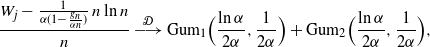 \begin{align*}\frac{W_{j} - \frac {1} {\alpha(1- \frac {g_n} {\alpha n})}\, n\ln n}{n} &\ {\buildrel {\mathcal{D}} \over \longrightarrow} \ {\rm Gum}_1 \Bigr ( \frac {\ln\alpha} {2\alpha}, \frac {1}{2\alpha}\Bigl) \,+\, {\rm Gum}_2\Bigl( \frac {\ln\alpha} {2\alpha},\frac {1}{2\alpha} \Bigr), \end{align*}
and the two Gumbel random variables  $ {\rm Gum}_1$
and
$ {\rm Gum}_1$
and  ${\rm Gum}_2$
are independent. Only for æsthetic reasons (to symmetrize the two Gumbel random variables) do we split the term
${\rm Gum}_2$
are independent. Only for æsthetic reasons (to symmetrize the two Gumbel random variables) do we split the term  ${\rm e}^{\frac u \alpha \ln \alpha}$
in the limiting moment-generating function into two equal parts; one part is subsumed as a location parameter in
${\rm e}^{\frac u \alpha \ln \alpha}$
in the limiting moment-generating function into two equal parts; one part is subsumed as a location parameter in  ${\rm Gum}_1$
, the other is taken as a location parameter in
${\rm Gum}_1$
, the other is taken as a location parameter in  ${\rm Gum}_2$
.
${\rm Gum}_2$
.
Acknowledgements
The author is indebted to Sheldon Ross for insightful discussions.

