


Introduction
Warming of the climate system is unequivocal, as outlined in the latest IPCC Assessment Reports (Parry et al. Reference Parry, Canziani, Palutikof, van der Linden and Hanson2007; IPCC Reference Field, Barros, Dokken, Mach, Mastrandrea, Bilir, Chatterjee, Ebi, Estrada, Genova, Girma, Kissel, Levy, MacCracken, Mastrandrea and White2014) showing that this phenomenon is largely due to the increased atmospheric concentration of greenhouse gases. Both observed data and simulations of future climate conditions indicate that the effect of global warming will be unequally distributed around the globe, with some areas likely to be affected by climate change (CC) much more than others.
The Mediterranean region has been defined as a possible hotspot for the decades to come, by both increasing temperatures and by relatively large changes in the frequency of extreme climatic events, with relevant impacts on agricultural production (Giorgi Reference Giorgi2006; Saadi et al. Reference Saadi, Todorovic, Tanasijevic, Pereira, Pizzigalli and Lionello2015). The rainfall intensity has been shown to be increasing and changes in the distribution of seasonal rainfall have also been recorded (Kharin et al. Reference Kharin, Zwiers, Zhang and Wehner2013; Toreti et al. Reference Toreti, Naveau, Zampieri, Schindler, Scoccimarro, Xoplaki, Dijkstra, Gualdi and Luterbacher2013; Paxian et al. Reference Paxian, Hertig, Seubert, Vogt, Jacobeit and Paeth2014).
Considering the economic and environmental importance of agriculture, it is crucial to assess the effects of future CC on crop yield and adaptation and mitigation strategies for coping with CC (Bindi & Olesen Reference Bindi and Olesen2011). For this purpose, crop simulation models have been widely used (Donatelli et al. Reference Donatelli, Van Ittersum, Bindi and Porter2002) as they allow evaluation of crop vulnerability to CC and optimization of adaptation/mitigation strategies by combining different climate conditions, fertilization regimes, irrigation, soil tillage, etc. (Kimball et al. Reference Kimball, Kobayashi and Bindi2002; Ainsworth & Long Reference Ainsworth and Long2005).
Many crop simulation studies have been carried out on major crops (soft wheat, maize, potato, rice, etc.), but only a few studies have focused on typical Mediterranean crops such as tomato and other vegetables, durum wheat, olive, grapevine, etc. (Bindi et al. Reference Bindi, Fibbi, Gozzini, Orlandini and Miglietta1996; Guereña et al. Reference Guereña, Ruiz-Ramos, Díaz-Ambrona, Conde and Mínguez2001; Giannakopoulos et al. Reference Giannakopoulos, Le Sager, Bindi, Moriondo, Kostopoulou and Goodess2009; Moriondo et al. Reference Moriondo, Bindi, Kundzewicz, Szwed, Chorynski, Matczak, Radziejewski, McEvoy and Wreford2010, Reference Moriondo, Bindi, Fagarazzi, Ferrise and Trombi2011; Ferrise et al. Reference Ferrise, Moriondo and Bindi2011; Ventrella et al. Reference Ventrella, Charfeddine, Moriondo, Rinaldi and Bindi2012a, Reference Ventrella, Charfeddine, Moriondo, Rinaldi and Bindib, Reference Ventrella, Charfeddine, Giglio and Castellinic).
Among crop simulation models used for assessing the impact of CC on agricultural crops, the Decision Support System for Agrotechnology Transfer (DSSAT) model (Jones et al. Reference Jones, Hoogenboom, Porter, Boote, Batchelor, Hunt, Wilkens, Singh, Gijsman and Ritchie2003) has been the most successfully used worldwide over recent years (Alexandrov & Eitzinger Reference Alexandrov and Eitzinger2005; Soltani & Hoogenboom Reference Soltani and Hoogenboom2007; Jin & Zhu Reference Jin and Zhu2008; Dettori et al. Reference Dettori, Cesaraccio, Motroni, Spano and Duce2011).
Globally, crop evapotranspiration (ET) has increased with the expansion of agricultural lands, and irrigated areas in particular (Klein Goldenwijk & Ramankutty Reference Klein Goldenwijk, Ramankutty and Verheye2004). According to Siebert & Döll (Reference Siebert and Döll2010), consumptive blue water (BW) is defined as the amount of crop ET stemming from irrigation; this water is withdrawn from surface or sub-surface water bodies (e.g. streams, reservoirs, etc.). Green water (GW) use is crop ET stemming from rain infiltrated and stored in the soil. So, under irrigation, total crop water use is the sum of blue and GW use and corresponds to the total actual crop ET.
The assessment of GW and BW for a determined cropping system or crop species is a fundamental step in order to define virtual water flows from the area where the crop is cultivated in the region where the crop is processed or consumed, with important consequences on water management policy from global to continental, country, regional, watershed and finally to farm scale. In other words, a very important aspect of the GW/BW approach concerns the planning of a sustainable use of water resources in agriculture, especially for those areas where water represents the most limiting factor, such as the Mediterranean region, and in particular southern Italy.
The water footprint (WFP) is defined as the total volume of freshwater used to produce the goods and services consumed by the individual or community or produced by the business. In agriculture, water use is measured in terms of water volumes consumed (evaporated or incorporated into a product) and/or polluted per unit of time and the WFP is defined as the ratio between ET and crop yield, computed over the cropping period (Hoekstra et al. Reference Hoekstra, Chapagain, Aldaya and Mekonnen2011). The green and blue component in the WFP of a crop is calculated as the green and blue component in crop water use. For those crops that have high ET that can only be met by irrigation due to a scarcity of rainfall during the crop cycle, it may be particularly interesting to also calculate the ‘blue water requirement’ (BWR), defined as the ratio between BW and yield, an indicator estimating irrigation consumption per unit of product. Comparing different areas or agronomic management practices, the lower the BWR values are, the more efficient is the use of irrigation water. In other words, BWR is the inverse of water use efficiency (WUE) with regard to irrigation consumption and could be a useful indicator for water management policy at the distributed scale, allowing identification of the areas where irrigation is more profitable.
Many studies have reported the WFP of different crops such as rice (Chapagain & Hoekstra Reference Chapagain and Hoekstra2011), cotton (Chapagain et al. Reference Chapagain, Hoekstra, Savenije and Gautam2006), tomato (Chapagain & Orr Reference Chapagain and Orr2009), tea and coffee (Chapagain & Hoekstra Reference Chapagain and Hoekstra2007), wheat (Yang et al. Reference Yang, Chen, Luo, Li and Yu2011) and energy crops (Gerbens-Leenes et al. Reference Gerbens-Leenes, Hoekstra and Van Der Meer2009; Dalla Marta et al. Reference Dalla Marta, Mancini, Natali, Orlando and Orlandini2012). Ventrella et al. (Reference Ventrella, Giglio, Charfeddine and Dalla Marta2015) applied the same methodological approach taken in the current paper to the cultivation of winter durum wheat in Southern Italy.
Although the number of research activities related to the assessment of food and non-food crop water footprints is increasing steadily, few of them have addressed the question of how it is affected by climate and soil variability and projected future climatic conditions.
Based on these considerations, the present study aims to evaluate the impact of CC on water use of industrial tomato cultivated in Southern Italy with particular reference to the consumptive use of green and BW and to WFP, all evaluated at the regional scale.
Materials and methods
The study focused on Puglia (Southern Italy), a region of approximately 19 000 km2 and strategically important for agriculture. Industrial tomato (Lycopersicon esculentum L.) is one of the most important vegetable crops cultivated in the region.
The software AEGIS/WIN, a geographic information system (GIS) interface implemented into the model DSSAT v.4·5, was applied in order to simulate the growth and productivity of tomato in the agricultural and irrigated lands of Puglia according to the land use map.
CROPGRO is a crop model in the DSSAT software package and is one of the most physiologically based agronomic models currently available. It simulates the impacts of weather, soil properties, genotype and management options on daily crop phenological development and growth, as well as on the dynamics of soil water and nitrogen. It calculates potential biomass accumulation as the product of radiation use efficiency and intercepted photosynthetically active radiation (PAR). The percentage of incoming PAR intercepted by the canopy is an exponential function of leaf area index. To run CROPGRO, the input including weather, soil, properties, plant characteristics and experimental data is required. The minimum daily weather dataset requirements of the model are solar radiation (MJ/m2d), rainfall (mm) and Tmin and Tmax (°C). In the present study, the Priestley & Taylor (Reference Priestley and Taylor1972) equation to estimate potential ET was used.
The model was previously calibrated and validated in the test area for tomato (cv. PS 1296; Rinaldi et al. Reference Rinaldi, Ventrella and Gagliano2007). The calibration and validation of the model were carried out in the experimental farm of the Council for Agricultural Research and Analysis of Agricultural Economics (CREA) in Foggia, Italy (41°260′N, 15°300′E, 90 m a.s.l.).
Puglia has a typically Mediterranean climate with temperatures that may fall below 0 °C in winter (in the northern part or on hills) and exceed 40 °C in summer. Annual rainfall ranges between 400 and 550 mm, but is concentrated mostly during the winter.
For the 1975–2005 baseline time period, observed daily data (Tmin, Tmax, rainfall and global solar radiation) were extracted for six cells (50 × 50 km2), evenly distributed across the Puglia territory, from the Joint Research Centre (JRC) Monitoring Agricultural ResourceS (MARS) archive (MARS project http://mars.jrc.ec.europa.eu/). For future climate estimates, time slices were centred over the 2030–2059 (+2 °C) and 2070–2099 (+5 °C) time periods, respectively. Daily data were obtained from the HadCM3 experiment for the A2 SRES IPCC (New Reference New and Rosentrater2005).
To overcome the problem of the coarse resolution in the original Hadley Centre Coupled Model, version 3 general circulation model (HadCM3 GCM), a statistical downscaling procedure based on the LARS-WG (Long Ashton Research Station Weather Generator) (Semenov & Barrow Reference Semenov and Barrow1997; Semenov Reference Semenov2007) was adopted for producing synthetic daily weather data representing the +2 °C (A2) and +5 °C (A5) future scenarios. In order to consider the CO2 fertilization effect, three increasing atmospheric concentrations were selected: 360, 550 and 700 ppm for the 1975–2005 period (baseline), A2 and A5, respectively. However, the effect of CO2 on stomatal conductance and therefore on crop transpiration was not considered in the model.
The soil shapefile was drawn from the outputs of the ACLA2 Project (ACLA2 2001). Several GIS procedures were carried out to spatially combine delineations of the same cartographic units, defining 52 cartographic units (UC). The UC map was overlapped with the soil use maps of SIGRIA Projects (SIGRIA-Progetto Casi 3 2002), considering the cartographic units under rainfed cultivation (for winter wheat) and those under irrigated regimes suitable for tomato cultivation. The cartographic units thus achieved were intersected with the MARS climatic cells obtaining 189 polygons, considered as calculation units to run the crop model for winter wheat cultivation (Ventrella et al. Reference Ventrella, Giglio, Charfeddine and Dalla Marta2015) and 150 polygons for tomato simulation as utilized in this study on the AEGIS/WIN-DSSAT platform.
In order to describe the soil hydrological characteristics, several factors were considered: textural classes in the areas of tomato cultivation, soil depth and available water content (AWC, mm) of the shallowest layer of 1 m, calculated as:
 $$AWC = \mathop \sum \limits_{i = 0}^n h_i(FC_i - WP_i)$$
where h (mm), FC and WP are depth, field capacity and wilting point of the n horizons included in the shallowest layer of 1 m of the soils as reported by ACLA2 (2001).
According to Siebert & Döll (Reference Siebert and Döll2010), the consumptive use of GW and BW was obtained from the soil/plant water balance as simulated by DSSAT in two steps, considering two cropping systems in rainfed and irrigated regimes. The first step considered the rainfed condition and the GW was set equal to the actual ET without irrigation (ETcno_irr):
 $$GW = ETc_{no\_irr}$$
The adoption of irrigation was considered in the second simulation, which was equal to the first step but including irrigation. In such cases, the evapotranspiration (ETcirr) came from rain and irrigation and then the following equation can be used to estimate BW:
 $$BW = ETc_{irr} - GW$$
Consequently, the actual ET is the sum of GW and BW.
Scheduled irrigation using a sprinkler method was programmed to operate when 0·80 of the available crop water in the upper 0·5 m of the soil depth is depleted.
In the current paper, the BWR is considered, i.e. the amount of irrigation water, per unit of dry matter yield, required to meet the atmospheric evapotranspirative demand in order to obtain the maximum crop production, considering water as the limiting factor. Blue water requirement is expressed in terms of t/m3 and calculated as:
 $$BWR = \displaystyle{{BW} \over Y}$$
where Y is the dry matter of tomato yield simulated in irrigated condition.
Descriptive statistics were calculated to synthesize the main features of data distribution for GW, BW, yield and BWR. Kolmogorov–Smirnov, Cramer–von Mises and Anderson–Darling procedures were performed in order to compute goodness-of-fit tests for the null hypothesis that the values of the analysis variable are a random sample from the theoretical normal distribution (SAS 2013).
Data of response variables considered in the study were processed by analysis of variance (ANOVA) to test the effects of climate cells, climate scenario (CS) and soils distributed at regional scale.
In order to study the effect of CC on variable distributions, cumulative probability curves were determined for each scenario. Starting from the baseline, the corresponding values for 0·25 and 0·75 quartile were considered to define low, medium and high values as follows:

In other words, the low values were the lowest values of baseline having a probability equal to or less than 0·25; high values were the highest values with 0·25 probability; medium values were the intermediate values, with a probability of 0·5. The second step was to estimate probability levels for the three defined classes that each variable assumes in the two scenario analyses, A2 and A5, for effect of CC.
Results
Weather data, climate scenarios and soil hydrological characteristics
Mean monthly temperatures and rainfall of baseline (1975–2005) and future climate scenarios (A2 and A5) are shown in Fig. 1 for three areas covering the northern, central and southern parts of the Puglia region. The temperature anomalies were forecast to increase from April to August, but were larger for northern Puglia than the other areas: increases of 3 and 6 °C, or more, were forecast here in August under A2 and A5, respectively.

Fig. 1. Climatic trends of Northern, Central and Southern Puglia for monthly rainfall (bars) and mean temperature (lines) by climate scenario.
Conversely, starting from a regional average of 142 mm under the baseline, larger decreases in seasonal rainfall were detected for northern Puglia than in other areas: decreases of 33 and 68 mm, equivalent to about 0·20 and 0·40 of baseline values, under A2 and A5, respectively. Rainfall reduction in the other two areas was projected to be about half the values for northern Puglia.
A higher concentration of fine and very fine soils was detected in the northern area, where they occupy >0·75 of the area of tomato cultivation v. c. 0·25 of loamy soils. The frequency of clay soils in central and southern areas decreases to 0·70 while the loamy soil frequency increases to 0·30 and 0·27 in central and southern areas, respectively. A small proportion of sandy soil (0·03) was also identified in the southern area. In the northern area, greater soil depth, with a median of 115 cm, was detected while the southern area is characterized by higher variability, as indicated by the difference between the first and third quartile (DFTQ) equal to 55 mm. TheAWC of the shallowest layer of 1 m increases by 44% from the southern to the northern area while this variability, in term of DFTQ, decreases from 64 to 34 mm (Table 1).
Table 1. Soil characteristics in the three study areas of Puglia: percentage distribution of the textural classes in the areas of tomato cultivation, main parameters of the statistical distribution of soil depth and available water content (AWC) of the shallowest layer of 1 m: mean, median and quartile at 0·25 and 0·75

a According to Soil Survey Staff (1998).
Figure 2 shows the spatial distribution of AWC in Puglia, with soils characterized by smaller water reservoirs concentrated in southern, central and coastal areas. Haploxeralf, Haploxererts, Calcixererts/Calcixerept and Rhodoxeralf (Soil Survey Staff 1998) are the main soils occupying 0·30, 0·17, 0·17 and 0·08 of the area considered suitable for tomato. Haploxeralf are fine or loamy-fine, deep soils distributed throughout the territory with a greater prevalence in the northern part. Present in the alluvial valleys and terraces in the lower and upper Tavoliere (flat area in northern Puglia), the Haploxererts soils, with a fine or slightly fine texture, are deep and characterized by vertic properties. Calcixererts/Calcixerept soils (loamy-clay, very deep, calcareous with weak drainage) are common in the north and south of Puglia. Finally, the Rhodoxeralfs, or ‘Terre rosse’ (Red Earths) are typical fine soils of central and southern Puglia, displaced on calcarenite; they are soils with a high degree of evolution, shallow, not calcareous and with good drainage (Soil Survey Staff 1998).
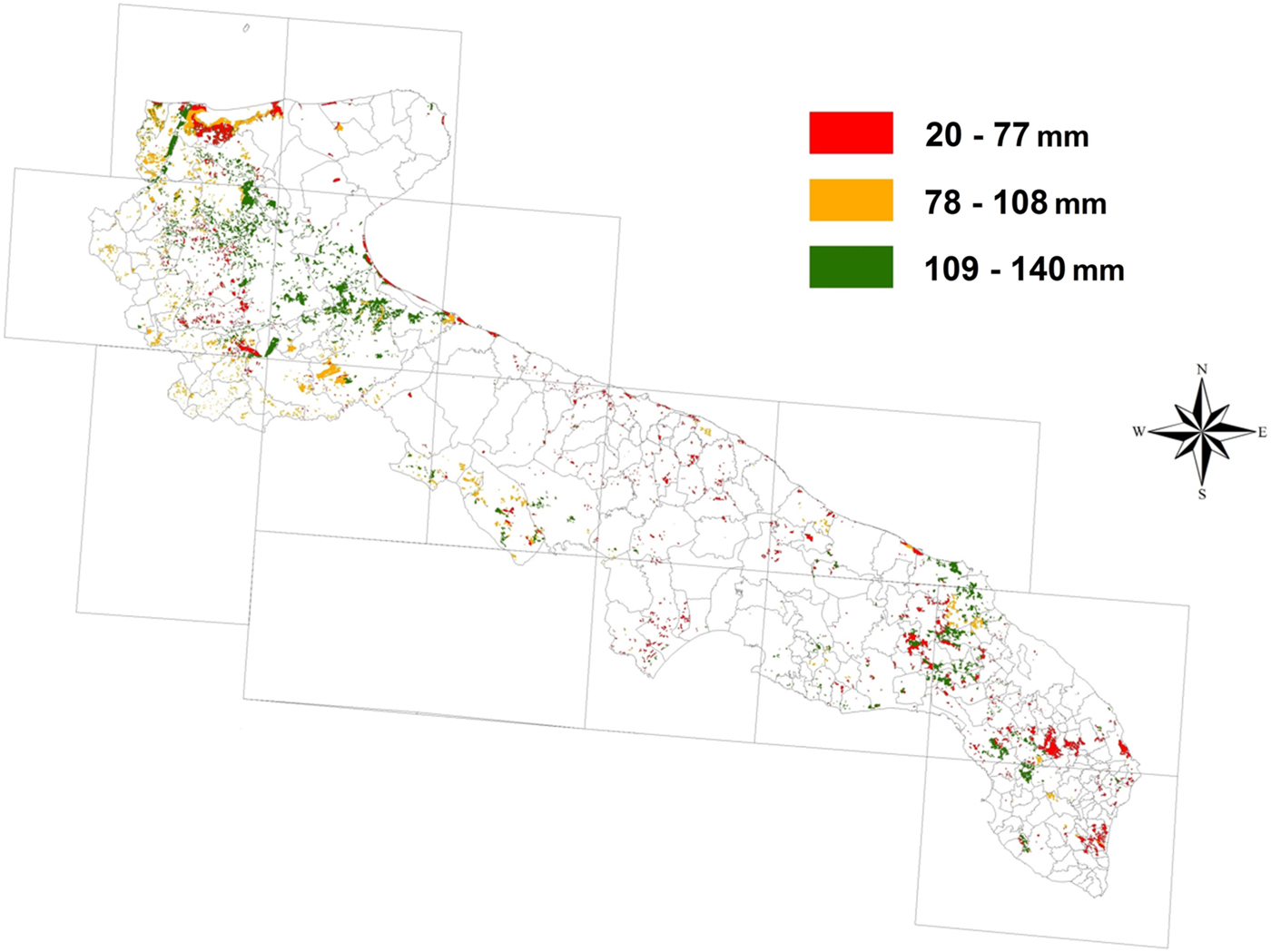
Fig. 2. Distribution map of available water content (AWC, mm) of the shallowest layers of the soils aggregated in three classes of low (red), medium (orange) and high (green) values calculated on the basis of correspondent first and third quartiles.
Statistical distributions of the simulated response parameters
Descriptive statistics for the variables under study and corresponding test results for normal distribution by climatic scenarios are reported in Table 2 and the corresponding curves are shown in Fig. 3. The results for GW indicate a substantial departure from a normal distribution, with positive values of skewness and kurtosis indicating a distribution skewed to the right and heavier tails than for a normal distribution. The departure from normal distribution appears to increase from the baseline to A2 and A5 scenarios, with the median values of future scenarios reduced by 16 and 32% compared with the baseline, respectively. Negative signs of skewness were detected for BW, showing distributions skewed to the left and characterized by median values increasing from 374 mm for a baseline to 406 (+8%) and 440 (+18%) for A2 and A5, respectively. The statistical analysis of Table 2 for tomato yield showed a bimodal distribution (Fig. 3). Such bimodal distribution characterized the three scenarios, with the overall medians of baseline and A2 remaining constant but those for A5 showing a significant decrease of 10% compared with the baseline. Figure 3 shows a lower peak yield corresponding to about 2·4 t/ha for the baseline, increasing in the future scenarios and reaching a value of 5 t/ha for A2. Such lower distribution was related to the sandy soils on several coastal areas of Puglia.

Fig. 3. Empirical statistical distribution of green and blue water (GW and BW: mm), tomato yield (t/ha), blue water requirement (BWR, m3/t) and water footprint (WFP, m3/t) under baseline (BAS), A2 and A5 scenarios.
Table 2. Statistical distribution main parameters by climate scenario: s.d., standard deviation; SKE, Skewness; KURT, kurtosis; Q1, 1st quartile; Q3, 3rd quartile. The Kolmogorov–Smirnov, Cramer–von Mises and Anderson–Darling statistics, with the correspondent P-values of a larger value under the null hypothesis, are also reported

Compared with previous variables, the statistical distribution of BWR and WFP showed very high values of skewness and kurtosis, indicating higher departures from a normal distribution, with distributions highly skewed to the right and heavy tails. The overall median values indicated significant reductions of about 23 and 14% under A5 compared with the baseline for BWR and WFP, respectively. The three tests confirmed significant departures from a normal distribution for all the variables under study and for each scenario analysed.
Figure 4 reports the regional distribution of BW and BWR under the three scenarios. In general, high values of BW and BWR, i.e. larger than the corresponding third quartile and indicated in red colour, were concentrated in the northern part of the region, particularly in coastal areas closed to Gargano's Cape. The distribution patterns of low/high values, both for BW and BWR, detected under the baseline were roughly confirmed under A2 and A5. Moreover, Fig. 4 highlights the variability of BW and BWR due to soil within the same climatic cells.

Fig. 4. Distribution maps of Blue Water (BW) and Blue Water Requirement (BWR) in terms of low (LV), medium (MV) and high (HV) values calculated on the basis of correspondent first and third quartiles. The continuous lines indicate the position of the Northern, Central and Southern areas.
Sources of variability for water consumption, yield and water footprint
For all five response variables considered, the ANOVA results reported in Table 3 showed all the effects of variability sources as highly significant, with ‘Climate scenario’ being the main source of variation followed by ‘Soil’ and ‘Climate cell’. The Soil effect was shown to be the main determinant for yield and WFP with variances equal to 0·60 and 0·50 of that of Climate scenarios, respectively. However, for BW and BWR the effect was about 0·30, while, as expected, it was only 0·20 for GW.
Table 3. Analysis of variance results in terms of Means square for green and blue water (GW and BW), yield, blue water requirement (BWR) and water footprint (WFP). The degrees of freedom (DF) are also reported

The impact of uncertainty due to soil variability is shown in Fig. 5, where the WFP was ordered, by regional area, with increasing values among the soils as determined in the baseline scenario. Parallel lines would show the same ranking among the three scenarios. The ranking among soils, within the regional areas and future climate scenarios, was approximately the same as that of the baseline. However, some soils, i.e. profile P126, P175, P406 and P360, tended to have systematically high values of WFP although with some important departures, such as soil no. 360, which tended to be penalized more (high WFP values) in the baseline than A2 and A5. Soil profiles P126 and P175, Haploxerert and Haploxeralf respectively, are fine soils present in the Tavoliere plain (northern area) with vertic properties (P126) and slow drainage (P175). However, P406 (Xeropsamment) and P360 (Haploxeralf) are localized in the coastal and plain areas of southern Puglia and are deep, fast-draining and highly variable deep soils with good drainage, respectively.

Fig. 5. Water Footprint (WFP) of soils included in three areas of Puglia data-set and sorted in ascending order of baseline scenario. The shaded areas represent ±standard deviations of WFP of soil under the baseline. The blue dashed lines divide the soils into three groups with low, medium and high values of WFP based on baseline ranking and first and third quartile with P < 0·25 and >0·75, respectively.
On the contrary, P026 and P072, Rhodoxeralf and Endopetric, both with good drainage and present in southern Puglia, systematically showed low values of WFP.
Effect of climatic scenarios on statistical distributions
Figure 6 reports the cumulative distribution curve (CDC) for the variables under study (GW, BW, Yield, BWR and WFP) in the three areas that cover the entire Puglia territory (northern, central and southern areas) and under the three scenarios (baseline, A2 and A5). For each graph the probability values of low, medium and high values for A2 and A5 were calculated and are reported for each combination of response variables and area in Table 4. As indicated in the ‘Materials and Methods’ section, the reference values were determined considering the 0·25 and 0·75 quartiles (Q 0·25 and Q 0·75, respectively) of baseline distribution setting ‘low values’ as being ⩽Q 0·25, ‘medium values’ from Q 0·25 and Q 0·75 and ‘high values’ if ⩾Q 0·75. Moreover, the median of the CDC of each curve is reported in Table 5.

Fig. 6. Cumulative statistical distribution (CDC) of green and blue water (GW and BW), blue water requirement (BWR), tomato yield and water footprint (WFP) by area and climate scenario. The vertical lines represent the first and third quartile of the baseline scenario. The probability levels of low, high and medium values under future scenarios and the medians of each CDC are reported in Tables 4 and 5, respectively.
Table 4. Probability levels of low, high and medium values under future scenarios of green and blue water (GW and BW), blue water requirement (BWR), tomato yield and water footprint (WFP) CDC distributions reported in Fig. 6

Table 5. Median values of green and blue water (GW and BW), yield, blue water requirement (BWR) and water footprint (WFP) of CDC distribution reported in Fig. 6, for tomato cultivation in the Puglia region by area and climate scenario

A large reduction in GW is predicted in the northern area with the median dropping from 130 to 100 mm in A2 and to 74 under A5 (reductions of 23 and 43%, respectively). Moreover, the probability of low values increased from 0·25 of baseline to 0·52 and 0·73 under A2 and A5, respectively, while the medium value probabilities drop from 0·5 to 0·4–0·2 and the high values from 0·25 to 0·08 and 0·03 (A2 and A5). This trend was confirmed for the central area although with less extreme values, while probability levels in the southern area were about the same as those of the baseline, where the median values did not show significant departures from an intermediate value of 90 mm. In the southern area, the GW medians were about the same as of those reported for the northern one.
The trend found for BW was opposite to that described for GW, with the northern area characterized by an increase of medians (from 387 to 430 and 490 mm for A2 and A5, respectively) and probability of high values (0·48 and 0·72) and a strong reduction in low value probability (0·13 and 0·09). Such a tendency was confirmed in the other areas, although with less extreme values.
In the northern area, the median yield showed a 20% reduction from baseline to A5 and such a decrease was evident for the highest part of CDC. Moreover, the ‘new’ probability levels have become 0·33, 0·66 and 0·01 for low, medium and high values. The CDC of the central area showed the same behaviour but with less pronounced differences, while in the southern area the yield increased in future scenarios by 19 and 13% under A2 and A5, with a higher probability of achieving medium and high values, compared with the baseline.
As a result of described variations in the previous three variables, the CDC of BWR and WFP were similar for all three areas. For northern and central areas, the composite indicator showed similar CDC under baseline and A2, while major differences were evident for A5. Blue water requirement, as a median parameter, increased under A5, compared with baseline, by 57 and 30%, while WFP increased by 39 and 17%, respectively, for northern and central areas. Under A5 high-value probabilities also increased, to 0·85 and 0·66 for BWR and to about 0·6 for WFP in both the areas.
However, a slight reduction of about 13% was detected for BWR and WFP of the southern area, with low-value probabilities increased up to 0·45 and 0·3 under A5 and A2.
Discussion
Climatic scenarios were shown to be a great influence on all variables in the present study and, in general, future scenarios confirmed the regional distribution pattern of the baseline, a regional pattern that led to the decision to divide the region's territory into three macro-areas in the present study.
Soil was the main determinant for yield, but it also had a significant impact on BW and, to a lesser extent, on GW. This effect is due essentially to retention capacity and therefore susceptibility to drainage losses following intensive rainfall, due to the thickness of the profile and the difference between field capacity and wilting point. In particular, compared with soils with different textures, sandy soils recorded higher BWR and WFP values due to both higher water consumption (in particular BW) and low yields.
Green and blue water
The consumptive use of GW and BW for tomato cultivation in Puglia will be affected by CC; it is closely related to temperature and therefore to the trend of atmospheric evaporative demand. The northern area was characterized by a warmer climate in the baseline scenario and this finding was confirmed in future scenarios, particularly in A5.
In the northern area, with the highest temperatures and lowest rainfall, GW under the baseline was about 130 mm, corresponding to 0·25 of tomato evapotranspiration (ETc) v. the 74 mm under A5 (only 0·13 of Etc). In the other two areas, the contribution of GW to ETc was about 0·17 under A5 and 0·20 for A2.
Therefore, BW tended to increase from southern to northern areas of Puglia and from the baseline to the A5 scenario, confirming this variable, and therefore irrigation practice, as the main limiting factor for obtaining a sustainable yield level of industrial tomato from economic and agronomic points of view.
Yield
In agreement with Ventrella et al. (Reference Ventrella, Charfeddine, Moriondo, Rinaldi and Bindi2012a, Reference Ventrella, Giglio, Charfeddine, Lopez, Castellini, Sollitto, Castrignanò and Fornarob, Reference Ventrella, Charfeddine, Giglio and Castellinic), the findings of the current paper confirmed that CC could negatively affect yields of tomato, a result mainly due to shortening of the crop cycle that particularly affects spring crops such as tomato. Moreover, the results of Ventrella et al. (Reference Ventrella, Charfeddine, Moriondo, Rinaldi and Bindi2012a, Reference Ventrella, Charfeddine, Giglio and Castellinic) highlighted that limiting the global mean temperature change to 2 °C, together with the application of adaptation strategies such as irrigation, nitrogen fertilization, transplanting time optimization or adopting more resilient hybrids, showed a positive effect in minimizing the negative impacts of CC on productivity of tomato cultivated in southern Italy. However, for a global temperature change of 5 °C, environmental conditions were likely to exceed the adaptation capacity of tomato and it was not possible to restore the yield level of the baseline even if the farmer has the possibility of increasing the use of BW to meet the augmented crop water requirements. The latest IPCC reports (Parry et al. Reference Parry, Canziani, Palutikof, van der Linden and Hanson2007; IPCC Reference Field, Barros, Dokken, Mach, Mastrandrea, Bilir, Chatterjee, Ebi, Estrada, Genova, Girma, Kissel, Levy, MacCracken, Mastrandrea and White2014) indicated that +2 °C should be considered a threshold level beyond which the impacts of CC will remain minimal in many areas of the globe for many agricultural crops. Attri & Rathore (Reference Attri and Rathore2003) reported different wheat genotype responses under CC in rainfed and irrigated conditions, while Ferrise et al. (Reference Ferrise, Moriondo and Bindi2011) found that for the entire Mediterranean basin, the projected warmer and drier climate is predicted to increase the risk of yield losses, especially for temperature increases exceeding 2 °C.
Blue water requirement and water footprint
The current paper considered the total WFP and the WFP calculated in terms of BW, i.e. the BWR. The BWR is important because it could support water policies, allowing the concentration of water resources where the efficiency of productivity from irrigation water (i.e. BW) is highest.
As with BW, the value of BWR and WFP also tended to increase moving from the southern to the northern area and from the baseline to the A5 scenario. Blue water requirement and WFP varied similarly in sign and magnitude: in the northern area, they increased under A5 ranging between +40 and +50% compared with baseline, while no significant changes were detected for central and in particular southern area.
Overall medians of BWR and WFP, expressed in term of fresh matter in order to compare the current results with others found in literature, were about 20 and 25 m3/t, respectively, under the baseline and A2. However, the corresponding medians were increased to 25 and 30 m3/t under A5. This is lower than that reported by Mekonnen & Hoekstra (Reference Mekonnen and Hoekstra2011), who showed values of 322 and 171 m3/t for vegetables and tomato, respectively. The average WFP for cereal crops was estimated by Mekonnen & Hoekstra (Reference Mekonnen and Hoekstra2011) at around 1600 m3/t, while for Italian durum wheat Ventrella et al. (Reference Ventrella, Giglio, Charfeddine and Dalla Marta2015) estimated a WFP of >2500 m3/t, simulated in a contest of rainfall regime and baseline scenario due to the lower yields compared with Mekonnen & Hoekstra (Reference Mekonnen and Hoekstra2011). In any case, such values are much higher than those of vegetables, with the main reason being due to differences in crop yields. For fresh tomato cultivated in Spain, Chapagain & Orr (Reference Chapagain and Orr2009) used a mean level yield of 61 t/ha and estimated, for most Spanish regions, a WFP ranging from 60 to 100 m3/t. This large variability present in the literature regarding WFP depends on many factors, influencing such parameters as climate, soil and above all agronomic management, that can determine very high variations in WUE that are the inverse of WFP. This results in a need to define precisely the agronomic context of the cropping system to which the crop WFP data refer. The low values of BWR and WFP in the present study are due to the high simulated yield (about 170 t/ha fresh weight), which can be considered very close to the potential yield because a full irrigation schedule was adopted and no nitrogen stress was applied.
In 2013 and 2014, the average field production of industrial tomato in southern/central Italy was about 80 t/ha (fresh weight), while in a field trial carried out in the province of Foggia (north of Puglia) the yields were almost 130 t/ha, a value similar to the average farm yield (Troccoli et al. Reference Troccoli, De Gregorio, Carrabs, Selvaggio, Olivieri, Demaio, Toriaco, De Sio, Rapacciuolo, Trifirò, Bonaventura and Pecchioni2016).
For industrial tomato, cultivated in Italy, Aldaya & Hoekstra (Reference Aldaya and Hoekstra2010) estimated a national average WFP of 95 m3/t with 60 m3/t coming from blue water (BWR).
Conclusion
The current regional assessment of Green and BW consumption for industrial tomato cultivated in the Puglia region has provided details on crop responses to CC and on how the water resources could be managed in order to optimize crop yield and water productivity. The approach based on estimating the consumptive use of Green and BW and WFP proved to be a useful tool to evaluate the sustainability of tomato cultivation based on irrigated regimes for the agro-pedoclimatic conditions of Puglia. The indicators appeared dependent on CC, spatial and temporal distribution of temperature and rainfall during the crop cycle, but soil hydraulic characteristics, in particular, soil depth, field capacity and wilting point, were also important factors in the diversity of the values.
In this framework, the water indicators were estimated at the regional scale and highly diversified responses were detected within the northern area of Puglia, the most important area for tomato cultivation in the region and also very significant for national production; therefore, it is more vulnerable to CC under the A5 scenario. Such vulnerability, compared with the other two areas of Puglia, was forecast to be in terms of lower consumption of GW and yield and higher BWR and WFP. In particular, for such areas, the current findings confirm that for a global temperature change of 5 °C, environmental conditions are likely to overcome the potential adaptation capacity of tomato cultivation, impacting significantly on crop performance in term of yield and WFP.
The regional distribution patterns of WFP, particularly when calculated in terms of BW consumption, can usefully support the policies of management and planning of water resources.
Future improvement of WFP simulation under CC can be obtained by taking into account the CO2 effect on stomatal conductance and therefore on crop transpiration. Moreover, more realistic estimation of WFP can be obtained through considering and comparing different agronomic strategies, such as deficit v. full irrigation and different levels and type of nitrogen fertilization, a very important agronomic factor strongly interacting with soil water availability in determining yield, yield quality and water use and therefore WFP.
Acknowledgements
The research work described in the present paper was undertaken as a part of COST Action ES1106 ‘Assessment of European Agriculture Water Use and Trade Under Climate Change’ (EURO-AGRIWAT) and ‘Modelling European Agriculture with Climate Change for Food Security’ (MACSUR) knowledge hub within JPI-FACCE (Joint Programming Initiative for Agriculture, Climate Change, and Food Security) and supported Italian Ministry for Agricultural, Food and Forestry Policies (decree n. 24064/7303/15).


