


INTRODUCTION
On dairy and pig farms, animal wastes are a major source of nutrients for crops. However, their application to cropland can result in environmental risks: air, water and soil pollution. Farmers should reduce these risks. Therefore, manure management must take into account the environmental impact of wastes, which encompasses different types of risks. Manure management is closely connected to other aspects of farm management. Reduction of the environmental impact of the wastes can be achieved through different strategic and tactical choices. For instance, the animal feed may be altered in order to reduce nutrient excretion, or waste products may be treated in order to reduce the quantity. Different application methods result in different losses: direct injection of slurry into the soil will reduce ammonia volatilization, for example. Thus, manure management is a generic term including a wide range of decisions. The current study addresses one aspect of the management of agricultural wastes: allocation of the wastes to the fields of the farm to determine which fields, at what rate and when the animal wastes should be applied.
The waste allocation plan is a forecast of the waste applications to be made on every field of the farm during a cultivation year. Since it is made at the beginning of the year, it assumes average climatic conditions. It is a guideline for waste management in the course of the year. Although it may be altered because of variable climatic conditions and labour or machinery constraints, the plan ensures that it is possible to dispose off the wastes using good agronomic and environmental practices. The plan integrates some anticipation into the management of animal wastes, which limits the risks of forced applications due to full storage tanks, or of tank overflows. In some areas, due to environmental regulations, it is mandatory to have a waste allocation plan. This is the case, for example, in the Nitrates Vulnerable Zones (NVZ) in France defined by the European Union's Nitrates Directive (91/676/EC). The allocation plan must be designed for each cultivation year using estimates of the quantities of wastes that will be produced and of the crop needs. In the USA, concentrated animal feeding operations must have a comprehensive nutrient management plan (Centner & Feitshans Reference Centner and Feitshans2006), which comprises several components, including a waste allocation plan.
The development of a waste application plan is a decision taken on the whole-farm scale. The allocation must be made for different fields, different types of wastes and different spreading periods during the year. The fields have different crops and different fertilization histories, and thus different nutritional needs, whereas the wastes have different nutrient contents. The second source of complexity is the diversity of factors that must be taken into account by the decision-maker. The management integrates agronomic rules. For example, some wastes can be applied to some crops, while not to others. Long-term effects like soil-borne diseases or soil organic matter content should also be considered. Moreover, the application plan must take into account the increasingly complex environmental regulations, making it harder for farmers to find suitable solutions. In France, depending upon the region, several regulations may impact waste allocations. The main examples include methods of calculating fertilization rates, distances from waterways and houses within which manure application is prohibited, crop-specific periods during which spreading is banned, banning of spreading during the year following grassland ploughing and mandatory planting of catch crops in winter. The waste allocation plan is based not only on agronomic and environmental rules, but also on many other factors. The constraints on the system, like manure storage capacities, or machinery and labour availability play a key role. Social aspects, like odour problems, may also impact the decision. Economic aspects are also involved, since waste allocations determine the hauling costs of the wastes, and the cost of mineral fertilizers.
However, most modelling studies on waste allocation have assumed farmers to be rational profit maximizers, and restrict the complexity of the decision. Indeed, mathematical programming techniques applied to agricultural decision problems generally aim at improving the decisions taken from an economic and/or environmental point of view. For example, Giasson et al. (Reference Giasson, Bryant and Bills2002) proposed a model of manure allocation to different fields. The model uses a linear programming procedure, which aims at minimizing economic objectives (costs of manure hauling and application, cost of commercial fertilizers) as well as environmental objectives (index of phosphorus pollution risks). The whole-farm model FASSET (Jacobsen et al. Reference Jacobsen, Petersen, Berntsen, Boye, Sørensen, Søgaard and Hansen1998) has a linear programming module which generates management plans for the whole farm, including animal production and crops. Manure allocation is subject to fertilization constraints for each field, as well as labour and machinery constraints. The optimization is based on whole-farm profit. As far as decision support systems (DSSs) are concerned, the Manure Application Planner (MAP) software, described in Schmitt et al. (Reference Schmitt, Levins and Richardson1997), helps farmers design manure application plans. Hence, the software can generate allocations that minimize the costs of manure hauling and application and those of commercial fertilizers, while meeting fertilization constraints for each field. As shown by Edwards-Jones (Reference Edwards-Jones2006), the assumption of perfect rationality has a limited usefulness in the case of decisions subject to factors other than financial ones. The decisions generated can be unrealistic and might not be adopted by farmers.
The current paper presents Fumigene, a model which aims at reproducing the decisions made by farmers for waste allocation plans at the beginning of every cultivation year. The model is intended to be used in a wide range of contexts and is not limited to strategies optimized in terms of economic returns or environmental impact: a wide range of strategies can be simulated. Therefore, the decision is simulated considering a minimum set of constraints and a general strategy, regardless of the motives leading to this strategy. Simulating such a decision process makes it possible to compare waste allocation plans following different strategies. Future applications include coupling Fumigene with environmental evaluation tools, so as to compare the impacts of the strategies tested. A DSS could also be derived. The model is described in the first part of the paper. An evaluation of the capacity of the model to simulate allocations similar to farmer's decisions is presented in the second part. A case study comparing the effect of different phosphorus management strategies on waste allocation is described in the third part.
MODEL DESCRIPTION
Overview
Fumigene translates a management strategy into agricultural waste allocations, i.e. quantities of different wastes to be applied to different fields during two periods of the year, for every simulated year (Fig. 1). It generates waste allocation plans separately for each year. Every year, the allocations generated for the preceding years are used in determining fertilization constraints. The allocations are made by a linear programming procedure, considering field-scale and farm-scale constraints. The objective of the procedure is to select the waste allocation that best suits the farmer's strategy, while meeting constraints at the farm and field scales. The main constraint taken into account at the farm scale is that for each waste, the whole quantity should be applied or exported to another farm. At the field scale, the main constraints taken into account are the practical constraints of application and crop fertilization. For each field, the linear programming procedure considers the maximum quantities of nitrogen (N) and phosphorus (P) that can be applied.

Fig.1. Overview of the model Fumigene.
Fumigene includes a fertilization module which calculates these amounts of N and P so as to match crop requirements based on the yield potential specified by the user. This module needs a fertilization history of each field. When performing simulations for several years, the waste applications generated every year can automatically be included into the fertilization history for the subsequent years, if the actual allocations are not available. The fertilization module can be bypassed if the farmer's fertilization strategy is different from the calculation rules included in the model. In this case, the maximum amounts of N and P for each field are model inputs.
The year is divided into periods in order to take into account the storage capacity constraints. There is usually one critical point at the end of winter. Farmers have to make sure they apply a sufficient quantity in autumn, so as to avoid tank overflows at the end of winter. In Fumigene, in order to represent this constraint adequately, the year is divided into two periods, the first being from August to the start of the winter banned spreading period; the second from the end of the banned period to July. The actual dates of the banned period may vary according to local regulations. The time of application within the broad periods depends on the crop and the waste and can be determined separately. It is not necessary to consider more periods, because it would not impact the allocation.
The waste management strategy is modelled as a set of priorities associated with each field on the one hand and with each (crop, waste, period) triad on the other hand. These priorities are model inputs and mainly reflect agronomic or economic aspects. For example, the fields located far away should be associated with lower priorities, to account for hauling costs. It should be noted that there is no general relationship between distance and priority: 5 km might be acceptable on a farm with widespread cropland, whereas it might be too far on a farm with all fields close to the operation. Variables like mean slope or type of soil should also be taken into account. Furthermore, a farmer might want to maintain the organic matter content of all fields and therefore assign the same priority to each field. Similarly, the waste, crop and period priority values are set according to agronomic rules and are also heavily influenced by the preferences of the decision maker. Because the priorities are set according to the factors considered by the farmer, most management strategies can be represented adequately, even those that are not economically optimal. The approach was chosen in order to be able to simulate the observed variability in agricultural waste management.
The fertilization module
In accordance with the objectives of the model, the fertilization module calculates an estimate of the recommended N and P fertilization rates for each field, assuming average climatic conditions and yields.
Nitrogen
In waste allocation plans, N is the most important, if not the only limiting nutrient considered. It plays a key role in waste allocation. Therefore, the results obtained by the fertilization module are intended to be as close as possible to the calculations made by farmers in France. According to local environmental regulations, the calculation must follow the recommendations of Comité Français d'Etude et de Développement de la Fertilisation Raisonnée (COMIFER). Nitrogen fertilization is calculated using a balance sheet method described in Remy & Hebert (Reference Remy and Hebert1977) and Machet et al. (Reference Machet, Dubrulle, Louis and Scaife1990). Basically, the objective is to predict crop needs and soil supply, considering an average climatic year. Recommended N fertilization is calculated so that supplies match crop requirements. The soil supply includes mineral N content at the beginning of the season and mineralization of organic matter during the year. Several mineralization fluxes are considered, stemming from different organic matter pools. The different terms are:
• mineralization of the soil humus;
• mineralization of the residues of the previous crop;
• mineralization of the residues of the last grassland ploughing;
• mineralization of wastes applied during the previous years (i.e. the effect of fertilization history).
As the method is widely used in France, references are available to estimate the different terms in different contexts, for example in COMIFER (Reference Comifer1996). The method is designed to be readily usable with little data. Mineralization of the wastes of previous years is estimated using a table of reference values depending on average frequency of waste application and type of waste applied. However, different types of waste may have been applied, with an irregular frequency, and the automatic choice of the closest reference value is not trivial. In Fumigene, the fertilization history of each field is available and the calculation of mineralization following a waste application is based on an equation of ‘decay series’ proposed by Pratt et al. (Reference Pratt, Davis and Sharpless1976). This is an exponential equation where the mineralization rate varies for each year after the application. As the parameters proposed for farm yard manure (FYM) were not consistent with recent experiments, the present work uses those of Morvan et al. (Reference Morvan, Ruiz and Viaud2007). All the parameters used for this work are given in Table 1. For a given year y, the effect of the waste applications of previous years is the sum of the N mineralizations as calculated by the decay series. This system requires more data than the original method, but is more flexible in the case of irregular waste applications.
Table 1. Dynamics of the mineralization of the agricultural wastes: the proportions of total N available for crop uptake during the years after application. These parameters were required only for the Derval simulations, and are taken from Pratt et al. (Reference Pratt, Davis and Sharpless1976) and Morvan et al. (Reference Morvan, Ruiz and Viaud2007)

Grasslands may receive N from grazing animals (cows or heifers). The quantity of N excreted on grazed fields is an input to the model and can be estimated according to daily excretion of N and time spent in grazing. For the proportion of N available for crop uptake during the year of excretion, a wide range of values was found in different studies (for example, Deenen & Middelkoop Reference Deenen and Middelkoop1992; Decau et al. Reference Decau, Simon and Jacquet2003). In Fumigene, this proportion was fixed at 0·15, but can be changed by the model user. Thereafter, excretion is treated as applied slurry.
Phosphorus
Concerns over P losses due to waste management are more recent and till recently many farmers did not try to limit excess P due to waste applications. The mode of calculation presented here is a proposition exploring how this could be done, for use in the application of Fumigene comparing different scenarios. Phosphorus is less mobile in soils than N, and it is possible to balance fertilization over several years. It was decided to constrain the running average of the yearly field-scale P balance. Each year and for each field, P balance is calculated as the sum of the P in the fertilizers (mineral and organic) minus P exported by the crop. Phosphorus excreted by grazing animals is added to the P applied during the year. Then, P applied the following year is calculated so that the running average over N years does not exceed a threshold:

The number of years over which the running average is calculated is a parameter of the simulation, which should reflect the average length of the crop rotations. The limit of the running average (Pbalmax) is a model input, specified for each field. This mode of calculation is very flexible on a yearly basis. For example, high P fertilization is allowed if a low fertilization has occurred during the bygone years. However, in the long term, Pbalmax determines a trend in the evolution of the soil P content. Pbalmax should be positive for fields where the P-content is low: positive balances are acceptable. In contrast, Pbalmax should be negative in fields where the P-content is high and thus should be reduced.
When this module is used, the N and P requirements, as calculated above, are passed on to the optimization module.
The optimization module
The optimization module generates the waste allocation schedule for one year, using a mixed integer linear programming method.
Variables
The variables to be optimized represent the quantity of each waste applied to each field or exported during each of the two periods of the year. The quantity of waste w to be applied to field f during period p (in t or m3/ha) is denoted by
The quantity of waste w to export during period p is denoted by
Some auxiliary variables are needed to express some constraints. The Boolean variable indicating whether or not waste w is applied on field f during period p is denoted by
The number of wastes and of fields is denoted respectively as
Farm-level constraints
For each waste, the total quantity to be spread or exported should match the quantity expected to be produced during the year. The quantity is an input of the model. It can be estimated by the user, with the methods commonly used in waste allocation plans, i.e. either considering the average of the quantities produced during the previous years or according to the projected feeding plan and quantities of straw for bedding and to the properties of the waste storage units, assuming an average climatic year if rain is added.
![\hskip-15\eqalign{\tab \forall w \in \left[ {1\comma N_{W} } \right]\colon \cr \tab \sum\limits_{f \equals \setnum{1}}^{N_{F} } {\sum\limits_{p \equals \setnum{1}}^{\setnum{2}} {\left( {X_{w\comma {\kern 1pt} f\comma {\kern 1pt}p} \times {\rm Area}_{f} } \right)} } \plus \sum\limits_{p \equals \setnum{1}}^{\setnum{2}} {E_{w\comma {\kern 1pt}p} } \equals Q_{w} \cr \tab \left\{ \!{\matrix{ {{\rm Area}_{f} } \hfill \tab {{\rm is\ the\ area\ of\ field\ }f{\rm \ where\ \right }}\hfill\cr\tab{{\rm spreading\ is\ allowed}} \hfill \cr {Q_{w} } \hfill \tab {{\rm is\ the\ projected\ total\ quantity\ \right }}\hfill\cr\tab{{\rm of\ waste\ }w} \hfill \cr} } \right. \cr} \hskip-30pt](https://static.cambridge.org/binary/version/id/urn:cambridge.org:id:binary:20170407101600981-0558:S0021859608008034:S0021859608008034_eqn2.gif?pub-status=live)
Capacity to store the wastes is often limited; therefore, it may be necessary to dispose off at least a certain quantity of each waste during each of the two periods. For instance, if the slurry storage capacity is equivalent to 9 months of production, the decision maker may want to spread at least 0·25 of the slurry during the autumn and at least 0·25 during the spring period. Spreading all the slurry in autumn, or in spring, is not a feasible solution.
![\eqalign{\tab \forall w \in \left[ {1\comma N_{W} } \right]\quad {\rm and}\quad \forall p \in \left[ {1\comma 2} \right]\colon \cr \tab \sum\limits_{f \equals \setnum{1}}^{N_{f} } {\left( {X_{w\comma {\kern 1pt}f\comma {\kern 1pt}p} \times {\rm Area}_{f} } \right)} \plus E_{w\comma {\kern 1pt}p} \ges {\rm MinProp}_{w\comma p} \times Q_{w} \cr \tab \left\{\! {\matrix{ {{\rm MinProp}_{w\comma {\kern 1pt}p} } \hfill \tab {{\rm is\ the\ minimum\ proportion\ of\ \right }}\hfill\cr\tab{{\rm waste\ }w{\rm \ that\ should\ be\ \right }}\hfill\cr\tab{{\rm disposed\ off\ during\ period\ }p} \hfill \cr}\hskip-30pt} \right. \cr}](https://static.cambridge.org/binary/version/id/urn:cambridge.org:id:binary:20170407101600981-0558:S0021859608008034:S0021859608008034_eqn3.gif?pub-status=live)
For each waste, the quantity exported can be limited by both a maximum and a minimum. The maximum is the quantity of waste that the cropland can receive. In some cases, the producer may be bound by contract to provide a certain quantity of waste to the receiver. This is why the minimum constraint is included in the model.
![\eqalign{\tab \forall w \in \left[ {1\comma N_{W} } \right]\quad {\rm and}\quad \forall p \in \left[ {1\comma 2} \right]\colon \cr \tab \hskip-32pt\left\{ \!{\matrix{ {E_{w\comma p} \ges {\rm MinExp}_{w\comma p} } \hfill \cr {E_{w\comma p} \les {\rm MaxExp}_{w\comma p} } \hfill \cr} } \right. \cr \tab \hskip-12pt\!\!\!\hskip-15pt\left\{ \!{\matrix{ {{\rm MinExp}_{w\comma p} } \hfill \tab {{\rm is\ the\ minimum\ quantity\ of\ waste }\right } \hfill\cr\tab {w{\rm \ to\ export\ during\ period\ }p} \hfill \cr {{\rm MaxExp}_{w\comma p} } \hfill \tab {{\rm is\ the\ maximum\ quantity\ of\ waste }} \hfill\cr\tab\hskip-28pt w{\rm \ to\ export\ during\ period\ }p} \hfill \cr} } \right. \cr} \hskip-30pt](https://static.cambridge.org/binary/version/id/urn:cambridge.org:id:binary:20170407101600981-0558:S0021859608008034:S0021859608008034_eqn4.gif?pub-status=live)
Field-level constraints
The quantities spread on each field are dependent on the crop needs. The maximum quantities of N and P that can be spread on each field are determined by the fertilization module or specified by the user. Because the quantity and availability of N and P in agricultural wastes are not precisely known, the decision maker may not wish to satisfy the crop needs with organic fertilizers alone. Farmers often choose to keep mineral fertilizers for a part of the crop needs. Therefore, a maximum proportion of the N and P needs can be fixed for the total organic fertilizers (Eqn 5) and for each type of waste (Eqn 6).


The quantities of each waste spread on a field (in tonnes or m3/ha) are limited by practical constraints. Spreaders cannot apply very small quantities and, even if they could, farmers would not do so. Typically, these quantities would be around 15 t/ha for solid wastes, and 20 m3/ha for liquid wastes. In Fumigene, a minimum application rate is specified for each waste. Conversely, very high rates are not possible either, for example because of risks of surface runoff for slurry. A maximum application rate is specified for each waste. The typical values of this parameter are 40 t/ha for solid wastes, and 60 m3/ha for liquid wastes. For some crops, it is possible to make several applications during one period. Thus, the maximum quantity that can be spread during a period is the maximum quantity per application multiplied by the maximum number of applications.

The model does not account for the limitations due to nutrients other than N and P (zinc or copper for example). If a waste has a high content of say copper, Eqn (7) can be used to limit the quantity spread. It is not possible to recalculate this quantity for each field, based on the crop needs and the soil status, as for N and P.
Objective function
The objective function is calculated according to the set of priorities defining the farmer's strategy. A priority value (between 0 and 1) is assigned to each field. This value indicates the degree of acceptability of a waste application on this field. Similarly, a priority value (between 0 and 1) is assigned to each (crop, waste, period) triad. Each year, since the land use is known, it is possible to obtain a priority value for each (field, waste, period) triad by multiplying the field and (crop, waste, period) priorities.

The solution to the linear programming problem should maximize the degree of accordance with this set of priorities, i.e. maximize the priority at which each unit (t or m3) of waste is applied. The objective function is given by the following:
Flexibility
The field-level constraints (Eqns 5–7) should be applied with flexibility, i.e. when no other solution is feasible, it should be possible to apply slightly more waste than is otherwise acceptable. To express this flexibility in mathematical terms, some auxiliary variables were introduced in the model. For each X w, f, p, a variable called: x w, f, pexc is created and represents the ‘excess’ application rate. The flexibility is limited, so as not to obtain extremely high application rates for some fields. The parameter Φtol indicates the tolerance placed on the constraints. For example, Φtol=1·1 means that on each field, the maximum amount of N and P applied (or the maximum application rate of each waste) can be exceeded by 10%.
To do this, Eqns (5)–(7) are duplicated. The new equations are applied to the sum X+X exc (instead of X alone), and the right-hand side terms are modified according to Φtol. The priorities associated with the X exc variables are negative, ensuring that they will be used only if no other solution is feasible.
Implementation
The model was implemented as a stand-alone C++ program. Inputs and outputs are made through standard text files. The resolution of the mixed integer programming problem is made by the library version of the solver ‘lp_solve’ (Berkelaar et al. Reference Berkelaar, Eikland and Notebaert2005). This solver includes a simplex algorithm for the resolution of linear programming problems and a branch-and-bound algorithm for the resolution of integer programming models.
MODEL EVALUATION
The model was applied to two French farms to check whether the incorporation of global management rules into the linear programming problem led to manure allocations consistent with the observed ones. The first case study is the Quintenic school farm, a dairy, beef and pig farm located in Côtes d'Armor. The objective of this application was to test the optimization module in a complex case, with several types of wastes and a high N load. The second case is the Derval farm, an experimental farm managed by the Chambre d'Agriculture Pays de Loire. The objective was to test the model in a simpler situation, but with calculated fertilization rates.
In the rest of the current paper, the years specified for the waste allocation plans are those of harvest. For example, the waste allocation plan for 2006 refers to the plan for the cultivation year 2005/06.
Description of the cases
The Quintenic farm is a dairy, beef and pig farm located in Britanny. It is in an NVZ, thus, since 2002, it is mandatory for the farm managers to design a waste allocation plan every year. The plans made between 2003 and 2006 were collected and used for the evaluation of Fumigene.
The farm produces an average of 270 000 litres milk, 54 young bulls and 2200 pigs (with 100 sows) per year. The total agricultural area of the farm is 70 ha. It comprises 18 ha of grassland, 29 of maize, 17·5 of wheat, 4 of rape and 1·5 of fallow land. Several types of animal wastes are produced on the farm. This includes FYM from dairy cows and sows as well as slurry from pigs, beef and dairy cattle. Because the organic N load on the farm is higher than required, a slurry treatment system was built in 2003. In 2003, half of the pig slurry was treated and since 2005 all the pig slurry is treated. After decantation of the resultant of the treatment, two products can be isolated: sludge and supernatant. These products can be spread on the crops separately, but it is also possible to mix them before application. In this case, the product applied is called treated pig slurry. The model inputs related to the wastes are given in Tables 2 and 3. During the period studied, the management of animal wastes was changed. There was no pig slurry after 2005, it being replaced by a combination of sludge (starting from 2004) and supernatant (starting from 2005).
Table 2. Quantities, N and P contents of the wastes for each simulated year on the Quintenic and Derval farms. The values are taken from the waste allocation plans designed by the farm managers

Table 3. Parameters for the different wastes in the two farms: minimum and maximum application rates, as imposed by machinery constraints, and proportion of total N available for crop uptake during the year of the application

A general waste management strategy was determined during an interview with the person in charge of the crops on the farm. Observation of the waste allocation plans showed that the strategy could be slightly different every year. Furthermore, as mentioned before, the types of waste to be spread change every year. As a result, the strategy used in the simulations was partly determined according to the observed allocation plans.
All fields are close to the farm, and the manager's strategy is to distribute the animal wastes on the whole area (in the long term) in order to maintain the soil organic matter content. Therefore, all fields were considered to have a priority of 1·0. The priorities associated with each (crop, waste, period) triad are given in Table 4. Maize fields are fertilized only with organic N. The entire amount of FYM is applied to maize fields in spring (priority=1·0). Bovine slurry (priority=0·9), treated pig slurry (0·8) or (untreated) pig slurry (0·6) are also applied in spring to complete the N needs of maize. Wheat fields receive all the sludge in autumn (priority=1·0) and some pig slurry (0·9) can be applied in spring. The N needs are then covered by mineral fertilizers, which is beyond the scope of this model. Grasslands may receive any liquid waste: cattle slurry, pig slurry, treated pig slurry or supernatant, either in autumn or spring, with priorities varying between 0·5 and 1·0 (except for treated pig slurry in autumn).
Table 4. Coefficients of priority (between 0 and 1) for each potential waste application in the Quintenic simulations, as established according to the manager's waste management strategy

The storage constraints were taken into account for cattle and pig slurry. For cattle slurry, the constraint imposed was that at least 0·15 be applied during the late summer–autumn period and at least 0·15 during the winter–spring period. As far as pig slurry is concerned, the situation is more complicated because several types of waste are actually in single storage: treated pig slurry, sludge and supernatant. As sludge should mainly be applied on wheat fields in autumn, the minimum proportion applied in autumn was set to 0·80. Conversely, at least half of the treated pig slurry and of the supernatant must be spread in spring. The maximum numbers of applications are given in Table 5.
Table 5. Maximum number of applications of each waste on each crop during each period in the Quintenic simulations, as established by the farm manager

The Derval experimental farm is a dairy farm located in the Pays de Loire region. The waste allocation plans were available for years 2003, 2004 and 2005. The recorded crop rotations on each field since 1995 were also used.
The farm has 80 dairy cows plus 80 heifers and calves. The total farm area is 100 ha, comprising 55 ha of grasslands, 30 ha of maize, 10 ha of wheat and 5 ha of fallow land. Two types of wastes are produced: FYM and slurry; the model inputs describing them can be found in Tables 2 and 3.
FYM is spread preferably on maize fields. The application rate is about 30 t/ha. The maize fields which do not receive FYM are fertilized with 50 m3/ha of slurry. Slurry is also applied on grasslands. On maize, all applications are made during spring, while slurry can be applied to grassland either in autumn (more favourable for poorly drained fields) or in spring/end of winter. This strategy was translated into a set of priorities usable by Fumigene (Table 6). Four fields in permanent grassland are intensely used for grazing. No waste applications are made on these 8·6 ha of fields. The priority of these fields was thus set to 0. There is no particular restriction on the application of wastes to the other fields, whose priorities were set to 1·0. The maximum number of applications was always 1, except for FYM on wheat during period 2 (end of winter–spring), which is impossible.
Table 6. Coefficients of priority (between 0 and 1) for each potential waste application in the Derval simulations, as established according to the manager's waste management strategy

Simulations design
Simulations were performed for each site, using common information for every year wherever possible. In the observed allocation plans, the predicted quantities of waste are different every year, because they depend on the stock variations. Nutrient contents of the wastes are adjusted every year, depending on tests performed during the previous year. Also, in the Quintenic case, the quantities of pig slurry treated increased between 2003 and 2006. Therefore, the quantities and nutrient contents of the agricultural wastes were specified for each year. Every year, some fields can be split into several parts or reunited. Fumigene is not able to represent this kind of management: the fields must be the same every year. The fields used in the simulations were the smallest observed subdivisions during the period. The crops on these fields were those observed.
In the Quintenic case, the waste allocation plans included an N fertilization rate (calculated with the N balance sheet method). This rate was used as the maximum quantity of N to spread on each field. In the Derval case, the N fertilization rate for each field was not known. Hence, these rates were calculated by the fertilization module of Fumigene. This module uses the fertilization history of each field, which was not available. As a result, simulations were performed starting from 1995 onwards, with the observed crop rotations on each field. The results of years 1995–2002 were discarded in the evaluation of Fumigene, since no observed data was available. However, simulating manure allocation for these years made it possible to have a consistent organic fertilization history for each field for years 2003–05.
The fertilization module was parameterized so as to represent the conditions of Derval, using local references and farm records. The quantities of N and P excreted each year on the whole grazing area were taken to be 4284 kg of N and 1147 kg of P2O5 for dairy cows, and 2494 kg of N and 594 kg of P2O5 for heifers. These nutrients were considered to be evenly distributed over the whole grazing area, even though some fields are used only for grazing and others are used for cutting and grazing.
In both the cases, P-related constraints were not used, because the managers did not take them into account directly when allocating organic fertilizers.
Results
Fumigene aims to reproduce manure allocation decisions taken by farmers. In most systems, there are alternative options on a yearly basis. Each year, the model may choose a slightly different solution than the decision maker, yet leading to similar results over a period of several years. For example, consider two maize fields A and B. It is possible, for instance, to spread manure on field A in even years and on field B in odd years, or vice versa. These two solutions are different mathematically, but are equivalent agronomically. Therefore, evaluation of the model is not based on direct comparison of observed and simulated manure allocations for each field and each year. It is based on the degree of accordance of the simulated allocation with the manager's strategy. Comparison of observed and simulated manure allocations is made using several key criteria such as the area of each crop fertilized with each type of waste applied. Furthermore, the results were discussed with the decision-makers, in order to assess the applicability of manure allocations generated by the model and determine the causes of divergence between observed and simulated allocations.
In both the cases, over the periods studied, the decisions generated by the model are in accordance with the strategy used by the manager. Overall, the allocation of wastes to crops is the same in the observed and simulated plans. For each waste, the differences between observed and simulated allocations are small compared to the total quantity. At Quintenic, for each crop, the proportion of the N requirements covered by organic fertilizers is similar in the observed and simulated waste allocations (Fig. 2). Maize is fertilized only with organic fertilizers: it has a high priority for FYM and cattle slurry and thus these wastes are spread on maize until it is saturated. The fertilization level of rape is also correctly simulated, thanks to the seasonal constraints. This analysis could not be performed in the Derval case, since the recommended fertilization rates were not included in the observed waste allocation plans.

Fig. 2. Comparison of nitrogen fertilization through animal wastes in the observed (![]() ) and simulated (
) and simulated (![]() ) waste allocations to nitrogen needs (■), as an average on the whole area of each crop during the four years simulated in the Quintenic case.
) waste allocations to nitrogen needs (■), as an average on the whole area of each crop during the four years simulated in the Quintenic case.
Although the total quantities allocated over the periods studied are correct, some errors appear when analysing the results year by year. For example, at Quintenic (Fig. 3), the application of treated pig slurry to maize was widely over-estimated in 2003 and under-estimated in 2004 and 2005. At Derval (Fig. 4), too much slurry is allocated to grasslands by the model in 2003 and 2004. Conversely, in 2005, too much slurry is applied to maize fields. The quantities misallocated are between 150 and 300 m3, while the total yearly quantity of slurry produced is, on average, 1966 m3.

Fig. 3. Comparison of observed (![]() ) and simulated (
) and simulated (![]() ) quantities of waste allocated to each crop for each year, in the Quintenic case. Quantities are given in tonnes for farm yard manure (FYM), and in m3 for the other wastes.
) quantities of waste allocated to each crop for each year, in the Quintenic case. Quantities are given in tonnes for farm yard manure (FYM), and in m3 for the other wastes.
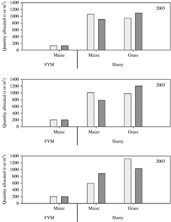
Fig. 4. Comparison of observed (![]() ) and simulated (
) and simulated (![]() ) quantities of waste allocated to each crop for each simulated year, in the Derval case. Quantities are given in tonnes for FYM and in m3 for slurry.
) quantities of waste allocated to each crop for each simulated year, in the Derval case. Quantities are given in tonnes for FYM and in m3 for slurry.
In the model, when an application on one field is decided, the application rate is as high as possible, considering the constraints of the problem. The general behaviour of the model is inherent in linear programming. As a result, the allocation of small quantities, as those observed at Quintenic (Fig. 3), for example, of sludge to maize or of treated pig slurry to wheat, are not correctly simulated. The wastes are applied, as much as possible, on the crop with the highest priority. Even when the total quantity of a waste allocated to a crop is correctly simulated, the area of application and the application rate can be slightly different between the observed and simulated allocations. For example, for sludge applications to wheat at Quintenic (Fig. 5), the average application rate (on fields where an application is made) is higher in the simulated allocation, while the area fertilized is lower. Indeed, one objective of the decision maker is to maintain the organic matter content of all fields. Sludge is distributed evenly between all the wheat fields, while in the simulated allocation some fields do not receive sludge. Interestingly, for FYM applications to maize, the average application rate is lower in the simulated allocation, while the area fertilized is higher. In the observed allocation, the fields with a rotation of crops and grasslands are never fertilized with FYM, but may receive slurry. In the model, all fields are considered to have a specific priority (P f, see Eqn 8) of 1·0, because this value does not depend on the waste. At Derval (Fig. 6), on average during the 3 years, the simulated application rates of slurry to grasslands and FYM to maize are close to the observed ones. Slurry is applied to maize at an application rate of 44 m3/ha in the simulated plan, compared to 50 m3/ha in the observed one. Year by year, the errors are always lower than 15 m3/ha, and seldom exceed 10 m3/ha. The distribution between the two periods of the year was not investigated, as it was not known for all the observed allocation plans.

Fig. 5. Comparison of the areas fertilized (ha/year) in the observed (![]() ) and simulated (
) and simulated (![]() ) waste allocations and of the application rates in the observed (○) and simulated (•) allocations, as averages per waste and crop over the 4 years simulated, in the Quintenic case. Application rates are given in t/ha for FYM and in m3/ha for the other wastes.
) waste allocations and of the application rates in the observed (○) and simulated (•) allocations, as averages per waste and crop over the 4 years simulated, in the Quintenic case. Application rates are given in t/ha for FYM and in m3/ha for the other wastes.

Fig. 6. Comparison of the areas fertilized (ha/year) in the observed (![]() ) and simulated (
) and simulated (![]() ) waste allocations and of the application rates in the observed (○) and simulated (•) allocations, as averages per waste and crop over the 3 years simulated, in the Derval case. Application rates are given in t/ha for FYM and in m3/ha for slurry.
) waste allocations and of the application rates in the observed (○) and simulated (•) allocations, as averages per waste and crop over the 3 years simulated, in the Derval case. Application rates are given in t/ha for FYM and in m3/ha for slurry.
The main causes of error are given in the discussion of the current paper. Globally, the results of the evaluation show that the model can successfully reproduce the decisions taken by farm managers in two very different situations. Fumigene can thus be used in studying the potential impact of a change in strategy or in the constraints.
APPLICATION: IMPACT OF DIFFERENT PHOSPHORUS FERTILIZATION RULES
The model Fumigene was used to study the impact of different P fertilization strategies on the allocation of agricultural wastes. In past decades, soil P content in the western part of France has been rising steadily (Bretagne Environnement 2003). Concerns over the environmental impact of P are growing and a specific regulation might be created. In the current study, P constraints are introduced at the field scale, with two modes of calculation. The potential impact on waste allocation at the farm scale is studied.
Simulations design
The application is based on the Derval case, described in the previous section, and the waste management strategy is the same across the different simulations. Three different rules were tested for the P constraints. In the first simulation (A), the P constraints were not taken into account when allocating agricultural wastes. This simulation is equivalent to the one shown in the evaluation of the model. In the second simulation (B), P fertilization had to be balanced over a 5-year period. Each year, P needs were calculated by the fertilization module of Fumigene, so that the running average of the P balance does not exceed 0 for each field. In a third simulation (C), P fertilization could not exceed the expected P exports of the crop for each planned year. It was permitted to export some wastes to another farm, if no other solution was possible.
Results
The simulations show that integration of P constraints in the decision alters the waste allocations generated (Fig. 7). Considering the P constraints as a running average over 5 years caused small changes in the waste allocation plan. As a total over 3 years, in simulation B, less slurry was applied to maize and grasslands. Instead, it was applied to wheat, which did not receive any waste in simulation A. Balancing P fertilization every year (simulation C) caused bigger changes. More slurry was transferred from grasslands to wheat. FYM could no longer be applied to maize, leaving enough room for slurry applications. Instead, FYM was partly applied to wheat, and the remainder had to be exported. The allocation would be impossible without this option.

Fig. 7. Comparison of the quantities of wastes allocated to each crop for each simulated year, in simulations A (■), B (![]() ) and C (
) and C (![]() ). Phosphorus fertilization is not taken into account in simulation A, and it should be balanced over 5 years in simulation B, or every year in simulation C. Quantities are given in tonnes for FYM and in m3 for slurry.
). Phosphorus fertilization is not taken into account in simulation A, and it should be balanced over 5 years in simulation B, or every year in simulation C. Quantities are given in tonnes for FYM and in m3 for slurry.
The reduction of the total quantities of slurry allocated to maize and grasslands was mainly caused by a reduction in the application rates (Fig. 8). In the case of slurry on grasslands, reduction in the application rate was partly compensated for by an increase in the area fertilized in simulation B, which was not possible in simulation C. The fields grazed by dairy cows can receive low amounts of P. These amounts are lower than the quantity supplied by an application of 25 m3/ha of slurry, which was the minimum allowed. In simulation B, it is possible to apply slurry on these fields to compensate for negative balances during the previous years. This is not permitted in simulation C, so no application is possible on the fields grazed by dairy cows. Therefore, part of the waste had to be exported in this simulation. The absence of FYM applications on maize made it possible to spread slurry on a wider area, but with a lower application rate.

Fig. 8. Comparison of the areas fertilized (ha/year) in simulations A (■), B (![]() ) and C (
) and C (![]() ) and of the application rates in simulations A (•), B (▿) and C (
) and of the application rates in simulations A (•), B (▿) and C (![]() ), as averages per waste and crop over the 3 years simulated. P fertilization is not taken into account in simulation A and it should be balanced over 5 years in simulation B, or every year in simulation C. Application rates are given in t/ha for FYM and in m3/ha for slurry.
), as averages per waste and crop over the 3 years simulated. P fertilization is not taken into account in simulation A and it should be balanced over 5 years in simulation B, or every year in simulation C. Application rates are given in t/ha for FYM and in m3/ha for slurry.
It should be noted that FYM was exported rather than slurry, because FYM has a higher P content. Exporting 1 t of FYM or 1 m3 of slurry, instead of spreading it on maize, impairs equally the objective function of the model, but a given P surplus can be obtained by exporting less FYM than slurry. Hence, the waste allocation in which FYM is exported (rather than slurry) gives a better objective function and is selected by the model. A farmer might prefer to keep applying FYM to maize and transfer more slurry to wheat or to export it.
DISCUSSION
Rationality of the decision maker
Given the complexity of the decision process, the design of waste allocation plans should be modelled using the principle of bounded rationality, which is more in accordance with farmers' decision processes (Attonaty et al. Reference Attonaty, Chatelin and Garcia1999; Edwards-Jones Reference Edwards-Jones2006). Nevertheless, perfect rationality is an assumption often found in decision models using mathematical programming. Models based on economic and/or environmental optimization may generate decisions that are unacceptable to the decision maker. Farmers' strategies may not be optimal in economical terms (Schmitt et al. Reference Schmitt, Levins and Richardson1997) and farmers may base their decisions on factors not included in the models.
The approach presented in the current study focussed on reproducing the decisions taken by a farmer. In Fumigene, the factors taken into account by the decision maker are not explicitly represented. The user generates a set of priorities which reflect the constraints and opportunities of the modelled farm. The strength of the model is its ability to represent a wide range of strategies. On the other hand, Fumigene does not directly propose improved decisions (on a given economic or environmental criterion).
Relevance of the decisions generated
The Quintenic and Derval simulations have shown that the waste allocations generated by the model were similar to the observed ones. Each year, different waste allocations are possible. The objective of the model is not necessarily to make the same decision as the farmer, but to generate a waste allocation that is in accordance with the farmer's strategy. In both the evaluation cases, the allocations made by the model were found to be relevant, in general. Referring to the decision makers, Fumigene generated acceptable decisions in the different situations tested. This showed that the model takes into account the main factors considered when compiling a waste allocation plan. On a year by year basis, differences can arise and several causes of divergence were identified during discussion of the results with the decision makers.
At Quintenic and Derval, the manure allocation plans are designed in winter. The applications made during the preceding autumn are directly integrated, so a part of the specific conditions of the year are known. For example, if limited autumn applications could be made because of bad weather conditions, the manure allocation plan will propose more spring applications. On the other hand, Fumigene is intended to be applied without any knowledge of conditions during the year. Bad weather conditions in autumn are thus not integrated into the model's decision. This explains part of the divergence between the observed and simulated allocations. Furthermore, at Quintenic, the treatment installation was built in 2003. Management of its products had to be devised and the strategy evolved between 2003 and 2006. The objective of the simulations was to have one management strategy applicable for every year. The average strategy does not perfectly suit every year of the transition period observed at Quintenic. The differences between the observed and modelled allocations can be explained by changes in the management strategy. Most farms have stable waste management and this problem does not apply to them.
On the other hand, a few limitations to the model appeared during the simulations. Some elements of the strategies observed could not be represented in the model, like the distribution of one type of waste among different fields with the same crop and similar priorities. This problem is closely connected with the management of organic matter content in soils. Fumigene does not take into account this factor explicitly, whereas farmers may consider it when planning the application of wastes, especially for slow mineralizing wastes like FYM. Different strategies are possible. The decision maker may choose to distribute the waste on the smallest area possible, achieving the whole N needs with the organic fertilizer. On the contrary, another possibility is to distribute the waste evenly over the whole area. The former is easier practically, while the latter is better agronomically and environmentally. Observed strategies are usually a mix of these possibilities. With the linear programming model presented, it is not possible to distribute a waste evenly on the fields for a given crop. In the solution chosen by the model, each application is made at the maximum rate possible, considering the constraints. A possible solution to overcome this limitation would be to assign to each field a priority decreasing with the quantities of wastes applied. However, this would break the linearity of the model and another mathematical programming technique would be required. Distribution of wastes across the area can also be considered over several years. Some types of waste mineralize slowly and it may not be desirable to apply these wastes to the same fields every year. Since Fumigene operates on a yearly basis, reusing information from the past years, this type of decision rule could be included. For example, the application of a waste could cause a reduction in the priority factor of the field, for a given period of time.
Setting only one priority value per field could be viewed as a limitation too, because one might want to have, for each field, one priority associated with each waste or with each season. With a priority value per (field, waste) couple, it would be possible to represent complex cases. For example, a farm with different sites (e.g. a main site for dairy cows and a remote site for heifers) will preferably spread each waste on fields close to its production site. A priority value per (field, period) combination would make it possible to represent cases like Derval better, where the poorly drained fields are preferentially chosen for autumn applications.
Model applications
In the case presented, the objective of balanced P fertilization for each field over 5 years (simulation B) led to a reduction in the waste application rates and to an alteration of the waste allocation plan. Balancing P fertilization for each year (simulation C) led to further reductions in the application rates. Designing a waste application plan was not possible without exporting part of the waste. In a general way, integrating P constraints in manure allocation would not impact all farms the same way. The P/N ratio is generally higher in animal wastes, especially pig slurry, than in plant requirements and it is likely that P constraints would lead to reductions in the application rates compared with those calculated for N alone. As a result, designing a waste application plan would become more complicated, or even impossible, as illustrated by the Derval case. Balancing P fertilization over 5 years seems to be more adapted to the dynamics of P in soils. When balancing it every year, it is hardly possible to maintain the soil P content, even for fields where it is low. However, to balance fertilization over 5 years, it is necessary to keep track of the yields and fertilization of each field. This rule is thus more complicated to apply than balancing fertilization every year.
The example of application proposed in the current paper shows that Fumigene can be used as a research model to study the potential effect of a change in the constraints of a system or in environmental regulations. The potential effect of changes in regulations is not trivial, particularly for those which are applicable at the field scale, because they have consequences at the whole farm scale. Fumigene takes into account field-scale constraints and evaluates the emerging properties of the modelled system: the farm is not merely a set of fields. Furthermore, because Fumigene simulates the decision processes of the farmers, it is able to generate realistic management scenarios. Limiting the quantity of P applied to each field was investigated in the current paper. Another example is increasing the distance to waterways within which applying manure is not allowed. How will farmers deal with the wastes that cannot be applied to the fields concerned? Although every farmer has his/her management strategy, general behaviour can be identified and simulated with Fumigene. The model makes it possible to identify potential adaptations made by farmers to a change in the constraints they are subjected to.
When dealing with environmental regulations, it is important to study the potential impacts of the waste allocation. Fumigene was primarily conceived to be coupled with environmental evaluation tools. Within a whole farm model, it can generate realistic decisions, which can then be applied to a biotechnical system simulating the nutrient fluxes and losses. This system ensures the consistency of waste allocation at the farm scale even in long-term simulations, where each field has its own trajectory in terms of crops and organic fertilization. Having standard fertilization practices for each crop is not a realistic option and it is not possible for the user to specify completely the management of each field over decades.
Because of the fast evolution of farming systems, farmers may be interested in a DSS based on Fumigene. The interactive use of Fumigene by farmers could help them adapt their system to new regulations. For example, taking into account P constraints can lead to non-feasible waste allocations. Changing land use on the farm can be a solution to overcome this. Fumigene can help in the selection of new land use, by telling quickly whether a proposition made by the user is suitable or not. Other potential applications of a DSS include assisting farmers during changes to part of their system, such as managing new wastes after building a new cowshed, or introducing energy crops. Thanks to a tool like Fumigene, farmers would visualize quickly the consequences of these changes on waste management. Finally, Fumigene could also be used to automatically design waste allocation plans, particularly on large farms and on those where the organic waste load is high. Establishing the priorities can take some time, but it only has to be done once. Fumigene could meet the need for more interactive DSS for manure management, taking into account user-defined criteria and preferences, identified by Karmakar et al. (Reference Karmakar, Laguë, Agnew and Landry2007).
CONCLUSION
Fumigene is a robust model for generation of waste allocation plans. It was designed to be integrated into a whole farm model evaluating the environmental impact of production strategies. The goal is to evaluate the consequences of realistic allocations, following a given strategy. Therefore, Fumigene aims to reproduce the decisions of farmers, rather than improve these decisions. To do this, a strategy is modelled as a set of priorities. These priorities are set by the user, and represent the constraints and opportunities of the system simulated. Although it uses linear programming, Fumigene is based on the principle of bounded rationality, and is in accordance with the decision-making processes of farmers. Fumigene can be used for studying the potential effects of a change in waste management strategy or in the environmental regulations that impact waste allocations.
This work was carried out with the financial support of Agence Nationale de la Recherche (ANR – French National Research Agency) under the Programme Agriculture et Développement Durable, project no. ANR-06-PADD-017, Systèmes De Production Animale et Développement Durable (SPA/DD). We wish to thank J.-M. Paillat and all the members of the soil/crop group in the ‘Melodie’ project, for their useful ideas and comments on the model. The help of D. Haquin (Quintenic farm), B. Couilleau and M. Fougère (Derval farm) for the simulations is highly acknowledged. Many thanks to P. Beukes and C. Palliser for proofreading this text.


