Introduction
Water management is one of the greatest challenges in the present century (Karbalaee, Reference Karbalaee2010). The world is facing with decreasing of fresh water resulting of population increasing (Mekonnen and Hoekstra, Reference Mekonnen and Hoekstra2016; Abdelkhalik et al., Reference Abdelkhalik, Pascual-Seva, Nájera, Giner, Baixauli and Pascual2019). Like many other countries Iran has also a serious water crisis. Different factors have an impact on water crisis including population growth, natural phenomena such as droughts and changing climate patterns, and the mismanagement of the existing water resources. Recent studies indicate that around 92% of global water demand is associated with agriculture (Hoekstra et al., Reference Hoekstra, Mekonnen, Chapagain, Mathews and Richter2012; Nouri et al., Reference Nouri, Stokvis, Galindo, Blatchford and Hoekstra2019). Cucumber is one of the most useful vegetables. More than 75 million t of cucumber is consumed around the world. This vegetable is cultivated in an area of 1.98 million ha. Iran after China, Turkey and Russia is the fourth cucumber producer. In Iran, cucumber is the second greenhouse products after tomato. The production of cucumber in Iran was about 2 283 750 t in 2018 in an area of 79 649 ha (Karimi et al., Reference Karimi, Egdernezhad and Nakhjavanimoghaddam2021).
The agricultural sector faces with many challenges to produce more products with a minimum amount of water consumption to enhance water productivity (WP). In this regard, crop modelling is an efficient approach for estimating WP. Crop modelling plays a significant role in addressing water management strategies (Soomro et al., Reference Soomro, Alaghmand, Shahid, Andriyas and Talei2020). Dynamic crop growth modelling and simulation have become accepted tools for agricultural research (Yang et al., Reference Yang, Chapman, Carpenter, Hammer, McLean, Zheng, Chen, Delp, Masjedi and Crawford2021). Crop growth models can assist in pre-season and in-season management decisions on cultural practices, control of greenhouse climate, fertilization and irrigation (Spitters et al., Reference Spitters, Van Keulen, Van Kraalingen, Rabbinge, Ward and van Laar1989; Boote et al., Reference Boote, Jones and Pickering1996; Marcelis et al., Reference Marcelis, Elings, De Visser and Heuvelink2008). These models are expected to improve cultivation management technology, labour management and sales planning. Although models cannot be used instead of experimental investigation, however the main advantage of the crop modelling is time and cost saving (García-Gutiérrez et al., Reference García-Gutiérrez, Stöckle, Gil and Meza2021). In this context, various crop growth models have been developed including DSSAT, CropSyst, CROPWAT, FAO, APSIM and EPIC (Jones et al., Reference Jones, Hoogenboom, Porter, Boote, Batchelor, Hunt, Wilkens, Singh, Gijsman and Ritchie2003; Keating et al., Reference Keating, Carberry, Hammer, Probert, Robertson, Holzworth, Huth, Hargreaves, Meinke and Hochman2003; Stockle et al., Reference Stockle, Donatelli and Nelson2003; Maniruzzaman et al., Reference Maniruzzaman, Talukder, Khan, Biswas and Nemes2015; Carlson et al., Reference Carlson, Sommer, Paul, Muli and Stöckle2016; Jones et al., Reference Jones, Antle, Basso, Boote, Conant, Foster, Godfray, Herrero, Howitt and Janssen2017; Razzaghi et al., Reference Razzaghi, Zhou, Andersen and Plauborg2017; Holzworth et al., Reference Holzworth, Huth, Fainges, Brown, Zurcher, Cichota, Verrall, Herrmann, Zheng and Snow2018; Anar et al., Reference Anar, Lin, Hoogenboom, Shelia, Batchelor, Teboh, Ostlie, Schatz and Khan2019; Xu et al., Reference Xu, Bai, Li, Wang, Yang and Wei2019; Biswal et al., Reference Biswal, Chakraborty, Murthy, Mitran, Meena and Chakraborty2021). In general, these models analyse the results of the agricultural experimental data to simulate crop development, growth, yield, water and nutrient uptake in different agro-ecological environments (Pohanková et al., Reference Pohanková, Hlavinka, Orság, Takáč, Kersebaum, Gobin and Trnka2018). One of the useful model for modelling crop yield is AquaCrop, which is developed by the Food and Agriculture Organization (FAO). FAO in 1979, some relations were proposed for simulating crop yield products based on the ratio of actual evapotranspiration to potential evapotranspiration and sensitivity coefficient of plant to water stress (Foster et al., Reference Foster, Brozović, Butler, Neale, Raes, Steduto, Fereres and Hsiao2017). Later on, other studies were conducted in 2003 and 2007 to revise relations between plant growth parameters (Steduto et al., Reference Steduto, Hsiao and Fereres2007). The AquaCrop model requires fewer parameters and input data than other simulation models to simulate the plant's response to water and can be used for wide ranges of crops (Steduto et al., Reference Steduto, Hsiao, Raes and Fereres2009). The growth simulation model of the AquaCrop plant model is based on the amount of water consumed in the plant. Due to evaporation and transpiration in the greenhouse, in this model water consumption is considered along with an increasing crop yield. AquaCrop is a plant growth model that is widely used based on consumed water by the plant in the farm. So, this model must be calibrated for using in a greenhouse environment (Hsiao et al., Reference Hsiao, Heng, Steduto, Rojas-Lara, Raes and Fereres2009; Steduto et al., Reference Steduto, Hsiao, Raes and Fereres2009; Vanuytrecht et al., Reference Vanuytrecht, Raes, Steduto, Hsiao, Fereres, Heng, Vila and Moreno2014). Recently, a study has been conducted to evaluate the ability of the AquaCrop model in simulating the crop yield under full and deficit water conditions in a humid environment in the Konkan region of Maharashtra (Jadhav et al., Reference Jadhav, Thokal, Kadam and Gorantiwar2018). Crop yield and water consumption for different crops such as cucumber, banana, watermelon, okra, chili and tomato have been simulated with the AquaCrop model (Jadhav et al., Reference Jadhav, Thokal, Kadam and Gorantiwar2018). In the current study, crop yield was estimated influenced by the different amounts of irrigation water applied at different time periods. Abdalhi et al. (Reference Abdalhi, Jia, Luo, Ali and Chen2020) applied the FAO model to simulate tomato green canopy (CC), soil water (SWC) and final crop yield under deficit irrigation regimes of crop evapotranspiration (ETc).
Greenhouse technology has a great advance in agricultural production, which combines quality oriented parameters with systematic production (Aldrich and Bartok, Reference Aldrich and Bartok1989; Momeni et al., Reference Momeni, Banakar, Ghobadian and Minaei2015). A good control system with an external climate change should be able to regulate the environmental conditions inside the greenhouse for plant growth (Lafont and Balmat, Reference Lafont and Balmat2002). It is essential for achievement of the best, most efficient growth environment to accurately control the conditions in the greenhouse environment. Aimed at examining indirect experiences of knowledge and argument, fuzzy logic is close to human language, and provides control rules that are often efficient and independent of major theoretical changes. Fuzzy control is based on fuzzy set theory, fuzzy linguistic variables and fuzzy logic inference; it works based on expert experience and formulates rules which can be used in making decisions (Yau et al., Reference Yau, JianWei, Wang, Eniola and Ibitoye2020). In fact, fuzzy controllers outperform conventional techniques, and provide linguistic knowledge on how to control a nonlinear process, as in a greenhouse, given the experiences and facilities from weather conditions management in modern greenhouses, where the mathematical version of the process is not well-known, or the nonlinear process exhibits different behaviour (Karimi et al., Reference Karimi, Egdernezhad and Nakhjavanimoghaddam2021).Greenhouse production is affected by many variables including environmental conditions (temperature, relative humidity, carbon dioxide and light intensity), plant nutrition (water and nutrients) biological factors (pest, virus, bacteria and weed) and plant breeding (Ali et al., Reference Ali, Bouadila and Mami2018). Managing these parameters confronts with many complications. In order to calculate plant growth these variables should be determined and analysed (Raes et al., Reference Raes, Steduto, Hsiao and Fereres2009). The modified model TOMGRO showed a good enhancement of estimation accuracy of node and leaf area index (LAI), with significantly positive effects also on plant and fruit biomass estimation (Bacci et al., Reference Bacci, Battista and Rapi2012). In the current study, the AquaCrop model has been used to calibrate and simulate the cucumber yield under greenhouse conditions with a hydroponic system. Due to the lack of access to the AquaCrop model of hydroponic greenhouse cucumber, the objectives of this study include obtaining the parameters of this model for greenhouse conditions, estimating the amount of evapotranspiration and water consumption in different periods of cucumber growth and crop yield.
Materials and methods
Dimension and characteristics of the greenhouse
The research greenhouse was located in the agricultural faculty of Tarbiat Modares University, Tehran, Iran (35.44°N, 51.10° and elevation of 1369 m). Its structure was made of galvanized material (Fig. 1 and Table 1). The minimum temperature and the maximum wind speed throughout the year were −12°C and 90 km/h, respectively. This research greenhouse was equipped with different systems such as cooling, heating, ventilation and fogging systems.
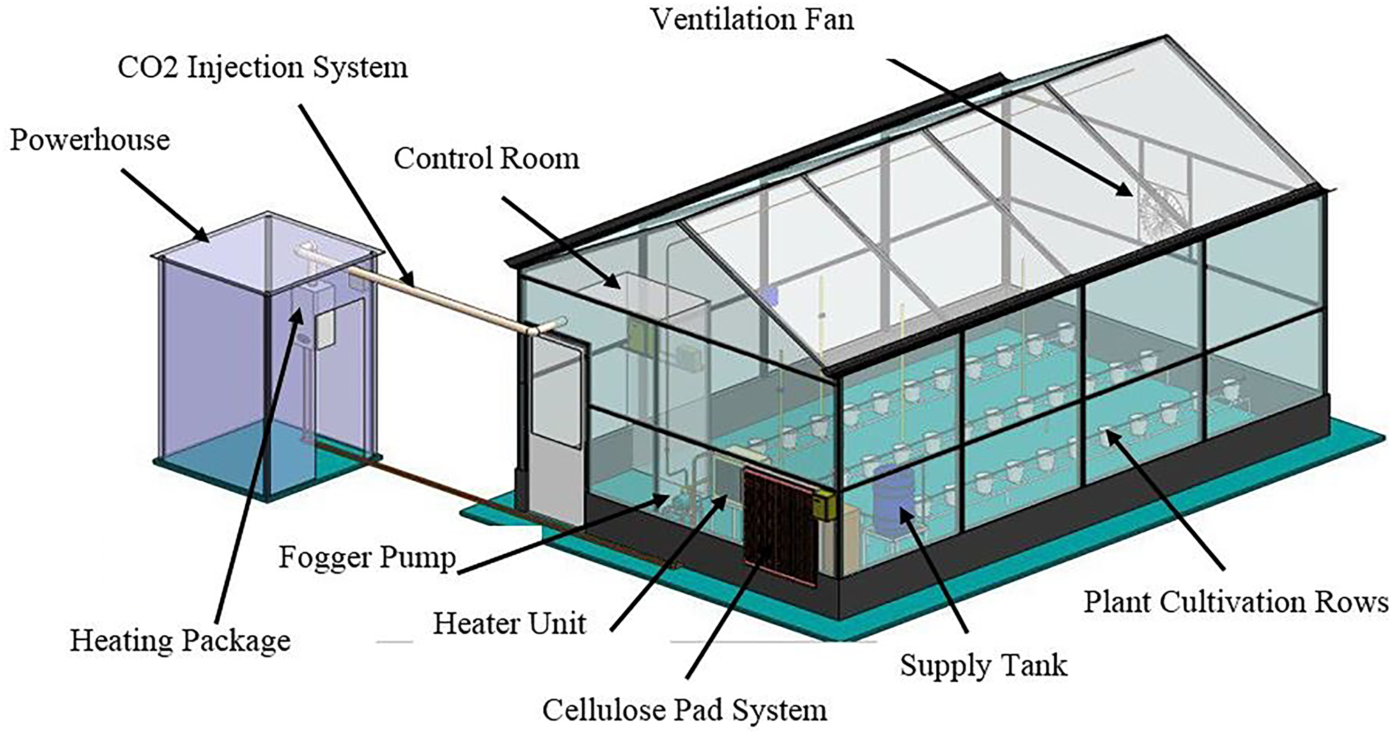
Fig. 1. Greenhouse modelling with SolidWorks software.
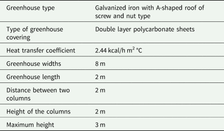
Table 1. Specification of greenhouse
For air temperature and relative humidity sensing, an integrated sensor DHT22 (Aosong (Guangzhou) Electronics Co., Ltd., Guangzhou, China) was used. The DHT22 sensor is also known as AM2302. The K30 sensor, manufactured by the Swedish company Sense Air, is used for the measurement of the amount of CO2 in the air. The GY-302 light sensor module (GY-302 BH1750 Digital Light Intensity Detection) was used for the measurement of light intensity of the greenhouse. This sensor was made in Taiwan (Fig. 2). T 1 to T 4 show the temperature inside the greenhouse, whereas T out shows the outside temperature. Related humidity inside the greenhouse is given by H 1 to H 4, and H out gives its outside relative humidity. L in and L out sensors were installed inside and outside the greenhouse to measure the solar radiation. The temperature and humidity sensor of SHT10 (made in China) was used to measure the plant root moisture. This sensor is fully calibrated and shows high accuracy. The resolution of temperature and relative humidity were 0.01°C and 0.05% RH, respectively. All the data concerning the sensors were stored every 5 s by a control system. The control system board consisted of the power supply board, sensor input board, relay board and main processor board. It was first coded in C++ and then simulated and built with Proteus.
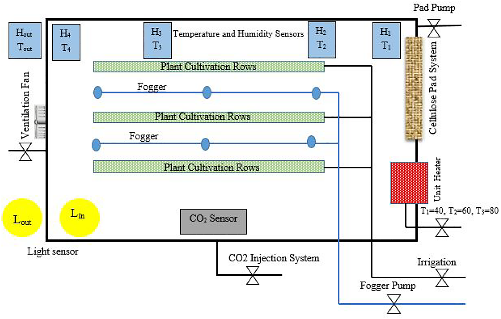
Fig. 2. Greenhouse environment plan.
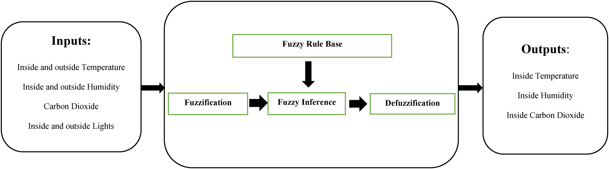
In this research, the greenhouse environmental conditions, including temperature, relative humidity and carbon dioxide, were controlled. The design of a fuzzy controller begins with the selection of the linguistic variables, process status and input and output variables. The next step is to select a set of linguistic rules and the type of fuzzy inference process. The rules are set once, and the fuzzy set and output value need to be specified after the inference, along with the development of a non-fuzzy strategy (Fig. 3).

Fig. 3. Fuzzy logic controller.
An important subject in fuzzy control is the choice of rules, membership functions, number of input and output fuzzy sets and their degree of overlapping, implication and connection operations, and defuzzification method. Fuzzification is the process of converting a crisp input value to a fuzzy value that is performed by the use of the information in the knowledge base. In this study, triangular membership functions are defined for input variables and output variables. The method of defuzzification is the classical method of centre-of-gravity (Revathi and Sivakumaran, Reference Revathi and Sivakumaran2016). In the first phase, a fuzzy control system was extracted from the cucumber growth diagram based on the optimum, maximum and minimum required temperatures of the plant in the greenhouse (Janoudi et al., Reference Janoudi, Widders and Flore1993).
In the current research, a non-circulating or open hydroponic system was used. The cultivation bed was included 60 and 40% of cocopeat and perlite, respectively. Thirty-six pots were arranged in three rows, while the distance between the rows was 1 m and the distance between the row and pot was 0.5 m. Moreover, the pest control was performed during this period whereas weeds and diseases were annihilated by pesticides.
AquaCrop model
Figure 4 shows the main menu of the AquaCrop model. According to this model, weather, crop, management and soil have to be addressed in this model. The variety of the cucumber seed utilized in greenhouse was Karim which is suitable for greenhouse hydroponic plantation. The seeds of cucumber were planted on 25 May of 2019 in the plantation tray and then were planted in the pot on 31 May of 2019.
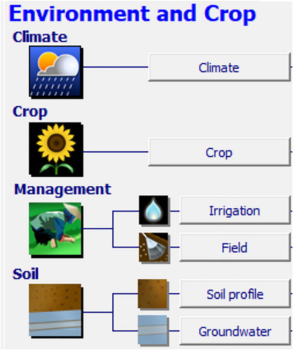
Fig. 4. Schematic of the AquaCrop model (FAO).
The most important climate data for the AquaCrop model are included maximum and minimum temperatures, crop evapotranspiration reference (ET0), rainfall and CO2 concentration. In this study, data from the temperature sensors inside the greenhouse were used for recording minimum and maximum temperatures (Fig. 5(a)). In order to calculate ET0, the Stanghellini model was utilized (Stanghellini, Reference Stanghellini1987). This model uses maximum and minimum daily temperature data to calculate the degree of growth day (GDD) to adjustment biomass yield due to the frost damage (Raes et al., Reference Raes, Steduto, Hsiao and Fereres2009). The data from fogging were used as rainfall data. In the greenhouse, at times where the relative humidity was low, the fogger system worked. The control system recorded the on time of each operator. By recording the data related to spraying, they were calculated as the amount of rainfall in the greenhouse. The annual data for carbon dioxide for various years was available readily in the model (measured by Mauna Loa in Hawaii astronomy) and was not adjustable. In this study, according to the measurement of carbon dioxide in the greenhouse, the closest year that is close to this amount was selected (Fig. 5(b)).
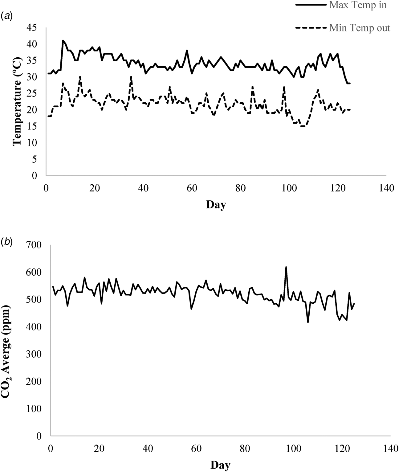
Fig. 5. (a) Maximum and minimum temperature inside the greenhouse. (b) Average carbon dioxide in the greenhouse.
The nutrient solution was provided feed via the hydroponic drip system. In the first step, the nutrient was fed from a reservoir of 100 litres via pipes and drip system. This process is controlled according to a pre-determined programme. To measure the pH and EC of the nutrient solution, a model pH meter (Consort, C650, bljeake) was used. The values of pH and EC were obtained 6.68 and 1.47 g/l, respectively, for nutrient solution.
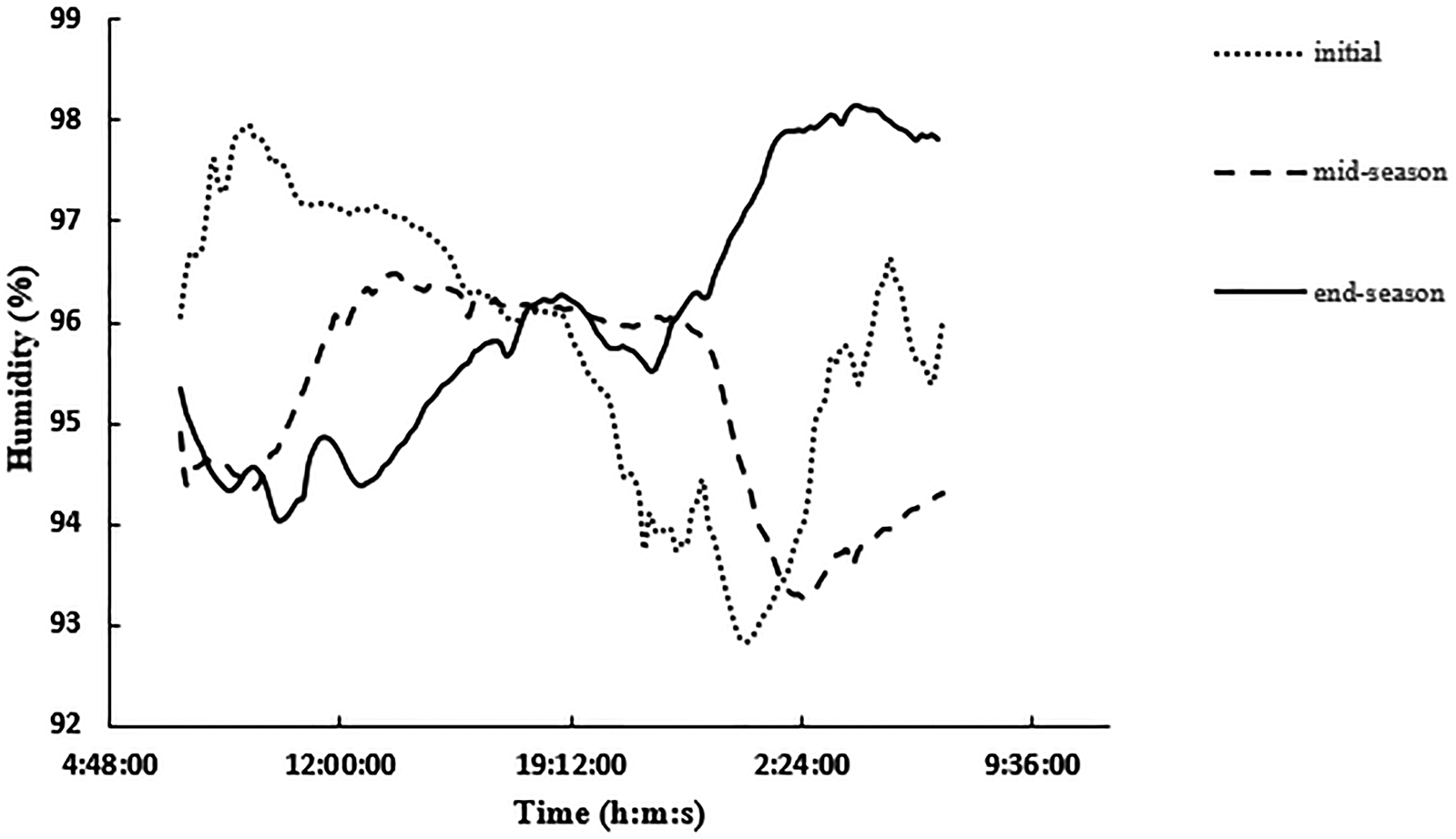
The required data for soil included saturated hydraulic conductivity (K sat), saturated volumetric water contents (θ Vsat), volumetric water contents in field capacity (θ VFC) and volumetric water content at wilting point (VPWP) (θ). Because the planting bed in this research was hydroponic, the sand planting bed with one layer has been used in the model. In AquaCrop, the plant modelled was assumed without having water or fertilization stresses. All the parameters corresponding to location and plant characteristic parameters including water and soil parameters, maximum root depth, plant concentration, planting time and water management were classified into user specific parameters. The depth of soil and its saturated hydraulic conductivity was replaced by 20 cm and 100 mm/h, respectively. In Fig. 6 the planting bed humidity is illustrated in various plant growth periods. As it can be seen in this figure, in the initial stages of growth, the amount of root moisture is higher than middle and end growth seasons, during the day (from 7.00 to 19.00 h). This is due to the plant's low water requirement. As the plant goes to the middle and final growth stages, the plant's water requirement is higher and so the root moisture decreases during the day. The average planting bed humidity is 96.3%.

Fig. 6. Root moisture in the different stages of plant growth.
Estimating evaporation and transpiration
Evapotranspiration (ET) is a fundamental parameter in the greenhouse and shows the sum of water evaporation and transpiration from a surface area to the atmosphere. Evaporation accounts for the movement of water to the air from sources such as the soil, canopy interception and water bodies. In order to find out the exact value for ET, the reference Stanghellini model was used. Accurate estimation of ET is a key parameter in crop/water management of greenhouses. Estimation of evapotranspiration in the greenhouse is different from the estimation of evapotranspiration in the field and the common methods for this case cannot be used. In this paper, the Stanghellini model (1987) was applied to find out the ET in the greenhouse. This model is the revised version of the Penman–Monteith equation based on the status of air velocities in greenhouses (usually low and less than 1 m/s):


where ET is the reference evapotranspiration (mm/day), R n is the net radiation at the crop surface (MJ/m2/day), G is the soil heat flux density (MJ/m2/day), Kt is the unit conversion factor equal to 3600 s/h, VPD is the daily or hourly vapour pressure deficit (kPa), ρ is the mean atmospheric density (kg/m3), Cp is the specific heat of the air $( {\rm MJ\;/kg/}^\circ {\rm C})$ , r R is the radiative resistance (s/m), r c is the canopy resistance (s/m), r a is the aerodynamic resistance (s/m), λ is the latent heat of vaporization (MJ/kg), s is the slope of the saturation vapour pressure curve $( {\rm kp/}^\circ {\rm C})$
 , (is the psychometric constant $( {\rm kp/}^\circ {\rm C})$
 , and LA is the leaf area index (m2/m2).
Some other parameters also have to be considered including net radiation at the crop surface (R n), net short wave radiation (R ns), leaf temperature (T 0) and radiative resistance (r R) (Raeisi et al., Reference Raeisi, Morid, Delavar and Srinivasan2019).
Leaf area measurement as in Eqn. (1) was performed 1 week after transferring the pots to greenhouse. The leaves were separated randomly from three plants. Sampling was executed for 2 months in 7 days intervals. After measuring weight of the leaves, LA was measured by leaf area measuring tool (Delta-T). The LAI was measured by dividing LA to the total occupied area of the plant (row to row distance or plant to plant distance). The LAI was used for calculating the evapotranspiration value of cucumbers.
Results
The results of evaluation for plant parameters
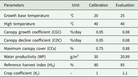
The purpose of calibration is to adjust the plant inputs of the model, which should have the least difference between the predicted values by the model and the actual values. In order to calibrate the model, the data of the first and the second cultivation rows were used for calibration and the data of the third row were used for model validation. Table 2 presents the calibrated parameters of the AquaCrop model. In this study, the crop coefficient for cucumber is 1.1. In this stage, the coefficient WP for producing maximum biomass per unit area, was calculated by two methods of computational and trial and error. In the computational method, the value of this coefficient was obtained by estimating vegetation cover for different stages of growth. Then the daily transpiration was calculated and finally the linear relationship between normalized cumulative transpiration and plant biomass was obtained. In the trial and error method, the coefficient WP was calibrated using the AquaCrop model. Then, the coefficient was changed by trial and error until the simulation results (biomass) had the lowest error compared to the observed values. The obtained values of WP for calibration and validation conditions were 30 and 20.89, respectively.
Table 2. Calibration of model plant parameters for Karim cultivar
Cucumber crop yield and biomass
The recorded agronomic datum was fruit weight (g). Some plants from each pot were randomly selected, harvested and then oven-dried at 70°C to constant weight to determine the above-ground biomass at 125 days. Crop yield was recorded once a week for a cucumber planting period in 2019. Figure 7(a) shows the crop yield of different weeks. The highest value of the crop yield was in the middle of the growth period between 3rd and 6th weeks. After that, by reducing the maximum canopy cover, the yield decreased. The total crop yield of greenhouse was estimated to be ~181.4 kg. In Fig. 7(b), the crop yield of each pot is reported. The crop yield of each plant shows that the environmental conditions created by the fuzzy control system were uniformly throughout the greenhouse. The performance of all pots was almost uniform. The average crop yield of the pot was estimated to be ~5.49 kg. As shown in Fig. (8), the relation between leaf areas and the product crop yield changes in the growth period. This figure shows that the yield increases with increasing canopy cover.
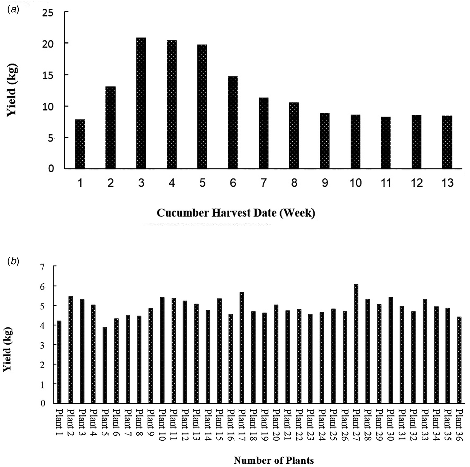
Fig. 7. (a) Hydroponic crop yield of cucumber during the harvest period. (b) Yield of different pots for hydroponic cultivation of cucumber.
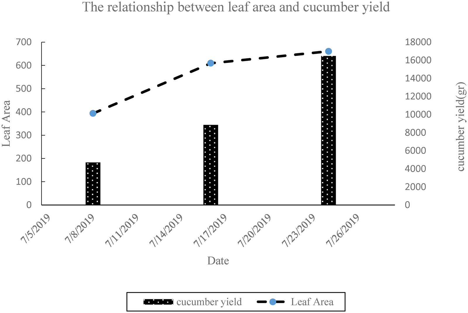
Fig. 8. Relationship between leaf area and cucumber yield.
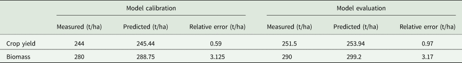
Then the crop yield was estimated by using the AquaCrop model. The data of the first and the second cultivation rows were used for calibration and the data of the third row were used for validation of the model. The comparisons between the real measured values and the predicted values by the AquaCrop model of crop yield and biomass are presented in Table 3. The measured values and the predicted values of the crop yield by the developed AquaCrop model show that the AquaCrop model has predicted the crop yield very well by 0.59 and 0.97 t/ha relative error in calibration and validation process, respectively. Comparison between the measured and predicted biomass via the AquaCrop model for cucumber in calibration and validation phases also shows that the AquaCrop model has simulated the product biomass precisely.
Table 3. Crop yield and biomass values measured and predicted and relative error of the model

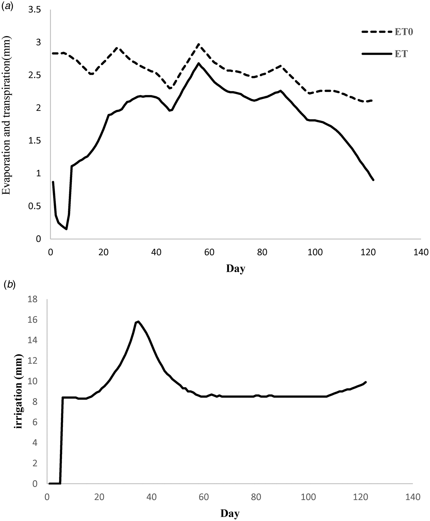
In Fig. 9(a), the reference crop evapotranspiration predicted by the AquaCrop model is illustrated. The results showed that in the beginning of the plantation season evaporation has a greater share in ET because the plants are in the initial stage. This problem shows the importance of evaporation part of E at the beginning of growth season that could be considered in water management in the field. In this phase in order to estimate the evapotranspiration more precisely, separate equations for each growth stage were assigned. The average evapotranspiration in the four stages of initial, development, middle and the end were 1.24, 2.11, 2.15 and 2.05 mm, respectively.

Fig. 9. (a) Reference evapotranspiration and simulated cucumber during the growing season. (b) Cucumber irrigation water requirement with the AquaCrop model.
Figure 9(b) shows cucumber irrigation water requirement estimated by the AquaCrop model. In the early days, because the cucumber seeds did not grow, its irrigation water requirement is zero, and after that, watering the cucumber has started. Irrigation water requirement in the modelling was 1776 mm during the growth period. After that the AquaCrop model evaluates the water requirement of the plant, the irrigation is done according to this requirement.
Discussion
The results of this study indicated that in hydroponic cultivation, due to the use of drip irrigation system, water is provided to the plants on a sub-daily scale according to the amount of water needs, in addition to providing the required nutrients to prevent stress to the plant. So, the proposed AquaCrop model can support the optimized crop production in a fuzzy control greenhouse, including crop management, environmental control, management and sales (Saito et al., Reference Saito, Mochizuki, Kawasaki, Ohyama and Higashide2020).
In the current study, by planting cucumber in a hydroponic greenhouse and measuring environmental and growth parameters, the amount of yield crop and biomass was estimated using a fuzzy control greenhouse and a crop growth model (AquaCrop). Also, the amount of irrigation water consumption of a cucumber crop under hydroponic greenhouse conditions was estimated for the optimal crop production. The results show that the estimated values (2.15 mm) were well simulated compared to the similar studies. Möller et al. (Reference Möller, Tanny, Li and Cohen2004) estimated the evapotranspiration of pepper in the greenhouse in the most consuming season as 2.1 mm in a day.
Because the amount of irrigation varies at different stages of the growth and this requirement can be estimated by crop modelling, an irrigation programme in a greenhouse can improve the amount of water efficiency.
Conclusions
The results showed that the AquaCrop model can estimate actual evapotranspiration with a low error in a greenhouse environment. Also it has estimated the crop yield and biomass with a good degree of precision. Leaf area was measured and it was shown that with increasing leaf area, evapotranspiration rate increased. The results showed that with increasing leaf area, yield also increases. In estimating water consumption, the results showed that in the growth period, the amount of water consumption is almost zero and with the growing of the plant and therefore increasing the leaf area, evapotranspiration consequently increases and results in increasing the amount of water consumption. After the middle growth period the leaf area remained constant, so the daily water consumption remains constant.
Developing the growth model for different greenhouse cultivation can precisely predict the yield and biomass. A major problem in developing control systems is water efficiency and energy efficiency while increasing the yield. Using the growth model in optimizing the control systems is the next step of this process.
Financial support
The authors would like to thank the ‘Iranian National Science Foundation’ for financial support of PhD project with grant number 96011475. The authors are also grateful to the Tarbiat Modares University for financial support given under IG/39705 grant for renewable Energies.
Conflict of interest
The authors declare no conflicts of interest exist.