


Introduction
The Great Recession (from 2008 onwards) stemmed from the USA subprime crisis and involved European countries in two stages: the first involved all northern European countries and the financial sector; the second, after the temporary recovery in 2010, involved the Eurozone, particularly Italy, where the coalition government led by Mario Monti adopted a series of economic austerity measures in the 2011–2013 period in an attempt to promote economic recovery. The crisis deepened in the following years with a sharp increase in unemployment that continued under Enrico Letta's government. This paper analyses the political effects of this economic crisis at a territorial level in Italy.
Bellucci (Reference Bellucci2012) argues that democratic accountability increased in Italy in the decade before the crisis as voters relied less on the long-term anchors which determined voting behaviour, with a decline in the influence of political loyalties and greater influence of social realities.
Voting choices, then, have become more dependent upon the impact of social and, above all, economic performance on the political environment. More responsibility is attributed to the role of the government; hence, there has been an increase in economic voting.
In this paper we choose two electoral outcomes which in many ways defined the Matteo Renzi government. Matteo Renzi was the leader of Democratic Party (PD) between 2013 and 2018 and his government lasted from 2014 to 2016. Indeed, the European elections of May 2014 and the constitutional referendum of December 2016, occurred respectively at the beginning and end of the political parabola of Renzi's PD, and constituted significant tests for the new PD leadership, especially from an economic point of view (Binzer and Wittrock, Reference Binzer and Wittrock2011; Kriesi, Reference Kriesi2012).
At first sight, the European and Referendum election outcomes may look like poor cases to compare, the former being a second-order election and the latter a national referendum. However, we decided to compare these electoral outcomes because in both cases they were considered as political tests of the popularity of Matteo Renzi and the PDs economic policies. There had been, in both cases, a shift of political focus from the effective issues at stake to tests of the political popularity of Matteo Renzi.
Statistical analysis of the voting trends at a territorial level can highlight the determinants of the votes and the political attitude of the Italian voters towards new actors in the new political climate. Our hypothesis is that these electoral attitudes can be explained by economic variables underlying the political votes in the context of the localized cultural milieus. Indeed, two main factors influenced the elections: identity heritage or partisan identification and crisis awareness; both factors are related to the territory, so a territorial approach is particularly useful in this context. The partisan identification is linked to identity heritage, which played an important role, bearing in mind, for instance, the specific territorial area known as the ‘red regions’ or ‘red zone’, historically belonging to the left-wing parties.
During this decade, the economic downturn originated in 2008 with the USs subprime financial crisis which affected many important economic activities in specific territorial areas in Italy. While some industries and areas were resilient, others were hit hard by the economic crisis (Boselli et al., Reference Boselli, Truglia and Zeli2012). This heterogeneity of the resilience to the crisis may explain the rise of electoral spill-over effects in some parts of the country (consistently punishing the incumbent government). Moreover, the economic impact on the Italian production sector was not immediate but displayed all its effects in the years 2012–2014.
The paper is organized as follows: the second section provides an overview of economic voting literature and the third describes the political and economic contexts. The fourth section describes the data, while the fifth describes methodology. The sixth section outlines the results, and the seventh concludes.
The literature on economic and territorial voting
The importance of economic voting is widely recognized by the political science literature (Lewis-Beck, Reference Lewis-Beck1988; Stokes, Reference Stokes and Dennis1992; Lewis-Beck and Stegmaier, Reference Lewis-Beck, Stegmaier, Dalton and Klingemann2007). Economic voting is based on the assumption that rational electors vote for the government parties if the economy is doing well and for the opposition parties if not. Dutch and Stevenson (Reference Dutch and Stevenson2008) hypothesized that economic shocks make the incumbent government's competence evident, and consequently, any successive votes may be informed by economic trends, making the economic vote as important as the ideological vote.
Following Kriesi (Reference Kriesi2012), we can state that political changes depend on the combination of three factors: grievance, organization, and opportunity. The general recession of the decade commencing in 2008 created broad discontent that may have caused a significant shift in voting habits. Although the importance of economic voting is variable over time and the economy is not the only issue relevant to citizens, it dominates other issues in the presence of an economic recession (Singer, Reference Singer2011).
Grievance becomes apparent when voters attribute responsibility for the economic situation to the incumbent government and after they evaluate the economic conditions (Lewis-Beck and Stegmaier, Reference Lewis-Beck, Stegmaier, Dalton and Klingemann2007). In other words, when the voters' awareness of the crisis grows, so does their level of grievance. It is not only the current, personal economic position that matters in economic voting but also the general national economy perception (Dutch and Stevenson, Reference Dutch and Stevenson2008). These perceptions are highly correlated with standard indicators of growth, unemployment and so on.
Economic voters may assess the incumbent government based on a retrospective or prospective approach depending on the political context: if the incumbent party candidate (or the premier candidate of the incumbent party) has a long and clear track record, it will be evaluated on the basis of past facts; otherwise, economic voting will be prospective or forward-looking (Lewis-Beck and Stegmaier, Reference Lewis-Beck, Stegmaier, Dalton and Klingemann2007).
The economic assessment of the incumbent may differ according to many socio-economic factors, such as education, gender, and partisan identification, generating heterogeneity in economic voting according to the intensity and influence of these factors. The factors' impact varies across nations and within nations (Lewis-Beck and Stegmaier, Reference Lewis-Beck, Stegmaier, Dalton and Klingemann2007).
Studies carried out in European countries found that the emergence of mass protest on the streets was generated by austerity measures adopted by incumbent governments (Bartels, Reference Bartels, Bartels and Bermeo2014; Bouvet and King, Reference Bouvet and King2016); therefore, the voters moved from the incumbent to the opposition regardless of whether they were left or right-wing. Moreover, in Western Europe, the beneficiaries of the crisis and the protest vote were the new populist parties. These parties channelled the protests as a form of general opposition to all established parties, and presented themselves as the only real opposition to the traditional party system, giving voice to citizens, and mobilizing them for collective action to improve economic and political conditions.
The transformation of grievance and political mobilization into actual economic voting is normally delayed if a national election is not due in the short run. Economic voting may be exercised in elections at other levels (local, regional, and European) and in national referendums; in these cases, a secondary election can be seen as a test of the national government's performance (Auberger, Reference Auberger2012; Kriesi, Reference Kriesi2012).
Turning to territorial voting, the history of electoral studies can be traced back to two schools of thought: the first focuses on voters' behaviour and their personal motivations, which can be rational (classical theory of rational behaviour of the consumer maximizing his benefits given some budgetary constraints) or psychological (long-term voter loyalty). The second approach highlights aspects linked to the social, economic, and cultural context. In line with the second approach, Durkheim emphasized the importance of constituencies. According to Durkheim, the constituency is ‘a uniform and permanent group consistently present not only at voting day’. In this case, ‘the individual opinion, forming itself within a community, is in turn collectively inspired’ (Durkheim, Reference Durkheim1890–1900). In this framework, elections are important only in the social context in which the voters act. The research carried out in this paper follows the ecological approach and way of thinking that originated in Columbia University (Lazarsfeld et al., Reference Lazarsfeld, Berelson and Gaudet1968). Moreover, as Shin and Agnew (Reference Shin and Agnew2008) point out, political behaviour is either compositional or contextual; the former derives exclusively from individual attitudes (i.e. from socioeconomic attributes), while the latter stems from the mediation of the characteristics of the place where the individuals act, (workplace, residential, and living arrangements), the party origins or immigration from distant places (Agnew, Reference Agnew1996).
The term ‘place’ defines the environment in which individuals act in various contexts. Agnew (Reference Agnew2002: 21) defines place as ‘the cultural settings where localized and geographically wide-ranging socioeconomic processes that condition actions of one sort or another are jointly mediated’. The political behaviour of individuals is acquired in an ever-evolving (and co-evolving) social web in which they are enmeshed. Given the weakening of party affiliation in Europe in recent decades, the vote becomes increasingly contingent, which means that ‘geographical patterns of turnouts and affiliation will become more unstable even as they often still respond to placed-based (but evolving) norms of participation and differing relative attraction to the offering of different parties’ (Shin and Agnew, Reference Shin and Agnew2008: 31).
This paper is aimed to update the literature by considering more recent elections and by analysing the contrast between identity heritage and economic voting. Since all three factors underlined by Kriesi (Reference Kriesi2012): (i) the unfolding of a deep and long-lasting economic crisis that increased political grievances, (ii) the presence of antisystem movements, and (iii) electoral opportunities to make the people's voice be heard, occurred in the Italian political situation between 2014 and 2016, we want to understand how they determine the Italian recent political environment.
We carried out a geo-statistics analysis to comprehend this political evolution in Italy and verify if there is an indication, at a territorial level, of economic voting. Moreover, we aim to understand, again at a territorial level, Italian voters' behaviour in the light of the evidence presented in the literature. Namely, we implement a spatial analysis of some electoral and socio-economic indicators to compare the different situations before and after the Renzi government. In this paper, we consider the unemployment rate as the central economic variable. This indicator reflects both the economic performance of a country and the degree of inequality in its society (if there is no access to employment and income, inequality inevitably increases). A higher unemployment rate directly impacts voters, and it can be calculated at a very detailed territorial level. Summing up, we expect:
– a significant presence of economic voting (i.e. the influence of the unemployment rate on voting patterns), especially for the referendum;
– the manifestation of regional spill-over effects of economic voting driven by:
○ cultural and identity heritage (supporting the Renzi government),
○ the rise of ‘crisis-awareness’ (punishing the Renzi government), that is, a sentiment of economic hardship as opposed to mass-media storytelling;
– the emergence of economic voting and regional spill-over in the Renzi government period due to the escalation of the crisis.
The political and economic scenario
The 17th Italian legislature (2013–2018), witnessed notable political changes which were influenced by wider European economic and social changes. The deepening and widening of the economic crisis in 2011 and the formation of a technocratic government committed to implementing austerity measures led to the emergence of new political movements, and it pushed some parties towards extreme positions; this was the beginning of a new stage of populism. The period was characterized as the ultimate crisis of what had been popularly dubbed (for 20 years) the Second Republic. The Second Republic was based on a two-party system, characterized by competition between a right-wing coalition headed by Silvio Berlusconi's People of Freedom Party (PDL) and a left-wing coalition headed by the PD, the remote heir of the old Communist Party.
After the 2013 elections, two new political players emerged: the Five Star Movement (M5S), an anti-system movement led by the former comedian Beppe Grillo, and a new-look PD led by Matteo Renzi, who dissolved the old guard of the party and assumed the role of innovator in both the PD and the country (Calise, Reference Calise2015).
The clash between these two new actors marked the political struggle in the following years, and it saw the beginning of a new phase sometimes referred to as the Third Republic. It is fundamentally an Italian replication of the struggles between the anti-system movements and traditional governmental forces that have taken place in almost all European Union countries (Kriesi, Reference Kriesi2012). Therefore, it is important to analyse the electoral and political evolution of these forces; Italy might be the laboratory for understanding the future political context in Europe, and it might be paradigmatic for the development of political life in other countries.
In December 2013, Renzi became the leader of the PD with the declared intention of moving the party further towards centrist and liberalistic positions. In February 2014, one of the first steps he brought about was the dissolution of Letta's government and the formation of a new government with himself as Prime Minister and without representatives of the old PD guard.
The new Renzi government was marked by dynamism and new proposals in all fields, from the economy to public education and constitutional revision. In particular, just before the European Parliament vote in May, an 80 Euro cut in personal taxes was granted for the less well-off sections of the working population. Renzi saw the European election in 2014 as a chance to legitimize his leadership by means of a popular vote; moreover, he saw himself as the sole barrier against populism and the political march of the newcomer M5S.
A key element of the new Renzi government was the proposal for constitutional revision overseen by the Minister for Reform, Maria Elena Boschi. This was a far-reaching constitutional reform involving different aspects ruled by constitutional provisions, such as a reorganization of the parliament by substituting the Senate with a Chamber of Regions, some new rules facilitating the introduction of European Union (EU) regulations into the Italian legal framework, the abolition of the regions' right of veto on some specific questions and the strengthening of the Prime Minister's powers. In 2016, since Renzi did not have the qualified majority to approve the constitutional reform in parliament, a referendum became necessary. Renzi saw the referendum campaign as a further legitimation of his leadership and as a test of the popularity of his government's political and economic actions. The resulting campaign was strongly focused on Renzi's political personality (Musella, Reference Musella2015). The opposition took the opportunity to attack him with the aim of weakening and dissolving his government. After the constitutional reform was rejected in the referendum, Renzi resigned as Prime Minister in December 2016 and his government fell.
As regards the economic context we have to note that the economic cycles in the years since 2013 have been marked by highs and lows. The main economic indicators, such as those referring to GDP growth and unemployment rate, improved in the period but still lagged behind the other Eurozone countries.
Both the GDP growth and the decrease in unemployment proved insufficient to make the public perceive a real turning point in the economic situation. Furthermore, while the general unemployment rate was between 11 and 12%, youth unemployment ranged between 39 and 43%.
Unemployment is not spread evenly across Italy. Figure 1 is based on 2011 census data at the municipality level, and it highlights a sharp north-south divide in terms of unemployment with some areas of high unemployment also in the north-east regions. We use the 2011 census data as they are available at the municipal level; this does not affect the validity of the approach because the geographic distribution of unemployment did not change between 2011 and 2014 and 2016. The Spearman ranking correlation indexFootnote 1 is equal to 88.2% for a 2011–2014 and 88.3% for a 2011–2016.
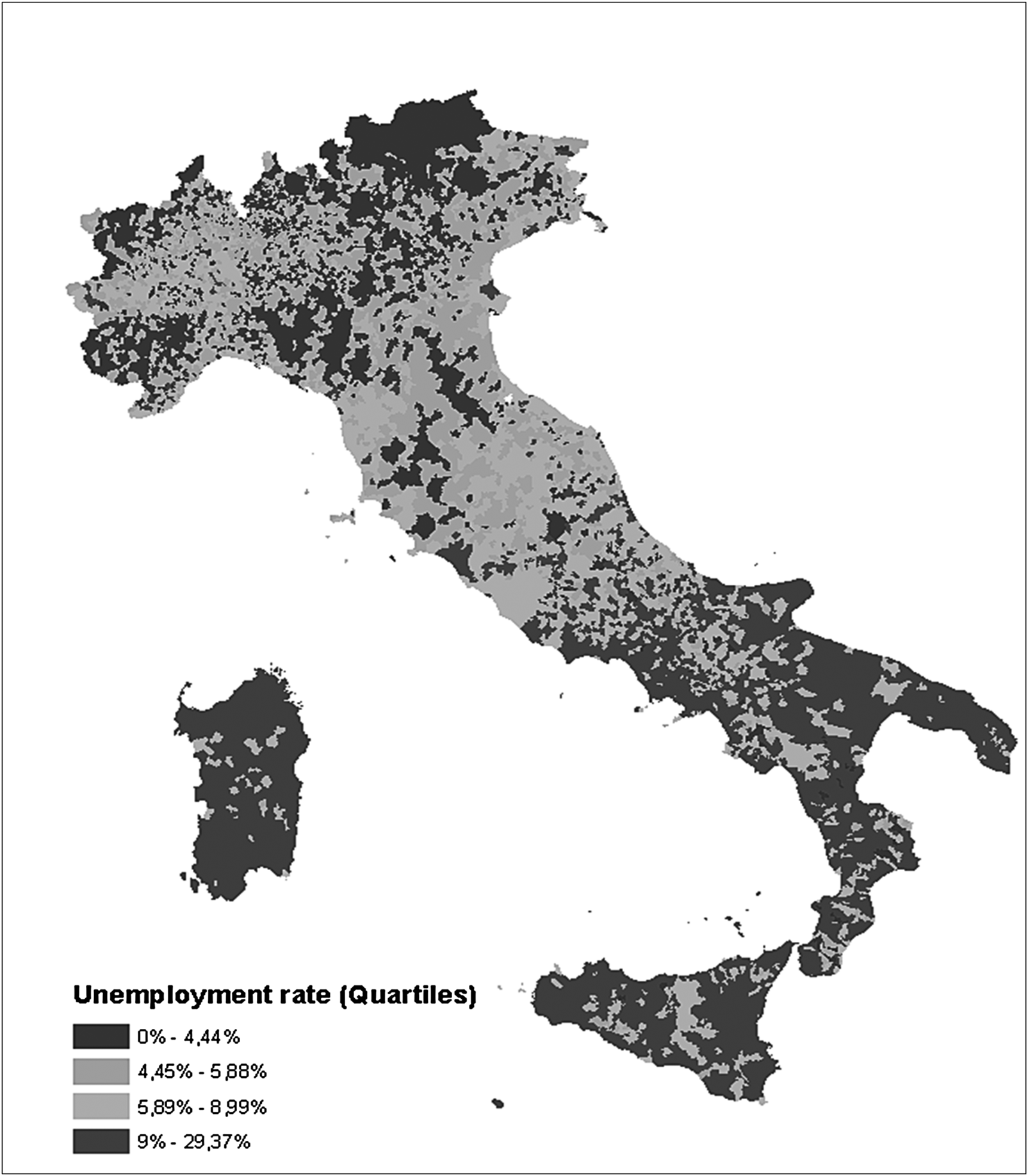
Figure 1. Unemployment rate at the municipality level.
Data and variables
Two data sources, the Ministry of Interior and Istat Census, were used to carry out the analysis. The former includes the results of all electoral exercises from the birth of the Italian Republic in 1946, and are territorially classified. This database is publicly available and provides information on turnout and invalid votes. The latter is the Italian Census of 2011 made publicly available by Istat. The database contains information on the age, sex, education level, employment and unemployment, housing conditions, and the number of foreigners, broken down by territory.
Both databases, linked at the municipality level to yield more information, permit an in-depth analysis of the relationship between votes and economic conditions. The following key indicators are elaborated at the municipal level:
– Youth ratio: the ratio between the number of young people (between 18 and 28 years old) and the total population;
– First time: the rate of first-time voters;
– Tertiary education: the ratio between those who experienced tertiary education and the total population;
– Secondary education: rate of high education level; the ratio between those with secondary and tertiary education to the total population;
– Unemployment rate: the ratio between the number of unemployed people to the total labour force;
– Female unemployment rate: the ratio between the number of unemployed females to the total female labour force;
– Foreigners rate: the ratio between the number of foreigners (mainly immigrants) and the total population;
– Housing conditions: the rate of deterioration of housing conditions; the rate between deteriorating buildings and total buildings.
Regarding the electoral data, we considered the ratio of the number of votes for the PD and the number of votes for other parties in the European election and the ratio of number of votes for ‘Yes’ and the number of votes for ‘No’ in the constitutional referendum.
Many empirical studies use aggregate territorial data (ecological units) and apply it to the whole population, and this needs to be considered when interpreting the results. However, we should avoid the so-called ‘ecological fallacy’ (Robinson, Reference Robinson1950; King Rosen and Tanner, Reference King, Rosen and Tanner2004): interpreting the results exclusively in terms of territorial rather than individual units.
Methodology
The statistical analysis can highlight the factors influencing voting trends in Italy in a new political climate with new political actors. In particular, we aim to explore voting trends through a cultural and economic lens at a territorial level. We carried out a spatial analysis of some electoral and socio-economic indicators to compare the different situations before and after the Renzi government.
The presence of economic voting coupled with a spill-over effect is measured by two different methodologies in this paper. We want to evaluate the importance of economic voting by estimating an econometric model and the prevalence of economic voting with respect to partisan (or identity) voting when economic crises hit. On the one hand, the Moran index permits us to verify the presence and the rise of spill-over effects; on the other hand, the ordinary least squares (OLS) regression is useful to explain the underlying reasons for the areas' aggregation and spill-over at an electoral level.
The Moran index
This paper is based on the hypothesis that electoral behaviour, like other natural or cultural phenomena, spreads via some mechanisms of ‘contamination’ or spatial spill-overs. From a statistical point of view, the data analysis is carried out using spatial analysis data (SAD), in particular, the exploratory data analysis (Anselin, Reference Anselin, Longley, Goodchild, Maguire and Rhind1999).
In the usual regional regression, indeed, the localization of the units of analysis (municipalities) is important, only, from a descriptive point of view. Differently, in the spatial approach the localization units and the structure of spatial contiguity play an important role. They make it possible to identify and describe, with relevant methods (Moran autocorrelation) and models (spatial lag regressions), the units of analysis (municipalities) and the mechanism leading to the territorial ‘dissemination effects’ of electoral behaviour. In territorial data analysis, the units of analysis are usually independent. The SAD approach hypothesizes territorial units' dependence, and this change of paradigm allows for the operationalization of the territory in terms of space and sheds light on the ‘contagion’ mechanism among units.
We choose the Moran (Reference Moran1950) index as a statistical measure of these effects. It registers units' autocorrelation with respect to the intensity of a statistical variable (votes) in contiguous territorial units (municipalities). A major limitation of this index lies in the possibility of exceeding the [−1;1] range (Maruyama, Reference Maruyama2015); moreover, in the case of null autocorrelation, it assumes a value of −1/(N − 1), where N represents the number of observations. The Moran statistics, as other autocorrelation indexes, does not consider the form of unit of analysis and is influenced by the dimension of the areal unit. The topic of the modifiable areal unit problem is very complex and, although connected with the problem of the ecological fallacy, will not be discussed here.
Cliff and Ord (Reference Cliff and Ord1981) detected the probability distribution by which it is possible to build inferential statistics leading to the widespread use of the Moran index. Notwithstanding the limitation highlighted above, this statistic allows the identification and measurement of the spread and spatial effects of social and economic phenomena. Moreover, the Moran index can be broken down into different territorial levels and allows one to identify ad hoc geographical partitions other than a priori territorial hierarchies. Finally, the mathematical structure of this statistic, like the OLS regression coefficient, is comparable to the Pearson's correlation coefficient (Truglia, Reference Truglia2006).
The spatial autocorrelation is analysed by utilizing both the univariate Moran index I (global and local version) and the multivariate index I m defined below. The I and I m statistics record the verse and the strength of the interaction among the ith municipality and its neighbours. The second index, in contrast to the first one, is calculated on two different variables or on the same variable reported at two different times (votes in 2014 and in 2016). This statistic considers, therefore, both the temporal delay (x t−k) and a spatial one (w ijxij), where w ij is an element of W matrix (or contiguity matrixFootnote 2) that represents the neighbouring structure whose elements are encoded as follows:

The index I allows the measurement of instant or contemporary effects, while the statistics I m gives an account of the delayed and dynamic effects of the spatial dependence (Cressie, Reference Cressie1993; Chasco and Lopez, Reference Chasco and Lopez2004).
Pointing out with x t the vote proportions at time t (election 2014), with x t−k the same proportion at time t − k (election 2016) and with w ij the elements of the matrix of contiguity, the index multivariate is

where M is the mean; N is the number of units and S 0 represents the total of contiguity units; the numerator and the denominator represent, respectively, the covariance calculated on the contiguity units and the variance calculated on all units. The ratio between these two represents how much of the variability can be attributed to the territorial configuration of data; and the subscript t − k means the temporal lag when k = 0 the univariate index is obtained.
Contributions from every municipality to the autocorrelation (the global Moran index) are measured by the local Moran index called local index statistics-spatial autocorrelation (LISA):

where (x i − M) is the distance among each category (‘Yes’ or PD vote in the ith municipality) and the average vote; the summation sign represents the dispersion related only to contiguous municipalities; S x2 represents the variance and registers the dispersion degree of the PD/Yes vote with respect to the average; and the LISA statistics signal the units (municipality) that contribute (in a significant way) to the formation of the global autocorrelation index.Footnote 3
Spatial regression analysis
The second application uses a spatial regression model derived from the general one made of the lag-model and the error model. They assess the attraction capacity of a municipality (Cliff and Ord, Reference Cliff and Ord1981; Anselin, Reference Anselin1988). These spatial models can be expressed, in matrix form, as:


where y is the vector N × 1 of the observations of the dependent variable (N is the number of geographical units), W is the matrix of continuity N × N associated with the lag and error variables, X is a matrix N × k of observations of the explanatory variables. Measures ρ and λ are the two (scalar) autoregressive coefficients associated respectively with lag variable y and error factor ε, β is the vector k × 1 of the parameters associated with the explanatory variables X and u is the error term; it shows normal distribution with 0 mean and diagonal covariance matrix Ω.
Since there are three autoregressive terms in the general model (ρ Wy, δ WX, and λ Wε), the OLS method of estimation produces inaccurate estimates with little consistency. The maximum likelihood method (ML) for the parameter estimation is applied:
– with ρ, δ, and λ = 0, to obtain the classical regression model
(6)$${\bf y}\, = \,{\bf X\beta} \, + \,{\bf \varepsilon} ;$$
– with δ and λ = 0, to obtain the error model
(7)$${\bf y}\, = \,{\bf X\beta} \, + \,\lpar {I-\lambda {\bf W}} \rpar ^{-1}{\bf u}$$– with δ and ρ = 0, to obtain the lag model
(8)$${\bf y}\, = \,\rho {\bf Wy}\, + \,{\bf X\beta} \, + \,{\bf \varepsilon} $$


Spatial dependence assumes different meanings according to the applied model (Doreian, Reference Doreian1980). The ρ parameter of the spatial lag represents the relationship among the territorial units in terms of the dependent variable. The model was applied to the European election vote and to the referendum vote. In each case, we estimated the OLS, the spatial lag model, and the spatial error model. For the European election, the model is formulated as follows:

according to the notation specified above. For the referendum, the model is formulated as follows:

where PD is the ratio of votes number for the Democratic Party and the number of votes for other parties in the European election at a municipal level and Yes is the ratio of votes' number for ‘Yes’ and the votes' number for ‘No’ in the constitutional referendum at a municipal level as well. T is a dummy representing geographical areas (North, Centre, and South). The other variables follow the notation specified above. For the spatial lag models, the parameter ρ is also included. Moreover, we estimated the vote change between the two electoral exercises by means of another model having the ratio between the number of votes for ‘Yes’ in the referendum and the number of votes for PD in the European elections as dependent variables and a reduced number of explanatory variables:

The other variables follow the notation specified above.
Results
The comparison of the outcomes for the European elections and the referendum shows that the former was a vote ‘without’ the oppositions' participation, while the latter saw political opponents make their voices (and votes) heard. The European vote in 2014 was characterized by a new political actor (Matteo Renzi) and of consequence by a new personalization of the political debate (Musella, Reference Musella2015); this round of elections was dominated by the ‘benign neglect’ of the right wing, by an attendant attitude of public opinion and by the enthusiastic support of PD militants. The referendum vote came after a couple of years of the Renzi government and low-economic growth. In other words, the novelty had worn off and the effectiveness of government actions was up for debate. The Italian voters had sufficient evidence of government activities to evaluate them.
The voters had to choose between approving the constitutional reform (‘Yes’) or rejecting it (‘No’). The parties supporting the government supported the reform, while the strongest opposition to the constitutional reform came from the Northern League, M5S and some leftist factions. Berlusconi's party was against the reform, albeit with little active commitment to the campaign.
The turnout
The analysis of the turnout provides interesting information. The number of voters increased by 4 million between the two voting exercises. There was a general mobilization of the electorate for both the ‘Yes’ and ‘No’ vote. The southern regions and the Venetian area saw a particularly significant increase, and central regions and Lombardy, above all in the Milan hinterland and in the eastern part of the region, also saw a rise in voter turnout. While the central regions are the PDs traditional electoral background, Lombardy is traditionally Berlusconi's stronghold. It seems that at least a part of Berlusconi's PDL electors may have voted ‘Yes’ despite the ambiguity of Berlusconi's position. Between the European Parliament election and the referendum, there was a shift from abstention to a ‘No’ vote. We calculated the difference between the European Parliament election and referendum abstentions and between the ‘Yes’ and ‘No’ votes. The correlation between these differences is equal to 94%. It shows a movement of undecided voters to a more engaged attitude in the second electoral exercise.
The electoral exercises and the Moran index
The analysis of vote distribution by municipality confirms there was more opposition in 2016 than in 2014. The distribution of votes for PD and the votes favourable to constitutional reform (‘Yes’) are shown in Figure 2. When comparing the two maps we can note a dark grey zone, almost unchanged between the two electoral exercises, covering the central regions south of the river Po. This is the traditional, so-called ‘red zone’ where the old Communist Party (PCI) obtained the majority of votes and has its main cultural and economic roots. The PD inherited this block of votes directly from the former Italian Communist Party (PCI). In the ‘red zone’, almost all municipalities and regional councils are dominated by the PD, and many cooperative societies linked to the PD were founded and operate in these regions.

Figure 2. PD and Yes vote distribution.
The rest of the northern regions (north of the river Po) are split into two areas: the north-west and the north-east. The former is composed of Piedmont and Lombardy; it registered a strong increase in the shadowed areas, in other words, the public support towards the PD stance increased. The latter is composed of the Venetian and Friuli provinces; in both 2014 and 2016, there was unwillingness there to vote for PD.
However, the most interesting fact is the sharp division between the north and south of the country. We can distinguish a line across the centre of Italy dividing the ‘red zone’ from the rest of the peninsula, including Rome and the islands of Sicily and Sardinia. The latter are the more economically disadvantaged areas of the country. Between the 2014 and 2016 electoral exercises, the PD further lost public support in the southern regions. Moreover, the southern margin of the red zone was eroded, and the PD lost some border areas.
To sum up, the distribution of votes by municipalities identifies four zones:
– the PD ‘hard core’ zone, which is represented by the red regions of central Italy where the PD did not lose support;
– the north-west area, where the PD consensus gained some public support between the two electoral exercises;
– the Venetian region, that represents long-standing opposition to the PD;
– Rome and the South, where the opposition to the government strengthened in the period between the two electoral exercises.
Figure 3 presents the results for the Moran index elaborations for the European election and the constitutional referendum, respectively. The Moran index is, in both electoral exercises, positive and signals that municipalities have a medium-high tendency to aggregate themselves according to the variables considered. The value of the Moran index for the two electoral turns is respectively 0.33 and 0.39, in both cases these values are significant (P < 0.01).

Figure 3. Moran index – PD and ‘Yes’ vote distribution.
The LISA index highlights six types of territorial aggregations, the two most common of which are displayed in dark grey and black where the creation of municipalities' cluster (territorial spill-over) is strongest.
The municipalities coloured in dark grey (HH) are the areas (or contiguous municipalities' clusters) with a high support for PD/Yes, the municipalities coloured in black (LL) constitute clusters of contiguous municipalities with low support for PD and a lower percentage of ‘Yes’ votes. The local Moran index represents well the contrast between the aggregation zones of PD voters and the aggregation zones of non-PD voters as well as the ‘Yes’ and the ‘No’ voter zones.
The vote for the PD is substantially stable in the centre (the ‘red zone’), and changes dramatically in the southern regions: (the Rome area), almost all of the Naples' region (Campania), a large part of the south-east (Puglia) and above all the main Islands (Sicily and Sardinia), from a broadly neutral situation to one of direct opposition. These areas saw strong support for the PDL and the Northern League (Shin and Agnew, Reference Shin and Agnew2008), although a large part of this support now goes to M5S, especially in the southern regions. In the north, the PD made the most gains in the most northern region (Trentino), while the traditional zone of opposition to PD (the Venetian zone) further enlarged its borders. In the north-west, we can see a resilience of PD positions or even an enlargement of its influence. The comparison over time of the Moran index results reveals two poles: one representing a traditional cultural heritage (leftist), the other the incoming aggregation of a new sentiment that we could call ‘crisis-awareness’. These poles, as well as being psychological attitudes, represent political orientation that takes root in specific areas of the national territory. In particular, we can note the presence of a great spill-over effect in central Italy due to a long-standing traditional cultural heritage of Communist Party support and the presence, in other regions more affected by the economic crisis, of a new phenomenon of electoral spill-over due to the consequences of the crisis itself. The bivariate Moran index for PD and ‘Yes’ votes is presented in Figure 4.

Figure 4. Overlapped Moran index – PD and ‘Yes’ vote distribution.
Although the representativeness is lower with respect to the univariate Moran indexes, we can distinguish the same areas detected previously. The analysis of the vote by means of the bivariate Moran index substantially confirms that the votes can be territorially classified in the four zones described above: the north-west, the Venetian region, the ‘Red regions’ (Central), and Rome with the South.
It is worth noting the prevalence of the PD/Yes vote in the inner-city areas and the loss of this prevalence in the suburbs in Turin, Milan, and Naples. This is also the case in Rome but the municipal administrative borders do not allow clarity of this effect. The centre-suburbs vote differentiation is important because it marks a social and economic differentiation between the affluent centres and the zones most economically affected by the crisis.
Another important point is that the only zone in which a certain gain for the ‘Yes’ is observed is the north-west region in Milan and in the Lombardy foothills of the Alps. These zones are a traditional political stronghold for Berlusconi's PDL; this suggests that, for the referendum vote, an important quota of right-centre voters switched to the PD position (‘Yes’) despite Berlusconi's lukewarm support of the ‘No’ thesis.
Economic and social analysis of electoral exercises
Statistical spatial regressions were estimated to understand and evidence the relationship between economics and votes. The usual diagnostic for spatial dependence, Robust LM (lag) and Robust LM (error), was implemented; in both cases Robust LM (lag) is greater than Robust LM (error), this is a confirmation of the correctness of the spatial lag model with respect to the spatial error one (Table 1).
Table 1. Economic voting impact for the European elections and the referendum

(*)For European Election Model 9 is estimated and model 10 for Referendum.
(**)In Italy the numbers of municipalities is 8092 but for some of them (the smaller ones) the data are non-available.
In regression (2) the vote for PD (ratio between PD and non-PD votes) in the European election is negatively affected at a municipal level by the rate of youth and by the incidence of first-time voters, while the social and economic variables are not significant; only the Foreigners rate is strongly significant and positive. This means that the presence of foreigners (legal immigrants) does not negatively influence the vote for the PD. It is worth mentioning that neither the Unemployment rate nor the rate of deterioration of housing (housing conditions) is significant. It is interesting to compare these results with column (4). In this case, we are regressing on the ratio between the ‘Yes’ and ‘No’ number of votes in the constitutional referendum as a dependent variable.
The youngers' vote coefficient is not significant, while the first-time electorate voted ‘Yes’. At the municipality level, the more educated people (tertiary education) voted against the proposed change of constitution. It is important to note that the unemployment rate coefficient is negative and significant. The female unemployment rate remains non-significant, as does the housing conditions coefficient. The territorial dummy is significant both for the North and for the Centre. The reduction of the Centre coefficient for the referendum and the increase in the North coefficient confirms the PD losses in the red zone of the centre and the gains in some northern zones such as Milan and central Lombardy. To sum up, the indicators, together with the analysis carried out above, in the ‘Turnout’ sub-section, tell us that the referendum represented an opportunity to mobilize the electorate; the referendum was represented by both political sides as a battle of ideas and this has led, together with economic unrest, to a greater turnout with respect to the European election vote.
The spatial dimension of the variable PD/Yes measured by ρ for spatial lag model, confirms the tendency of territorial clustering of municipalities and the presence of a high degree of territorial spill-over. This result stresses the central role played by territory in contrast with the historical tendencies towards a dematerialization of the political, economic, and social frameworks. The vote variations are outlined in Table 2.
Table 2. Economic voting changes between PD and Yes votes

(*)Model 11 estimations.
(**)In Italy the numbers of municipalities is 8092 but for some of them (the smaller ones) the data are non-available.
The time trend already presented in the estimation of models (9) and (10) is substantially confirmed at a territorial level.
The dependent variable is the ratio between the number of PD votes in the European elections and Yes votes in the referendum in the same municipality. We considered only the significant variables in the previous models. The analysis revealed that, in the municipalities with higher unemployment rate and education, the ‘Yes’ vote is lower, while a reverse relationship seems to occur for younger voters'. Finally, we have an increasing effect of the presence of immigrants on votes causing a slight increase in Yes/PD voting in the north.
Conclusions
We carried out a statistical analysis of two important electoral exercises in Italy: the European elections in 2014 and the constitutional referendum in 2016. These electoral exercises in many ways defined the Renzi government's term of office, so it is possible to interpret the electoral results as a public evaluation of Renzi's government, especially in terms of its economic policy.
Two statistical analyses were carried out. The first one was based on an original Moran index; it yields the context of aggregative/repulsive processes at a territorial level for the two electoral exercises. The other one, based on spatial regression techniques, analysed the relationship between votes and economic and social variables at a territorial level. The two types of analysis converge to show that the social and economic factors influenced the vote and steered public opinion.
The influence of these factors became greater as ‘crisis awareness’ grew, and a retrospective approach was prevalent in the voters' behaviour. In fact, the comparison of the analysis over time highlights the differences in the electorate's behaviour between the two electoral exercises.
In the municipality with a higher abstention rate and a higher rate of unemployment, the 2014 vote for PD was not negatively influenced. This seems to demonstrate that the electorate gave the new government a chance by voting for it directly or by not voting at all if holding allegiance to another political party.
The comparison of the Moran index analysis over time indicates the presence of a regional spill-over effect in central Italy due to traditional cultural heritage (leftist) that is not closely linked to economic voting for both electoral exercises. This is despite the fact that these areas showed strong economic resilience to the crisis (Boselli et al., Reference Boselli, Truglia and Zeli2012). The presence of a regional spill-over effect of economic voting on the incumbent government is registered only in the referendum. The Moran index shows the emergence of regional spill-over effects in different areas and, if the regression results are compared with the Moran index results, it can be noted that the more disadvantaged zones, the South, or the areas most affected by the economic crisis, the North-East (Boselli et al., Reference Boselli, Truglia and Zeli2012), are the same areas with the lowest numbers of ‘Yes’ votes. The regression results verify, at a very detailed territorial level, that the referendum result is influenced by the economic vote and that the emerging regional spill-over effects against the government policies are driven by economic reasons. The areas in which the regional spill-over of the ‘negative’ economic vote is stronger may be defined as aggregations of a new sentiment that can be called ‘crisis-awareness’.
The spatial regressions indicate that in the areas in which the unemployment rate is higher it negatively influences the ‘Yes’ vote in the same areas; while the rate of housing conditions deterioration in this case does not appear to affect the change in electoral behaviour perhaps because it expresses a form of social unrest which is older and layered over time.
The government's defeat in the referendum can be traced back to economic factors: the absence of perceived economic improvements and the persistence of high unemployment. Apart from the substance of the constitutional reform, which represented an important factor of aggregation of political forces opposing the government, the statistical results demonstrate that social and economic variables directly influenced the political engagement and steered the vote. The geographical patterns of affiliation became more tenuous, the voting choices were largely the result of the influence of economic performance on the political environment and, finally, economic voting prevailed, increasingly, over partisan voting (Truglia, Reference Truglia, Fruncillo and Addeo2018).
Data
The replication dataset is available at Italian Political Science Review (IPSR/RISP) Dataverse (Società Italiana di Scienza Politica and Cambridge Journals).
Financial support
This research received no grants from public, commercial, or non-profit funding agency.


