Requirement (a): establishing sufficiency for explanatory purposes

As a technique, QCA relies on an algebra of set that preserves the equivalence to a first-order logic (Stone, Reference Stone1936). Thus, the technique addresses Simon's knowledge problem – the determination of the truth or falsity of P – as the problem of gauging a unit's membership in the set of things that are or have P (e.g. Sartori, Reference Sartori and Id1984; Ragin, Reference Ragin2008; Goertz and Mahoney, Reference Goertz and Mahoney2012; Ragin and Fiss, Reference Ragin and Fiss2017). QCA affords two such gauges: crisp and fuzzy. The crisp gauge assigns binary truth values in line with the Boolean canon: the 0-membership in p means 1-membership in the negated set ${{\bar{P}}}$. The fuzzy gauge refines the assignment with that which, from an explanatory perspective, can be understood as an ambiguity penalty. Fuzzy scores incorporate such a classification error in the value assigned to each unit. They span from 0.00 to 1.00 and have their point of highest ambiguity at 0.50: thus, units scoring 0.50 are instances of neither p nor ${{\bar{P}}}$; units with extreme values, instead, are sure instances of either a set or its negation.

The difference in gauging slightly changes the operationalization of the three logical axioms on which QCA can build valid causal claim. As summarized in Table 1, the three rules establish, respectively, the negation of a state as its arithmetic complement in the universe of reference; the rule of non-contradiction as the impossibility for the same unit to be in a state and its negation at the same time; the rule of the excluded middle as the necessity of a unit to display either one or the other of the two possible states. These gauges allow enforcing the conventional understanding of sets as ‘conceptually uniform’ partitions of the universe with respect to a condition's state.

Table 1. Axioms, set renderings, and gauges

Notes: ψ ^cs is for the crisp-set membership score, ψ ^fs is for the fuzzy-set membership score.

$\psi _{P_i}$refers to membership score that the i-th unit from a universe ${\cal U}$ of size N takes in the set of instances sharing the condition P in a state; $\psi _{{\bar{P}}_i}$ is the membership score of the same unit in the set of the condition in the negated state.

The overbar here reads ‘not’. The alternative notation in QCA is the curl ~, or the lowercase set name.

The backlash \ indicates the set difference.

$\cup$ reads ‘union’ and corresponds to the logical inclusive (weak) ‘or’. The alternative logical notation is the vee ∨; in QCA's applications, it is common to use the plus sign +.

$\cap$ reads ‘intersection’ and corresponds to the logical ‘and’. The alternative logical notation is the wedge ${\wedge}$; in QCA's applications, the operator is a dot (⋅) and often omitted.

$\emptyset$ indicates the empty set; the corresponding logical notation is the empty curly braces. QCA conventionally renders it with a 0, although 0 is also assigned to the ‘fully out’ observed instance.

The construction of sets as uniform partitions provides the ground of the set-theoretical gauge of sufficiency. The relationship is, quite conventionally, a conditional. The parameter that captures it in any QCA application is the ‘consistency of sufficiency’ (S.cons for short: Ragin, Reference Ragin2000, Reference Ragin2008; Duşa, Reference Duşa2018). The parameter is defined as the ratio of the size of the intersection of the outcome and a primitive, and the size of the primitive itself: $S.cons_{\omega _j{\it{\subset Y}}} := \vert {\omega_j {\it{\cap Y}}} \vert / \vert {\omega_j} \vert$. It closely recalls Kolmogorov's measurement of conditional probability as the ratio of success to trials of a certain kind (e.g. Hájek, Reference Hájek, Bandyopadhyay and Forster2011). Indeed, without any loss, the $S.cons_{ \omega _j {\it{\subset Y}}}$ can be rewritten as π(y|ω _ji), being π the size of the sets; in the special case of crisp QCA, the size of the set is the number of its instances and Kolmogorov's conditional probability coincides with the consistency of sufficiency. In both cases, moreover, the parameter renders the long-honored regularity criterion that ‘if ω _j causes y, then any instance of ω _j is an instance of y’; at the same time, it accounts for the challenge that contradictory evidence rises to the modal understanding of causal regularity as ‘if ω _j causes y, it cannot be the case that an instance of ω _j is an instance of ${{\bar{Y}}}$’.

The regularity claim of the S.cons stands when the parameter takes either its highest value of 1.00 or its lower value of 0.00, indicating that the primitive draws a uniform partition of the positive or the negative outcome set. For explanatory purposes, violations of this subset relationship make the primitive ‘contradictory’. Contradictions weaken the claim that the team of conditions renders an inus machine, and suggest that the team is ill specified – possibly, due to some omitted components. From a logical perspective, a contradiction makes the inus hypothesis ‘false’, as its realizations cannot establish the subpopulation of y-instances as a separate set from that of ${{\bar{Y}}}$-instances.

The diagnosis of the contradiction through the S.cons is straightforward with crisp scores (Rihoux and De Meur, Reference Rihoux, De Meur, Rihoux and Ragin2009) but can prove harder with fuzzy scores. The violation can be downgraded to an acceptable inconsistency when it arises from units for which Y _i ≥ ω _ji + 0.1 (Ragin, Reference Ragin2000); truly contradictory instances instead remain those crisp consistency outliers for which ω _ji > 0.5 while y _i < 0.5 (Rohlfing and Schneider, Reference Rohlfing and Schneider2013; Rubinson, Reference Rubinson2013; Rohlfing, Reference Rohlfing2020). The misalignment of the crisp and the fuzzy consistencies depends on the fuzzy scores leaving arithmetic residuals in intersections: to witness, $\psi _{P} ^{\rm fs} = 0.8$ yields $\psi _{( {P_i \cup {\bar{P}}_i} ) }^{\rm fs} = 0.2$, which indicates an empty intersection by the rules in Table 1, yet inflates the diagnostic of the S.cons. To overcome the problem, a corrected version of the parameter has been devised. The Proportional Reduction of Inconsistency (PRI), calculated as $PRI_{\omega _j {{\subset Y}}} := \vert {\omega_j {{\cap Y}}} \vert - \vert {\omega_j {{\cap Y \cap \bar{Y}}} \vert / \vert {\omega_j} \vert - \vert {\omega_j {{\cap Y \cap \bar{Y}}}} \vert}$, explicitly borrows the rationale of the Proportional Reduction of Error. The gauge of inconsistency is $\vert {\omega_j {{\cap Y \cap \bar{Y}}}} \vert$, which assigns higher penalties to fuzzy values of the outcome closer to 0.5. The PRI, hence, displays a steep fall in the values of the parameter, often for primitives with S.cons equal to 0.85 or lower. The convention maintains that a configuration is usually sufficient to an outcome when its S.cons is 0.85 or higher and supported by a similar PRI – although model specifications may suggest otherwise (Schneider and Wagemann, Reference Schneider and Wagemann2012).

Requirement (b): handling the overspecification of inus machines

The additional relevant information in Standard QCA comes from the coverage of sufficiency, or S.cov for short, defined as $S.cov_{\omega _j {\it{\subset Y}}} := \vert {\omega_j {\it{\cap Y}}} \vert / \vert {\it{Y}} \vert$. The parameter indicates the empirical relevance of the realization ω _j to the instances of the outcome y (Ragin, Reference Ragin2006, Reference Ragin2008). It takes its highest value of 1.00 when the j-th realization is shared by all the instances of Y and tends toward 0.00 the more there are instances of the outcome set (ψ _Y > 0.50) outside the configuration set $( \psi _{\omega _j} < 0.50)$.

The raising of uncovered instances may follow from omitted alternative paths to the outcome (e.g. Rohlfing and Schneider, Reference Rohlfing and Schneider2013; Oana and Schneider, Reference Oana and Schneider2018). Usually, their presence is deemed of little or no threat to the standing of a consistent hypothesis. If we are only interested in the machine triggered by our model, any uncovered instances of y can be a red herring. However, coverage outliers can have another and more concerning source. They are also diagnosed on the overspecification of the model that occurs when unrelated conditions are added. In explanatory QCA, the minimization algorithm offers a strategy to handle this threat while providing an argument in favor of the often-deplored practice of selecting on the dependent (e.g. King et al., Reference King, Keohane and Verba1994: 130). Indeed, a renowned ‘paradox of confirmation’ illustrates the absurd conclusions that standard analyses can reach when blindly applied to instances selected on a ‘wrong’ independent (Salmon, Reference Salmon1989: 50).

The paradox portrays the case of the table salt that is believed to dissolve (y) once put in hexed (h) water (w). The underlying inus model, then, reads ${\it{H \cap W \to Y}}$. The paradox arises as natural diversity presents us with the primitives as in Table 2.

Table 2. Truth table from the model ${\it{ H \cap W \to Y}}$

An analysis narrowing on π(Y|ω ₁) would consider the relationship sound, even by contrast with π(Y|ω ₄). The proof of the irrelevance of ${{\bf H}}$ emerges from the evidence that π(Y|ω ₁) = π(Y|ω ₃) and π(Y|ω ₂) = π(Y|ω ₄), once the distinction is made between hexed and non-hexed water. Under the improved model specification, the comparison of configurations to the same outcome pinpoints the irrelevant component as the one whose variation does not affect the state of the outcome. Its removal follows from a logical operation that the original pruning algorithm of QCA, the Quine-McCluskey, performs systematically. To witness: in Table 2, the non-contradictory antecedent of ${{{Y}}}$ is ω ₁, ω ₃; hence, we can rewrite the solution of ${{{Y}}}$ as $( {{{H\, \cup\, \bar H}}} ) {{W}}$. By the axioms in Table 1, ${{H\, \cup \,\bar H}\, =\; {\cal U}}$; hence, h can be dismissed as ‘noisy’ background variation. Run on the instances of y, then on those of ${{\bar{Y}}}$, the operation licenses the conclusion that the non-irrelevant implicant of ${{\bf \it{Y}}}$ is ${\it{W}}$ and that the inus model is truer to the cases at hand when specified as w → y.

Addendum to requirement (b): handling unobserved realizations

The previous example has assumed a saturated truth table in which all the possible realizations were observed. Technically, observed realizations are those in which at least one unit has a crisp membership score of 1. In actual explanatory QCA, however, an inus model easily allows for a wider array of realizations than the units may afford from a certain universe. The problem is understood as ‘limited diversity’ and provides a further version of the curse of dimensionality. It is independent of the mere ratio of the number of cases and variables, and may not be properly addressed by adding cases: infinite instances of the same primitive in an analytic space of four still make three primitives unobserved and provide no analytic leverage.

The strategies to handle unobserved realizations are many, each addressing a possible source of the problem. Observed diversity may increase if we widen the space-time region of the analysis – the ‘scope condition’ for case selection (Marx and Dusa, Reference Marx and Dusa2011). The dimensionality of the analytic space can decrease if some gelling interactions are hardened into measures of coarser factors (Berg-Schlosser and De Meur, Reference Berg-Schlosser, De Meur, Rihoux and Ragin2009; Schneider, Reference Schneider2019). If inadvertently added, empirical constants may be dropped before the analysis of irrelevance as they double the analytic space but leave half of the primitives unobserved (Goertz, Reference Goertz2006).

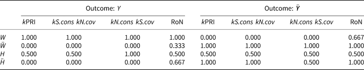
The latter consideration has evolved into a whole step of the standard protocol. The ‘analysis of individual necessity’ calculates the same parameters as the analysis of sufficiency, but of conditions and with a reverse meaning. Constants are degenerate necessary conditions, that is, limiting cases of supersets of an outcome-set. They arise when |Y| ≤ |P| and entail a lower-triangular fit. The membership in the condition given that in the outcome renders the individual consistency of necessity ($kN.cons_{{\it{Y \subset A}}}: = \vert {\it{A \cap Y}} \vert / \vert {\it{Y}} \vert$), whereas the membership in the outcome given that in the condition provides the individual coverage of necessity ($kN.cov_{{\it{Y \subset A}}}: = \vert {\it{A \cap Y}} \vert / \vert {\it{A}} \vert$ )– where ‘individual’ is referred to the k-th inus condition. The Relevance of Necessity ($RoN_{{{Y \subset A}}} : = \vert {{\bar{A}}} \vert / \vert {{\bar{A} \cup \bar{Y}}} \vert$: Schneider and Wagemann, Reference Schneider and Wagemann2012) is a later addition aimed to verify the meaningful variation of each inus components. It is calculated as the reciprocal of the membership in the unrealized outcome conditional on that in the unrealized factor. The standard recommendation is to consider dropping as trivial the factors with kN.cons close to 1.00 and low RoN. However, the crucial test and consistent with the inus rationale remains whether the model requires any seemingly trivial condition to prevent the rising of contradictions in the truth table (Damonte, Reference Damonte2018; Rohlfing, Reference Rohlfing2020).

However, the protocol of reference to handle limited diversity is that of the standard minimizations that treat unobserved primitives as counterfactuals (Ragin, Reference Ragin2008; Schneider and Wagemann, Reference Schneider and Wagemann2012) and, ultimately, a problem of missing outcomes. The related counterfactual question asks whether any instance of these configurations, known yet unobserved, would have displayed y instead of ${{\bar{Y}}}$ (Ramsey, Reference Ramsey and Mellor1929). The standard protocol provides three answers – ‘conservative’, ‘parsimonious’, and ‘intermediate’ – and draws its conclusions under as many alternative assumptions.

The conservative stipulates that no unobserved realization would have obtained; so, its minimizations only operate on observed diversity. The parsimonious maintains that any unobserved realization would have obtained that finds a perfect observed match but for a single minimizand – the component to be declared irrelevant. The intermediate corrects the parsimonious assumption with plausibility concerns. It requires the unobserved minimizand to be in the state that the inus theory considers ‘right’ to the outcome. The minimization under such ‘directional expectations’ provides the intermediate or ‘plausible’ solution. Given all non-contradictory primitives, the conservative and the parsimonious solutions provide the tighter and looser boundaries of a ‘confidence solution space’ in which the intermediate solution usually offers the plausible estimate to the best of knowledge – with a caveat.

Concerns have been raised that directional expectations might introduce confirmation bias in solutions. Minimizations are geared to disconfirming the relevance of a component of the model, not to establish it; so, relying on directional expectations to drop a term rather uses the theory against itself. Instead, the blind application of the plausibility rules may arise a different version of the ‘paradox of confirmation’ in which the belief in a wrong theory prevents the dropping of irrelevant conditions from the solution.

To witness, let us take the hexed salt example of Table 2, but now with an unobserved realization, $\omega _3^\ast \colon {{\bar{H}W}}$ in Table 3. Let also assume that our directional expectations about ${\it{H}}$ reduce to the belief that, teamed with the right inus factors $ {\Phi}$, hexing is an inus component of the machine to y when present: $ {\it{H}} \Phi {{\subset Y}}$.

Table 3. Truth table of ${\it{H \cap W \to Y}}$ with unobserved ω₃

Given Table 3,

• – ω ₁ is the only realization to $ {{Y}}$, and the conservative solution reads $ {{HW}}$: the salt dissolved because it was hexed and in water.

• – the parsimonious minimization matches ω ₁ and $\omega _3^\ast$ and yields $ {{W}}$ as the prime implicant: the salt dissolved just because in water.

• – the intermediate minimization considers that $\omega _3^\ast$ is an implausible or ‘hard’ counterfactual instead, as it carries the minimizand in the wrong state according to the directional expectations. Thus, $\omega _3^\ast$ is barred from the minimization with ω ₁; the resulting plausible solution overlaps the conservative, and the irrelevant factor is not dropped.

To some, the proven inability of the intermediate solutions to get always rid of known irrelevant components disqualifies it as valid, and leaves the parsimonious solutions as the finding to be discussed (e.g. Thiem, Reference Thiem2019). To others, parsimonious solutions are too dependent on observed realizations, and their sufficiency far less ‘robust’ when tested on shrinking diversity for providing a reliable result (e.g. Duşa, Reference Duşa2019). Besides, plausible assumptions are required to make complete structures emerge (e.g. Fiss, Reference Fiss2011; Damonte, Reference Damonte2018; Schneider, Reference Schneider2019).

The debate disregards the possibility that data contain handy information to establish the plausibility of the inus theory. The values of the analysis of individual sufficiency provide indications on the tenability of our directional expectations in ${\cal U}$. When calculated on the conditions of the hexed salt as in Table 4, the kPRI and the kS.cons values show h being equally insufficient to y and $ {{\bar{Y}}}$, while the RoN values warn that expectations of necessity are untenable, too.

Table 4. Analysis of individual necessity of the conditions in Table 3

In short, the analysis of individual necessity may suggest whether directional expectations stand evidence and can be forced onto solutions.

Drawing an inus model

The illustrative model accounts for differences in the national perception of corruption – the outcome – with the differences in how effective the accountability constraints are perceived to be to the discretion of the policy-makers in the public sector – the explanatory factors.

The underlying theory connects corruption to Elinor Ostrom's second-order social trap in which perceptions play the role of triggers. The basic mechanism considers that high perceived corruption fuels distrust in the fair working of institutions; distrust, in turn, makes people convinced that resorting to corruption remains the safest way of accessing public services and benefits even when they hold the right to it. These tragedies, in Ostrom's framework, can be fixed if communities restore fairness and delegate the task of detecting and sanctioning violations to an independent ‘monitor’. The fixing can nevertheless fail, too, when the monitor is perceived as ineffective or complacent. Unsanctioned violations and forbearance trigger a ‘second-order’ social trap: the choice of free-riding control becomes individually rational, and corruption institutionalizes. In short, the mechanism suggests that the trigger fires when accountability designs are perceived as poor or incomplete; vice versa, a credible accountability design should provide the inus machine that preserves trust and keeps the perception of corruption low (e.g. Ostrom, Reference Ostrom1998).

The next question asks which components constitute such an inus machine. The theories of public accountability distinguish between internal and external systems, and assign higher effectiveness to the latter. While internal managerial or somehow hierarchical lines of oversight may invite forbearance to avoid blame, external systems are expected to deter corrupt practices by making oversight public, and be more effective when the institutional design maintains the chances low that a single concern can capture the whole attention of the decision-maker. The mechanism also suggests that a special place in the inus machine should be granted to the perceived effectiveness of the judicial system as the warrant against complacency and forbearance (e.g. Weingast, Reference Weingast1984; Mungiu-Pippidi, Reference Mungiu-Pippidi2013; Damonte, Reference Damonte2017).

The operationalization borrows the raw explanatory conditions from the sub-indices of the Rule of Law Index maintained by the World Justice Project. The gauges are composite, but their contents are consistent with the underlying concept, and all point in the same direction (Lazarsfeld and Henry, Reference Lazarsfeld and Henry1968). From the dataset related to 2017, the following gauges are used:

• – subindex 1.3. ‘Government powers are effectively limited by independent auditing and review’, for the condition ‹atec›. The raw variable gauges the perception that comptrollers or auditors, as well as national human rights ombudsman agencies, have sufficient independence and the ability to exercise adequate checks on and oversight of the government.

• – subindex 1.5 ‘Government powers are subject to non-governmental checks’, to calibrate the condition ‹asoc›. The raw variable gauges the perception that independent media, civil society organizations, political parties, and individuals are free to report and comment on government policies without fear of retaliation.

• – subindex 3.1 ‘Publicized laws and government data’ to calibrate the condition ‹apub›. The raw measure gauges the perception that basic laws and information on legal rights are publicly available, presented in everyday language, and accessible. It also captures the quality and accessibility of information published by the government in print or online, and whether administrative regulations, drafts of legislation, and high court decisions are promptly accessible to the public.

• – subindex 3.2 ‘Right to information’ to calibrate the condition ‹rta›. The underlying raw measure gauges the perception that requests for relevant information from a government agency are timely granted, that responses are pertinent and complete, and that the cost of access is reasonable and free from bribes.

• – subindex 7.6 ‘Civil justice is effectively enforced’ as the condition ‹enfor›. The raw variable gauges the perception of effectiveness and timeliness of the enforcing practices of civil justice decisions and judgments in practice.

The operationalization of the outcome ‹clean›, instead, relies on the Corruption Perception Index maintained by Transparency International. This again provides a suitable gauge of the perceived level of corruption of the administrative bodies, collected from surveys, and, since 2012, validated through a transparent methodology.

As the measures of the outcome and the inus factors come from surveys and discount the variations in the year of reference, no need for lagging the effect is envisaged. The perception of the accountability of the administration and the perception of corruption in the public sector count as aggregate responses to the same state of the policymaking system.

The data of the Corruption Perception Index and the World Justice Project are all collected from a variety of world regions, although not from the same countries. When combined, the more comprehensive coverage is of the countries in the European Union, the European Free Trade Area, and the core Anglophone countries. Together, their administrative and institutional systems provide enough diversity to make patterns emerge. At the same time, they all are uninterrupted democratic systems, although at different degrees of maturity, which ensures the gauges of the conditions in the model can be given unambiguous interpretations.

After dropping the cases with missing values, the population suitable for the analysis includes 26 cases, whereas the specification of the model includes five explanatory conditions and reads ${{ATEC \middot ASOC \middot APUB \middot RTA \middot ENFOR} \to {\it{CLEAN}}}$.

The raw values are reported in the online Appendix.

Analysis and findings

Following theory and gauging, directional expectations are that each condition contributes to low perceived corruption (clean) when present, and high perceived corruption (clean) when absent. The k-parameters of the calibrated measures, reported in Table 5, support all of them.

Table 5. k-parameters of fit

The conditions' states are consistent with one outcome's state as expected and symmetric in their set-relationships with the outcome and its negation. Moreover, their kN.cons is never trivial. Together, they yield the truth table as in Table 6.

Table 6. Truth table: observed realizations and consistency to the outcomes

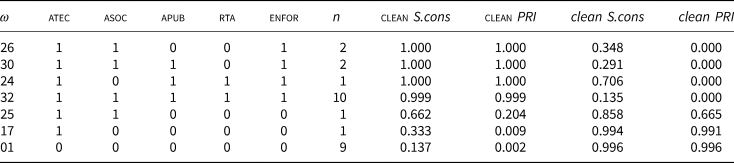
Of 32 possible realizations, seven only are observed and neatly associated with either one outcome or the other with one exception (ω ₂₅), which does not affect the analysis when run with crisp scores. Units concentrate in the two polar realizations: nine of 11 instances of the negative outcome are the best instances of ω ₁ while 10 out of 15 positive instances are best instances of ω ₃₂. Were already the model a well-specified inus machine, the concentration should be higher. Dispersion suggests alternative specifications and/or redundancies, which justifies minimizations.

The minimizations retrieve the solutions in Table 7.

Table 7. Prime implicants

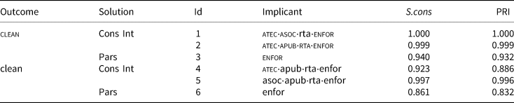
Note: Prime Implicant 1 covers 4 of the 15 instances of aut, bel; aus, can.

PI 2 covers 11 of the 15 instances of clean: fra; nzl, deu, dnk, est, fin, gbr, nld, nor, swe, usa.

No instances of clean are overdetermined.

PI 3 covers all the 15 positive instances.

PI 4 covers 2 of the 11 instances of clean: ita; prt.

PI 5 covers 10 of the 11 instances of clean: bgr, cze, esp, grc, hrv, hun, pol, rou, svn; ita.

One instance of clean is overdetermined – namely, ita.

PI 6 covers all the 11 negative instances.

The parsimonious solutions identify a single factor (the effectiveness of civil justice enforcement) that captures the whole difference between the instances of the positive and the negative outcome. The intermediate solution instead overlaps the conservative; their prime implicants use all the conditions in the model, but differently specified to special subpopulations. The settings suggest that alternative inus machines are at work in groups of instances of the realized outcome. The instances of the unrealized outcome contain one overdetermined case, in which the failure can be ascribed to one or the other of two compounds.

Letting the theoretical interpretation aside, the last open question asks which causal standing can be recognized to the information in the parsimonious and intermediate solutions.

Exploring the relationship between solution types

Fiss (Reference Fiss2011, Soda and Furnari Reference Soda and Furnari2012) dubs the conditions in the parsimonious term the ‘core’ element of the solution, while the conditions added under directional expectations are ‘peripheral’ contributors. The S.cons and PRI reported in Table 6 prove that the core provides a worse explanation when alone than in conjunction with the peripheral terms. Hence, the peripherals are relevant to the outcome, although maybe not causally so. The SCM provides the diagnostic device that clarifies the causal nature of their relationship.

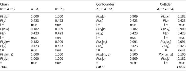
Tables 8 and 9 report the conditionalities that identify the structures of a chain, a confounder, and a collider, computed between the core condition (z), the peripheral conditions in each solution term (x ₁, x ₂), and the outcome (y) for each outcome state after turning the fuzzy scores into crisp. A fundamental causal structure is assigned to the solution term when all the identifying conditionalities are satisfied. The conditionalities are inevitably deterministic given the gauges and the single observation point. Nevertheless, in such a thin slice of the world, structures do emerge.

Table 8. Structures of the intermediate solution terms to clean

Keys: the nodes in the graphs are given the following values: y =  CLEAN; z =  ENFOR; $x_1 = {\rm TEC} \cap {\rm PUB} \cap {\rm RTA}$; $x_2 = {\rm TEC} \cap {\rm SOC} \cap \text{rta}$.

N = 26 for each node.

Table 9. Structural dependencies of the intermediate solution terms to clean

Keys: the nodes in the graphs are given the following values: y =  clean; z =  enfor; $x_1 = {\rm TEC} \cap \text{pub} \cap \text{rta}$; $x_2 = \text{soc} \cap \text{pub} \cap \text{rta}$.

N = 26 for each node.

The conditionalities of the ‘chain’ structures indicate that the core provides the mediating node between the peripheral conditions and the outcome in both the positive and the negative solutions. The conditionalities, moreover, support the claim that the core term provides neither the ‘confounding’ background common factor nor the ‘collider’ in any subpopulations – regardless of whether the peripheral terms display full set-independence [P(x ₂|x ₁) = 0.00 and P(x ₁|x ₂) = 0.00 in Table 8] or a slight dependence [P(x ₂|x ₁) = 0.091 and P(x ₁|x ₂) = 0.091 in Table 9].

These findings suggest that each of the solutions identified by the plausible minimizations renders the settings of a mechanism, and the core elements provide the ‘mediator’. Moreover, the shape suggests that the peripheral conditions do not offer alternative starting points, but equivalent backgrounds.