


I. INTRODUCTION
The interconnect media for the high-speed integrated circuits is becoming an important task for the electronic circuit designer at different levels, especially at the printed circuit board (PCB), the backplanes, the chip to chip, and the multichip designs. Many contributors have treated this subject; in [Reference Paul1] Paul gives an overview of the multi-conductor transmission lines (MTL) for electro-magnetic compatibility (EMC) applications; Nitsch et al. [Reference Nitsch, Baum and Sturm2] have investigated analytically the uniform MTL; Griffith et al. [Reference Griffith and Nakhla3] have investigated non-linear circuits using a mixed frequency and time-domain analysis; in [Reference Nakhla, Douanavis, Nakhla and Achar4], Nakhla et al. have investigated the MTL with non-linear terminations by delay extraction-based sensitivity; in [Reference Winkelstein, Pomerleau and Steer5], Winkelstein et al. have simulated a complex lossy multiport transmission lines terminated with a non-linear digital device. The interconnecting analysis would give an optimum design with a minimum transmission line effects such as the attenuation and impedance mismatching, as well for analog and digital systems; for example, the interconnect should not introduce any delay and should not modify, in particular, clock signals; also the recent developed mixed analog and digital electronic blocks require less power consumption; high-speed interconnects have been treated and simulated with a convolution-based hierarchical packaging simulator [Reference Basel, Steer and Franzon6]. Another point that needs an investigation is the cross-talk problem between the lines since the interconnects are often made of multi-conductors that are parallel to each other; this cross-talk, which is due mainly to parallel traces and backplanes, has been investigated by different contributors [Reference Paul7–Reference Maio, Canavero and Dilecce11], can be a source of error for signal transmission and will reduce the electromagnetic (EM) immunity of the system. In [Reference Deutsh12], a criterion has been developed for short, medium, and long interconnect showing the inductance effect in the signal delay and cross-talk; in [Reference Ismail, Friedman and Neves13] rules are exposed to characterize the effect of the on-chip inductance and its correlation with the line damping ratio and the signal rise time. Modeling and simulating interconnect problem has been the subject of research for few decades for many contributors leading to different methods, techniques and algorithms, such as the impulse response and convolution (IRC) method treated in [Reference Winkelstein, Pomerleau and Steer5, Reference Basel, Steer and Franzon6, Reference Djordjevic and Sarkar14, Reference Brazil15], the asymptotic waveform evaluation (AWE) method [Reference Das and Smith16–Reference Celik, Ocali, Tan and Atalar18], and the numerical inversion of Laplace transform (NILT) [Reference Chang and Kang19–Reference Honig and Hirdles23].
In the literature, different models for the interconnects have been developed; the RC tree model is not very accurate for the high-speed system, the model with the lumped circuit is used when the line is electrically short, the partial element equivalent circuit (PEEC) model and the transmission line analysis are also added when the line is electrically long especially for high-speed systems. These models need an implementation of specified algorithms for the analysis in the time domain or in the frequency domain or in both domains with linear and non-linear terminations. One main problem in the multi-conductor interconnecting networks is the excitation of the multi-conductor system by an EM wave, this problem has been widely investigated by many contributors [Reference Paul24–Reference Agrawal, Price and Gurbaxani33]. In [Reference Paul24], Paul presents three methods (spice model, time domain-to-frequency domain transformation, and finite difference time domain (FDTD) method) to solve the problem of an MTL excited by an incident EM field and to predict the voltage and current in the time domain or in the frequency domain induced at the terminations of the MTL using the transformation of the MTL equations into uncoupled model lines taking into consideration the delay lines of each mode. An hybrid method (FDTD with SPICE) has also been used for lossless transmission lines excited by a nonuniform incident electromagnetic field [47], the FDTD method is used to calculate the excitation fields of the lines leading to voltage sources, which will be incorporated easily into a SPICE model; this hybrid method has shown the possibility to solve problems with time varying or nonlinear MTL terminations. In [Reference Nitsch, Baum and Sturm2], Nitsch et al. have given an analytical solution in the frequency domain for the MTL equation based on the assumption of the commutatively between the propagation matrix and the characteristic impedance matrix taking into consideration the nature of the medium (lossy or lossless, uniform, and isotropic).
In [Reference Bernardi, Cicchetti and Pirone34], Bernardi et al. have studied the transient voltage and current induced by an external EM along a dispersive line and a no dispersive line, and also has treated the coupling between an incident field arbitrarily varying in time and a microstrip line interconnecting active or passive component by considering the per unit length surface charge on the strip and the electric field in the substrate. In [Reference Das and Smith35], the time-domain simulation of the AWE was presented and extended to the application of a lossless interconnect networks excited by an incident uniform plane wave. In [Reference Rachidi36], Rachidi has given a brief review of the different formulation of the EM wave coupling to transmission lines and presents a new formulation for the sources terms expressed only by the magnetic fields' components making it easy to calculate the EM coupling by knowing only the magnetic fields' components. In [Reference Shinh, Nakhla, Achar, Nakhla, Dounavis and Erdin37], a transient analysis is given in the case of lossy MTL excited by an incident field and has proposed an equivalent distributed sources due to the electromagnetic interferences (EMI) allowing fast computation time.
The purpose of this paper is to study the EM field coupling to an MTL system using the NILT method and to find the near-end and far-end cross-talk for the two types of microwave (MW) structures; in Section I, theoretical formulations of the problem are presented; in Section III, the numerical simulation procedure and results are given, and in Section IV, conclusion and discussions concerning the subject are deduced.
II. THEORETICAL FORMULATIONS OF AN MTL SYSTEM EXCITED BY AN EM WAVE
The MTL system is the best-fitted modeling configuration for the MW interconnects and the interaction of EM waves with the MTL system is usually analyzed in terms of voltage- and current-induced sources distributed along the lines.
The distributed linear- and frequency-dependent circuit elements have been simulated in the transient analysis by different methods such as the IRC, the interpolation method, the AWE, and the NILT; the IRC method has been used in [Reference Djordjevic and Sarkar14] to model distributed multi-conductor MW circuits; also the IRC method has been improved by other contributors, in [Reference Winkelstein, Pomerleau and Steer5] low-pass filtering has been introduced to minimize the aliasing error in the inverse fast Fourier transform, the non-linear concept [Reference Basel, Steer and Franzon6] has been included in the study of some circuits, the insertion of time delay in the analysis has given results with a minimum distortion [Reference Brazil15], also the results are optimized by using the [S] parameters [Reference Schutt-aina and Mittra38]; the AWE method is a well-fitted model for the digital system [Reference Chiprout and Nakhla17, Reference Celik, Ocali, Tan and Atalar18] and it is a reduction model technique based on the optimization of a rational polynomial transfer function by minimizing the distortion [Reference Chan39] based on the Pade approximation leading to a stability problem as any other approximations. Unlike methods using Fast Fourier Transform (FFT), the NILT method does not have the causality problem for double-sided Laplace transforms and an other advantage is that the aliasing problem will not occur in the NILT method, since the considered function is not necessarily periodic and the inverse Laplace transform can be calculated for periodic and for non-periodic functions; the main difficulties of using the NILT method are the well-fitted approximation of the series and the non-linear interactions, in [Reference Griffith and Nakhla3] a description of the NILT method is given by presenting its limitations and advantages.
In this paper, the effect of the EM coupling is treated and it is based on the superposition effect of each distributed voltage current sources using the NILT numerical method.
A) The coupled MTL equations
The commonly used equations to analyze the EM coupling effect into a MTL system with N + 1 conductors, as shown in Fig. 1, are developed in many references as a coupled system of partial differential equation in function of the voltage and current lines represented by vectors of dimension n, respectively, [v(y, t)] and [i(y, t)]
with [L], [C], [R], and [G] are the (N × N) matrices representing, respectively, the per unit length inductances, capacitances, resistances, and conductances.

Fig. 1. MTL system.
The effect of the incident EM field into (N + 1) conductors is given in terms of forcing functions as a distributed source voltage vector [v ds(y, t)] and a distributed source current vector [i ds(y, t)] with dimension n, and are defined in terms of the incident EM wave:
[E T(y, t)] and [B N(y, t)] are, respectively, the vector of the tangential components of the incident electric field and the vector of the normal components of the incident magnetic induction to the surface of the different conductors; they are defined by the following expressions:
With c j defined as the contour from the reference conductor (ground plane) to the jth conductor lying in the transverse (z, x) plane.
In the frequency domain and assuming the quasi-TEM mode, the state variable form of an MTL system excited by an incident field is given by
With the matrices [Z] = [R] + s[L] and [Y] = [G] + s[C];
[V(y, s)] and [I(y, s)] are, respectively, the Laplace transform of the vector voltage [v(y, t)] and the vector current [i(y, t)] at a point y and the conductors are parallel to the y-axis; s represents the complex variable of the Laplace transform; [V ds (y, s)] and [I ds (y, s)] are, respectively, the Laplace transform of the forcing voltage [v ds(y, t)] and forcing current [i ds(y, t)].
Using Maxwell–Faraday's law, the forcing voltage and current distributed sources [V ds(y, s)], [I ds(y, s)] can be also expressed only by the transverse and the longitudinal electric fields.
Let the ground plane at z = 0 and the jth trace is located at the height z = z j, the equivalent distributed sources for the jth transmission line (jth trace and ground) due to the EMI can be rewritten in terms of incident electric field components:
where E yin, E zin are, respectively, the longitudinal and the transverse component of the electric incident field; Y j = G jj + sC jj is the admittance per unit length of the jth transmission line. Equation (4) can be written in a matrix form as
With ![]() and
and ![]()
The solution for the voltage and current of the above equation (6) at any point y is given in [Reference Paul40] as
where Φ(y) = e[Q]y and
The resolution of the first term of the above equation, which is considered as a delay part due mainly to the presence of the frequency-dependent components (L, C), has been treated by Shinh et al. [Reference Shinh, Nakhla, Achar, Nakhla, Dounavis and Erdin37] as an association of lossless and lossy transmission lines.
The last term of the above equation represents a spatial convolution of the distributed sources (V ds, I ds) with an exponential term due to the MTL configuration, its numerical resolution is easy to evaluate especially in the time domain because the distributed voltage and current sources are a function of a matrix exponential. In fact, this term depends on the distributed source location, therefore, the complexity form of the time-domain expression has been simplified in [Reference Bridges and Shafa30], in which the EM coupling effect of a plane wave on an MTL has been analyzed and has proposed an equivalent model that is constituted principally by:
– A near-end equivalent distributed voltage [V sn] and current [I sn] sources due to the EMI.
– An unexcited MTL.
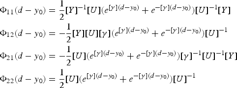
– A far-end equivalent distributed voltage [V sf] and current [I sf] sources due to the EMI. Therefore, the given solution for equation (7) is approximated by a line length d:
(9)
With ![]() and
and ![]()
This model can be efficient for relatively low-frequency EM coupling, but for MW and millimeter circuits is not possible to consider the EM coupling as located sources at the terminals; therefore, in the next section, in order to evaluate efficiently the transient analysis, we propose a linearized NILT taking into consideration the different distributed forcing voltages and currents. The considered MTL system is constituted by N transmission lines; the jth conductor is located at the height z j from the ground plane and has a length d j and having the following characteristics:
– propagation constant
If the incident excitation EM field does not exist [T ds] = [0] then the general solution is given in [Reference Paul40] by a chain parameter matrix:
With Φij are N × N matrices:
where [U] is an N × N non-singular matrix introduced by the similarity transformation which makes a change of variable; V(y, s) = [U V][V m(y, s)] and I(y, s) = [U I][I m(y, s)] with [V m(y, s)] and [I m(y, s)] are the mode voltages and currents which are solutions of the eigenvalue problems:
the current and the voltage line at any point y can be written, respectively, as I(y, s) = ∑ I me ±γmy, V(y, s) = ∑ V me ±γmy taking into consideration the progressive and regressive waves along the lines.
[U] = [U I] if we choose to decouple the second-order MTL differential equation in current and [U] = [U V] if we choose to decouple the second-order MTL differential equation in voltage. The propagation matrix [γ] is a diagonal matrix of the eigenvalues of [U]−1[Y][Z][U].
– characteristic impedance
From the above analysis it is given, in [Reference Paul40], that the characteristic impedance matrix as
– [Z 0] = [Y]−1[U][γ][U]−1 in terms of admittance inverse matrix [Y]−1or [Z 0] = [Z][U][γ]−1[U]−1 in terms of impedance matrix.
– Time delay
This parameter will be present mainly due to the frequency-dependent components, therefore the MTL second-order differential equations in the time domain can be written as
If we suppose that the jth line voltage is written as v j(y, t) = g(y − v 0jt) with v 0j the propagating wave speed in the line, then we can write that ![]() and λ j are the eigenvalues of the matrix [L][C], j = 1, 2, … , N; and the time delay can be assumed as T Dj = (d j/v 0j).
and λ j are the eigenvalues of the matrix [L][C], j = 1, 2, … , N; and the time delay can be assumed as T Dj = (d j/v 0j).
B) NILT procedure method
In order to have an accurate estimation of the transmission line effects related to the interconnects, especially when the line length is similar to the wavelength of the considered signal, a linearized computational method is presented and implemented in MATLAB environment based on the NILT that is considered as an efficient time-domain numerical method for the interconnects modeling, and it has been widely used for the different models (RC tree, lumped circuit, PEEC with or without frequency-dependent parameters, and lossy-coupled MTL). The NILT method, which is developed in [Reference Hosono20–Reference Honig and Hirdles23], has been chosen because the calculation of the exponential matrix e −Q(s)d in the convolution expression is not necessary for the prediction of the transient analysis and the numerical calculation of the spatial convolution [T sd(y, s)] as expressed in (8) is simple to discretize by using the expansion of Φ(y). It is well known that the Laplace transform F(s) of the real-valued function f(t) and its inverse Laplace transform:
where σ is such that the contour of integration is to the right-hand side of any singularities of F(s). NILT is developed to give an approximation of e st in order to determine the complex integral. This method has enormous advantages as a simple algorithm for implementation, relatively accurate computation with controllable errors, and can be applied in many applications. In order to find the original signal f(t) from the Laplace transform F(s) using the well-known NILT method, it is necessary to make some assumptions and mathematical conditions for f(t) and F(s), which are given in Table 1.
Table 1. Conditions for the f(t) and F(s) used in the NILT method.

There are mainly three different methods to calculate the integral to determine f(t):
– The integration algorithm requires a long time for running program, since the upper limit of the integral is increased for better accuracy.
– The Zakian algorithm that is easy to implement, based on a sum of weighted evaluation of F(s), and it is not accurate for under-damped systems.
– The FFT algorithm in which the F(s) is evaluated at a sequence of frequency values for a specific maximum value of time and a well-chosen value of σ for a relative error E.
The used algorithm in this work is based on Fourier series expansion and the continued fractional approaches.
Equation (15) can be expressed also by the following equation [Reference Paul40]:
Using the trapezoidal rule with a step size of π/T, and the discretized approximation is obtained for 0 < t < 2T:
![f\lpar t\rpar = \displaystyle{1 \over T}e^{\sigma t} \left[{\displaystyle{{F\lpar \sigma \rpar } \over 2} + \sum\limits_{n=1}^\infty {{\mathop{\rm Re}\nolimits} \Bigg [F\left({\sigma + j\displaystyle{{n\pi } \over T}} \right)} e^{j\lpar n\pi t/T\rpar } } \Bigg] \right]+ E](https://static.cambridge.org/binary/version/id/urn:cambridge.org:id:binary:20151130141448579-0889:S1759078712000153_eqn17.gif?pub-status=live)
Numerically, the infinite series must be truncated after a sufficient number of terms, and this truncation will be a source of error; E presents the discretization error and E is very small when the series terms are large, then we have an approximation of f(t):
![f\lpar t\rpar \approx \displaystyle{1 \over T}e^{\sigma t} \left[{\displaystyle{{F\lpar \sigma \rpar } \over 2} + \sum\limits_{n=1}^\infty {{\mathop{\rm Re}\nolimits} \Bigg [ F\left({\sigma + j\displaystyle{{n\pi } \over T}} \right)} e^{j\lpar n\pi t/T\rpar } } \Bigg ]\right]](https://static.cambridge.org/binary/version/id/urn:cambridge.org:id:binary:20151130141448579-0889:S1759078712000153_eqn18.gif?pub-status=live)
The main problem in the evaluation of the infinite series is that it converges very slowly and to accelerate the evaluation of the series different methods have been developed such as the quotient difference method that has been developed by Rutishauser [Reference Rutishauser41] and was used to calculate the coefficients of the continued fraction to a given power series [Reference Henrici42].
Then it is possible to evaluate rapidly the infinite series in equation (18) using the rational approximation in the form of a continued fraction.
Let us consider a power series p(z) and c(z), and the continued fraction associated with p(z)
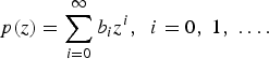
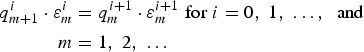
For the given coefficients bi of the power series p(z), we initialize ɛ0i = 0 and q 1i = (b i+1/b i)
A system of recursive formulation is given
the corresponding diagram of q mi and ɛmi are presented in Fig. 2 and the corresponding coefficients k m are expressed by the following equations:

Fig. 2. Diagram of ɛmi and q mi.
By setting b 0 = (F(σ)/2), b n = F(σ + j(nπ/T)), and z = e j(πt/T), we can apply the quotient difference algorithm to evaluate the NILT f(t) ≈ (1/T)eσtp(z); for the truncation of order M, the continued fraction c(z, M) corresponding to the power series p(z) is
And the successive convergent c(z, 1), c(z, 2), … of the continued fraction are obtained by using the recurrence relations given in [Reference Henrici42]:
With m = 1, 2, 3, …; α −1 = 0, β −1 = 1, α 0 = k 0, and β 0 = 1. Then c(z, M) = (α M/β M) and f(t) is approximated as f(t) ≈ (1/T)e σtRe(c(z, M)).
By considering the diagonal-wise operations combined with the recursive relations (25), we can determine k m, α m, and β m as indicated in Table 2 for the first three diagonals.
Table 2. Determination of the different coefficients for the ith diagonal.

After the (M − 1)th diagonal parameters, the elements of the Mth diagonal are calculated and we obtain f(t) with a truncation error E M:
It is not an easy task to evaluate the truncation error of the continued fraction and for a relatively error E; Honig and Hirdles [Reference Honig and Hirdles23] have shown that σ should be chosen to be σ = γ − (log E/2T) with the number γ ≈ max(Re(pole of F(s)).
Table 2 summarizes how to determine the different coefficients for the ith diagonal. For each rhombus centered in a q-column, the sums of the upper elements to the right are equal to the sum of the two lower elements to the left (equation (21)) and for each rhombus centered in an ɛ-column; the corresponding products are equal (equation (22)).
C) Time-delay effect on the MTL system
The well-known theory in the frequency domain of a coupled MTL, leads to the following expressions of the vector voltage [V(y, s)] and the vector current [I(y, s)] by including the concept of mode propagation; for the jth conductor with the propagating mode, its voltage and current are given by:
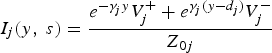
Where V j+, V j−, γj, and Z 0j are, respectively, the forward-propagating term, the backward-propagating term, the mode propagation constant, and the mode impedance characteristic for the jth transmission line. It is to be noted that the boundary conditions of telegraph equations are time-dependent and the values of the equivalent circuit elements are dependent on the terminal voltages.
Using the characteristic formulation [Reference Branin43–Reference Chang45], and by considering the near end voltage vector [V(0, s)] = [V n(s)] and the far-end voltage [V(d, s)] = [V f(s)], and similarly for the near-end current [I(0, s)] = [I n(s)] and for the far-end current [I(d, s)] = [I f(s)], an MTL system with n + 1 conductors can be considered then as a 2N port network, as shown in Fig. 3, having 2N voltage sources and 2N characteristic impedances and the time domain results of the simulation are given by using the characteristic impedances of the considered equivalent network and by evaluating the convolution of e−γjd j with the different voltages [V f], [V n], [E 1], and [E 2].

Fig. 3. The equivalent 2N port network for the MTL system.
With the vectors [E n] and [E f] of dimension N represent the waveform generators:
The transient analysis can be achieved by using the equivalent distributed element circuits for the characteristic impedance and by determining the convolution integrals for E nj and E fj.
Once the considered interconnects are modelled by the equivalent network, two steps have to be achieved with accuracy:
– The evaluation of the characteristic impedance.
– The evaluation of the two generators.
The characteristic impedance evaluation is treated by different methods mainly the Pade approximation and non-linear optimization techniques, and the result leads to an RLCG equivalent circuit. Concerning the evaluation of the generators in the time domain, there are also different methods, mainly the use of NILT.
Authors of articles published in the journal assign copyright to Cambridge University Press and the European Microwave Association (with certain rights reserved), and a copyright assignment form must be completed on acceptance of your paper.
III. SIMULATION PROCEDURE AND RESULTS WITH AN EM PLANE WAVE EXCITATION
The NILT method is implemented first to analyze and then to determine at any point of the MTL system the current and voltage of the different transmission lines in the time domain; in order to analyze the effect of the EM incident waves to the MTL system that leads to the equivalent transmission lines having distributed forcing current and voltage sources (Fig. 4), we use a linearized NILT method based on the Norton–Thevenin transformation and the superposition concept.

Fig. 4. The equivalent circuit for a transmission line excited by an incident EM field.
For that, if we assume that there is M distributed current sources and M distributed voltage sources, and each current and voltage source are placed in an elementary length Δy of the transmission line; the effect of each current and voltage source is calculated using the NILT method by eliminating the other distributed sources and by evaluating the equivalent termination impedance Z j (Fig. 5).

Fig. 5. Norton–Thevenin transformation of a transmission line excited by a single source.
The total effect of the EM coupling is obtained after M simulation of the NILT method.
The incident electric field plane wave is expressed in [Reference Das and Smith16] by

With β x = −β sin θ cos φ, β y = −β sin θ sin φ, β z = −β cos θ and ![]() .
.
The forcing distributed current and voltage source for the ith transmission line can be expressed in terms of the Laplace variables [Reference Paul46] by

At first, the results of the proposed method are used for a single transmission line, and the induced voltage and current at the near and far ends are presented in Fig. 6 for an oblique incidence of θ = π/4 and is compared with the results given in the literature, showing similar results with an approximate error due to the evaluation of the effective dielectric constant and due to the truncation error E M to evaluate the function f(t) corresponding to the transient voltage and current. We can note that incidence angle has an effect on the calculated distributed voltage and current sources; in the case of θ = π/4, the electric field coupling is most important than the magnetic field coupling.

Fig. 6. Induced transient voltage (a) and current (b) along a single transmission line at the near and far ends.
In order to make MW structures with less EM field coupling, we make simulations for two different planar structures A and B, as shown in Fig. 7, and are chosen as the MTL system with 3 + 1 conductors and numerical comparison of the transient EM field coupling at the ends of the traces using the proposed algorithm based on the NILT method.

Fig. 7. Cross-sectional view of the two structures.
On the one hand, the homogeneous structure A gives relatively important transient voltages due to the EM coupling at the near and far ends of the three traces as shown in Figs 8(a) and 8(b), respectively.

Fig. 8. The transient-induced voltages for the three traces at the near (a) and far (b) ends for the homogeneous structure A.
On the other hand, the numerical study of the non-homogeneous structure B gives different aspects as shown in Figs. 9(a) and 9(b), which represent, respectively, the transient voltage due to the EM coupling at the near- and far-end voltages for the second trace in two cases (ɛ r1 < ɛ r2 and ɛ r1 > ɛ r2). The simulation results show that a well-designed multilayered substrate (ɛ r1 < ɛ r2) gives a minimum transient EM coupling due to an external EM field; and it shows also that, for θ = π/4, the electric coupling is mainly important than the magnetic coupling.

Fig. 9. The transient-induced voltage for the second trace at the near (a) and far (b) ends for the non-homogeneous structure B for the two considered cases.
IV. CONCLUSION
The NILT method has been used in this paper to simulate and estimate the transient effect of an EM incident field illuminating a multiconductor transmission lines; for this purpose, we proceed by simplifying the excited MTL with M distributed current sources and voltage sources by M equivalent circuits as shown in Fig. 5 using the Northon–Thevenin transformation; the use of the superposition concept of the different simulation from the NILT method leads to the final response for the line current and line voltage in the time domain.
The proposed computing model for EM field coupling to the MTL system is based on the NILT method, which is a fast numerical method implemented in the MATLAB environment and it has shown sufficient results since it takes into consideration all the distributed current and voltage sources along the different lines by including the different physical concepts such as the linearity of the equivalent circuit, the time delay of the different lines, the impedance matching and the incidence angle. The results of the simulation are given for two MW structures (homogeneous and non-homogeneous). The multi-dielectric non-homogeneous structure leads to two configurations (ɛ r1 < ɛ r2 and ɛ r1 > ɛ r2) and in the case when ɛ r1 < ɛ r2 the simulation results show that the EM field coupling can be minimized by a well-designed MTL system with multi-dielectric substrates comparatively to a single dielectric substrate.
 Adnen Rajhi received an M.Sc and a Ph.D. in electrical communication from Tohoku University in Japan, respectively, in 1990 and 1994. Since 1998, he has been with the Department of Electrical Engineering at the University of Cartage; his research interests include electrical and electronic systems and EMC problems.
 Said Ghnimi received a degree in electronics engineering in 2004 and M.Sc. degree in electronics device from El-Manar University – Sciences' Faculty of Tunis, Tunisia, in 2006. He is currently working toward his Ph.D. degree in electrical engineering at the Sciences' Faculty of Tunis. His research interests include Electro-Magnetic Compatibility (EMC), telecommunication systems, and microwave-integrated circuits.
 Ali Gharsallah received the degree in radio-electrical engineering from the Engineering School of Telecommunication of Tunisia in 1986 and the Ph.D. degree in 1994 from the National School of Engineering of Tunisia. Since 1991, he has been with the Department of Physics at the Sciences' Faculty of Tunis. His current research interests include antennas, array signal processing, multilayered structures, and microwave-integrated circuits.


