


Introduction
Effectively detecting the enemy early warning radar is vital. Satellite system can realize the beyond line-of-sight (b-LoS) detection. However, it has security problems and may be interrupted by the hostile jamming. Furthermore, satellite system generally uses the image recognition technology to search its targets, which is relatively powerless to detect the radiation sources in disguise or in blind areas [Reference Yang, Xu and Li1]. Troposcatter is a promising candidate for the b-LoS propagation. Electromagnetic (EM) wave of hostile radar propagated by troposcatter can be utilized for the b-LoS detection [Reference Wang, Wang, Wang, Cheng and Zhang2–Reference Li, Chen and Liu5].
To improve the maneuverability of passive troposcatter detection system, [Reference Wang, Wang, Wang, Cheng and Zhang2] has designed a receiving antenna mode based on the signal group delay. This mechanism can conveniently and inexpensively locate targets on the basis of only single station rather than multi-stations. High propagation loss is one of the main characteristics of troposcatter. In [Reference Luini, Capsoni, Riva and Emiliani3], a comprehensive method for predicting propagation loss has been presented. Troposcatter is also marred by the multipath fading, [Reference Wang, Wang, Cheng and Chen4] has studied troposcatter transfer function, and proposed a fading correlation model to handle the signal received by the array antenna.
Although the passive troposcatter detection system has been well studied, there is no analytical study on the operating range, which is also an important factor in radar system. Estimating propagation loss is a key step to predict the operating range; the statistical propagation loss model is firstly analyzed in this paper. According to the existing researches [Reference Wang, Wang, Cheng and Chen4, Reference Li, Chen and Liu5], time-varying meteorological parameters have obvious effect on tropospheric refractivity, which dominates the performance of troposcatter links. To estimate the dynamic operating range, the specific relationship between propagation loss and refractivity is presented. Furthermore, Hopfield model is introduced to precisely describe the refractivity at any altitude. Finally, we predict the operating range according to above discussion. The chief innovations of this paper are mainly focused on twofold. On the one hand, we innovatively predict the operating range of passive troposcatter detection system. On the other hand, operating range is predicted through dynamic loss model, instead of the conventional model.
In this paper, we study the operating range of passive troposcatter detection system; the characteristics of troposcatter including propagation loss and refractivity are also presented. The rest of this paper is organized as follows. Way to predict the operating range as well as different propagation loss models are given in “Operating range of passive detection system” section. In “Example analysis” section, some examples are displayed. “Conclusions” section draws the conclusion.
Operating range of passive detection system
Figure 1 shows the principle of passive troposcatter detection system. EM wave of enemy radar propagated by troposcatter can be detected by our system. Current signal detection algorithms mainly focus on matched filter detection, cyclostationary feature detection, and energy detection (ED) [Reference Li, Chen and Liu5]. Different from cooperative occasions, passive system probably lacks priori knowledge on the targets [Reference Conti, Berizzi, Martorella, Dalle Mese, Peteri and Capria6]. ED which has simpler implementation and less requirement of priori knowledge is a preferred candidate for passive troposcatter detection system. Energy level of the received signal dominates the consequence of ED. Namely, key to predict the operating range lies in estimating the received power, which can be given as
 $$P_r = P_t-L_\Sigma, $$
where P t denotes the transmitting power of enemy radar, P r represents the power received by detection system, L Σ is the propagation loss, which has obvious relationship with the distance between detection system and enemy radar. Only P r ≥ S, the detection system can work normally, here S is the receiver sensitivity. Hence we can estimate the operating range through the equation: P r = S. Precisely calculating L Σ is vital to predict the operating range.
Fig. 1. Passive troposcatter detection system.
Statistic propagation loss model
Several statistic models for estimating the propagation loss have been proposed. Zhang model has been internationally accepted [Reference Zhang7]. The main propagation loss of a troposcatter channel can be given as
 $$L = F + 30{\rm 1g}\;f + 30{\rm 1g}\Theta _0 + 10{\rm 1g}\;d + 20{\rm 1g}(5 + \gamma H) + 4.34\gamma h_0 + L_c,$$
where Θ0 refers to the least scatter angle (mrad), which can be calculated as Θ0 = θ t + θ r + 1000d/a e, here, a e is the median effective earth radius. θ t, θ r are the transmitter and receiver horizon angle, respectively. F denotes the meteorological parameter (dB), γ represents the atmospheric structure coefficient (km−1), f denotes the frequency (MHz), d refers to the path length between the receiving and transmitting antennas (km). H denotes the height between the lowest scattering point and the connection between receiving and transmitting antennas (km), which can be expressed as H = 10−3Θ0d/4. h 0 represents the height between the lowest scattering point and ground (km), which can be calculated as  $h_0 = 10^{-6}\Theta _0^2 a_e/8$.
The aperture-to-medium coupling loss of an antenna [Reference Li, Wu, Lin, Zhang and Zhao8] can be generally expressed as
 $$L_c = 0.07 \times e^{0.055 \times (G_t + G_r)},$$
where G t, G r stand for the plane wave gains of TX/RX antennas, respectively. Both of them can be given as
 $$G_{t,r} = 101{\rm g}[4.5 \times (D/\lambda )^2],$$
where D denotes the antenna diameter. Therefore, L Σ can be finally calculated as
 $$L_\Sigma = L-(G_T + G_R).$$
Although Zhang model can effectively estimate the propagation loss, the time resolution and spatial resolution are relatively poor.
Dynamic propagation loss model
The received power of a troposcatter link can be defined as [Reference Li, Chen and Liu5, Reference Dinc and Akan9]
 $$P_r = P_t\int_V {\displaystyle{{\lambda ^2G_TG_R\sigma _v\rho} \over {{(4\pi )}^3{(r_1r_2)}^2}}} dV,$$
where λ denotes the wavelength, r 1 (r 2) represents the distance between the scatter point to TX(RX), σ v is the scattering cross-section. ρ denotes the aperture-to-medium coupling factor, which can be expressed as L c = −101gρ. V refers to the common volume, which can be approximated as
 $$V = 1.206\displaystyle{{r_1^2 r_2^2 \delta _t\delta _r\phi _t\phi _r} \over {\sqrt {r_1^2 \phi _t^2 + r_2^2 \phi _r^2 \sin \Theta}}}, $$
where Θ is the scattering angle. δ t,r denotes the half power beamwidth of transmitting and receiving antennas in the vertical direction. ϕ t,r represents the half power beamwidth in the horizontal direction. They can be modeled as
 $$\delta _{t,r}(\phi _{t,r}) = (70{\rm ^\circ} \sim 75{\rm ^\circ} ) \times \lambda /D.$$
According to Kolmogorov theory, σ v can be expressed as
 $$\sigma _v = 2\pi k^4 = \sin ^2\chi ^\Phi (K_s)$$
where k = 2π/λ represents the wavenumber. χ = π/2 for the horizontally polarized EM wave, χ = π/2 + Θ for the vertically polarized EM wave. Φ(k s) can be calculated as
 $$\Phi (k_s) = 0.0033k_s^{-m} C_n^2, $$
where m = (11/3,5). Other parameters can be given as
 $$\left\{ \matrix{k_s = 2k\sin (\Theta /2) \hfill \cr C_n^2 (\Lambda_0,M) = 2.8\Lambda_0^{4/3} M^2 \hfill} \right.,$$
where Λ0 represents the outer scale of atmospheric turbulence, which can be written as
 $$\Lambda _0(h) = \left\{ \matrix{0.4h,\quad 0 \le h \le 25\,{\rm m} \hfill \cr 2\sqrt h, \quad 25 \le h \le 1000\,{\rm m} \hfill \cr 63.24,\quad h \ge 1000\,{\rm m} \hfill} \right..$$
In equation (11), M stands for the vertical gradient of tropospheric refractive index. According to the tropospheric theory, n = 1 + 10−6N, here, n, N refer to the tropospheric refractive index and refractivity, respectively. N = N dry + N wet [Reference Gong, Yan and Wang10], here, N dry, N wet refer to the dry and wet terms of refractivity, respectively. Both of them can be expressed as [Reference Grabner, Pechac and Valtr11]
 $$\left\{ \matrix{N_{dry} = 77.6P/T \hfill \cr N_{wet} = 373256e/T^2 \hfill} \right.,$$
where P denotes the atmospheric pressure in hPa, e represents the water vapor pressure in hPa, and T is the absolute temperature in K. Consequently, M can be deduced as
 $$\displaystyle{{dn} \over {dh}} = \displaystyle{{77.6} \over {{10}^6}}\left[ {\displaystyle{1 \over T}\displaystyle{{dp} \over {dh}}-\left( {\displaystyle{\,p \over {T^2}} + \displaystyle{{9620e} \over {T^3}}} \right)\displaystyle{{dT} \over {dh}} + \displaystyle{{4810} \over {T^2}}\displaystyle{{de} \over {dh}}} \right].$$
As displayed in equation (14), estimating M through this way depends on precisely vertical gradient of meteorological parameters. ITU-R P. 835-5 gives a troposphere model based on latitude areas (low-latitude, mid-latitude, and high-latitude) and seasons (summer and winter) [12]. For example, model of mid-latitude area in summer can be expressed as
 $$\left\{ \matrix{T_{sum}(h) = 294.9838-5.2159h-0.07109h^2 \hfill \cr P_{sum}(h) = 1012.8186-111.5569h + 3.864h^2 \hfill \cr \rho_{sum}(h) = 14.3542\exp [-0.4174h-0.0229h^2 + 0.001007h^3] \hfill \cr e(h) = \rho (h)T(h)/216.7 \hfill} \right.,$$
where h denotes the altitude. Parameter M at any h can be estimated according to equation (14) and (15). However, both time resolution and spatial resolution are relatively poor, we cannot get the real-time refractivity through this model. Meteorological parameters of three observations in mid-latitude region are selected to display the change law of tropospheric refractivity. Table 1 displays the concrete information of these observations.
Table 1. Information of three observations

Figures 2(a) and 2(b) depict the refractivity of a whole year and first 3 days of a year, respectively. From Fig. 2, we can get that the refractivity of all observations is different and apparently changes with time. Namely, ITU model cannot describe the tropospheric refractivity in more detail. The refractivity model with better performance is in urgent need.
Fig. 2. Refractivity of three observations. (a) Refractivity of a year, (a) refractivity of 3 days.
Hopfield model [Reference Hopfield13] is widely used in satellite system, it can describe N(h) as
 $$N_i(h) = \displaystyle{{N_{i0}} \over {H_i^4}} (H_i-h)^4\quad i = {\rm dry,wet,}$$
where H dry, H wet denote the equivalent height for hydrostatic and wet refractivity, respectively. They can be given as
 $$\left\{ \matrix{H_{dry} = 40136 + 148.72(T_0-273.16){\rm m} \hfill \cr H_{wet} = 11\,000\,{\rm m} \hfill} \right..$$
The vertical gradient of tropospheric refractive index can be further deduced as
 $$\displaystyle{{\partial n(h)} \over {\partial h}} = \displaystyle{{-4} \over {{10}^6}}\left[ {\displaystyle{{N_{dry0}} \over {H_{dry}^4}} {(H_{dry}-h)}^3 + \displaystyle{{N_{wet0}} \over {H_{wet}^4}} {(H_{wet}-h)}^3} \right].$$
According to equation (18), Hopfield model can directly estimate M through meteorological parameters of surface. It does not depend on vertical gradient of meteorological parameters. Ref. Reference Liu, Chen, Li and Liu14 employs several observations locating in different zones to show the performance of Hopfield model and ITU model. The consequences indicate that the former has obvious advantages. Table 2 shows bias of annual mean loss estimated by Zhang method and the time-varying method. Here, 1 stands for equator, 2 continental subtropical, 3 marine subtropical, 4 desert, 5 continental temperate, 6 sea, 7 marine temperate. Analogous consequences of different regions indicate that the dynamic method is logical. Detail information of climate zones is same as Fig. 1. Analogous consequences of two methods indicate that the latter method can also effectively estimate the propagation loss.
Table 2. Bias of propagation loss estimated by two models (dB)

Rain attenuation model
Precipitation will affect the performance of many wireless links. Because the frequency of early warning radar always ranges in microwave bandwidth, rain has relatively obvious effect on the troposcatter link [Reference Abdulrahman, bin abdurahman, kamal bin Abdulrahim and Kesavan15].
Figure 3 shows the troposcatter link under rain weather. Only the EM wave passing through rain cell will suffer from the additional attenuation. Without considering the rain scatter, the attenuation rate can be expressed as
 $$\gamma _R = k\cdot R^\gamma \;{\rm dB}/{\rm km,}$$
where R denotes the rainfall rate (mm/h), k, γ are the empirical coefficients, the value of them can be found in ITU-R P.676-11 [16]. Figure 4 displays the γ R changing with frequency. Rain attenuation becomes more obvious with the frequency increasing. Rain attenuation also depends on the length of wave passing in rain cell, [Reference Dinc and Akan17] introduces a reasonable method.

Fig. 3. Troposcatter communication in rain cell.

Fig. 4. Attenuation rate in rain cell.
As stated above, the received power follows
 $$S = P_t-L_\Sigma -L_R,$$
where L R denotes the rain attenuation. Operating range determines the propagation loss, it can be further deduced through equation (20).
Example analysis
In this section, some examples are analyzed. Figure 5(a) depicts annual mean range changing with θ r under channel parameters: f = 2 GHz, D T = 10 m, D R = 5 m, θ t = 1°, P t = 25 kW, S = −90 dBm. R = 30 mm/h, path length of EM wave passing through rain cell is 50 km. θ r = 0.5°, the other parameters are same as above, operating range changing with P t and f is displayed in Figs 5(b) and 5(c), respectively.
Fig. 5. Mean operating range of passive troposcatter detection system. (a) Operating range changing with θ r; (b) operating range changing with P t; (c) operating range changing with f.
From Fig. 5, the passive system can realize b-LoS detection. System located in the relatively moist area has further operating range. This phenomenon indicates that the moist atmosphere is beneficial for EM wave propagation. The undesirable effect caused by rain will be apparent with the frequency increasing. Parameters are same as above, real-time operating range during a year is shown in Fig. 6. The operating range during the whole year is different, and the maximum operating range appears in summer. Both Figs 5 and 6 demonstrate the feasibility of prediction on operating range of passive troposcatter detection system.
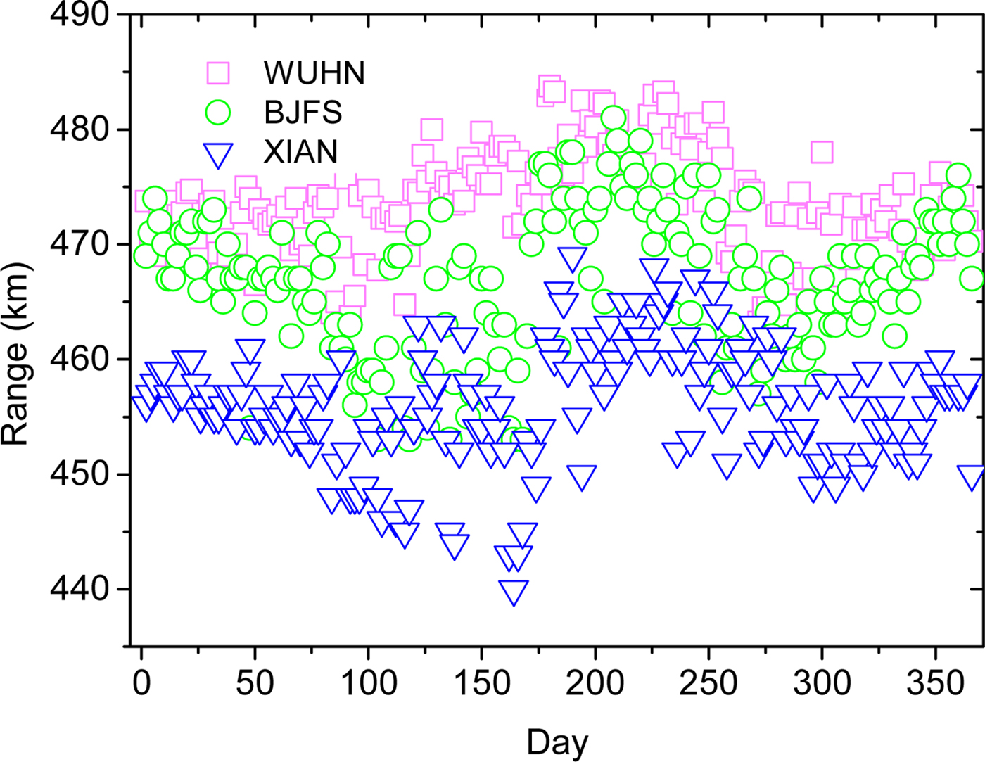
Fig. 6. Real-time operating range during a year.
Conclusions
In this paper, we predict the operating range of passive troposcatter detection system on the basis of propagation loss model. In addition, the dynamic propagation loss model improved by Hopfield model is proposed. According to our results, passive troposcatter detection system can realize b-LoS detection. As well, prediction on operating range is feasible, moist atmosphere is beneficial for passive troposcatter detection system.
Acknowledgements
We are grateful to Global Geodetic Observing System (GGOS) for providing the related meteorological data. We also gratefully acknowledge anonymous reviewers who read and make insightful and constructive suggestions. The authors declare that there is no conflict of interests regarding the publication of this paper. This work was supported by the National Natural Science Foundation of China under grand No. 61671468 and 61701525.
 Zan Liu received the B.S. and M.S. degrees in 2013 and 2015, respectively, from Air Force Engineering University, Xi'an. He is currently working toward the Ph.D. degree in the Air and Missile Defense College. His research interests include information theory and passive radar system.
 Xihong Chen received the M.S. degree in Communication Engineering from Xidian University, Xi'an, in 1992 and the Ph.D. degree from Missile College of Air Force Engineering University in 2010. He is currently a professor with Air and Missile Defense College, AFEU, Xi'an. His research interests include information theory, information security, and signal processing.


